Ultimate precision of adaptive noise estimation

Abstract

We consider the estimation of noise parameters in a quantum channel, assuming the most general strategy allowed by quantum mechanics. This is based on the exploitation of unlimited entanglement and arbitrary quantum operations, so that the channel inputs may be interactively updated. In this general scenario we draw a novel connection between quantum metrology and teleportation. In fact, for any teleportation-covariant channel (e.g., Pauli, erasure, or Gaussian channel), we find  that adaptive noise estimation cannot beat the standard quantum limit, with the quantum Fisher information being determined by the channel’s Choi matrix. As an example, we establish the ultimate precision for estimating excess noise in a thermal-loss channel which is crucial for quantum cryptography. Because our general methodology applies to any functional which is monotonic under trace-preserving maps, it can be applied to simplify other adaptive protocols, including those for quantum channel discrimination. Setting the ultimate limits for noise estimation and discrimination paves the way for exploring the boundaries of quantum sensing, imaging and tomography.

Quantum metrology Sam1 ; Sam2 ; Paris ; Giova ; ReviewNEW deals with the optimal estimation of classical parameters encoded in quantum transformations. Its applications are many, from enhancing gravitational wave detectors grav1 ; grav2 , to improving frequency standards freq , clock synchronization clock2 and optical resolution Lupo16 ; Tsang15 ; Tsang2 , just to name a few. Understanding its ultimate limits is therefore of paramount importance. However, it is also challenging, because the most general strategies for quantum parameter estimation exploit adaptive, i.e., feedback-assisted, quantum operations (QOs) involving an arbitrary number of ancillas.

Adaptive protocols are difficult to study adaptive1 ; adaptive2 ; ada3 ; ada4 ; ada4bis ; ada5 but a powerful tool can now be borrowed from the field of quantum communication. In this context, Ref. PLOB has recently designed a general and dimension-independent technique which reduces adaptive protocols into a block form. This technique of “teleportation stretching” is particularly powerful when the protocols are implemented over suitable teleportation-covariant channels PLOB , which are those channels commuting with the random unitaries induced by teleportation. This is a broad class, including Pauli, erasure Nielsen , and bosonic Gaussian channels WeeRMP .

In this work, we exploit the tool of teleportation stretching to simplify adaptive protocols of quantum metrology. We discover that the adaptive estimation of noise in a teleportation-covariant channel cannot beat the standard quantum limit (SQL). Our no-go theorem also establishes that this limit is achievable by using entanglement without adaptiveness, so that the quantum Fisher information (QFI) Sam1 assumes a remarkably simple expression in terms of the channel’s Choi matrix. As an application, we set the ultimate adaptive limit for estimating thermal noise in Gaussian channels, which has implications for continuous-variable quantum key distribution (QKD) and, more generally, for measurements of temperature in quasi-monochromatic bosonic baths.

Because our methodology applies to any functional of quantum states which is monotonic under completely-positive trace-preserving (CPTP) maps, we may simplify other types of adaptive protocols, including those for quantum hypothesis testing QHT ; QHT2 ; Invernizzi ; QHB1 ; Gae1 . Here we find that the ultimate error probability for discriminating two teleportation-covariant channels is reached without adaptiveness and determined by their Choi matrices. Applications are for protocols of quantum sensing, such as quantum reading Qread ; Qread2 ; Qread3 ; Qread4 ; Nair11 ; Hirota11 ; Bisio11 ; Arno11 and illumination Qill0 ; Qill1 ; Qill2 ; Qill3 , and for the resolution of extremely-close temperatures field1 ; field2 .

Adaptive protocols for quantum parameter estimation.–  The most general adaptive protocol for quantum parameter estimation can be formulated as follows. Let us consider a box containing a quantum channel $\mathcal{E}_{\theta}$ characterized by an unknown classical parameter $\theta$. We then pass this box to Alice and Bob, whose task is to retrieve the best estimate of $\theta$. Alice prepares the input to probe the box, while Bob gets the corresponding output. The parties may exploit unlimited entanglement and apply joint QOs before and after each probing. These QOs may distribute entanglement and contain measurements that can always be post-poned at the end of the protocol (thanks to the principle of deferred measurement Nielsen ).

In our formulation, we assume that Alice has a local register with an ensemble of systems $\mathbf{a}=\{a_{1},a_{2},...\}$. Similarly, Bob has another local register $\mathbf{b}=\{b_{1},b_{2},...\}$. These registers are intended to be dynamic, so that they can be depleted or augmented with quantum systems. Thus, when Alice picks an input system $a\in\mathbf{a}$, we update her register as $\mathbf{a\rightarrow a}a$. Then, suppose that system $a$ is transmitted to Bob, who receives the output system $b$. The latter is stored in his register, updated as $\mathbf{b}b\mathbf{\rightarrow b}$.

The first part of the protocol is the preparation of the initial register state $\rho_{\mathbf{ab}}^{0}$ by applying the first QO $\Lambda_{0}$ to some fundamental state. After this preparation, the parties start the adaptive probings. Alice picks a system $a_{1}\in\mathbf{a}$ and send it through the box $\{\mathcal{E}_{\theta}\}$. At the output, Bob receives a system $b_{1}$, which is stored in his register $\mathbf{b}$. At the end of the first probing, the two parties applies a joint QO $\Lambda_{1}$, which updates and optimizes their registers for the next uses. In the second probing, Alice picks another system $a_{2}\in\mathbf{a}$, sends it through the box, with Bob receiving $b_{2}$ and so on. After $n$ probings, we have a sequence of QOs $\mathcal{P}=\{\Lambda_{0},\ldots,\Lambda_{n}\}$ generating an output state $\rho_{\mathbf{ab}}^{n}(\theta)$ for Alice and Bob averageLOCC . See Fig. 1.

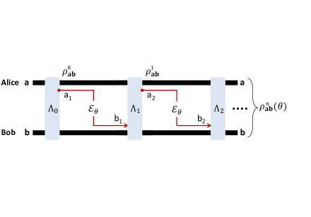
Figure 1: Arbitrary adaptive protocol for quantum parameter estimation. After preparation of the register state $\rho_{\mathbf{ab}}^{0}$ by means of an initial QO $\Lambda_{0}$, Alice starts probing the box $\{\mathcal{E}_{\theta}\}$ by sending a system $a_{1}$ from her register, with Bob getting the output $b_{1}$. This is repeated$\ n$ times with each transmission $a_{i}\rightarrow b_{i}$ interleaved by two QOs $\Lambda_{i-1}$ and $\Lambda_{i}$. The output state $\rho_{\mathbf{ab}}^{n}(\theta)$ is finally subject to an optimal measurement.

The final step consists of measuring the output state. The outcome is processed into an unbiased estimator of $\theta$, with an associated protocol-dependent QFI

$$I_{\theta}^{n}(\mathcal{P})=\frac{8\left\{1-F[\rho_{\mathbf{ab}}^{n}(\theta),\rho_{\mathbf{ab}}^{n}(\theta+d\theta)]\right\}}{d\theta^{2}},$$ (1)

with $F(\rho,\sigma):=\mathrm{Tr}\sqrt{\sqrt{\sigma}\rho\sqrt{\sigma}}$ being the fidelity BuresFID . By optimizing over all adaptive protocols, we define the adaptive QFI $\bar{I}_{\theta}^{n}:=\sup_{\mathcal{P}}I_{\theta}^{n}(\mathcal{P})$, so that the minimum error-variance in the estimation of $\theta$ satisfies the quantum Cramer-Rao bound (QCRB) Sam1 ; Sam2 $\mathrm{Var}(\theta)\geq 1/\bar{I}_{\theta}^{n}$.

Teleportation stretching for quantum metrology.– We now compute the adaptive QFI. Consider the class of teleportation-covariant channels in arbitrary dimension as generally defined in Ref. PLOB . They correspond to those quantum channels commuting with the random unitaries induced by teleportation, which are Pauli operators at finite dimension and displacement operators at infinite dimension telereview ; teleBennett ; Samtele . By definition, a quantum channel $\mathcal{E}$ is called “teleportation-covariant” if, for any teleportation unitary $U$ we may write PLOB

$$\mathcal{E}(U\rho U^{\dagger})=V\mathcal{E}(\rho)V^{\dagger},$$ (2)

for some other unitary $V$. This is a common property, owned by Pauli, erasure, and bosonic Gaussian channels.

Because of Eq. (2), we can simulate the channel $\mathcal{E}$ via local operations and classical communication (LOCC) applied to a suitable resource state. In fact, as explained in Fig. 2(i-ii), channel $\mathcal{E}$ can be simulated by a teleportation LOCC $\mathcal{T}$ performed over the channel’s Choi matrix $\rho_{\mathcal{E}}$, i.e., we may write PLOB

$$\mathcal{E}(\rho)=\mathcal{T}(\rho\otimes\rho_{\mathcal{E}}).$$ (3)

This simulation is intended to be asymptotic for bosonic channels PLOB . We consider $\mathcal{E}(\rho)=\lim_{\mu}\mathcal{T}_{\mu}(\rho\otimes\rho_{\mathcal{E}}^{\mu})$, where $\mathcal{T}_{\mu}$ is a sequence of teleportation LOCCs and $\rho_{\mathcal{E}}^{\mu}:=\mathcal{I}\otimes\mathcal{E}(\Phi^{\mu})$ is a sequence computed on two-mode squeezed vacuum (TMSV) states $\Phi^{\mu}$ WeeRMP , so that $\Phi:=\lim_{\mu}\Phi^{\mu}$ defines the asymptotic Einstein-Podolsky-Rosen (EPR) state and $\rho_{\mathcal{E}}:=\lim_{\mu}\rho_{\mathcal{E}}^{\mu}$ defines the asymptotic Choi matrix PLOB . In the following, for any pair of asymptotic states $\rho_{0,1}:=\lim_{\mu}\rho_{0,1}^{\mu}$, we correspondingly extend a functional $f$ to the limit as $f(\rho_{0},\rho_{1}):=\lim_{\mu}f(\rho_{0}^{\mu},\rho_{1}^{\mu})$.

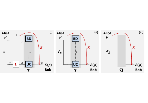
Figure 2: Teleportation covariance and channel simulation. In panel (i), we consider a teleportation-covariant channel $\mathcal{E}$ (red curvy line) from Alice’s system $a$ to Bob’s system $b$. This can be simulated by teleporting system $a$ to system $C$, by means of a maximally-entangled state $\Phi_{AC}$ and a Bell detection (BD) on systems $a$ and $A$, with outcome $k$. System $C$ is projected onto a state $\rho_{C}$ which is equal to $\rho_{a}$ up to a teleportation unitary $U_{k}$. Because of Eq. (2), we now have $\rho_{B}=\mathcal{E}(\rho_{C})=\mathcal{E}(U_{k}\rho_{a}U_{k}^{\dagger})=V_{k}\mathcal{E}(\rho_{a})V_{k}^{\dagger}$ for some other unitary $V_{k}$. Upon receiving $k$ from Alice, Bob may undo $V_{k}$ on system $B$ by applying a unitary correction (UC) $V_{k}^{-1}$. Thus, he retrieves the output state $\rho_{b}=\mathcal{E}(\rho_{a})$. Overall, Alice’s BD and Bob’s UC represent a teleportation LOCC $\mathcal{T}$. As shown in panel (ii), this is equivalent to simulate the channel by teleporting  the state over the channel’s Choi matrix $\rho_{\mathcal{E}}:=\mathcal{I}\otimes\mathcal{E}(\Phi)$, so that we may write Eq. (3). The teleportation simulation $(\mathcal{T},\rho_{\mathcal{E}})$ becomes asymptotic $(\mathcal{T}_{\mu},\rho_{\mathcal{E}}^{\mu})$ for bosonic channels. By comparing with panel (iii), we see that we have provided a computable design for the tool of quantum simulation Gatearray ; Qsim0 ; Qsim , reducing the quantum operation $\mathcal{U}$ to a teleportation LOCC $\mathcal{T}$, and the (difficult-to-find) programme state $\sigma_{\mathcal{E}}$ to the channel’s Choi matrix $\rho_{\mathcal{E}}$.

The teleportation-based simulation provides a powerful design to the generic tool of quantum simulation Gatearray ; Qsim0 ; Qsim which is described by

$$\mathcal{E}(\rho)=\mathcal{U}(\rho\otimes\sigma_{\mathcal{E}}),$$ (4)

where $\mathcal{U}$ is a trace-preserving QO parameterU and $\sigma_{\mathcal{E}}$ is some programme state, as in Fig. 2(iii). First of all, we establish a simple criterion (teleportation covariance) that allows us to identify channels $\mathcal{E}$ that are simulable as in Eq. (3) and, therefore, programmable as in Eq. (4). Then, we give an explicit solution to Eq. (4), so that $\mathcal{U}$ reduces to teleportation and the programme state $\sigma_{\mathcal{E}}$ is found to be the channel’s Choi matrix (see Fig. 2). As we will see below, this insight drastically simplifies computations.

For a channel which is “Choi-stretchable” as in Eq. (3), we may apply teleportation stretching PLOB ; Network . After stretching, the output $\rho_{\mathbf{ab}}^{n}$ of an adaptive protocol for quantum/private communication takes the form

$$\rho_{\mathbf{ab}}^{n}=\bar{\Lambda}(\rho_{\mathcal{E}}^{\otimes n}),$$ (5)

where $\bar{\Lambda}$ is trace-preserving LOCC Note . Here, to simplify quantum metrology, we do not need to enforce the LOCC structure, so that $\bar{\Lambda}$ may be an arbitrary CPTP map. In this sense the following lemma provides a full adaptation of the tool for the task of parameter estimation Appendix .

Lemma 1 (stretching of adaptive metrology)

Consider the adaptive estimation of the parameter $\theta$ of a teleportation-covariant channel $\mathcal{E}_{\theta}$. After $n$ probings, the output of the adaptive protocol can be written as

$$\rho_{\mathbf{ab}}^{n}(\theta)=\bar{\Lambda}\left(\rho_{\mathcal{E}_{\theta}}^{\otimes n}\right)=\lim_{\mu}\bar{\Lambda}_{\mu}(\rho_{\mathcal{E}_{\theta}}^{\mu\otimes n}),$$ (6)

where $\bar{\Lambda}$ is a $\theta$-independent CPTP map and $\rho_{\mathcal{E}_{\theta}}$ is the channel’s Choi matrix. If channel $\mathcal{E}_{\theta}$ is bosonic, then the decomposition is asymptotic $(\bar{\Lambda}_{\mu},\rho_{\mathcal{E}_{\theta}}^{\mu})$ with a sequence of CPTP maps $\bar{\Lambda}_{\mu}$ and Choi-approximating states $\rho_{\mathcal{E}_{\theta}}^{\mu}$.

By exploiting Lemma 1, we now show that the adaptive estimation of noise in teleportation-covariant channels cannot exceed the SQL, and can always be reduced to non-adaptive strategies. In fact, we have the following no-go theorem from teleportation Appendix .

Theorem 2 (No-go: tele-covariance implies SQL)

The adaptive estimation of the noise parameter $\theta$ of a teleportation-covariant channel $\mathcal{E}_{\theta}$ satisfies the QCRB $\mathrm{Var}(\theta)\geq 1/\bar{I}_{\theta}^{n}$, where the adaptive QFI takes the form

$$\bar{I}_{\theta}^{n}=nB(\rho_{\mathcal{E}_{\theta}}),~{}~{}B(\rho_{\mathcal{E}_{\theta}}):=\frac{8\left[1-F(\rho_{\mathcal{E}_{\theta}},\rho_{\mathcal{E}_{\theta+d\theta}})\right]}{d\theta^{2}}.$$ (7)

For large $n$, the QCRB is achievable by entanglement-based non-adaptive protocols. For bosonic channels, we implicitly assume $F(\rho_{\mathcal{E}_{\theta}},\rho_{\mathcal{E}_{\theta+d\theta}}):=\lim_{\mu}F(\rho_{\mathcal{E}_{\theta}}^{\mu},\rho_{\mathcal{E}_{\theta+d\theta}}^{\mu})$.

There are two important aspects in this theorem. The first is the achievability of the bound Achievability . The second is the extreme simplification of the adaptive QFI, which becomes a functional of the channel’s Choi matrix, computable almost instantaneously for many channels. Because the QFI takes such a simple form, our results are easily extended to bosonic channels lossnoise and can also be generalized to multiparameter estimation Appendix . The teleportation-based approach is so powerful that it is an open problem to find other channels (e.g., programmable) for which we may compute the adaptive QFI beyond the class of teleportation-covariant channels.

Analytical formulas.–  Let us use Theorem 2 to study the adaptive estimation of error probabilities in qubit channels Nielsen . For a depolarizing channel with probability $p$ we find the asymptotically achievable bound Appendix

$$\mathrm{Var}(p)\geq p(1-p)/n.$$ (8)

This result is also valid for the adaptive estimation of the probability $p$ of a dephasing channel or an erasure channel Appendix . Thus we show that the bounds of Refs. Qsim ; RafaComms are adaptive in a straightforward way.

Now consider a bosonic Gaussian channel which transforms input quadratures WeeRMP $\hat{x}=(\hat{q},\hat{p})^{T}$ as $\hat{x}\rightarrow\eta\hat{x}+|1-\eta|\hat{x}_{T}+\xi$, where $\eta$ is a real gain parameter, $\hat{x}_{T}$ are the quadratures of a thermal environment with $\bar{n}_{T}$ mean number of photons, and $\xi$ is an additive Gaussian noise variable with variance $w$. A specific case is the thermal-loss channel for which $0\leq\eta<1$ and $\xi=0$. It is immediate to compute the ultimate (adaptive) limit for estimating thermal noise $\bar{n}_{T}>0$ in such a channel. By using our Theorem 2 and the formula for the fidelity between multimode Gaussian states Banchi , we easily derive Appendix

$$\mathrm{Var}(\bar{n}_{T})\geq\bar{n}_{T}(\bar{n}_{T}+1)/n,$$ (9)

which is achievable for large $n$.

The latter result sets the ultimate precision for estimating the excess (thermal) noise in a tapped communication line QKD or the temperature of a quasi-monochromatic bosonic bath. Eq. (9) is also valid for estimating thermal noise in an amplifier, defined by $\eta>1$ and $\xi=0$. Finally, for $\eta=1$ and $\xi\neq 0$, we have an additive-noise Gaussian channel. The adaptive estimation of its variance $w>0$ is limited by Appendix

$$\mathrm{Var}(w)\geq w^{2}/n.$$ (10)

Adaptive quantum channel discrimination.–  We can simplify other types of adaptive protocols whose performance is quantified by functionals which are monotonic under CPTP maps MethodsNOTA . Thus, consider a box with two equiprobable channels $\{\mathcal{E}_{k}\}=\{\mathcal{E}_{0},\mathcal{E}_{1}\}$. An adaptive discrimination protocol $\mathcal{P}$ consists of local registers prepared in a state $\rho_{\mathbf{ab}}^{0}$, which are then used to probe the box $n$ times while being assisted by a sequence of QOs $\mathcal{P}$, similar to Fig. 1. The output state $\rho_{\mathbf{ab}}^{n}(k)$ is optimally measured Hesltrom so that we may write the protocol-dependent error probability in terms of the trace distance $D$

$$p(k^{\prime}\neq k|\mathcal{P})=\frac{1-D[\rho_{\mathbf{ab}}^{n}(0),\rho_{\mathbf{ab}}^{n}(1)]}{2}.$$ (11)

The ultimate error probability is given by optimizing over all adaptive protocols, i.e., $p_{\mathrm{err}}:=\inf_{\mathcal{P}}p(k^{\prime}\neq k|\mathcal{P})$.

For the discrimination of teleportation-covariant channels, we may write the output state $\rho_{\mathbf{ab}}^{n}(k)$ using the same Choi decomposition of Eq. (6), proviso that we replace $\rho_{\mathcal{E}_{\theta}}$ with its discrete version $\rho_{\mathcal{E}_{k}}$, i.e.,

$$\rho_{\mathbf{ab}}^{n}(k)=\bar{\Lambda}\left(\rho_{\mathcal{E}_{k}}^{\otimes n}\right),$$ (12)

understood to be asymptotic for bosonic channels. We then prove Appendix the following result which expresses $p_{\mathrm{err}}$ in terms of the trace distance between Choi matrices.

Theorem 3

Consider an adaptive protocol for discriminating two teleportation-covariant channels $\{\mathcal{E}_{0},\mathcal{E}_{1}\}$. After $n$ probings, the minimum error probability is

$$p_{\mathrm{err}}=\frac{1-D(\rho_{\mathcal{E}_{0}}^{\otimes n},\rho_{\mathcal{E}_{1}}^{\otimes n})}{2},$$ (13)

where $D=\lim_{\mu}D[\rho_{\mathcal{E}_{0}}^{\mu\otimes n},\rho_{\mathcal{E}_{1}}^{\mu\otimes n}]$ for bosonic channels.

For programmable channels $\{\mathcal{E}_{k}\}$ with states $\{\sigma_{\mathcal{E}_{k}}\}$, we may only write the bound $p_{\mathrm{err}}\geq[1-D(\sigma_{\mathcal{E}_{0}}^{\otimes n},\sigma_{\mathcal{E}_{1}}^{\otimes n})]/2$. In general, this is not achievable because we do not know if $\sigma_{\mathcal{E}_{k}}$ can be generated by transmission through $\mathcal{E}_{k}$. By contrast, for teleportation-covariant channels, the bound is always achievable and the optimal strategy is non-adaptive, based on sending parts of maximally-entangled states and then measuring the output Choi matrices. Because of the equality in Eq. (13) we may write both lower and upper (single-letter) bounds. Using the Fuchs-van der Graaf relations Fuchs , the quantum Pinsker’s inequality Pinsker ; Lieb , and the quantum Chernoff bound (QCB) QCB1 , we find that the adaptive discrimination of teleportation-covariant channels must satisfy Appendix

$$\frac{1-\sqrt{\min\left\{1-F^{2n},nS\right\}}}{2}\leq p_{\mathrm{err}}\leq\frac{Q^{n}}{2}\leq\frac{F^{n}}{2},$$ (14)

where $F:=F(\rho_{\mathcal{E}_{0}},\rho_{\mathcal{E}_{1}})$, $Q:=\inf_{s}\mathrm{Tr}(\rho_{\mathcal{E}_{0}}^{s},\rho_{\mathcal{E}_{1}}^{1-s})$ and $S:=(\ln\sqrt{2})\min\{S(\rho_{\mathcal{E}_{0}}||\rho_{\mathcal{E}_{1}}),S(\rho_{\mathcal{E}_{1}}||\rho_{\mathcal{E}_{0}})\}$, with $S(\rho||\sigma)$ being the relative entropy VedralRMP . Here recall that the QCB is tight for large $n$ QCB1 , so that $p_{\mathrm{err}}\simeq Q^{n}/2$. All these functionals are asymptotic for bosonic channels.

In particular, for two thermal-loss channels with identical transmissivity but different thermal noise, $\bar{n}_{0}$ and $\bar{n}_{1}$, we may take the limit and compute Appendix

$$Q=\inf_{s}\left[(\bar{n}_{0}+1)^{s}(\bar{n}_{1}+1)^{1-s}-\bar{n}_{0}^{s}\bar{n}_{1}^{1-s}\right]^{-1}.$$ (15)

For these channels, it is interesting to study the infinitesimal discrimination $\bar{n}_{0}=\bar{n}_{T}$ and $\bar{n}_{1}=\bar{n}_{T}+d\bar{n}_{T}$. As we show in a lemma Appendix , when we consider the discrimination of two infinitesimally-close states, $\rho_{\theta}$ and $\rho_{\theta+d\theta}$, the $n$-copy minimum error probability can be connected with the QCRB for estimating parameter $\theta$. Applying this result to the asymptotic Choi matrices of the thermal-loss channels and taking the limit of large $n$, we get Appendix $p_{\mathrm{err}}\simeq e^{-n\Sigma}/2$ where $\Sigma=[8\bar{n}_{T}(\bar{n}_{T}+1)]^{-1}d\bar{n}_{T}^{2}$ for $\bar{n}_{T}>0$. For the specific case of $\bar{n}_{T}=0$ (infinitesimal discrimination from vacuum noise), we have a discontinuity and we may write $\Sigma=d\bar{n}_{T}$ Appendix . These results represent the ultimate adaptive limits for resolving two temperatures, e.g., for testing the Unruh effect field1 or the Hawking radiation in analogue systems field2 .

Conclusions.–  In this paper we have established the ultimate limits of adaptive noise estimation and discrimination for the wide class of teleportation-covariant channels, which includes fundamental transformations for qubits, qudits and bosonic systems. We have reduced the most general adaptive protocols for parameter estimation and channel discrimination into much simpler block versions, where the output states are simply expressed in terms of Choi matrices of the encoding channels. This allowed us to prove that the optimal noise estimation of teleportation-covariant channels scales as the SQL and is fully determined by their Choi matrices. Our work not only shows that teleportation is a primitive for quantum metrology but also provides remarkably simple and practical results, such as the precision limit for estimating the excess noise of a thermal-loss channel, which is a basic channel in continuous variable QKD. Setting the ultimate precision limits of noise estimation and discrimination has broad implications, e.g., in quantum tomography, imaging, sensing and even for testing quantum field theories in non-inertial frames.

Acknowledgments.–  This work was supported by the UK Quantum Communications hub (EP/M013472/1) and the Innovation Fund Denmark (Qubiz project). The authors thank S. Lloyd, S. L. Braunstein, R. Laurenza, L. Maccone, R. Demkowicz-Dobrzanski, D. Braun, and J. Kolodynski for comments and discussions.

Note added.–  While completing the final revision of this work, a follow-up Copy appeared on the arXiv AddedNOTE .

Supplemental Material

I Teleportation stretching of adaptive quantum metrology (proof of Lemma 1)

Here we explicitly show how to “stretch” an adaptive protocol of parameter estimation into a block form. This is a simple adaptation of the general argument that Ref. PLOBapp originally provided for protocols of quantum/private communication. We first consider discrete-variable channels and then we extend the results to continuous-variable channels afterwards. The procedure is explained in Fig. 3 for the $i$th transmission through an arbitrary teleportation-covariant channel $\mathcal{E}$. As we can see, the register state of the two parties is updated by the recursive formula

$$\rho_{\mathbf{ab}}^{i}=\Delta_{i}(\rho_{\mathcal{E}}\otimes\rho_{\mathbf{ab}}^{i-1}),$$ (16)

for some quantum operation (QO) $\Delta_{i}$. Iterating this formula for $n$ transmissions, we accumulate $n$ Choi matrices $\rho_{\mathcal{E}}^{\otimes n}$ while collapsing the QOs. In our estimation protocol, after $n$ probings of the channel $\mathcal{E}_{\theta}$, the register state becomes

$$\rho_{\mathbf{ab}}^{n}(\theta)=\Delta\left(\rho_{\mathcal{E}_{\theta}}^{\otimes n}\otimes\rho_{\mathbf{ab}}^{0}\right),$$ (17)

where $\Delta=\Lambda_{n}\circ\cdots\circ\Lambda_{1}$ does not depend on $\theta$.

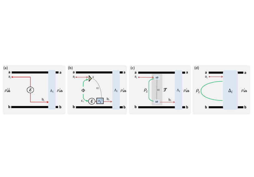
Figure 3: Teleportation stretching of an adaptive protocol. (a) Consider the $i$th transmission $a_{i}\rightarrow b_{i}$ through a teleportation-covariant channel $\mathcal{E}$, followed by the QO $\Lambda_{i}$, so that the register state $\rho_{\mathbf{ab}}^{i-1}:=\rho_{\mathbf{a}a_{i}\mathbf{b}}$ is updated to $\rho_{\mathbf{ab}}^{i}$. (b) We can replace the actual transmission with quantum teleportation. The input system $a_{i}$ and part of a maximally-entangled state $\Phi$ are subject to a Bell detection with outcome $k$. This process teleports the reduced state $\rho_{a_{i}}$ of $a_{i}$ onto system $c_{i}$ up to a unitary operator $U_{k}$. Because the channel is teleportation-covariant, we have $\mathcal{E}(U_{k}\rho_{a_{i}}U_{k}{}^{\dagger})=V_{k}\mathcal{E}(\rho_{a_{i}})V_{k}^{\dagger}$ so that $V_{k}$ can be undone at the output, and we retrieve $\mathcal{E}(\rho_{a_{i}})$ on system $b_{i}$. This process also teleports all the correlations that system $a_{i}$ may have with other systems in the registers, i.e., it teleports part $a_{i}$ of the input state $\rho_{\mathbf{a}a_{i}\mathbf{b}}$. (c) Note that the propagation of $\Phi$ through channel $\mathcal{E}$ defines its Choi matrix $\rho_{\mathcal{E}}$, and the teleportation process over this state is just an LOCC, that becomes trace-preserving after averaging over the Bell outcomes. In other words, we may write $\mathcal{E}(\rho_{a_{i}})=\mathcal{T}(\rho_{a_{i}}\otimes\rho_{\mathcal{E}})$ for a teleportation LOCC $\mathcal{T}$. This is a particular case of Choi-stretchable channel as generally defined in Ref. PLOBapp . Including the registers, we may write $\mathcal{I}_{\mathbf{a}}\otimes\mathcal{E}\otimes\mathcal{I}_{\mathbf{b}}(\rho_{\mathbf{a}a_{i}\mathbf{b}})=\mathcal{I}_{\mathbf{a}}\otimes\mathcal{T}\otimes\mathcal{I}_{\mathbf{b}}(\rho_{\mathbf{a}a_{i}\mathbf{b}}\otimes\rho_{\mathcal{E}})$.  (d) We finally collapse $\mathcal{I}_{\mathbf{a}}\otimes\mathcal{T}\otimes\mathcal{I}_{\mathbf{b}}$ and $\Lambda_{i}$ into a single QO $\Delta_{i}$ applied to $\rho_{\mathbf{a}a_{i}\mathbf{b}}\otimes\rho_{\mathcal{E}}$, so that we can write the recursive formula of Eq. (16).

In Eq. (17), we may include the initial register state $\rho_{\mathbf{ab}}^{0}$ into $\Delta$ and write

$$\rho_{\mathbf{ab}}^{n}(\theta)=\bar{\Lambda}\left(\rho_{\mathcal{E}_{\theta}}^{\otimes n}\right),$$ (18)

for a trace-preserving and $\theta$-independent QO $\bar{\Lambda}$ (trace-preserving is assured by averaging over all measurements involved in the teleportation simulation and the original adaptive protocol).

Note that we may repeat the reasoning in Fig. 3 for a programmable channel $\mathcal{E}$, which can be represented as in Fig. 3(c) but with an arbitrary trace-preserving QO $\mathcal{U}$ (in the place of the teleportation LOCC) applied to some programme state $\sigma_{\mathcal{E}}$ (in the place of the Choi matrix $\rho_{\mathcal{E}}$). This leads to a different form of Eq. (18), namely

$$\rho_{\mathbf{ab}}^{n}(\theta)=\tilde{\Lambda}\left(\sigma_{\mathcal{E}_{\theta}}^{\otimes n}\right),$$ (19)

for some other trace-preserving and $\theta$-independent QO $\tilde{\Lambda}$.

Extension to bosonic channels

For a bosonic teleportation-covariant channel, we need to consider an asymptotic simulation. In other words, we start from the imperfect simulation $\mathcal{E}^{\mu}(\rho)=\mathcal{T}^{\mu}(\rho\otimes\rho_{\mathcal{E}}^{\mu})$ where the teleportation LOCC $\mathcal{T}^{\mu}$ is built considering a finite-energy POVM $\mathcal{B}^{\mu}$ (such that the ideal Bell detection is defined as the limit $\mathcal{B}:=\lim_{\mu}\mathcal{B}^{\mu}$) and $\rho_{\mathcal{E}}^{\mu}:=\mathcal{I}\otimes\mathcal{E}(\Phi^{\mu})$ defines the bosonic Choi matrix as $\rho_{\mathcal{E}}:=\lim_{\mu}\rho_{\mathcal{E}}^{\mu}$. Because of the Braunstein-Kimble protocol Samteleapp ; DAriano , for any bipartite state $\rho$, we have the point-wise limit

$$\|\mathcal{I}\otimes\mathcal{E}(\rho)-\mathcal{I}\otimes\mathcal{E}^{\mu}(\rho)\|_{1}\overset{\mu}{\rightarrow}0~{}.$$ (20)

This limit can equivalently be expressed in terms of bounded diamond norm. In fact, let us consider the (compact) set of energy-constrained bipartite states $\mathcal{D}_{N}:=\{\rho~{}|~{}\mathrm{Tr}(\hat{N}\rho)\leq N\}$, where $\hat{N}$ is the total number operator. Then, for two bosonic channels, $\mathcal{E}_{1}$ and $\mathcal{E}_{2}$, one may define the bounded diamond norm PLOBapp

$$\left\|\mathcal{E}_{1}-\mathcal{E}_{2}\right\|_{\diamond N}:=\sup_{\rho\in\mathcal{D}_{N}}\|\mathcal{I}\otimes\mathcal{E}_{1}(\rho)-\mathcal{I}\otimes\mathcal{E}_{2}(\rho)\|_{1}~{},$$ (21)

which provides the standard (unbounded) diamond norm Paulsenapp in the limit of large $N$, i.e.,

$$\left\|\mathcal{E}_{1}-\mathcal{E}_{2}\right\|_{\diamond}:=\lim_{N\rightarrow\infty}\left\|\mathcal{E}_{1}-\mathcal{E}_{2}\right\|_{\diamond N}~{}.$$ (22)

By exploiting the fact that $\mathcal{D}_{N}$ is a compact set, the pointwise limit in Eq. (20) implies the uniform limit

$$\left\|\mathcal{E}-\mathcal{E}^{\mu}\right\|_{\diamond N}\overset{\mu}{\rightarrow}0\text{~{}~{}{for any }}N.$$ (23)

Therefore, for any $N<\infty$ and $\varepsilon>0$, there is a sufficiently large $\mu$ such that $\|\mathcal{E}-\mathcal{E}^{\mu}\|_{\diamond N}\leq\varepsilon$. For the estimation protocol this happens for any $\theta$, so that we may write

$$\|\mathcal{E}_{\theta}-\mathcal{E}_{\theta}^{\mu}\|_{\diamond N}\leq\varepsilon~{}.$$ (24)

The latter bound can be extended to the output of the adaptive protocol after $n$ channel uses. Consider the original output state

$$\rho_{\mathbf{ab}}^{n}(\theta):=\Lambda_{n}\circ\mathcal{E}_{\theta}\circ\Lambda_{n-1}\cdots\circ\mathcal{E}_{\theta}(\rho_{\mathbf{ab}}^{0}),$$ (25)

and its simulation

$$\rho_{\mathbf{ab}}^{n,\mu}(\theta):=\Lambda_{n}\circ\mathcal{E}_{\theta}^{\mu}\circ\Lambda_{n-1}\cdots\circ\mathcal{E}_{\theta}^{\mu}(\rho_{\mathbf{ab}}^{0}),$$ (26)

which is found by replacing $\mathcal{E}_{\theta}$ with $\mathcal{E}_{\theta}^{\mu}$. Here it is understood that $\mathcal{E}_{\theta}$ and $\mathcal{E}_{\theta}^{\mu}$ are applied to system $a_{i}$ for the $i$-th transmission, i.e., we have $\mathcal{E}_{\theta}=\mathcal{I}_{\mathbf{a}}\otimes(\mathcal{E}_{\theta})_{a_{i}}\otimes\mathcal{I}_{\mathbf{b}}$. Assume that the mean total number of photons in the states $\rho_{\mathbf{ab}}^{n}(\theta)$ and $\rho_{\mathbf{ab}}^{n,\mu}(\theta)$ is bounded by some large but finite value $N(n)$ for any $\theta$ and $\mu$. Since these are physical states, it is always possible to find such a common bound. In general, for $n$ uses, we have a sequence $\{N(0),\cdots,N(i),\cdots,N(n)\}$ of which $N(n)$ can always be chosen to be the greatest value.

Then, we may show that

$$\|\rho_{\mathbf{ab}}^{n}(\theta)-\rho_{\mathbf{ab}}^{n,\mu}(\theta)\|_{1}\leq n\left\|\mathcal{E}_{\theta}-\mathcal{E}_{\theta}^{\mu}\right\|_{\diamond N(n)}~{}.$$ (27)

In fact, for $n=2$, we may write

$$\|\rho_{\mathbf{ab}}^{2}(\theta)-\rho_{\mathbf{ab}}^{2,\mu}(\theta)\|_{1} =\|\Lambda_{2}\circ\mathcal{E}_{\theta}\circ\Lambda_{1}\circ\mathcal{E}_{\theta}(\rho_{\mathbf{ab}}^{0})-\Lambda_{2}\circ\mathcal{E}_{\theta}^{\mu}\circ\Lambda_{1}\circ\mathcal{E}_{\theta}^{\mu}(\rho_{\mathbf{ab}}^{0})\|_{1}$$

$$\overset{(1)}{\leq}\|\mathcal{E}_{\theta}\circ\Lambda_{1}\circ\mathcal{E}_{\theta}(\rho_{\mathbf{ab}}^{0})-\mathcal{E}_{\theta}^{\mu}\circ\Lambda_{1}\circ\mathcal{E}_{\theta}^{\mu}(\rho_{\mathbf{ab}}^{0})\|_{1}$$

$$\overset{(2)}{\leq}\|\mathcal{E}_{\theta}\circ\Lambda_{1}\circ\mathcal{E}_{\theta}(\rho_{\mathbf{ab}}^{0})-\mathcal{E}_{\theta}\circ\Lambda_{1}\circ\mathcal{E}_{\theta}^{\mu}(\rho_{\mathbf{ab}}^{0})\|_{1}+\|\mathcal{E}_{\theta}\circ\Lambda_{1}\circ\mathcal{E}_{\theta}^{\mu}(\rho_{\mathbf{ab}}^{0})-\mathcal{E}_{\theta}^{\mu}\circ\Lambda_{1}\circ\mathcal{E}_{\theta}^{\mu}(\rho_{\mathbf{ab}}^{0})\|_{1}$$

$$\overset{(3)}{\leq}\|\mathcal{E}_{\theta}(\rho_{\mathbf{ab}}^{0})-\mathcal{E}_{\theta}^{\mu}(\rho_{\mathbf{ab}}^{0})\|_{1}+\|\mathcal{E}_{\theta}[\Lambda_{1}\circ\mathcal{E}_{\theta}^{\mu}(\rho_{\mathbf{ab}}^{0})]-\mathcal{E}_{\theta}^{\mu}[\Lambda_{1}\circ\mathcal{E}_{\theta}^{\mu}(\rho_{\mathbf{ab}}^{0})]\|_{1}$$

$$\overset{(4)}{\leq}2\left\|\mathcal{E}_{\theta}-\mathcal{E}_{\theta}^{\mu}\right\|_{\diamond N(n)}~{},$$ (28)

where: (1) we use the monotonicity under completely-positive trace-preserving (CPTP) maps (note that the QO $\Lambda_{2}$ can always be made trace-preserving by adding ancillas and delaying quantum measurements at the end of the protocol); (2) we use the triangle inequality; (3) we use monotonicity with respect to $\mathcal{E}_{\theta}\circ\Lambda_{1}$; and (4) we upperbound the trace distance via the bounded diamond norm. Extension of Eq. (28) to arbitrary $n$ is just a matter of technicalities.

From Eq. (24) we have that, for any finite $N(n)$ and $\varepsilon>0$, there is a sufficiently large $\mu$ such that

$$\left\|\mathcal{E}_{\theta}-\mathcal{E}_{\theta}^{\mu}\right\|_{\diamond N(n)}\leq\varepsilon~{}.$$ (29)

Combining the latter with Eq. (27) leads to

$$\|\rho_{\mathbf{ab}}^{n}(\theta)-\rho_{\mathbf{ab}}^{n,\mu}(\theta)\|_{1}\leq n\varepsilon~{}.$$ (30)

By using a finite-energy simulation $\mathcal{T}^{\mu}$, we may may weaken Eq. (18) into

$$\rho_{\mathbf{ab}}^{n,\mu}(\theta)=\bar{\Lambda}_{\mu}\left(\rho_{\mathcal{E}_{\theta}}^{\mu\otimes n}\right),$$ (31)

where the $\theta$-independent QO $\bar{\Lambda}_{\mu}$ is determined by the original QOs of the protocol plus the teleportation LOCCs $\mathcal{T}^{\mu}$ ($\bar{\Lambda}_{\mu}$ is trace-preserving by averaging over all measurements). Thus, combining Eqs. (30) and (31), we find that

$$\|\rho_{\mathbf{ab}}^{n}(\theta)-\bar{\Lambda}_{\mu}\left(\rho_{\mathcal{E}_{\theta}}^{\mu\otimes n}\right)\|_{1}\leq n\varepsilon.$$ (32)

or, equivalently, $\|\rho_{\mathbf{ab}}^{n}(\theta)-\bar{\Lambda}_{\mu}\left(\rho_{\mathcal{E}_{\theta}}^{\mu\otimes n}\right)\|_{1}\overset{\mu}{\rightarrow}0$. Therefore, given an adaptive protocol with arbitrary register energy $N(n)$, we may write its $n$-use output state as the (trace-norm) limit

$$\rho_{\mathbf{ab}}^{n}(\theta)=\lim_{\mu}\bar{\Lambda}_{\mu}\left(\rho_{\mathcal{E}_{\theta}}^{\mu\otimes n}\right).$$ (33)

II No-go: teleportation-covariance implies SQL (proof of Theorem 2)

First consider discrete-variable teleportation-covariant channels $\mathcal{E}_{\theta}$. Let us adopt the following notation

$$B(n,\theta):=\frac{8(1-F_{\theta}^{n})}{d\theta^{2}},~{}~{}F_{\theta}:=F(\rho_{\mathcal{E}_{\theta}},\rho_{\mathcal{E}_{\theta+d\theta}}).$$ (34)

We first show that $B(n,\theta)$ is an upper bound for $\bar{I}_{\theta}^{n}$. Given any adaptive protocol $\mathcal{P}$, we may write $\rho_{\mathbf{ab}}^{n}(\theta)=\bar{\Lambda}\left(\rho_{\mathcal{E}_{\theta}}^{\otimes n}\right)$ with a $\theta$-independent QO $\bar{\Lambda}$. In particular, this means that we may also write

$$\rho_{\mathbf{ab}}^{n}(\theta+d\theta)=\bar{\Lambda}\left(\rho_{\mathcal{E}_{\theta+d\theta}}^{\otimes n}\right).$$ (35)

In order to bound the quantum Fisher information (QFI)

$$I_{\theta}^{n}(\mathcal{P})=\frac{8\left\{1-F[\rho_{\mathbf{ab}}^{n}(\theta),\rho_{\mathbf{ab}}^{n}(\theta+d\theta)]\right\}}{d\theta^{2}},$$ (36)

we exploit basic properties of the quantum fidelity. In fact, we derive

$$F[\rho_{\mathbf{ab}}^{n}(\theta),\rho_{\mathbf{ab}}^{n}(\theta+d\theta)]\overset{(1)}{\geq}F(\rho_{\mathcal{E}_{\theta}}^{\otimes n},\rho_{\mathcal{E}_{\theta+d\theta}}^{\otimes n})\overset{(2)}{=}F(\rho_{\mathcal{E}_{\theta}},\rho_{\mathcal{E}_{\theta+d\theta}})^{n}:=F_{\theta}^{n},$$ (37)

where we use: (1) the monotonicity of the fidelity under CPTP maps, as is $\bar{\Lambda}$; and (2) its multiplicativity over tensor-product states. Therefore, by using Eq. (37) in Eq. (36), we derive $I_{\theta}^{n}(\mathcal{P})\leq B(n,\theta)$ for any protocol $\mathcal{P}$. The latter bound is also valid for the supremum over all protocols, therefore proving $\bar{I}_{\theta}^{n}\leq B(n,\theta)$.

The next step is to show that the bound $B(n,\theta)$ is additive. For $n=1$ and $d\theta\rightarrow 0$, we may write $F_{\theta}=1-B(1,\theta)d\theta^{2}/8$ which implies $F_{\theta}^{n}=1-nB(1,\theta)d\theta^{2}/8$ up to $O(d\theta^{4})$. The latter expansion leads to $B(n,\theta)=nB(1,\theta)$, so that we may directly write

$$\bar{I}_{\theta}^{n}\leq nB(1,\theta)=nB(\theta),~{}~{}B(\theta):=\frac{8(1-F_{\theta})}{d\theta^{2}}.$$ (38)

Consider now a non-adaptive protocol $\mathcal{\tilde{P}}$ where Alice prepares $n$ maximally-entangled (Bell) states $\Phi^{\otimes n}$ and partly propagates them through the box, so that the output is $\rho_{\mathbf{ab}}^{n}(\theta)=\rho_{\mathcal{E}_{\theta}}^{\otimes n}$. By replacing this state in Eq. (36), we get $I_{\theta}^{n}(\mathcal{\tilde{P}})=nB(\theta)$, so that $\bar{I}_{\theta}^{n}\geq nB(\theta)$. Combining the latter with Eq. (38) leads to $\bar{I}_{\theta}^{n}=nB(\theta)$. Since $\mathcal{\tilde{P}}$ uses independent probing states, the quantum Cramer Rao bound (QCRB) $\mathrm{Var}(\theta)\geq[I_{\theta}^{n}(\mathcal{\tilde{P}})]^{-1}=[nB(\theta)]^{-1}$ is asymptotically achievable (for large $n$) by using local measurements and adaptive estimators Gillapp .

For a programmable channel $\mathcal{E}_{\theta}$ with programme state $\sigma_{\mathcal{E}_{\theta}}$ we may write $\rho_{\mathbf{ab}}^{n}(\theta)=\tilde{\Lambda}\left(\sigma_{\mathcal{E}_{\theta}}^{\otimes n}\right)$, which leads to the following alternative version of Eq. (37)

$$F[\rho_{\mathbf{ab}}^{n}(\theta),\rho_{\mathbf{ab}}^{n}(\theta+d\theta)\geq F(\sigma_{\mathcal{E}_{\theta}},\sigma_{\mathcal{E}_{\theta+d\theta}})^{n}.$$ (39)

It is easy to repeat some of the previous steps to prove the bound

$$\bar{I}_{\theta}^{n}\leq n\frac{8\left[1-F(\sigma_{\mathcal{E}_{\theta}},\sigma_{\mathcal{E}_{\theta+d\theta}})\right]}{d\theta^{2}}.$$ (40)

However, we do not know if this bound is achievable or not, i.e., we cannot put an equality in Eq. (40), because we do not know if the programme state $\sigma_{\mathcal{E}_{\theta}}$ can be generated by the transmission of an input state through the channel.

Extension to bosonic channels

Let us consider continuous-variable teleportation-covariant channels. For any adaptive protocol $\mathcal{P}$, we may write

$$I_{\theta}^{n}(\mathcal{P}):=4\frac{d_{B}^{2}[\rho_{\mathbf{ab}}^{n}(\theta),\rho_{\mathbf{ab}}^{n}(\theta+d\theta)]}{d\theta^{2}},$$ (41)

where $d_{B}$ is the Bures distance

$$d_{B}(\rho_{1},\rho_{2})=\sqrt{2[1-F(\rho_{1},\rho_{2})]}.$$ (42)

The Bures distance between the output states, $\rho_{\mathbf{ab}}^{n}(\theta)$ and $\rho_{\mathbf{ab}}^{n}(\theta+d\theta)$, can be related to the Bures distance between the $\mu$-approximate output states, $\rho_{\mathbf{ab}}^{n,\mu}(\theta)$ and $\rho_{\mathbf{ab}}^{n,\mu}(\theta+d\theta)$. In fact, by applying the triangle inequality and bounding $d_{B}$ with the trace distance $D$, i.e.,

$$d_{B}^{2}(\rho_{1},\rho_{2})\leq D(\rho_{1},\rho_{2}):=\frac{1}{2}||\rho_{1}-\rho_{2}||_{1},$$ (43)

we get the following

$$d_{B}[\rho_{\mathbf{ab}}^{n}(\theta),\rho_{\mathbf{ab}}^{n}(\theta+d\theta)] \leq d_{B}[\rho_{\mathbf{ab}}^{n}(\theta),\rho_{\mathbf{ab}}^{n,\mu}(\theta)]+d_{B}[\rho_{\mathbf{ab}}^{n,\mu}(\theta),\rho_{\mathbf{ab}}^{n,\mu}(\theta+d\theta)]+d_{B}[\rho_{\mathbf{ab}}^{n,\mu}(\theta+d\theta),\rho_{\mathbf{ab}}^{n}(\theta+d\theta)]$$

$$\leq\sqrt{D[\rho_{\mathbf{ab}}^{n}(\theta),\rho_{\mathbf{ab}}^{n,\mu}(\theta)]}+d_{B}[\rho_{\mathbf{ab}}^{n,\mu}(\theta),\rho_{\mathbf{ab}}^{n,\mu}(\theta+d\theta)]+\sqrt{D[\rho_{\mathbf{ab}}^{n,\mu}(\theta+d\theta),\rho_{\mathbf{ab}}^{n}(\theta+d\theta)]}$$

$$\leq\sqrt{\frac{n}{2}\left\|\mathcal{E}_{\theta}-\mathcal{E}_{\theta}^{\mu}\right\|_{\diamond N(n)}}+d_{B}[\rho_{\mathbf{ab}}^{n,\mu}(\theta),\rho_{\mathbf{ab}}^{n,\mu}(\theta+d\theta)]+\sqrt{\frac{n}{2}\left\|\mathcal{E}_{\theta+d\theta}-\mathcal{E}_{\theta+d\theta}^{\mu}\right\|_{\diamond N(n)}}~{},$$ (44)

where, in the last step, we have also used Eq. (27) with $N(n)$ being the energy bound of protocol $\mathcal{P}$.

Using Eq. (29) we see that, for any energy-bounded protocol $\mathcal{P}$, there is a sufficiently large $\mu$ such that

$$d_{B}[\rho_{\mathbf{ab}}^{n}(\theta),\rho_{\mathbf{ab}}^{n}(\theta+d\theta)]\leq\sqrt{2n\varepsilon}+d_{B}[\rho_{\mathbf{ab}}^{n,\mu}(\theta),\rho_{\mathbf{ab}}^{n,\mu}(\theta+d\theta)].$$ (45)

In other words, we may write the following limit

$$d_{B}[\rho_{\mathbf{ab}}^{n}(\theta),\rho_{\mathbf{ab}}^{n}(\theta+d\theta)]\leq\lim_{\mu\rightarrow\infty}d_{B}[\rho_{\mathbf{ab}}^{n,\mu}(\theta),\rho_{\mathbf{ab}}^{n,\mu}(\theta+d\theta)],$$ (46)

which leads to

$$I_{\theta}^{n}(\mathcal{P})\leq\lim_{\mu\rightarrow\infty}I_{\theta}^{n,\mu}(\mathcal{P}),~{}~{}I_{\theta}^{n,\mu}(\mathcal{P}):=4\frac{d_{B}^{2}[\rho_{\mathbf{ab}}^{n,\mu}(\theta),\rho_{\mathbf{ab}}^{n,\mu}(\theta+d\theta)]}{d\theta^{2}}.$$ (47)

Now note that, at any finite $\mu$, we can use Eq. (31) and

$$\rho_{\mathbf{ab}}^{n,\mu}(\theta+d\theta)=\bar{\Lambda}_{\mu}\left(\rho_{\mathcal{E}_{\theta+d\theta}}^{\mu\otimes n}\right).$$ (48)

It is then easy to see that the derivation in Eq. (37) can be modified into

$$F[\rho_{\mathbf{ab}}^{n,\mu}(\theta),\rho_{\mathbf{ab}}^{n,\mu}(\theta+d\theta)]\geq(F_{\theta}^{\mu})^{n}:=F(\rho_{\mathcal{E}_{\theta}}^{\mu},\rho_{\mathcal{E}_{\theta+d\theta}}^{\mu})^{n}.$$ (49)

Therefore, for any energy-bounded protocol $\mathcal{P}$, we may write the following bound for the $\mu$-dependent QFI

$$I_{\theta}^{n,\mu}(\mathcal{P})\leq B(n,\theta,\mu):=\frac{8[1-(F_{\theta}^{\mu})^{n}]}{d\theta^{2}}.$$ (50)

As before, it is immediate to prove the additivity, so that we derive

$$I_{\theta}^{n,\mu}(\mathcal{P})\leq nB(\theta,\mu),~{}~{}B(\theta,\mu):=\frac{8\left[1-F(\rho_{\mathcal{E}_{\theta}}^{\mu},\rho_{\mathcal{E}_{\theta+d\theta}}^{\mu})\right]}{d\theta^{2}}~{}.$$ (51)

By taking the limit for large $\mu$ and optimizing over all $\mathcal{P}$, we therefore get

$$\bar{I}_{\theta}^{n}:=\sup_{\mathcal{P}}I_{\theta}^{n}(\mathcal{P})\leq\lim_{\mu\rightarrow\infty}nB(\theta,\mu)=n\frac{8\left[1-\lim_{\mu}F(\rho_{\mathcal{E}_{\theta}}^{\mu},\rho_{\mathcal{E}_{\theta+d\theta}}^{\mu})\right]}{d\theta^{2}}~{}.$$ (52)

Note that, because we consider a supremum in the definition of $\bar{I}_{\theta}^{n}$, we may also include the limit of energy-unbounded protocols. As a matter of fact, such asymptotic protocols are those saturating the upper bound. In fact, consider a non-adaptive protocol $\mathcal{\tilde{P}}_{\mu}$, where Alice transmits part of two-mode squeezed vacuum (TMSV) states $\Phi^{\mu\otimes n}$, so that the $n$-use output state is $\rho_{\mathbf{ab}}^{n}(\theta)=\rho_{\mathcal{E}_{\theta}}^{\mu\otimes n}$. By replacing the latter in Eq. (41), we derive $I_{\theta}^{n}(\mathcal{\tilde{P}}_{\mu})=nB(\theta,\mu)$. By taking the limit for large $\mu$, we define an asymptotic protocol $\mathcal{\tilde{P}}:=\lim_{\mu}\mathcal{\tilde{P}}_{\mu}$ with asymptotic performance

$$I_{\theta}^{n}(\mathcal{\tilde{P}}):=\lim_{\mu\rightarrow\infty}I_{\theta}^{n}(\mathcal{\tilde{P}}_{\mu})=\lim_{\mu\rightarrow\infty}nB(\theta,\mu),$$ (53)

which achieves the upper bound in Eq. (52). Since $\mathcal{\tilde{P}}_{\mu}$ (and its limit $\mathcal{\tilde{P}}$) uses independent probing states, the corresponding quantum Cramer Rao bound (QCRB) is achievable for large $n$.

III Limits of multiparameter adaptive noise estimation

Preliminaries

Consider a quantum state $\rho$ which is function of a multiparameter $\Theta=(\theta^{1},\theta^{2},\dots,\theta^{m})$. Let $\mathbb{I}_{\Theta}$ be the corresponding QFI matrix. Its elements are expressed in terms of the symmetric logarithmic derivative $L_{\mu}$ as follows Parisapp

$$\mathbb{I}_{\Theta}^{\mu\nu}=\mathrm{Tr}\left(\rho\frac{L_{\mu}L_{\nu}+L_{\nu}L_{\mu}}{2}\right),~{}~{}L_{\mu}:=\sum_{jk\,|\,D_{j}+D_{k}>0}\frac{2}{D_{j}+D_{k}}\langle e_{j}|\frac{\partial\rho}{\partial\theta^{\mu}}|e_{k}\rangle|e_{j}\rangle\langle e_{k}|,$$ (54)

where $\{|e_{k}\rangle\}$ are the eigenvectors of $\rho$ and $\{D_{k}\}$ its eigenvalues. After $n$ rounds, the QCRB takes the form Parisapp

$$\mathrm{Cov}(\hat{\Theta})\geq\frac{\mathbb{I}_{\Theta}^{-1}}{n},$$ (55)

where $\mathrm{Cov}(\hat{\Theta})_{\mu\nu}:=\langle\hat{\theta}^{\mu}\hat{\theta}^{\nu}\rangle-\langle\hat{\theta}^{\mu}\rangle\langle\hat{\theta}^{\nu}\rangle$ is the covariance matrix for the optimal multiparameter estimator $\hat{\Theta}$. In the general scenario of joint multiparameter estimation, the previous QCRB is not known to be achievable.

Consider now a curve in the parameter space $\theta^{\mu}(\tau)$. The quantum estimation of parameter $\tau$ is bounded by a corresponding QFI $I_{\tau}=\mathrm{Tr}(\rho L_{\tau}^{2})$ where $L_{\tau}$ is defined as in Eq. (54) but with the replacement $\partial\theta^{\mu}\rightarrow\partial\tau$. From the relation

$$\frac{\partial}{\partial\tau}=\sum_{\mu=1}^{m}\frac{\partial\theta^{\mu}}{\partial\tau}\frac{\partial}{\partial\theta^{\mu}}=\sum_{\mu=1}^{m}\dot{\theta}^{\mu}\,\frac{\partial}{\partial\theta^{\mu}}~{},$$ (56)

we obtain its QFI in terms of the QFI matrix

$$I_{\tau}=\sum_{\mu\nu}\mathbb{I}_{\Theta}^{\mu\nu}\dot{\theta}^{\mu}\dot{\theta}^{\nu}~{}.$$ (57)

QFI matrix for adaptive protocols

Consider now a teleportation-covariant channel $\mathcal{E}_{\Theta}$ depending on the multiparameter $\Theta=\{\theta^{\mu}\}$. This channel can also be expressed in terms of the single parameter $\tau$ which defines the curve $\theta^{\mu}(\tau)$. Given $n$ uses of an arbitrary adaptive protocol $\mathcal{P}$, we consider the QFI matrix $\mathbb{I}_{\Theta}(\rho_{\mathbf{ab}}^{n})$ associated with the estimation of $\Theta$ in the output state $\rho_{\mathbf{ab}}^{n}$. We also consider the QFI $I_{\tau}(\rho_{\mathbf{ab}}^{n})$ associated with the estimation of the parameter $\tau$. Note that we may write

$$I_{\tau}(\rho_{\mathbf{ab}}^{n})=\sum_{\mu\nu}\mathbb{I}_{\Theta}(\rho_{\mathbf{ab}}^{n})\dot{\theta}^{\mu}\dot{\theta}^{\nu}~{}.$$ (58)

Because the channel is teleportation-covariant, we may also write

$$I_{\tau}(\rho_{\mathbf{ab}}^{n})\leq nI_{\tau}(\rho_{\mathcal{E}})~{},$$ (59)

where $I_{\tau}(\rho_{\mathcal{E}})$ is the QFI associated with the estimation of parameter $\tau$ encoded in the channel’s Choi matrix. Similarly, we may write

$$I_{\tau}(\rho_{\mathcal{E}})=\sum_{\mu\nu}\mathbb{I}_{\Theta}^{\mu\nu}(\rho_{\mathcal{E}})\dot{\theta}^{\mu}\dot{\theta}^{\nu}~{},$$ (60)

where $\mathbb{I}_{\Theta}(\rho_{\mathcal{E}})$ is the QFI matrix associated with the estimation of $\Theta$ in the Choi matrix.

From Eqs. (58),  (59) and (60), we obtain

$$\sum_{\mu\nu}\mathbb{I}_{\Theta}^{\mu\nu}(\rho_{\mathbf{ab}}^{n})\dot{\theta}^{\mu}\dot{\theta}^{\nu}\leq n\sum_{\mu\nu}\mathbb{I}_{\Theta}^{\mu\nu}(\rho_{\mathcal{E}})\dot{\theta}^{\mu}\dot{\theta}^{\nu}~{}.$$ (61)

Since this is true for all $\dot{\theta}^{\mu}$, we finally obtain the QFI matrix inequality

$$\mathbb{I}_{\Theta}(\rho_{\mathbf{ab}}^{n})\leq n\mathbb{I}_{\Theta}(\rho_{\mathcal{E}})~{},$$ (62)

which is valid for any adaptive protocol $\mathcal{P}$. Clearly, we still have the SQL scaling.

IV Computing the adaptive QFI for Pauli, erasure and Gaussian channels

First consider a qudit generalized Pauli channel $\mathcal{E}_{\bm{p}}$ with probability distribution $\bm{p}:=\{p_{k}\}$. This is described by

$$\rho\rightarrow\mathcal{E}_{\bm{p}}(\rho)=\sum_{k=0}^{d^{2}-1}p_{k}P_{k}\rho P_{k}^{\dagger},$$ (63)

where $P_{k}$ are a collection of $d^{2}$ generalized Pauli operators PLOBapp . Its Choi matrix is given by

$$\rho_{\mathcal{E}_{\bm{p}}}=\sum_{k=0}^{d^{2}-1}p_{k}\beta_{k},$$ (64)

where $\beta_{k}=(I\otimes P_{k})\Phi(I\otimes P_{k})$ are the projectors over the elements of a generalized Bell basis, with $\Phi=\left|\Phi\right\rangle\left\langle\Phi\right|$ and

$$\left|\Phi\right\rangle:=d^{-1/2}\sum_{j=0}^{d-1}\left|jj\right\rangle.$$ (65)

Given two qudit Pauli channels, $\mathcal{E}_{0}:=\mathcal{E}_{\bm{p}^{0}}$ and $\mathcal{E}_{1}:=\mathcal{E}_{\bm{p}^{1}}$, with probability distributions $\bm{p}^{0}=\{p_{k}^{0}\}$ and $\bm{p}^{1}=\{p_{k}^{1}\}$, the Bures’ fidelity between their Choi matrices reads

$$F(\rho_{\mathcal{E}_{0}},\rho_{\mathcal{E}_{1}})=F(\bm{p}^{0},\bm{p}^{1}):=\sum_{k=0}^{d^{2}-1}\sqrt{p_{k}^{0}p_{k}^{1}}.$$ (66)

For $\bm{p}^{0}=\bm{p}$ and $\bm{p}^{1}=\bm{p}+\bm{\delta p}$ (with $\sum_{k=0}^{d^{2}-1}\delta p_{k}=0$), we derive

$$F(\rho_{\mathcal{E}_{\bm{p}}},\rho_{\mathcal{E}_{\bm{p}+\bm{\delta p}}})=F(\bm{p},\bm{p}+\bm{\delta p})\simeq 1-\frac{1}{8}\sum_{k=0}^{d^{2}-1}\frac{\delta p_{k}^{2}}{p_{k}}.$$ (67)

As an example, consider a qubit depolarizing channel Nielsenapp , so that we have $\bm{p}=\{1-p,p/3,p/3,p/3\}$ and $\bm{\delta p}=\{-\delta p,\delta p/3,\delta p/3,\delta p/3\}$. By replacing in Eq. (67), we get

$$F(\bm{p},\bm{p}+\bm{\delta p})\simeq 1-\frac{\delta p^{2}}{8}\frac{1}{p(1-p)}.$$ (68)

The latter equation leads to the following QFI

$$B(p):=\frac{8[1-F(\bm{p},\bm{p}+\bm{\delta p})]}{\delta p^{2}}=\frac{1}{p(1-p)}.$$ (69)

The same expression holds for the dephasing channel Nielsenapp , for which $\bm{p}=\{1-p,0,0,p\}$ and $\bm{\delta p}=\{-\delta p,0,0,\delta p\}$.

Let us now consider the qudit erasure channel

$$\rho\rightarrow\mathcal{E}_{\pi}(\rho)=(1-\pi)\rho+\pi\left|e\right\rangle\left\langle e\right|,$$ (70)

where $\left|e\right\rangle$ is an erasure state, picked with probability $\pi$. The corresponding Choi matrix is

$$\rho_{\mathcal{E}_{\pi}}=(1-\pi)\Phi+\pi\frac{I}{d}\otimes\left|e\right\rangle\left\langle e\right|.$$ (71)

The Bures’ fidelity between two erasure channels, with different probabilities $\pi$ and $\pi^{\prime}$, reads

$$F(\rho_{\mathcal{E}_{\pi}},\rho_{\mathcal{E}_{\pi^{\prime}}})=\sqrt{(1-\pi)(1-\pi^{\prime})}+\sqrt{\pi\pi^{\prime}}.$$ (72)

Setting $\pi=p$ and $\pi^{\prime}=p+\delta p$ we can easily compute the QFI for the estimation of the erasure probability $p$, which is given by the same expression found before, i.e.,

$$B(p)=\left[p(1-p)\right]^{-1}~{}.$$ (73)

Bosonic Gaussian channels are uniquely determined by their action on the first and second moments of the quadrature operators. In particular, the thermal-loss channel and the amplifier channel transform the covariance matrix WeeRMPapp $V$ of an input state as follows

$$V\rightarrow\eta V+|1-\eta|(\bar{n}_{T}+1/2),$$ (74)

where $\eta$ is a real gain parameter and $\bar{n}_{T}$ is the mean number of thermal photons in the environment. The thermal-loss channel is obtained for $\eta\in[0,1)$, while the noisy amplifier for $\eta>1$. In both cases our goal is to estimate the value of the positive noise parameter $\theta\equiv\bar{n}_{T}>0$ for any fixed gain $\eta$. It is easy to check that the state $\rho_{\mathcal{E}_{\theta}}^{\mu}:=\rho^{\mu}(\eta,\bar{n}_{T})$ is a Gaussian state with zero mean and covariance matrix

$$V_{\eta,\bar{n}_{T},\mu}=\left(\begin{array}[c]{cccc}\mu&0&\sqrt{\eta(\mu^{2}-1/4)}&0\\ 0&\mu&0&-\sqrt{\eta(\mu^{2}-1/4)}\\ \sqrt{\eta(\mu^{2}-1/4)}&0&\eta\mu+|1-\eta|(\bar{n}_{T}+1/2)&0\\ 0&-\sqrt{\eta(\mu^{2}-1/4)}&0&\eta\mu+|1-\eta|(\bar{n}_{T}+1/2)\end{array}\right).$$ (75)

By using the formula for the fidelity of multimode Gaussian states Banchiapp , it is immediate to compute the $\mu$-dependent QFI for the estimation of $\bar{n}_{T}$. For any protocol $\mathcal{P}$, we have [from Eq. (51)]

$$I_{\bar{n}_{T}}^{n,\mu}(\mathcal{P})\leq nB(\bar{n}_{T},\mu),~{}~{}B(\bar{n}_{T},\mu)=\frac{8\{1-F[\rho^{\mu}(\eta,\bar{n}_{T}),\rho^{\mu}(\eta,\bar{n}_{T}+d\bar{n}_{T})]\}}{d\bar{n}_{T}^{2}}.$$ (76)

Explicitly, we compute

$$B(\bar{n}_{T},\mu)=\frac{1}{\bar{n}_{T}(\bar{n}_{T}+1)}\,\frac{|1-\eta|(2+4\bar{n}_{T})\mu+1-\eta}{|1-\eta|(2+4\bar{n}_{T})\mu+1+\eta}.$$ (77)

Therefore, by taking the limit for large $\mu$ and optimizing over all protocols, we derive

$$\bar{I}_{\bar{n}_{T}}^{n}=n\lim_{\mu}B(\bar{n}_{T},\mu)=\frac{n}{\bar{n}_{T}(\bar{n}_{T}+1)}~{}.$$ (78)

Now consider the additive-noise Gaussian channel, which transforms the input covariance matrix as $V\rightarrow V+wI$. For any $w>0$, the covariance matrix of the state $\rho_{\mathcal{E}_{\theta}}^{\mu}:=\rho^{\mu}(w)$ reads

$$V_{w,\mu}=\left(\begin{array}[c]{cccc}\mu&0&\sqrt{\mu^{2}-1/4}&0\\ 0&\mu&0&-\sqrt{\mu^{2}-1/4}\\ \sqrt{\mu^{2}-1/4}&0&\mu+w&0\\ 0&-\sqrt{\mu^{2}-1/4}&0&\mu+w\end{array}\right).$$ (79)

After simple algebra we compute the $\mu$-dependent QFI. For any protocol, we have

$$I_{w}^{n,\mu}(\mathcal{P})\leq nB(w,\mu),~{}~{}B(w,\mu)=\frac{8\mu}{8w^{2}\mu+4w},$$ (80)

which leads to the adaptive QFI

$$\bar{I}_{w}^{n}=n\lim_{\mu}B(w,\mu)=nw^{-2}~{}.$$ (81)

V Limits for adaptive quantum channel discrimination (proof of Theorem 3)

First consider teleportation-covariant channels in finite dimension (discrete-variable channels). Let us use the decomposition $\rho_{\mathbf{ab}}^{n}(k)=\bar{\Lambda}\left(\rho_{\mathcal{E}_{k}}^{\otimes n}\right)$ in the protocol-dependent error probability

$$p(k^{\prime}\neq k|\mathcal{P})=\frac{1-D[\rho_{\mathbf{ab}}^{n}(0),\rho_{\mathbf{ab}}^{n}(1)]}{2}.$$ (82)

Then, we may write

$$D[\rho_{\mathbf{ab}}^{n}(0),\rho_{\mathbf{ab}}^{n}(1)]\leq D(\rho_{\mathcal{E}_{0}}^{\otimes n},\rho_{\mathcal{E}_{1}}^{\otimes n}),$$ (83)

where we use the monotonicity of the trace distance under the CPTP map $\bar{\Lambda}$. We do not simplify $D(\rho_{\mathcal{E}_{\theta}}^{\otimes n},\rho_{\mathcal{E}_{\theta+d\theta}}^{\otimes n})\leq nD(\rho_{\mathcal{E}_{\theta}},\rho_{\mathcal{E}_{\theta+d\theta}})$ because the bound may become too large. Replacing Eq. (83) in Eq. (82), we get

$$p(k^{\prime}\neq k|\mathcal{P})\geq H_{n}:=[1-D(\rho_{\mathcal{E}_{0}}^{\otimes n},\rho_{\mathcal{E}_{1}}^{\otimes n})]/2,$$ (84)

for any protocol $\mathcal{P}$, which is automatically extended to the infimum over all protocols, thus proving $p_{\mathrm{err}}\geq H_{n}$ (in particular, the infimum is a minimum in the discrete-variable case). To show that the bound $H_{n}$ is achievable, consider a non-adaptive protocol $\mathcal{\tilde{P}}$, where Alice prepares $n$ maximally-entangled (Bell) states $\Phi^{\otimes n}$ and partly propagates them through the box, so that the output state is equal to $\rho_{\mathbf{ab}}^{n}(k)=\rho_{\mathcal{E}_{k}}^{\otimes n}$. By replacing this output state in Eq. (82), we obtain $p(k^{\prime}\neq k|\mathcal{\tilde{P}})=H_{n}$. Therefore, we may write $p_{\mathrm{err}}=H_{n}$.

Let us note that, in general, for two programmable channels $\mathcal{E}_{0}$ and $\mathcal{E}_{1}$, with programme states $\sigma_{\mathcal{E}_{0}}$ and $\sigma_{\mathcal{E}_{1}}$, we may also write the decomposition $\rho_{\mathbf{ab}}^{n}(k)=\tilde{\Lambda}\left(\sigma_{\mathcal{E}_{k}}^{\otimes n}\right)$ for some CPTP map $\tilde{\Lambda}$. By repeating the previous derivation, we therefore get

$$p(k^{\prime}\neq k|\mathcal{P})\geq[1-D(\sigma_{\mathcal{E}_{0}}^{\otimes n},\sigma_{\mathcal{E}_{1}}^{\otimes n})]/2,$$ (85)

for any protocol $\mathcal{P}$. This lower bound also applies to the infimum $p_{\mathrm{err}}$. However, in general, we do not know if $p_{\mathrm{err}}$ is achievable, because it is not automatically guaranteed that the programme states $\sigma_{\mathcal{E}_{k}}$ can be generated by the transmission of some input state through the channels $\mathcal{E}_{k}$.

Teleportation-covariance and diamond norm

An adaptive protocol for the symmetric discrimination of two equiprobable channels $\mathcal{E}_{0}$ and $\mathcal{E}_{1}$ represents a more general strategy with respect to the block strategy of: (i) preparing an arbitrary input state $\rho_{AB}$, where the input system $A$ is generally entangled/correlated with an ancillary system $B$; (ii) sending $A$ through the unknown channel $\mathcal{E}_{k}^{\otimes n}$, and (iii) finally making an optimal POVM jointly on the output of $A$ and the ancillary $B$. For this reason, the adaptive minimum error probability $p_{\mathrm{err}}$ lowerbounds the error probability associated with the optimization over all such block strategies. In other words, for arbitrary $n$ uses, we may write

$$p_{\mathrm{err}}\leq\frac{1-\frac{1}{2}||\mathcal{E}_{0}^{\otimes n}-\mathcal{E}_{1}^{\otimes n}||_{\diamond}}{2},~{}~{}||\mathcal{E}_{0}^{\otimes n}-\mathcal{E}_{1}^{\otimes n}||_{\diamond}:=\sup_{\rho_{AB}}||\mathcal{E}_{0}^{\otimes n}\otimes\mathcal{I}_{B}(\rho_{AB})-\mathcal{E}_{1}^{\otimes n}\otimes\mathcal{I}_{B}(\rho_{AB})||_{1}~{}.$$ (86)

However, we have previously proven that a specific type of block protocol $\mathcal{\tilde{P}}$, based on maximally-entangled states $\Phi^{\otimes n}$ at the input (and, therefore, Choi matrices $\rho_{\mathcal{E}_{k}}^{\otimes n}$ at the output) is able to reach the ultimate bound $p_{\mathrm{err}}$. As a result, Eq. (86) must hold with an equality, i.e., we may write

$$p_{\mathrm{err}}=\frac{1-\frac{1}{2}||\mathcal{E}_{0}^{\otimes n}-\mathcal{E}_{1}^{\otimes n}||_{\diamond}}{2},$$ (87)

for the adaptive discrimination of any pair of teleportation-covariant channels in finite dimension.

Extension to bosonic channels

The proof can be extended to bosonic teleportation-covariant channels by using the finite-energy decomposition

$$\rho_{\mathbf{ab}}^{n,\mu}(k)=\bar{\Lambda}_{\mu}\left(\rho_{\mathcal{E}_{k}}^{\mu\otimes n}\right),$$ (88)

which is obtained by stretching the protocol via a finite-energy teleportation LOCC $\mathcal{T}^{\mu}$. We may repeat the same reasoning that leads to Eq. (27) and obtain

$$\|\rho_{\mathbf{ab}}^{n}(k)-\rho_{\mathbf{ab}}^{n,\mu}(k)\|_{1}\leq n\|\mathcal{E}_{k}-\mathcal{E}_{k}^{\mu}\|_{\Diamond N(n)}~{},$$ (89)

for any adaptive protocol with arbitrary energy bound $N(n)$ (as previously defined, this is a bound on the mean total number of photons present in the registers at step $n$ for both the original and simulated protocol). For any finite $N(n)$ and $\varepsilon>0$, there is a sufficiently large value of $\mu$, such that

$$\Sigma_{\mu}:=\|\mathcal{E}_{k}-\mathcal{E}_{k}^{\mu}\|_{\Diamond N(n)}\leq\varepsilon~{},$$ (90)

as a consequence of the Braunstein-Kimble protocol Samteleapp ; DAriano , as also discussed in Sec. I for the case of a continuous parameter $\theta$; in particular, see Eq. (20) implying Eq. (29).

Using the triangle inequality, we may write the following bound for the trace distance

$$D[\rho_{\mathbf{ab}}^{n}(0),\rho_{\mathbf{ab}}^{n}(1)] \leq D[\rho_{\mathbf{ab}}^{n}(0),\rho_{\mathbf{ab}}^{n,\mu}(0)]+D[\rho_{\mathbf{ab}}^{n,\mu}(0),\rho_{\mathbf{ab}}^{n,\mu}(1)]+D[\rho_{\mathbf{ab}}^{n,\mu}(1),\rho_{\mathbf{ab}}^{n}(1)]$$

$$\leq n\Sigma_{\mu}+D[\rho_{\mathbf{ab}}^{n,\mu}(0),\rho_{\mathbf{ab}}^{n,\mu}(1)]$$ (91)

As a consequence, for any energy-bounded protocol $\mathcal{P}$, we may write

$$p(k^{\prime}\neq k|\mathcal{P})\geq\frac{1-n\Sigma_{\mu}-D[\rho_{\mathbf{ab}}^{n,\mu}(0),\rho_{\mathbf{ab}}^{n,\mu}(1)]}{2}\geq\frac{1-n\Sigma_{\mu}-D[\rho_{\mathcal{E}_{0}}^{\mu\otimes n},\rho_{\mathcal{E}_{1}}^{\mu\otimes n}]}{2},$$ (92)

where the last inequality exploits Eq. (88) combined with the monotonicity of the trace distance under the CPTP map $\bar{\Lambda}_{\mu}$. In the limit of large $\mu$, $\Sigma_{\mu}$ goes to zero, so that we achieve perfect simulation and we may write

$$p(k^{\prime}\neq k|\mathcal{P})\geq\frac{1-\lim_{\mu}D[\rho_{\mathcal{E}_{0}}^{\mu\otimes n},\rho_{\mathcal{E}_{1}}^{\mu\otimes n}]}{2}.$$ (93)

Since the optimal value $p_{\mathrm{err}}$ is defined as an infimum, we may extend the lower bound in Eq. (93) to the asymptotic limit of energy-unbounded protocols (i.e., to the limit of large $N(n)$). Thus, for any $n$ we may write

$$p_{\mathrm{err}}\geq\frac{1-\lim_{\mu}D[\rho_{\mathcal{E}_{0}}^{\mu\otimes n},\rho_{\mathcal{E}_{1}}^{\mu\otimes n}]}{2}.$$ (94)

Indeed the achievability of the latter bound is asymptotic. We consider a non-adaptive protocol $\mathcal{\tilde{P}}$, where Alice prepares $n$ TMSV states $\Phi^{\mu\otimes n}$ and partly propagates them through the box, so that the output state is equal to $\rho_{\mathbf{ab}}^{n}(k)=\rho_{\mathcal{E}_{k}}^{\mu\otimes n}$. By performing an optimal POVM, we get

$$p(k^{\prime}\neq k|\mathcal{\tilde{P}})=\frac{1-D(\rho_{\mathcal{E}_{0}}^{\mu\otimes n},\rho_{\mathcal{E}_{1}}^{\mu\otimes n})}{2},$$ (95)

which coincides with the lower bound of Eq. (94) in the limit of large $\mu$.

VI Single-letter bounds for adaptive quantum channel discrimination

In Eq. (14) of the main text, we provide various single-letter bounds for the adaptive error probability $p_{\mathrm{err}}$. The fidelity bounds come from the Fuchs-van der Graaf relations Fuchsapp between the Bures fidelity $F$ and the trace distance $D$. For any two states, $\rho$ and $\sigma$, one has Fuchsapp

$$1-F(\rho,\sigma)\leq D(\rho,\sigma)\leq\sqrt{1-F(\rho,\sigma)^{2}}.$$ (96)

The minimum average error probability for discriminating two equiprobable states $\rho$ and $\sigma$ is the Helstrom bound Hesltromapp  $p(\rho\neq\sigma)=[1-D(\rho,\sigma)]/2$. Therefore, the previous relations lead to

$$\frac{1-\sqrt{1-F(\rho,\sigma)^{2}}}{2}\leq p(\rho\neq\sigma)\leq\frac{F(\rho,\sigma)}{2}.$$ (97)

Using the multiplicativity of the fidelity over tensor products, we may extend Eq. (97) to $n$-copy discrimination

$$\frac{1-\sqrt{1-F(\rho,\sigma)^{2n}}}{2}\leq p(\rho^{\otimes n}\neq\sigma^{\otimes n})\leq\frac{F(\rho,\sigma)^{n}}{2}.$$ (98)

In our work we show that, for a pair of equiprobable teleportation-covariant channels, $\mathcal{E}_{0}$ and $\mathcal{E}_{1}$, the adaptive error probability is equal to the mimimum average error probability associated with the discrimination of their Choi matrices

$$p_{\mathrm{err}}=p(\rho_{\mathcal{E}_{0}}^{\otimes n}\neq\rho_{\mathcal{E}_{1}}^{\otimes n}):=\frac{1-D(\rho_{\mathcal{E}_{0}}^{\otimes n},\rho_{\mathcal{E}_{1}}^{\otimes n})}{2},$$ (99)

with suitable asymptotic formulation for bosonic channels. Therefore, we may apply Eq. (98) and write

$$\frac{1-\sqrt{1-F(\rho_{\mathcal{E}_{0}},\rho_{\mathcal{E}_{1}})^{2n}}}{2}\leq p_{\mathrm{err}}\leq\frac{F(\rho_{\mathcal{E}_{0}},\rho_{\mathcal{E}_{1}})^{n}}{2},$$ (100)

where the fidelity is intended to be an asymptotic functional $F(\rho_{\mathcal{E}_{0}},\rho_{\mathcal{E}_{1}}):=\lim_{\mu}F(\rho_{\mathcal{E}_{0}}^{\mu},\rho_{\mathcal{E}_{1}}^{\mu})$ for bosonic channels.

An alternate lower bound for $p(\rho\neq\sigma)$ comes from the quantum Pinsker’s inequality Pinskerapp ; Liebapp . For any two quantum states, $\rho$ and $\sigma$, we have

$$D(\rho,\sigma)\leq\sqrt{(\ln\sqrt{2})\min\{S(\rho||\sigma),S(\sigma||\rho)\}},$$ (101)

where $S(\rho||\sigma):=\mathrm{Tr}[\rho(\log_{2}\rho-\log_{2}\sigma)]$ is the quantum relative entropy. Consider now $\rho=\rho_{\mathcal{E}_{0}}^{\otimes n}$ and $\sigma=\rho_{\mathcal{E}_{1}}^{\otimes n}$. By using the additivity of the relative entropy over tensor-product states, we may write the following

$$D(\rho_{\mathcal{E}_{0}}^{\otimes n},\rho_{\mathcal{E}_{1}}^{\otimes n})\leq\sqrt{n(\ln\sqrt{2})\min\{S(\rho_{\mathcal{E}_{0}}||\rho_{\mathcal{E}_{1}}),S(\rho_{\mathcal{E}_{1}}||\rho_{\mathcal{E}_{0}})\}}:=\sqrt{nS},$$ (102)

where the various functionals are asymptotic for bosonic channels, so that $S(\rho_{\mathcal{E}_{0}}||\rho_{\mathcal{E}_{1}}):=\lim_{\mu}S(\rho_{\mathcal{E}_{0}}^{\mu}||\rho_{\mathcal{E}_{1}}^{\mu})$. Replacing Eq. (102) in Eq. (99), we get

$$p_{\mathrm{err}}\geq\frac{1-\sqrt{nS}}{2}.$$ (103)

There is no general relation between this lower bound and the fidelity one in Eq. (100), so that we take the optimum between them as in Eq. (14) of the main text. The quantum Pinsker’s lower bound has in fact a different scaling in the number of copies $n$ and may be useful at low values of $n$. Note that for depolarizing (or dephasing or erasure) channels, $\mathcal{E}_{0}$ and $\mathcal{E}_{1}$, with probabilities $p$ and $q$, it is very easy to compute the relative entropy between their Choi matrices. In fact, we have

$$S(\rho_{\mathcal{E}_{0}}||\rho_{\mathcal{E}_{1}})=(1-p)\log_{2}{\left(\frac{1-p}{1-q}\right)}+p\log_{2}{\left(\frac{p}{q}\right)}.$$ (104)

For bosonic Gaussian channels, one computes $S(\rho_{\mathcal{E}_{0}}^{\mu}||\rho_{\mathcal{E}_{1}}^{\mu})$ using the formula of Ref. PLOBapp and takes the limit.

An important upper bound is the quantum Chernoff bound (QCB) QCB1app . For two states $\rho$ and $\sigma$, we may write

$$p(\rho^{\otimes n}\neq\sigma^{\otimes n})\leq\frac{Q(\rho,\sigma)^{n}}{2},~{}~{}Q(\rho,\sigma):=\inf_{s\in[0,1]}Q_{s}(\rho,\sigma),~{}~{}Q_{s}(\rho,\sigma):=\mathrm{Tr}(\rho^{s}\sigma^{1-s}),$$ (105)

satisfying the inequalities

$$Q(\rho,\sigma)\leq Q_{1/2}(\rho,\sigma):=\mathrm{Tr}(\rho^{1/2}\sigma^{1/2})\leq F(\rho,\sigma)~{}.$$ (106)

Set $\rho=\rho_{\mathcal{E}_{0}}$ and $\sigma=\rho_{\mathcal{E}_{1}}$. From Eqs. (99) and (105), we get

$$p_{\mathrm{err}}\leq\frac{Q(\rho_{\mathcal{E}_{0}},\rho_{\mathcal{E}_{1}})^{n}}{2},$$ (107)

where $Q(\rho_{\mathcal{E}_{0}},\rho_{\mathcal{E}_{1}}):=\lim_{\mu}Q(\rho_{\mathcal{E}_{0}}^{\mu},\rho_{\mathcal{E}_{1}}^{\mu})$ for bosonic channels. The QCB is asymptotically tight QCB1app ; QCB2app , so that we may write $p_{\mathrm{err}}\simeq Q(\rho_{\mathcal{E}_{0}},\rho_{\mathcal{E}_{1}})^{n}/2$ for large $n$. In many cases the QCB is easy to compute. For example, consider qudit Pauli channels, $\mathcal{E}_{\bm{p}}$ and $\mathcal{E}_{\bm{q}}$, with associated probability distributions $\mathbf{p}=\{p_{k}\}$ and $\bm{q}=\{p_{k}\}$. The channels’ Choi matrices are Bell-diagonal states, so that they commute and their QCB is just

$$Q(\rho_{\mathcal{E}_{\bm{p}}},\rho_{\mathcal{E}_{\bm{q}}})=\inf_{s\in[0,1]}\sum_{k}p_{k}^{s}q_{k}^{1-s}.$$ (108)

VII General connection between quantum parameter estimation and infinitesimal quantum hypothesis testing

We may draw a simple connection between the performance of parameter estimation and that of infinitesimal state/channel discrimination. Consider two equiprobable infinitesimally-close states $\rho_{{}_{\theta}}$ and $\rho_{{}_{\theta+d\theta}}$. The $n$-copy minimum average error probability is given by the Helstrom bound

$$p(\theta,n):=p(\rho_{{}_{\theta}}^{\otimes n}\neq\rho_{{}_{\theta+d\theta}}^{\otimes n})=\frac{1-D\left(\rho_{{}_{\theta}}^{\otimes n},\rho_{{}_{\theta+d\theta}}^{\otimes n}\right)}{2}.$$ (109)

This probability satisfies the Fuchs-van der Graaf relations of Eq. (98) with $\rho=\rho_{{}_{\theta}}$ and $\sigma=\rho_{{}_{\theta+d\theta}}$, i.e., we may write

$$\frac{1-\sqrt{1-F_{\theta}^{2n}}}{2}\leq p(\theta,n)\leq\frac{F_{\theta}^{n}}{2},~{}~{}~{}~{}F_{\theta}:=F(\rho_{{}_{\theta}},\rho_{{}_{\theta+d\theta}}).$$ (110)

Now the optimal estimation of parameter $\theta$ is specified by the QCRB

$$V_{\theta}:=\mathrm{Var}(\theta)\geq(nI_{\theta})^{-1},$$ (111)

where $I_{\theta}$ is the QFI, satisfying

$$I_{\theta}=\frac{8(1-F_{\theta})}{d\theta^{2}},~{}~{}F_{\theta}\simeq 1-\frac{I_{\theta}d\theta^{2}}{8}+O(d\theta^{4}).$$ (112)

Note that, at the leading order in $d\theta$, we may expand

$$F_{\theta}^{n}\simeq\left(1-\frac{I_{\theta}d\theta^{2}}{8}\right)^{n}\simeq 1-\frac{nI_{\theta}d\theta^{2}}{8}\simeq\exp\left(-\frac{nI_{\theta}d\theta^{2}}{8}\right).$$ (113)

By using the latter in Eq. (110), we get

$$\frac{1-\sqrt{1-e^{-nI_{\theta}d\theta^{2}/4}}}{2}\leq p(\theta,n)\leq\frac{1}{2}\exp\left(-\frac{nI_{\theta}d\theta^{2}}{8}\right)\leq\frac{1}{2}\exp\left(-\frac{d\theta^{2}}{8V_{\theta}}\right),$$ (114)

where we also use Eq. (111). This equation connects the infinitesimal error probability with the QFI and the QCRB. In particular, for large $n$, the QCRB is achievable, i.e., $V_{\theta}\simeq(nI_{\theta})^{-1}$. Therefore, for large $n$, we may write

$$\frac{1-\sqrt{1-e^{-d\theta^{2}/(4V_{\theta})}}}{2}\leq p(\theta,n)\leq\frac{1}{2}\exp\left(-\frac{d\theta^{2}}{8V_{\theta}}\right).$$ (115)

It is interesting to ask when $p(\theta,n)$ can approach the upper bound in Eq. (114). This may happen when the two infinitesimally-close quantum states $\rho_{{}_{\theta}}$ and $\rho_{{}_{\theta+d\theta}}$ are such that the computation of their QCB reduces to the Bures fidelity, i.e.,

$$Q_{{}_{\theta}}:=\inf_{s\in[0,1]}\mathrm{Tr}(\rho_{{}_{\theta}}^{s}\rho_{{}_{\theta+d\theta}}^{1-s})=F_{\theta}.$$ (116)

Note that the latter condition is certainly satisfied if one of the two states is pure (or both). It is also valid if: (i) the QCB is optimal for $s=1/2$, therefore coinciding with the quantum Battacharyya bound $Q_{1/2}$; and (ii) the two states commute, so that $Q_{1/2}=F$ [see Eq. (106)]. If Eq. (116) holds, then we may write the following asymptotic formula for large $n$

$$p(\theta,n)\simeq\frac{Q_{{}_{\theta}}^{n}}{2}=\frac{F_{\theta}^{n}}{2}\simeq\frac{1}{2}\exp\left(-\frac{d\theta^{2}}{8V_{\theta}}\right)~{}.$$ (117)

Let us express all these results compactly in a lemma.

Lemma 4

Consider two infinitesimally-close quantum states, $\rho_{{}_{\theta}}$ and $\rho_{{}_{\theta+d\theta}}$. The $n$-copy error probability $p(\theta,n)$ defined in Eq. (109) is bounded by the QFI $I_{\theta}$ and the QCRB $V_{\theta}\geq(nI_{\theta})^{-1}$ as in Eq. (114). In particular, if the QCB $Q_{{}_{\theta}}$ computed on these states reduces to their Bures fidelity $F_{\theta}$ as in Eq. (116). Then, for large $n$, the error probability follow the exponential law

$$p(\theta,n)\simeq\frac{1}{2}\exp\left(-\frac{d\theta^{2}}{8V_{\theta}}\right),~{}~{}V_{\theta}\simeq(nI_{\theta})^{-1}.$$ (118)

The previous lemma shows how parameter estimation bounds the performance of infinitesimal state discrimination. We may also derive an opposite argument, i.e., write simple inequalities showing how infinitesimal state discrimination bounds the performance of parameter estimation. In fact, the Fuchs-van der Graaf relations may also be inverted into the following

$$2p_{\theta}\leq F_{\theta}\leq\sqrt{1-(1-2p_{\theta})^{2}},$$ (119)

where $p_{\theta}:=p(\theta,1)=p(\rho_{{}_{\theta}}\neq\rho_{{}_{\theta+d\theta}})$. From this, one may easily derive

$$\frac{8\left\{1-\sqrt{1-(1-2p_{\theta})^{2}}\right\}}{d\theta^{2}}\leq I_{\theta}\leq\frac{8(1-2p_{\theta})}{d\theta^{2}}~{}.$$ (120)

For instance, if discrimination is random ($p\rightarrow 1/2$) then $I_{\theta}\rightarrow 0$, so that the QCRB tends to infinity. If the discrimination is perfect ($p\rightarrow 0$) then the QFI is unbounded $I_{\theta}\rightarrow+\infty$, so that the QCRB tends to zero.

Note that the reasonings in this section, on the connection between parameter estimation and infinitesimal state/channel discrimination, are not limited to discrete-variable systems but also apply to continuous-variable (bosonic) systems, as long as we consider asymptotic formulations for the functionals involved.

VIII Adaptive error probability for bosonic Gaussian channels

Thermal-loss and amplifier channels

Consider two thermal-loss channels, $\mathcal{E}_{0}$ and $\mathcal{E}_{1}$, with the same transmissivity $0<\eta<1$ but different thermal noise $\bar{n}_{0}$ and $\bar{n}_{1}$. Their asymptotic Choi matrices $\rho_{\mathcal{E}_{0}}:=\rho(\eta,\bar{n}_{0})$ and $\rho_{\mathcal{E}_{1}}:=\rho(\eta,\bar{n}_{1})$ are defined by taking the $\mu$-limit over finite-energy versions, $\rho_{\mathcal{E}_{0}}^{\mu}$ and $\rho_{\mathcal{E}_{1}}^{\mu}$, associated with a TMSV state $\Phi^{\mu}$ at the input. It is easy to compute their asymptotic fidelity Banchiapp

$$F(\bar{n}_{0},\bar{n}_{1})=\frac{\sqrt{2\bar{n}_{0}\bar{n}_{1}+\bar{n}_{0}+\bar{n}_{1}+1+2\sqrt{\bar{n}_{0}\bar{n}_{1}(\bar{n}_{0}+1)(\bar{n}_{1}+1)}}}{\bar{n}_{0}+\bar{n}_{1}+1}.$$ (121)

This expression provides lower and upper bounds for the adaptive error probability $p_{\mathrm{err}}(\bar{n}_{0},\bar{n}_{1})$ according to Eq. (100). (It is also easy to check that one retrieves the already-computed QFI by taking $\bar{n}_{0}=\bar{n}_{T}$ and $\bar{n}_{1}=\bar{n}_{T}+d\bar{n}_{T}$ and expanding at the second order.)

Let us compute the asymptotic QCB. We first compute the finite-energy QCB for $\rho_{\mathcal{E}_{0}}^{\mu}:=\rho^{\mu}(\eta,\bar{n}_{0})$ and $\rho_{\mathcal{E}_{1}}^{\mu}:=\rho^{\mu}(\eta,\bar{n}_{1})$ by using the formula for multi-mode Gaussian states given in Ref. QCB3app . Then, we take the limit for large $\mu$ and we derive the asymptotic functional associated with the asymptotic Choi matrices. We find

$$Q(\bar{n}_{0},\bar{n}_{1})=\inf_{s\in[0,1]}\left[(\bar{n}_{0}+1)^{s}(\bar{n}_{1}+1)^{1-s}-\bar{n}_{0}^{s}\bar{n}_{1}^{1-s}\right]^{-1}.$$ (122)

Therefore, for large $n$, the adaptive error probability scales as

$$p_{\mathrm{err}}(\bar{n}_{0},\bar{n}_{1})\simeq\frac{1}{2}Q(\bar{n}_{0},\bar{n}_{1})^{n}=\frac{1}{2}\inf_{s}\left[(\bar{n}_{0}+1)^{s}(\bar{n}_{1}+1)^{1-s}-\bar{n}_{0}^{s}\bar{n}_{1}^{1-s}\right]^{-n}.$$ (123)

We find the same results for two amplifier channels with the same gain $\eta>1$ but different thermal noise.

As a specific example, consider two thermal-loss channels (or amplifier channels) with infinitesimally-close thermal numbers $\bar{n}_{0}=\bar{n}_{T}>0$ and $\bar{n}_{1}=\bar{n}_{T}+d\bar{n}_{T}$. The minimum error probability affecting their adaptive discrimination is

$$p_{\mathrm{err}}(d\bar{n}_{T}):=p_{\mathrm{err}}(\bar{n}_{T},\bar{n}_{T}+d\bar{n}_{T})=\frac{1-\lim_{\mu}D^{\mu}}{2},~{}~{}~{}D^{\mu}:=D[\rho^{\mu}(\eta,\bar{n}_{T})^{\otimes n},\rho^{\mu}(\eta,\bar{n}_{T}+d\bar{n}_{T})^{\otimes n}],$$ (124)

where the latter is the trace distance computed on finite-energy Choi-approximating states. In this case, for any $\bar{n}_{T}>0$, we find that the QCB is achieved for $s=1/2$ and that the asymptotic states $\rho(\eta,\bar{n}_{T}):=\lim_{\mu}\rho^{\mu}(\eta,\bar{n}_{T})$ and $\rho(\eta,\bar{n}_{T}+d\bar{n}_{T}):=\lim_{\mu}\rho^{\mu}(\eta,\bar{n}_{T}+d\bar{n}_{T})$ commute (this can be checked by diagonalizing the finite-energy versions, and then verifying that the diagonalizing Gaussian unitaries are equal for $\mu\rightarrow+\infty$). This means that we may write

$$Q(\bar{n}_{T},\bar{n}_{T}+d\bar{n}_{T})=F(\bar{n}_{T},\bar{n}_{T}+d\bar{n}_{T})\simeq 1-\frac{d\bar{n}_{T}^{2}}{8\bar{n}_{T}(\bar{n}_{T}+1)},$$ (125)

which may be equivalently found by directly expanding Eq. (122) at the second order in $d\bar{n}_{T}$. Therefore, for large $n$, we derive

$$p_{\mathrm{err}}(d\bar{n}_{T})\simeq\frac{1}{2}Q(\bar{n}_{T},\bar{n}_{T}+d\bar{n}_{T})^{n}\simeq\frac{1}{2}\exp\left[-\frac{n~{}d\bar{n}_{T}^{2}}{8\bar{n}_{T}(\bar{n}_{T}+1)}\right].$$ (126)

The latter result may be equivalently derived by exploiting the connection with parameter estimation. In fact, we can apply Lemma 4 with $I_{\theta}$ given by$\ B(\bar{n}_{T}):=\lim_{\mu}B(\bar{n}_{T},\mu)=[\bar{n}_{T}(\bar{n}_{T}+1)]^{-1}$ as in Eq. (78), so that

$$p_{\mathrm{err}}(d\bar{n}_{T})\leq\frac{1}{2}\exp\left[-\frac{n~{}d\bar{n}_{T}^{2}}{8\bar{n}_{T}(\bar{n}_{T}+1)}\right]\leq\frac{1}{2}\exp\left(-\frac{d\bar{n}_{T}^{2}}{8V_{\bar{n}_{T}}}\right),$$ (127)

where $V_{\bar{n}_{T}}:=\mathrm{Var}(\bar{n}_{T})\geq[nB(\bar{n}_{T})]^{-1}$ is the QCRB for the adaptive estimation of the thermal noise $\bar{n}_{T}$. For large $n$, we may finally write

$$p_{\mathrm{err}}(d\bar{n}_{T})\simeq\frac{1}{2}\exp\left(-\frac{d\bar{n}_{T}^{2}}{8V_{\bar{n}_{T}}}\right).$$ (128)

Discriminating thermal from vacuum noise

It is known that the computation of the fidelity, QFI and QCB may face discontinuities at border points. For instance, see the discussions in Refs. Banchiapp ; Safra for the fidelity/QFI and those in Ref. gaeFID for the fidelity/QCB. In particular, as discussed in Ref. (gaeFID, , Section 3), the infimum in QCB $Q:=\inf_{s}Q_{s}$ can always be restricted to the open interval $s\in(0,1)$. In fact, we always have $Q=1$ at the border points $s=0,1$ and there are important cases where the infimum is taken by the limits $s\rightarrow 0^{+}$ or $s\rightarrow 1^{-}$. This is the situation when we study the discrimination of a lossy channel ($\bar{n}_{0}=0$) from an infinitesimal thermal-loss channel ($\bar{n}_{1}=d\bar{n}_{T}$). By replacing $\bar{n}_{T}=0$ and $\bar{n}_{1}=d\bar{n}_{T}$ in Eq. (122) and optimizing over the open interval $(0,1)$, we find

$$Q(0,d\bar{n}_{T})=\inf_{s\in(0,1)}(d\bar{n}_{T}+1)^{s-1}=\lim_{s\rightarrow 0^{+}}(d\bar{n}_{T}+1)^{s-1}=\frac{1}{d\bar{n}_{T}+1}\simeq 1-d\bar{n}_{T}~{},$$ (129)

where the approximation is obtained by expanding at the first order in $d\bar{n}_{T}\simeq 0$. From Eq. (129), we finally derive the following bound for the minimum error probability affecting the adaptive discrimination of vacuum and infinitesimal thermal noise

$$p_{\mathrm{err}}(d\bar{n}_{T})\leq\frac{\exp(-n~{}d\bar{n}_{T})}{2},$$ (130)

which is achievable for large $n$. Note that this is different from Eq. (127) which is valid for $\bar{n}_{T}>0$.

Additive-noise Gaussian channels

Consider now two additive-noise Gaussian channels, $\mathcal{E}_{0}$ and $\mathcal{E}_{1}$, with different noise variances $w_{0}>0$ and $w_{1}>0$. For their asymptotic Choi matrices $\rho_{\mathcal{E}_{0}}:=\rho(w_{0})$ and $\rho_{\mathcal{E}_{1}}:=\rho(w_{1})$, we compute the asymptotic fidelity and QCB

$$F(w_{0},w_{1})=\frac{2\sqrt{w_{0}w_{1}}}{w_{0}+w_{1}},~{}~{}Q(w_{0},w_{1})=\inf_{s}\frac{w_{0}^{1-s}w_{1}^{s}}{(1-s)w_{0}+sw_{1}}.$$ (131)

These quantities can be used to build lower and upper bounds for the adaptive error probability $p_{\mathrm{err}}(w_{0},w_{1})$ affecting their discrimination, according to Eq. (14) of the main text. Consider now the infinitesimal discrimination problem, setting $w_{0}=w$ and $w_{1}=w+dw$. We find that the QCB takes the optimum at $s=1/2$ and its expansion concides with that of the fidelity, i.e.,

$$Q(w,w+dw)\simeq 1-\frac{dw^{2}}{8w^{2}}.$$ (132)

From Lemma 4, we derive that the adaptive error probability $p_{\mathrm{err}}(dw):=p_{\mathrm{err}}(w,w+dw)$ satisfies

$$p_{\mathrm{err}}(dw)\leq\frac{1}{2}\exp\left(-\frac{n~{}dw^{2}}{8w^{2}}\right),$$ (133)

which is achievable for large $n$.

IX Further remarks

Relations with previous literature

Teleportation simulation of Pauli channels was originally introduced by Ref. B2app . Very recenly, this idea was generalized to any channel at any dimension (finite or infinite) in Ref. PLOBapp , where channel simulation may be realized not only by generalized teleportation protocols but also adopting arbitrary LOCCs (with suitable asymptotic formulations for bosonic channels). In particular, Ref. PLOBapp showed that the property of teleportation covariance implies that a quantum channel can be simulated by teleporting the input states by using the channel’s Choi matrix as a resource. This was proven at any dimension, therefore assuming asymptotic Choi matrices for bosonic states. Previously, teleportation covariance was also considered in Ref. Leungapp but restrictively to the case of discrete-variable channels. Ref. PLOBapp then designed a dimension-independent technique dubbed “teleportation stretching”. This technique exploits the LOCC simulation of a quantum channel to reduce an arbitrary protocol for quantum/private communication to a much simpler block form. Combining this reduction with the use of LOCC-contractive functionals (such as the relative entropy of entanglement), Ref. PLOBapp reduced the computation of two-way assisted quantum/private capacities to single-letter quantities. In terms of methodology, our Letter explicitly shows how to extend the reduction method of teleportation stretching to the realm of quantum metrology and quantum hypothesis testing.

The quantum simulation of a channel by means of a joint trace-preserving QO $\mathcal{U}$ and a programme state $\sigma_{\mathcal{E}}$ traces back to the notion of programmable quantum gate array Gatearrayapp . The original idea considered the probabilistic simulation of an arbitrary unitary, but the concept can be suitably adapted to considering the deterministic simulation of a class of “programmable” quantum channels. This tool was considered in Refs. Qsim0app ; Qsimapp in the context of non-adaptive quantum metrology. Later, Ref. ada4bisapp realized that its applicability can be extended to adaptive protocols. As explained in the main text, one of the contributions of our Letter is to give a specific and powerful design to this tool, so that $\mathcal{U}$ reduces to teleportation and the difficult-to-find programme state $\sigma_{\mathcal{E}}$ is just the channel’s Choi matrix. This insight may potentially reduce the class of channels but remarkably simplifies computations. Furthermore, it allows us to establish a simple “golden rule” (teleportation covariance) for the identification of channels that are simulable by teleportation and, therefore, programmable. As also discussed in the main text, the reduction to the channel’s Choi matrix brings non-trivial advantages:

(1)

The generally-adaptive QFI is easily computable. For instance, compare our formula [Eq. (7) of the main text] expressing the adaptive QFI for a teleportation-covariant channel in terms of its Choi matrix, with the more general but much more difficult formula in Eq. (9) of Ref. ada4bisapp  which involves the minimization of the operator norm of sum of derivatives of Kraus operators over different Kraus representations of the channel. Because of this drastic simplification, we can compute the adaptive QFI for many channels in a completely trivial way, and we may go beyond the results previously known. For instance, we may consider arbitrary Pauli channels (not just depolarizing/dephasing channels) for which we may also consider multi-parameter noise estimation. Most importantly, we may extend the results to bosonic Gaussian channels thanks to the fact that we may apply well-known teleportation-based simulations developed for continuous-variable systems.

(2)

The QCRB is asymptotically achievable without adaptiveness for any teleportation-covariant channel. The asymptotic expression of the QCRB is given by $[nB(\rho_{\mathcal{E}_{\theta}})]^{-1}$ where $B$ is the QFI computed on the channel’s Choi matrix $\rho_{\mathcal{E}_{\theta}}$. For a programmable channel with programme state $\sigma_{\mathcal{E}_{\theta}}$ the QCRB is bounded by $[nB(\sigma_{\mathcal{E}_{\theta}})]^{-1}$, but the latter is not generally achievable unless $\sigma_{\mathcal{E}_{\theta}}$ can be generated as an output from the channel. For a generic programmable channel, it is an open problem to show that the optimal scaling is achievable without adaptiveness. In terms of the classification of metrological schemes defined in Ref. ada4bisapp , we have proven $\mathrm{(iii)}=\mathrm{(iv)}$ for any teleportation-covariant channel (at any dimension), while one still has $\mathrm{(iii)}\leq\mathrm{(iv)}$ for a generic programmable channel. Here $\mathrm{(iii)}$ is an optimal entanglement-assisted protocol (with passive ancillas, without feedback), while $\mathrm{(iv)}$ is an optimal adaptive protocol.

Main achievements of this work

It may be useful to give a schematic list of the main achievements of our work:

1- Teleportation as primitive for quantum metrology (no-go theorem).

For the first time, we establish a direct connection between teleportation and quantum metrology. We prove a general no-go theorem that can be summarized as follows: The ultimate estimation of noise parameters in teleportation-covariant channels cannot beat the SQL. Furthermore we show that the optimal scaling is achievable by just using entanglement without the need of adaptive protocols (this is still unproven for generic programmable channels). As already discussed before, the class of teleportation-covariant channels is extremely wide, including discrete-variable channels such as Pauli and erasure channels (at any finite dimension) besides continuous-variable channels such as bosonic Gaussian channels. As a matter of fact, the teleportation-based approach is so powerful and general that it is an open problem to find other channels (e.g., programmable) for which we may compute the adaptive QFI beyond the class of teleportation-covariant channels.

2- Analytical formulas for adaptive noise estimation.

We compute a number of analytical formulas for the ultimate quantum Fisher information in adaptive noise estimation. These are remarkably simple formulas in terms of the Choi matrices of the encoding channels. Setting the limits for estimating decoherence and noise has broad implications, e.g., for protocols of quantum sensing, imaging and tomography.

3- Ultimate adaptive estimation of thermal noise.

We set the ultimate limit for estimating thermal noise in a bosonic Gaussian channel (thermal-loss or amplifier channel). The thermal-loss channel is particularly important because its dilation represents a basic model of eavesdropping in continuous-variable quantum key distribution (known as “entangling cloner” attack WeeRMPapp ). The exact quantification of this noise is a crucial step for deciding how much error correction and privacy amplification is needed for the practical agreement of a secret key. These results are also extended to the additive-noise Gaussian channel and can be used to bound the performance of adaptive measurements of temperature (e.g., in quasi-monochromatic bosonic baths).

4- Ultimate limits of adaptive channel discrimination.

Our derivations can be applied to other scenarios. In quantum channel discrimination, we show that the ultimate error probability for distinguishing two teleportation-covariant channels is uniquely determined by the trace distance between their Choi matrices. This also means that, for these channels, optimal strategies do not need feedback-assistance. By drawing a simple connection between parameter estimation (quantum metrology) and discrimination (quantum hypothesis testing), we then derive a simple formula for the ultimate resolution of two extremely-close temperatures.

References

• (1) S. L. Braunstein and C. M. Caves, Phys. Rev. Lett. 72, 3439 (1994).
• (2) S. L. Braunstein, C. M. Caves, and G. J. Milburn, Ann. Phys. 247, 135-173 (1996).
• (3) M. G. A. Paris, Int. J. Quant. Inf. 7, 125-137 (2009).
• (4) V. Giovannetti, S. Lloyd, and L. Maccone, Nature Photon. 5, 222 (2011).
• (5) D. Braun et al., Preprint arXiv:1701.05152 (2017).
• (6) C. M. Caves, Phys. Rev. D 23, 1693 (1981).
• (7) K. Goda et al., Nature Phys. 4, 472 (2008).
• (8) S. F. Huelga et al., Phys. Rev. Lett. 79, 3865 (1997).
• (9) M. de Burgh and S. D. Bartlett, Phys. Rev. A 72, 042301 (2005).
• (10) C. Lupo and S. Pirandola, Phys. Rev. Lett. 117, 190802 (2016).
• (11) M. Tsang, R. Nair, and X.-M. Lu, Phys. Rev. X 6, 031033 (2016).
• (12) R. Nair and M. Tsang, Phys. Rev. Lett. 117, 190801 (2016).
• (13) H. M. Wiseman, Australian Optical Society News 16, 14-19 (2002).
• (14) A. A. Berni et al., Nature Photon. 9, 577 (2015).
• (15) K. Kravtsov et al., Phys. Rev. A 87, 062122 (2013).
• (16) D. H. Mahler et al., Phys. Rev. Lett. 111, 183601 (2013).
• (17) R. Demkowicz-Dobrzański and L. Maccone, Phys. Rev. Lett. 113, 250801 (2014).
• (18) Z. Hou, H. Zhu, G.-Y. Xiang, C.-F. Li, and G.-C. Guo, npj Quantum Information 2, 16001 (2016).
• (19) S. Pirandola, R. Laurenza, C. Ottaviani, and L. Banchi, “Fundamental Limits of Repeaterless Quantum Communications”, Preprint arXiv:1510.08863 (2015).
• (20) M. A. Nielsen and I. L. Chuang, Quantum Computation and Quantum Information (Cambridge University Press 2000).
• (21) C. Weedbrook et al., Rev. Mod. Phys. 84, 621 (2012).
• (22) C. H. Bennett, D. P. DiVincenzo, J. A. Smolin, and W. K. Wootters, Phys. Rev. A 54, 3824-3851 (1996).
• (23) A. Uhlmann, Rep. Math. Phys. 9, 273–279 (1976).
• (24) R. Jozsa, Journal of Modern Optics 41, 2315–2323 (1994).
• (25) C. W. Helstrom, Quantum Detection and Estimation Theory (New York: Academic, 1976).
• (26) K. M. R. Audenaert et al., Phys. Rev. Lett. 98, 160501 (2007).
• (27) J. Calsamiglia, R. Munoz-Tapia, L. Masanes, A. Acin, and E. Bagan, Phys. Rev. A 77, 032311 (2008).
• (28) S. Pirandola, and S. Lloyd, Phys. Rev. A 78, 012331 (2008).
• (29) V. Vedral, Rev. Mod. Phys. 74, 197 (2002).
• (30) A. Chefles, Contemp. Phys. 41, 401 (2000).
• (31) S. M. Barnett and S. Croke, Advances in Optics and Photonics 1, 238-278 (2009).
• (32) C. Invernizzi, M. G. A. Paris, and S. Pirandola, Phys. Rev. A 84, 022334 (2011).
• (33) K. M. R. Audenaert, M. Nussbaum, A. Szkola, and F. Verstraete, Commun. Math. Phys. 279, 251 (2008).
• (34) G. Spedalieri and S. L. Braunstein, Phys. Rev. A 90, 052307 (2014).
• (35) S. Pirandola, Phys. Rev. Lett. 106, 090504 (2011).
• (36) S. Pirandola, C. Lupo, V. Giovannetti, S. Mancini, and S. L. Braunstein, New J. Phys. 13, 113012 (2011).
• (37) G. Spedalieri, C. Lupo, S. Mancini, S. L. Braunstein, and S. Pirandola, Phys. Rev. A 86, 012315 (2012).
• (38) C. Lupo, S. Pirandola, V. Giovannetti, and S. Mancini, Phys. Rev. A 87, 062310 (2013).
• (39) R. Nair, Phys. Rev. A 84, 032312 (2011).
• (40) O. Hirota, e-print arXiv:1108.4163 (2011).
• (41) A. Bisio, M. Dall’Arno, and G. M. D’Ariano, Phys. Rev. A 84, 012310 (2011).
• (42) M. Dall’Arno et al., Phys. Rev. A 85, 012308 (2012).
• (43) S. Lloyd, Science 321, 1463 (2008).
• (44) S.-H. Tan et al., Phys. Rev. Lett. 101, 253601 (2008).
• (45) S. Barzanjeh et al., Phys. Rev. Lett. 114, 080503 (2015).
• (46) C. Weedbrook, S. Pirandola, J. Thompson, V. Vedral, and M. Gu, New J. Phys. 18, 043027 (2016).
• (47) J. Doukas, G. Adesso, S. Pirandola, and A. Dragan, Class. Quantum Grav. 32, 035013 (2015).
• (48) S. Weinfurtner, E. W. Tedford, M. C. J. Penrice, W. G. Unruh, and G. A. Lawrence, Phys. Rev. Lett. 106, 021302 (2011).
• (49) The output state is implicitly averaged over the outcomes of all measurements performed in the protocol.
• (50) This is the Bures’ fidelity, equal to the square-root of the Uhlmann’s fidelity Fid1 ; Fid2 .
• (51) S. Pirandola, J. Eisert, C. Weedbrook, A. Furusawa and S. L. Braunstein, Nature Photon. 9, 641-652 (2015).
• (52) C. H. Bennett et al., Phys. Rev. Lett. 70, 1895 (1993).
• (53) S. L. Braunstein, and H. J. Kimble, Phys. Rev. Lett. 80, 869-872 (1998).
• (54) M. A. Nielsen and Isaac L. Chuang, Phys. Rev. Lett. 79, 321 (1997).
• (55) Z. Ji, G. Wang, R. Duan, Y. Feng, and M. Ying, IEEE Trans. Inform. Theory 54, 5172–85 (2008).
• (56) J. Kolodynski and R. Demkowicz-Dobrzanski, New J. Phys. 15, 073043 (2013).
• (57) Note that, in general, one may allow for a weak $\theta$-dependence in $\mathcal{U}$. For quantum parameter estimation, one can write Eq. (4) up to $O(d\theta^{2})$ Qsim .
• (58) S. Pirandola, “Capacities of repeater-assisted quantum communications”, Preprint arXiv:1601.00966 (2016).
• (59) Let us remark that the reduction of the output state $\rho_{\mathbf{ab}}^{n}$ of an arbitrary adaptive protocol into the block form of Eq. (5) has been shown in Ref. PLOB for both finite and infinite dimension. Such reduction is designed to preserve the original task of the protocol, which may be quantum communication, entanglement distribution, key generation as in Ref. PLOB or parameter estimation and channel discrimination as in the present work. Some aspects of this method might be traced back to a precursory but more specific argument discussed in Ref. (B2, , Section V). There, a protocol of quantum communication through a Pauli channel is transformed into an entanglement distillation protocol over copies of its Choi matrix (assuming one-way forward CCs, with an implicit extension to two-way CCs). These protocols clearly have different tasks and output states for any number $n$ of channel uses. See Supplementary Notes 8-10 of Ref. PLOB for detailed discussions on the literature of channel simulation and adaptive-to-block reduction.
• (60) See Supplemental Material for technical details on the following: (I) Teleportation stretching of adaptive quantum metrology (proof of Lemma 1); (II) Teleportation-covariance implies SQL (proof of Theorem 2); (III) Limits of multiparameter adaptive noise estimation; (IV) Computations of the adaptive QFI for Pauli, erasure and Gaussian channels; (V) Limits for adaptive quantum channel discrimination (proof of Theorem 3); (VI) Single-letter bounds for adaptive quantum channel discrimination; (VII) General connection between quantum parameter estimation and infinitesimal quantum hypothesis testing; (VIII) Adaptive error probability for Gaussian channels; (IX) Further remarks, with a schematic list of achievements plus discussions on literature.
• (61) Suppose that we repeat our reasonings for a generic programmable channel $\mathcal{E}_{\theta}$ with programme state $\sigma_{\mathcal{E}_{\theta}}$. We can modify the (finite-dimensional) proofs and write the output state $\rho_{\mathbf{ab}}^{n}(\theta)=\tilde{\Lambda}(\sigma_{\mathcal{E}_{\theta}}^{\otimes n})$ for a CPTP map $\tilde{\Lambda}$, leading to the bound $\bar{I}_{\theta}^{n}\leq nB(\sigma_{\mathcal{E}_{\theta}})$ (see also Ref. ada4bis ). Unfortunately, the latter bound is not achievable unless one shows an explicit protocol where $\sigma_{\mathcal{E}_{\theta}}$ is generated at the channel’s output. This is fully solved by our Theorem 2, where the Choi matrix $\rho_{\mathcal{E}_{\theta}}$ not only “programmes” the channel but can also be generated by propagation through $\mathcal{I}\otimes\mathcal{E}_{\theta}$, so that we may write an equality in Eq. (7). As a result, the QCRB scales asymptotically as $\mathrm{Var}(\theta)\simeq[nB(\rho_{\mathcal{E}_{\theta}})]^{-1}$ and the optimal scaling is reached by non-adaptive strategies. We cannot state these results for a generic programmable channel, for which the optimal estimation strategy can still be adaptive.
• (62) In particular, this extension regards the estimation of noise parameters (thermal background) but not loss parameters. For the latter, we always obtain the trivial bound $\mathrm{Var}(\theta)\geq 0$ which comes from $\lim_{\mu}F(\rho_{\mathcal{E}_{\theta}}^{\mu},\rho_{\mathcal{E}_{\theta+d\theta}}^{\mu})=0$. In fact, we can always perfectly distinguish and estimate two infinitesimally-close transmission parameters in the limit of infinite input energy. Finding the optimal adaptive estimation of the loss parameter of a Gaussian channel with an input energy constraint is an open problem subject to investigation.
• (63) R. Demkowicz-Dobrzański, J. Kolodynski, and M. Guta, Nat. Commun. 3, 1063 (2012).
• (64) L. Banchi, S. L. Braunstein, and S. Pirandola, Phys. Rev. Lett. 115, 260501 (2015).
• (65) N. Gisin, G. Ribordy, W. Tittel, and H. Zbinden, Rev. Mod. Phys. 74, 145-196 (2002).
• (66) The methodology can be applied to other types of adaptive protocols. The first ingredient is the simulation of a programmable channel Gatearray which is teleportation-based for a teleportation-covariant channel PLOB . Using this simulation, we may reduce arbitrary $n$ uses of an adaptive protocol into a block form so that its output has decomposition $\tilde{\Lambda}(\sigma_{\mathcal{E}}^{\otimes n})$ for a CPTP map $\tilde{\Lambda}$ and a programme state $\sigma_{\mathcal{E}}$, the latter being the channel’s Choi matrix $\rho_{\mathcal{E}}$ for a teleportation-covariant channel. Now for any functional $f$ monotonic/contractive under CPTP maps, we may discard $\tilde{\Lambda}$ and write an upper bound. Furthermore, if the functional is subadditive over tensor products (QFI, relative entropy, trace distance, Holevo bound, quantum mutual information) or multiplicative (fidelity, quantum Chernoff bound), then we get a single-letter bound.
• (67) C. A. Fuchs and J. van de Graaf, IEEE Trans. Inf. Theory 45, 1216 (1999).
• (68) M. S. Pinsker, Information and Information Stability of Random Variables and Processes (San Francisco, Holden Day, 1964).
• (69) E. A. Carlen and E. H. Lieb, Lett. Math. Phys. 101, 1-11 (2012).
• (70) M. Takeoka and M. Wilde, Preprint arXiv:1611.09165v1 (28 November 2016).
• (71) Using teleportation stretching developed by the first author at any dimension PLOB , our first arXiv paper was promptly extended to bosonic Gaussian channels. After about three months and one-day before updating the arXiv, we noticed a follow-up paper Copy . These authors use the methods already established in ours and previous works, namely quantum simulation Qsim0 ; Qsim ; ada4bis and teleportation stretching PLOB combined with the monotonicity of functionals under CPTP maps; the latter property is also known as “data processing”(e.g., see Ref. NielsenThesis ). For these reasons, Ref. Copy cannot extend our results but only provide a confirmation. In particular, Ref. Copy confirms our results for the adaptive estimation of thermal noise in lossy and amplifier channels. Unfortunately, we have also noticed that these authors naively confuse the general adaptive-to-block reduction of Ref. PLOB (which generally applies to any communication task over any channel at any dimension) with precursory but partial results present in previous literature, such as Refs. B2 ; Niset ; MHthesis ; Wolfnotes (which consider the simulation of restricted classes of channels, and the specific transformation of protocols of quantum communication into entanglement distillation).
• (72) M. A. Nielsen, Quantum Information Theory (PhD thesis, The University of New Mexico Albuquerque, 1998).
• (73) J. Niset, J. Fiurasek, and N. J. Cerf, Phys. Rev. Lett. 102, 120501 (2009).
• (74) A. Muller-Hermes, Transposition in quantum information theory (Master s thesis, Technical University of Munich, 2012).
• (75) M. M. Wolf, Notes on “Quantum Channels & Operations” (see page 36). Available at https://www-m5.ma.tum.de/foswiki/pub/M5/Allgemeines/ MichaelWolf/QChannelLecture.pdf.

References

• (1) S. Pirandola, R. Laurenza, C. Ottaviani, and L. Banchi, “Fundamental Limits of Repeaterless Quantum Communications”, Preprint arXiv:1510.08863 (2015).
• (2) S. L. Braunstein, and H. J. Kimble, Phys. Rev. Lett. 80, 869-872 (1998).
• (3) S. L. Braunstein, G. M. D’Ariano, G. J. Milburn, and M. F. Sacchi, Phys. Rev. Lett. 84, 3486 (2000).
• (4) V. I. Paulsen, Completely Bounded Maps and Operator Algebras (Cambridge University Press, 2002).
• (5) R. D. Gill and S. Massar, Phys. Rev. A 61, 042312 (2000).
• (6) M. G. A. Paris, Int. J. Quant. Inf. 7, 125-137 (2009).
• (7) C. A. Fuchs and J. van de Graaf, IEEE Trans. Inf. Theory 45, 1216 (1999).
• (8) S. Pirandola, “Capacities of repeater-assisted quantum communications”, Preprint arXiv:1601.00966 (2016).
• (9) M. A. Nielsen and I. L. Chuang, Quantum Computation and Quantum Information (Cambridge University Press 2000).
• (10) C. Weedbrook et al., Rev. Mod. Phys. 84, 621 (2012).
• (11) L. Banchi, S. L. Braunstein, and S. Pirandola, Phys. Rev. Lett. 115, 260501 (2015).
• (12) C. W. Helstrom, Quantum Detection and Estimation Theory (New York: Academic, 1976).
• (13) M. S. Pinsker, Information and Information Stability of Random Variables and Processes (San Francisco, Holden Day, 1964).
• (14) E. A. Carlen and E. H. Lieb, Lett. Math. Phys. 101, 1-11 (2012).
• (15) K. M. R. Audenaert, J. Calsamiglia, L. Masanes, R. Munoz-Tapia, A. Acin, E. Bagan, and F. Verstraete, Phys. Rev. Lett. 98, 160501 (2007).
• (16) J. Calsamiglia, R. Munoz-Tapia, L. Masanes, A. Acin, and E. Bagan, Phys. Rev. A 77, 032311 (2008).
• (17) S. Pirandola, and S. Lloyd, Phys. Rev. A 78, 012331 (2008).
• (18) D. Safranek, Preprint arXiv:1612.04581 (2016).
• (19) G. Spedalieri, C. Weedbrook, and S. Pirandola, J. Phys. A: Math. Theor. 46, 025304 (2013).
• (20) C. H. Bennett, D. P. DiVincenzo, J. A. Smolin, and W. K. Wootters, Phys. Rev. A 54, 3824-3851 (1996).
• (21) D. Leung, and W. Matthews, IEEE Transactions on Information Theory 61, 4486-4499 (2015).
• (22) M. A. Nielsen and Isaac L. Chuang, Phys. Rev. Lett. 79, 321 (1997).
• (23) Z. Ji, G. Wang, R. Duan, Y. Feng, and M. Ying, IEEE Trans. Inform. Theory 54, 5172–85 (2008).
• (24) J. Kolodynski and R. Demkowicz-Dobrzanski, New J. Phys. 15, 073043 (2013).
• (25) R. Demkowicz-Dobrzański and L. Maccone, Phys. Rev. Lett. 113, 250801 (2014).