Weak and Compact Radio Emission in Early High-Mass Star Forming Regions: I. VLA Observations

Abstract

We present a high sensitivity radio continuum survey at 6 and 1.3 cm using the Karl G. Jansky Very Large Array towards a sample of 58 high-mass star forming regions. Our sample was chosen from dust clumps within infrared dark clouds with and without IR sources (CMC–IRs, CMCs, respectively), and hot molecular cores (HMCs), with no previous, or relatively weak radio continuum detection at the $1\,$mJy level. Due to the improvement in the continuum sensitivity of the VLA, this survey achieved map rms levels of $\sim$ 3–10 $\mu$Jy beam^-1 at sub-arcsecond angular resolution. We extracted 70 centimeter continuum sources associated with $1.2\,$mm dust clumps. Most sources are weak, compact, and are prime candidates for high-mass protostars. Detection rates of radio sources associated with the mm dust clumps for CMCs, CMC–IRs and HMCs are 6$\%$, 53$\%$ and 100$\%$, respectively. This result is consistent with increasing high-mass star formation activity from CMCs to HMCs. The radio sources located within HMCs and CMC–IRs occur close to the dust clump centers with a median offset from it of 12,000 AU and $4,000\,$AU, respectively. We calculated $5-25\,$GHz spectral indices using power law fits and obtain a median value of 0.5 (i.e., flux increasing with frequency), suggestive of thermal emission from ionized jets. In this paper we describe the sample, observations, and detections. The analysis and discussion will be presented in Paper II.

1 Introduction

High-mass stars (M ${\scriptstyle\gtrsim}\,$ 8 M_⊙) are rare, they evolve on short timescales, and they are usually born in clusters located in highly obscured, and distant (typically ${\scriptstyle>}$ 1 kpc) regions. These observational challenges have made the study of their earliest evolutionary phases difficult. The population of high-mass stars in the Galaxy has been probed by cm-wavelength radio continuum emission at least since the early single-dish compact HII regions surveys (e.g., Mezger & Henderson, 1967). Subsequent interferometric surveys (e.g., Wood & Churchwell, 1989; Garay et al., 1993; Kurtz et al., 1994) discovered even more compact emission (the so-called ultracompact, or UCHII regions), or yet denser regions of ionized gas called hypercompact HII regions (HCHII, e.g., Wilson et al., 2003; Sánchez-Monge et al., 2011). All these regions detected in the past – whether compact or ultra/hypercompact – share two important characteristics. First, they are fairly bright at radio wavelengths, with cm flux densities ranging from a few mJy to a few Jy. Second, they arise from a relatively late stage in the star formation process when nuclear burning likely has already begun, thus producing copious amounts of UV radiation that photoionize the gas surrounding the young star.

Subsequently, with the goal of finding candidates of earlier evolutionary phases of high-mass star formation, researchers turned to the study of dense condensations in molecular clouds. In this paper we will refer to molecular (or dust) clumps as structures of $\sim 1\,$pc, which are typically probed by mm single dish studies (e.g., Beuther et al., 2002a; Rathborne et al., 2006). In addition, we will refer to cores as substructures of size $\sim$0.1 pc that are found within clumps and are typically probed by radio/mm interferometers (e.g., Kurtz et al., 2000; Cesaroni et al., 2010).

Several studies of such condensations in the 1990s led to the identification of hot molecular cores (HMCs). HMCs have a large amount of hot molecular gas ($\sim$ 10² M_⊙, T $>$ 100 K; see Section 2.1). HMCs are presumably heated by one or more embedded high-mass protostars, and in general have weak or previously undetectable radio continuum emission at sensitivities of tens of $\mu$Jy (e.g., Goldsmith et al., 1986; Cesaroni et al., 1991, 1992; Olmi et al., 1993; Kurtz et al., 2000; Cesaroni, 2005; Cesaroni et al., 2010). They are thus thought to represent an evolutionary phase prior to UC/HC HII regions.

Candidates for an even earlier, possibly pre-stellar, phase were discovered by mm and submm continuum studies of the so-called infrared dark clouds (IRDCs). IRDCs harbor molecular structures of similar masses and densities as HMCs (see Table 1 of Rathborne et al., 2006). However, the temperatures are much lower (T$\sim$10–20 K; Pillai et al., 2006a; Peretto et al., 2010), which suggests an earlier evolutionary phase than HMCs. While clearly not all IRDCs are presently forming stars, the most massive and opaque condensations within IRDCs might form OB stars (Kauffmann & Pillai, 2010).

Several studies have attempted to understand the molecular condensations where high-mass stars form and to establish an evolutionary sequence for them (e.g., Molinari et al., 1996, 1998, 2000, 2008). Based on recent VLA NH₃ (Sánchez-Monge et al., 2013c), and ATCA H₂O maser and cm continuum (Sánchez-Monge et al., 2013a) observations of a large number of high-mass star forming candidates, these authors have suggested an evolutionary sequence from quiescent starless cores, with relatively narrow NH₃ lines and low temperatures to protostellar cores which already contain IR point sources, and show larger linewidths and temperatures, as well as the presence of ionized gas. While this classification is reasonable, we still lack an evolutionary scheme for the earliest phases of high-mass star formation.

The present work is an attempt to characterize the earliest phases (prior to UC/HC HII regions) of high-mass star formation making use of the high continuum sensitivity of the Karl G. Jansky Very Large Array (VLA). A number of physical processes which cause cm continuum emission have been suggested to be present during early high-mass star formation. Most of these relate to the disk/flow systems which are expected around high-mass protostars. For instance, Reid et al. (2007) proposed an ionized disk around the Orion I protostar, Neufeld & Hollenbach (1996) predict weak cm continuum emission from disk accretion shocks, and Reid et al. (1995) detected a synchrotron jet in the W3(H₂O) protostar. Most low-mass protostars show molecular flows which are driven by ionized – mostly thermal – jets (see Guzmán et al., 2010 for a summary), and since molecular outflows are also prevalent in regions where high-mass protostellar candidates are found (e.g., Shepherd & Churchwell, 1996; Zhang et al., 2001; Beuther et al., 2002b), ionized jets associated with high-mass protostars are also expected. Furthermore, Gibb & Hoare (2007) interpreted weak and compact continuum sources in S106 and S140 as equatorial ionized winds from high-mass protostars, and Tanaka et al. (2016) have predicted the existence of weak outflow-confined HII regions in the earliest phases of high-mass star formation.

At the typical distances of several kpc for high-mass star forming regions, these processes predict flux densities in the $\mu$Jy range and are now accessible to observations with the upgraded VLA. We have thus carried out a high sensitivity (rms$\,\sim$ 3–10 $\mu$Jy beam^-1) VLA survey to search for radio continuum emission at 6 and 1.3 cm with sub-arcsecond angular resolution towards candidates of high-mass star forming sites at evolutionary phases earlier than UC and HCHII regions. In this paper we present our VLA radio continuum survey of 58 regions selected from the literature which had no previous, or relatively weak radio continuum detection at the 1 mJy level. Below we describe the sample and the observations, present the detections and describe their physical properties. The analysis, interpretation and conclusions of this survey will be presented in Rosero et al. (in preparation; hereafter Paper II).

2 Observations and Data Reduction

2.1 Sample Selection

The main goal of this survey is to study the centimeter continuum emission from high-mass protostellar candidates. To ensure an evolutionary phase of our targets earlier than UC and HCHII regions, the most important selection criterion was the non detection, or a very low level ($<$ 1 mJy), of emission at cm wavelengths. In particular, most of our targets are non-detections in the CORNISH survey (Purcell et al., 2008) which has a typical image rms of $0.3\,$mJy beam^-1 at $6\,$cm. We have further attempted to define a sample which would represent a progression in high-mass star formation, based on FIR luminosity, mid-IR emission and temperature of the associated molecular and dust clumps. This resulted in a total sample of 58 targets grouped into three categories: hot molecular cores (HMCs; 25 sources), cold molecular clumps with mid-IR association (CMC$-$IRs; 15 sources), and cold molecular clumps (CMCs; 18 sources) devoid of IR associations. We note that our sample is not strictly defined in a statistical sense as it contains a number of biases. Rather, a variety of prominent sources were included to search for radio counterparts. However, while our classification cannot be considered completely accurate, it does follow the trend of increasing star forming activity from CMCs to HMCs. Our approximate classification scheme is similar to the one used by Sánchez-Monge et al. (2013c). Below we briefly comment on the properties of the three groups.

1. HMCs: These are high luminosity ($>10^{3}\,$L_⊙) IRAS sources associated with dense gas, outflows, masers, and have dust and gas temperatures $\sim 20\,$K on the $1\,$pc clump scale (Molinari et al., 1996; Sridharan et al., 2002). Many HMCs have recently been studied interferometrically in high excitation molecular lines (e.g., Cesaroni et al. 2010; Hernández-Hernández et al. 2014). These studies showed that on the core scale ($0.1\,$pc), HMCs have temperatures $>$ 100 K, masses of $\sim$ 10² M_⊙ and densities of $\approx 10^{7}\,$cm^-3. For further information on HMC properties see Rathborne et al. (2006), and references therein. The current interpretation is that HMCs contain highly embedded – possibly still accreting – high-mass stars, just prior to the development of an UC/HCHII region. 23 HMCs in our sample were selected from Sridharan et al. (2002), one is an IRDC HMC from Rathborne et al. (2011) and G23.01$-$0.41 is a high-mass protostar with a rotating toroid, 4.5 $\mu$m excess emission and rich maser activity (e.g., Furuya et al. 2008; Araya et al. 2008; Sanna et al. 2014).

2. CMC–IRs: Representing an earlier evolutionary phase of high-mass star formation, they are cold ($T<25\,$K), massive ($M>100\,M_{\odot}$) clumps found by MSX and Spitzer IRDC surveys. Rathborne et al. (2006) presented extensive $1.2\,$mm mapping, and Chambers et al. (2009) found that $\approx 50\%$ of these clumps showed signs of early stellar activity as revealed by Spitzer. CMC$-$IRs are clumps associated with a 24$\,\mu$m point source and in most cases also associated with 4.5$\,\mu$m excess emission, likely tracing shocked gas (Smith et al., 2006; Cyganowski et al., 2008). These clumps are expected to contain high-mass protostellar objects still in the process of accretion, which have not substantially heated the molecular environment (e.g., G11.11$-$0.12P1, Rosero et al. 2014). We selected ten CMC$-$IRs from Rathborne et al. (2006) and five additional CMC$-$IRs were selected from other studies (Linz et al., 2010; Pillai et al., 2006b; Beuther et al., 2010; Olmi et al., 2010).

3. CMCs: The sources from this target group were mainly selected from the original sample of Rathborne et al. (2006), the distinction being that no mid-IR source was reported by Chambers et al. (2009). The flux upper limits at 24 $\mu$m are typically $<$90 mJy (except for G53.11$+$00.05 mm2; Rathborne et al. 2010). The absence of mid-IR sources in these massive cold clumps is consistent with a pre-stellar phase, possibly at the onset of collapse. We note that often CMCs are accompanied by CMC-IRs within the same IRDC, hence star formation is apparently occurring in their neighborhood, which could influence the (future) star formation activity within the CMCs. In total, we selected 15 CMCs from Rathborne et al. (2006) and 3 more were selected from the starless clump candidates in Vulpecula (Olmi et al., 2010).

In Figure 1 we show the distribution of kinematic distances, bolometric luminosities (estimated from IRAS, Spitzer and Herschel), masses, and column densities for our sample. The data are taken from the literature; references are given in Table Weak and Compact Radio Emission in Early High-Mass Star Forming Regions: I. VLA Observations. The majority of the sources are at distances between 1 and 6 kpc, but some HMCs are as distant as $\sim$ 12 kpc (see Figure 1). The bolometric luminosity spans 4 orders of magnitude, with a clear separation between the low luminosity CMCs and the high luminosity HMCs. The CMC–IRs straddle this range. The HMCs tend to be more massive, whereas the CMCs and CMC–IRs have a similar mass distribution. The range of column densities in the three types of sources is 1.8$\times 10^{22}$ – 8.5$\times 10^{23}$ cm^-2. The majority of sources have sufficiently high column density to warrant high-mass star formation (Krumholz & McKee, 2008; López-Sepulcre et al., 2010).

2.2 VLA Observations

VLA continuum observations (project codes 10B$-$124 and 13B$-$210) at 6 and 1.3 cm were made for all sources in the sample. To achieve similar resolution and (u,v) coverage, we observed with scaled arrays, using the A-configuration for 6 cm and the B-configuration for 1.3 cm. A summary of the VLA observational parameters is given in Table 2. A list of phase calibrators used to make the observations at 6 and 1.3 cm is given in Table 3. 3C286 was used as flux density calibrator for all sources except for LDN1657A$-$3 and UYSO1, for which 3C147 and 3C48 were used at 6 cm and 1.3 cm, respectively.

The 58 sources that we observed are summarized in Table Weak and Compact Radio Emission in Early High-Mass Star Forming Regions: I. VLA Observations. Column 1 gives the region name, column 2 gives the band frequency, while columns 3, 4, 5 and 6 give the R.A, Decl., Galactic longitude and latitude of the pointing center. In some cases, several sources were sufficiently close to each other that they could be observed in a single pointing within the $25.5\,$GHz primary beam; in Table Weak and Compact Radio Emission in Early High-Mass Star Forming Regions: I. VLA Observations this is indicated with a footnote. Columns 9, 10, 11 and 12 list whether we detected cm continuum sources coincident with the dust clumps mapped by Rathborne et al. (2006) and Beuther et al. (2002a) (see Section 3.1), the core/clump type, distance to the region and bolometric luminosity, respectively. Column 13 gives references for the distance and luminosity of each region.

2.2.1 6 cm Observations

The 6 cm observations were made in the A configuration between 2011 June and August, providing a typical angular resolution of about 0.^′′4. Two $1\,$GHz wide basebands (8–bit samplers) were employed, centered at 4.9 and 7.4 GHz. Each baseband was divided into 8 spectral windows (SPWs), each with a bandwidth of 128 MHz. Therefore, the data were recorded in 16 unique SPWs, each comprised of 64 $2\,$MHz wide channels, resulting in a total bandwidth of 2048 MHz. The SPWs were configured to avoid the strong methanol maser emission at 6.7 GHz. The observations were taken in scheduling blocks of about four regions per block, performing alternating observations on a target source for 720 s and a phase calibrator for 90 s. The typical total on-source time was $\sim\,$40 minutes.

The data were processed using NRAO’s Common Astronomy Software Applications (CASA) package. Eight channels at the edges of each baseband were flagged due to substantial band roll-off (and therefore loss of sensitivity). In addition, we inspected the data for radio frequency interference (RFI) or other problems, performing “flagging” when needed. The flux density scale was set via standard NRAO models for the flux calibrators and using the Perley–Butler (2010) flux scale. We used the gencal task to check for antenna position corrections and also to apply a gain curve and antenna efficiency factors. Delay and bandpass solutions were formed based on observations of the flux density calibrator. These solutions were applied when solving for the final amplitude and phase calibration using the task gaincal over the full bandwidth. We measured the flux density of the phase calibrators using the task fluxscale. The amplitude, phase, delay and bandpass solutions were applied to the target sources using the task applycal. The images were made using the clean task and Briggs ${\tt ROBUST}=0.5$ weighting. Because most of the detections have low S/N ($<$ 20), no self-calibration was attempted.

As a consistency check, and to ensure the absence of line contamination or RFI, we imaged and inspected each SPW separately. Moreover, each 1 GHz baseband was imaged separately to provide a better estimate of spectral index. Finally, a combined image was made, including the data from both basebands. All maps were primary beam corrected. The synthesized beam size and position angle (P. A.) and rms noise of the combined image for each region are shown in columns 7 and 8 of Table Weak and Compact Radio Emission in Early High-Mass Star Forming Regions: I. VLA Observations.

2.2.2 1.3 cm Observations

The 1.3 cm observations were made in the B configuration, acquiring the first half of the data between 2010 November and 2011 May, and the second half between 2013 November and 2014 January. The correlator set-up was the same as that used at 6 cm, with the two basebands centered at 21 and 25.5 GHz. The observations were mostly taken in scheduling blocks of two regions each, performing alternating observations on a target source for 240 s and a phase calibrator for 60 s. The typical total on-source time was $\sim\,$40 minutes. Pointing corrections using the referenced pointing procedure were obtained every hour and were applied during the observations.

The data reduction was done in the same fashion as for the 6 cm observations. In addition, we corrected for atmospheric opacity using the weather station information from the plotWeather task. The images were made using the clean task using natural weighting to provide the best sensitivity in the maps. As at 6 cm, we imaged each baseband individually (for spectral index) and together (for morphology and improved S/N). All maps were primary beam corrected. The synthesized beam size and position angle (P. A.) and rms noise of the combined image for each region are shown in columns 7 and 8 of Table Weak and Compact Radio Emission in Early High-Mass Star Forming Regions: I. VLA Observations.

3 Results

Radio sources were identified in each of the baseband-combined images described in Section 2. The criterion adopted for defining a radio detection is that the peak intensity $I_{\nu}$ is $\geq 5$ times the image rms ($\sigma$) in either C or K-band. Subsequently, in each $1\,$GHz wide band we determined the peak position, flux density $S_{\nu}$ and peak brightness $I_{\nu}$ by enclosing each radio source in a box using the task viewer of CASA. Table Weak and Compact Radio Emission in Early High-Mass Star Forming Regions: I. VLA Observations reports the parameters for all detected radio sources within the 1.^′8 FWHM primary beam at 25.5 GHz. This table, for each observed region, lists each detected radio source, its frequency, peak position, flux density, peak intensity, morphology, millimeter clump association, and spectral index (see below). We describe the morphology either as compact (C) if the detection is apparently unresolved or shows no structure on the scale of a few synthesized beams, or resolved (R) if the detection is more extended. Several sources in our survey are very weak; the occasional presence of image artifacts (e.g., the emission lying in a negative bowl) inhibited in some cases an accurate measurement of the flux density $S_{\nu}$. In these cases we only report the peak intensity $I_{\nu}$ (see section 3.2). Several sources were only detected in one of the baseband-combined maps; in this case we report a 3$\sigma$ limit value for the peak intensity in each $1\,$GHz baseband.

Since the goal of this survey was to detect radio emission from high-mass protostars we restrict the discussion to the radio sources that are associated with the dust clumps mapped by Rathborne et al. (2006) and Beuther et al. (2002a) (see below). In Table Weak and Compact Radio Emission in Early High-Mass Star Forming Regions: I. VLA Observations column 9 we indicate whether there are radio sources coincident with these mm clumps. To distinguish these sources further, in Table Weak and Compact Radio Emission in Early High-Mass Star Forming Regions: I. VLA Observations for each region we label radio detections which are located within the mm–clump by capital letters, i.e., “A”, “B”, “C”, etc., from east to west. Sources that are within the 25.5 GHz FWHM primary beam but outside of the mm–clump are labeled by their Galactic coordinates. Contour images for all radio sources associated with mm–clumps are shown in Figure 2.

At the very low rms values of this survey many radio sources were detected; this is particularly the case in the $6\,$cm maps due to their large primary beam (9.^′2 at 4.9 GHz). Hence it is necessary to consider background contamination by extragalactic radio sources. At $6\,$cm, above a 5$\,\sigma$ flux density of 25 $\mu$Jy, we expect 0.52 extragalactic radio sources per arcmin^-2 (Fomalont et al., 1991). Indeed, several of these radio sources, mainly outside of the primary beam, show double lobed morphologies typical of radio galaxies. At the typical dust clump size of $\sim$30^′′, we thus expect to detect about 0.13 sources on average in the 6 cm maps. Since we observed a total of 58 clumps, we expect to have about 8 extragalactic sources in the entire sample.

To quantify this number for the $1.3\,$cm bands, we use the 2 cm source counts model from de Zotti et al. (2005) scaled to the 10C survey source counts by AMI Consortium et al. (2011). The average rms noise from our data at 1.3 cm is $\sim$9 $\mu$Jy beam^-1 and from this model we predict that we should see 0.12 sources arcmin^-2, or $\sim$0.4 radio sources within the 1.^′8 FWHM primary beam of the 25.5 GHz maps above a 5$\sigma$ flux density of 45 $\mu$Jy. Therefore, within the mm-clump regions at an average size of $\sim$30^′′ the likelihood of detecting extragalactic sources is low ($\sim 0.03$ radio sources per clump) at 1.3 cm. Since we observed a total of 58 clumps, we expect to have about 2 extragalactic sources in the entire sample.

Of the 58 dust clumps we observed, we did not detect radio sources toward 24 of them. For the remaining 34 dust clumps, we report a total of 70 radio sources associated with the dust clumps (see Section 3.1), often finding two or more sources within a single clump (see Section 3.3). We also report a total of 62 sources that are outside the radius of the mm-clump but within the 25.5 GHz primary beam. The detection statistics for the sample are summarized in Table 5.

3.1 Association with Millimeter Clumps

Among the detections we have sources associated with dense gas traced by dust mm emission, and that are therefore likely part of the star forming region. The 1.2 mm clump data were taken from Rathborne et al. (2006) and Beuther et al. (2002a) for the IRDC clumps and HMCs, respectively, except for some individual sources. We classified a radio source as associated with the $1.2\,$mm clumps if it was located within the FWHM of the dust emission. Toward the dust mm clumps we detected radio continuum emission in 1/18 (6$\%$) of CMCs, 8/15 (53$\%$) of CMC$-$IR and 25/25 (100$\%$) of HMCs, with a total of 70 detections. This detection statistics follows the expected trend of increasing star formation activity from CMCs to HMCs, i.e., in more evolved regions the probability of detecting weak and compact radio sources is higher than in less evolved regions.

Our data, in conjunction with the $1.2\,$mm maps, allow us to check where star formation occurs within the clumps. Figure 3 shows the distribution of position offsets between radio sources and the peak of the $1.2\,$mm emission. The FWHM median angular sizes for each type of clump in this sample are 31^′′, 25^′′ and 18^′′ for CMCs, CMC–IRs and HMCs, respectively. When no mm size for the clump is available in the literature, we use the FWHM median size for the specific type of clump. Multiple radio sources located closer than 3^′′ are counted as a single radio source in this histogram. From Figure 3 we see that for HMCs the radio source distribution is strongly peaked toward the center of the mm clumps. The median distance of the radio sources from the center of the mm dust clumps in HMC sources is $0.06\,$pc, or about $10^{4}\,$AU, and the distribution peaks at $0.04\,$pc, or about $8000\,$AU. For CMC–IR sources we see a flatter distribution, which due to the lower number of radio detections could still be consistent with the HMC distribution. In fact, using a Kolmogorov-Smirnov test to compare the spatial offset distribution of the HMCs and CMC–IRs we estimated a p-value$=$ 0.34, i.e., there is no strong evidence that for these two core/clump types the offset distribution is different. Finally, for CMC sources only 1 radio source is detected coincident with the dust clumps, thus no statement can be made about their general offset distribution.

3.2 Spectral Indices

Because the observations were made in scaled arrays, the $6\,$cm and the $1.3\,$cm images are sensitive to the same angular scales. Hence, these images allow a determination of the source spectral indices $\alpha$, defined via $S_{\nu}$ $\propto$ $\nu^{\alpha}$, independent of source extent. The spectral index for each component was calculated using the flux density at the four central observed frequencies: 4.9 and 7.4 GHz at 6 cm and 20.9 and 25.5 GHz at 1.3 cm. Therefore, for each source $\alpha$ is calculated over a wide frequency range ($\sim$ 20 GHz), providing a characterization of the frequency behavior of the radio sources, even for low signal-to-noise detections. For very weak sources in the presence of image artifacts, the spectral index was determined using the peak intensity $I_{\nu}$ instead of the total flux density. Figure 4 shows the cm SEDs and power law fits to the data. The uncertainty of the spectral index given by the power law fit was computed adopting a uniform flux error for all sources. We assumed that the measured flux density (or the peak intensity) is accurate to within 10$\%$, added in quadrature with an assumed 10$\%$ error in calibration. These errors are likely underestimated for weak sources, and overestimated for strong sources. Table Weak and Compact Radio Emission in Early High-Mass Star Forming Regions: I. VLA Observations reports in column 10 the calculated spectral indices including the uncertainties for each source. For components not detected at 6 (1.3) cm, a lower (upper) limit in the spectral index is calculated by using a value of $S_{\nu}$ of 3$\sigma$. Our calculation assumes that there is no significant source variability in the 3 year interval between the $6\,$cm observations and half of the observations at $1.3\,$cm (e.g., Ciliegi et al. 2003). As can be seen in Figure 4, in some cases the spectral behavior of the two data points within an observing band suggests an opposite trend than the derived spectral index. This can be accounted for by a variety of effects such as calibration errors, image artifacts, etc. Especially for the weakest sources detected just above $5\,\sigma$ we found that in-band spectral indices are not always reliable. Therefore, the spectral index calculated for all data points over a broader frequency span should provide a better characterization of the spectral behavior of the continuum emission. A further explanation for inconsistencies in the spectral index estimated within an intra-band with respect to the one estimated from the broader band of frequencies could be due to unresolved sources of opposite spectral behavior within the beam.

Figure 5 shows the distribution of the spectral indices for components within the mm–clump. The lower and upper limits refer to the estimated $\alpha$ if there is no detection at 6 or 1.3 cm, respectively. The distribution of the detections (i.e., excluding the limits) has a median value of 0.5 and an average value of 0.4, suggesting thermal emission for most sources. These values are consistent with the typical spectral indices found in low-mass thermal radio jets (Anglada et al., 1998). We also note that we detect a significant number of negative spectral indices: the fraction of the detected sources (excluding limits) with a spectral index less than $-$0.25 is 10$\%$. These latter sources are strong candidates for non-thermal emission.

Thermal free-free emission at centimeter wavelengths in high-mass star forming regions can have distinct origins, such as HII regions, photoionized internally or externally, ionized accreting flows (Keto, 2002, 2003, 2007), stellar winds (Carrasco-González et al., 2015), or shocks produced by the collision of thermal jets with surrounding material (see Rodríguez et al., 2012 and Sánchez-Monge et al., 2013b for an extensive list of different ionization processes in high-mass YSOs). The non-thermal components could be protostars with an active magnetosphere (Deller et al., 2013) or high-mass binary stars producing synchrotron radiation in the region where their winds collide (Rodríguez et al., 2012). This emission could also arise from fast shocks in disks and jets, although only few of these non-thermal jets have been detected (e.g., HH 80$-$81: Carrasco-González et al., 2010, Serpens: Rodríguez-Kamenetzky et al., 2016). Further discussion of the physical nature of the emission will be presented in Paper II.

3.3 Source Multiplicity

High-mass stars are expected to form mainly in clusters and on average to have more physical companions than low-mass stars. For instance, in Orion, the Trapezium cluster has four OB type stars in close proximity, and the companion star fraction of high-mass stars is 3 times larger than in low-mass stars (Zinnecker & Yorke, 2007). Hence, a key issue in high-mass star formation is the density distribution and the multiplicity in massive clumps. Furthermore, the presence of multiple sources in different evolutionary phases also describes the time sequence of high-mass star formation. In this regard our data show an interesting dichotomy. We detected multiple radio sources primarily for HMCs: about half of HMCs showed two or more radio sources within the FWHM of the mm clump, and the other half show single detections. For CMC–IRs, only 20$\%$ of the regions with detections have two or more continuum sources within the clump. Another interesting observational result is that 5 out of the 25 HMCs observed have an extended radio source reminiscent of a UCHII region (e.g., Wood & Churchwell 1989). These bright and extended radio continuum components are only seen towards the HMCs of our sample. These regions will be discussed further in paper II.

4 Summary

We have carried out deep VLA observations of radio continuum at 6 and $1.3\,$cm towards a sample of 58 high-mass star forming region candidates selected from the literature, and with no previous or relatively weak radio continuum detection at the $1\,$mJy level. Our sample has been classified according to the infrared properties of the targets and other signposts of star formation activity into three types: CMCs, CMC–IRs and HMCs. In total, we detected 70 radio sources associated with dusty millimeter clumps in these regions. The detected weak and compact radio sources are prime candidates for high-mass protostars. In this paper we have presented the sample and our observations. Some of the important aspects to highlight from our observations are the following:

• The detection rates of radio sources associated with the mm dust clumps for CMCs, CMC–IRs and HMCs are 6$\%$, 53$\%$ and 100$\%$, respectively. This result is consistent with increasing high-mass star formation activity from CMCs to HMCs.

• Radio sources located within HMCs and CMC–IR occur close to the dust clump center with a median offset from the clump center of $10,000\,$AU and 4,000 AU, respectively.

• The median 5$-$25 GHz spectral index for radio sources associated with the mm clumps is $0.5$, which suggests thermal emission from ionized jets, and is very similar to what is observed in low-mass protostars. Additionally, we found that at least 10$\%$ of sources show negative spectral indices, indicative of non-thermal emission.

• HMCs often have multiple cm continuum sources within the surrounding dust clump, whereas CMC–IRs generally have only one or not detectable radio source.

The analysis and discussion of our detections will be presented in Paper II.

Table 1: Observed Clumps

Region	Band	R.A.	Dec.	$\ell$	b	Beam Size	rms	Detection	Type	Distance	L	Ref.
		(J2000)	(J2000)	(deg)	(deg)	(′′$\times$′′, deg)	($\mu$Jy beam-1)			(kpc)	($10^{3}$ L⊙)
LDN1657A$-$3	C	07 05 00.7	$-$12 16 45	225.399	$-$2.608	0.54$\times$0.28, $-$34.4	4.0	D	CMC$-$IR	1.0	$\cdots$	(1)
	K					0.45$\times$0.29, $-$4.7	12.5
UYSO1	C	07 05 10.8	$-$12 18 59	225.451	$-$2.588	0.54$\times$0.27, $-$35.4	4.0	D	CMC$-$IR	1.0	0.24	(Weak and Compact Radio Emission in Early High-Mass Star Forming Regions: I. VLA Observations) (2)
	K					0.45$\times$0.29, $-$4.4	13.0
G11.11$-$0.12P1	C	18 10 28.4	$-$19 22 29	11.109	$-$0.114	0.49$\times$0.27, $-$7.9	5.0	D	CMC$-$IR	3.6	1.3	(3) (4)
	K					0.67$\times$0.27, $-$33.4	8.0
18089$-$1732	C	18 11 51.3	$-$17 31 29	12.889	0.489	0.46$\times$0.29, $-$19.8	6.0	D	HMC	2.34	13.5	(5) (6)
	K					0.53$\times$0.29, $-$22.4	10.0
G15.05$+$00.07 mm1	C	18 17 50.4	$-$15 53 38	15.006	0.009	0.45$\times$0.30, $-$19.5	6.0	ND	CMC	2.5	0.014$-$0.335	(7) (8)
	K					0.47$\times$0.30, $-$8.7	7.0
18151$-$1208	C	18 17 57.1	$-$12 07 22	18.340	1.772	0.41$\times$0.29, $-$18.9	6.0	D	HMC	2.8	17.4	(Weak and Compact Radio Emission in Early High-Mass Star Forming Regions: I. VLA Observations) (Weak and Compact Radio Emission in Early High-Mass Star Forming Regions: I. VLA Observations)
	K					0.44$\times$0.32, $-$169.2	8.0
G15.31$-$00.16 mm3	C	18 18 45.3	$-$15 41 58	15.281	$-$0.092	0.43$\times$0.30, $-$12.4	6.0	ND	CMC	3.0	$\cdots$	(Weak and Compact Radio Emission in Early High-Mass Star Forming Regions: I. VLA Observations)
	K					0.54$\times$0.32, $-$31.2	8.0
18182$-$1433	C	18 21 07.9	$-$14 31 53	16.582	$-$0.047	0.42$\times$0.31, $-$9.9	6.0	D	HMC	3.58	10	(9) (10)
	K					0.60$\times$0.27, $-$32.9	9.5
IRDC 18223$-$3	C	18 25 08.5	$-$12 45 23	18.606	$-$0.075	0.43$\times$0.29, $-$15.5	5.0	D	CMC$-$IR	3.7	0.6	(11)
	K					0.48$\times$0.27, $-$22.8	9.0
G18.82$-$00.28 mm3	C	18 25 52.6	$-$12 44 37	18.701	$-$0.227	0.43$\times$0.29, $-$11.5	5.0	ND	CMC$-$IR	3.7	6.5	(12) (Weak and Compact Radio Emission in Early High-Mass Star Forming Regions: I. VLA Observations)
	K					0.44$\times$0.28, $-$12.2	9.0
18264$-$1152	C	18 29 14.3	$-$11 50 26	19.883	$-$0.534	0.41$\times$0.29, $-$5.6	5.0	D	HMC	3.3	13	(13)
	K					0.42$\times$0.29, $-$4.6	9.0
G22.35$+$00.41 mm1	C	18 30 24.4	$-$09 10 34	22.377	0.447	0.48$\times$0.30, $+$26.5	7.0	ND	CMC$-$IR	3.2	0.1	(14) (Weak and Compact Radio Emission in Early High-Mass Star Forming Regions: I. VLA Observations)
	K					0.39$\times$0.26, $-$13.2	15.0
G22.73$+$00.11 mm1	C	18 32 13.0	$-$09 00 50	22.727	0.126	0.39$\times$0.26, $-$11.4	7.0	ND	CMC	4.2	0.06	(Weak and Compact Radio Emission in Early High-Mass Star Forming Regions: I. VLA Observations) (Weak and Compact Radio Emission in Early High-Mass Star Forming Regions: I. VLA Observations)
	K					0.48$\times$0.30, $+$27.1	12.0
G23.60$+$00.00 mm6	C	18 34 18.2	$-$08 18 52	23.586	$-$0.009	0.39$\times$0.26, $-$10.1	7.0	ND	CMC	3.7	0.003$-$0.125	(Weak and Compact Radio Emission in Early High-Mass Star Forming Regions: I. VLA Observations)
	K					0.43$\times$0.30, $-$20.8	9.0
G23.01$-$0.41	C	18 34 40.3	$-$09 00 38	23.009	$-$0.411	0.39$\times$0.26, $-$6.9	7.0	D	HMC	4.59	181	(15) (16)
	K					0.48$\times$0.30, $+$26.5	9.0
G24.33$+$00.11 mm4	C	18 35 19.4	$-$07 37 17	24.317	0.086	0.38$\times$0.26, $-$3.9	7.0	ND	CMC	3.7	0.035$-$0.286	(Weak and Compact Radio Emission in Early High-Mass Star Forming Regions: I. VLA Observations)
	K					0.42$\times$0.29, $-$19.1	9.0
18337$-$0743	C	18 36 29.0	$-$07 40 33	24.401	$-$0.194	0.38$\times$0.26, $-$2.0	7.0	D	HMC	3.8	21	(Weak and Compact Radio Emission in Early High-Mass Star Forming Regions: I. VLA Observations)
	K					0.43$\times$0.29, $-$18.5	9.0
18345$-$0641	C	18 37 16.8	$-$06 38 32	25.410	0.105	0.38$\times$0.29, $-$13.7	7.0	D	HMC	5.2	15	(Weak and Compact Radio Emission in Early High-Mass Star Forming Regions: I. VLA Observations)
	K					0.57$\times$0.29, $-$39.0	30.0
G25.04$-$00.20 mm1	C	18 38 10.2	$-$07 02 44	25.153	$-$0.276	0.38$\times$0.29, $-$5.4	5.0	ND	CMC$-$IR	4.3	0.55	(Weak and Compact Radio Emission in Early High-Mass Star Forming Regions: I. VLA Observations) (Weak and Compact Radio Emission in Early High-Mass Star Forming Regions: I. VLA Observations)
	K					0.46$\times$0.29, $-$30.2	9.0
G25.04$-$00.20 mm3	C	18 38 10.2	$-$07 02 44	25.153	$-$0.276	0.38$\times$0.30, $-$5.4	5.0	ND	CMC	3.5	0.01$-$0.31	(Weak and Compact Radio Emission in Early High-Mass Star Forming Regions: I. VLA Observations) (Weak and Compact Radio Emission in Early High-Mass Star Forming Regions: I. VLA Observations)
	K					0.46$\times$0.29, $-$30.2	9.0
G27.75$+$00.16 mm2	C	18 41 33.0	$-$04 33 44	27.746	0.114	0.38$\times$0.30 , $-$8.9	5.0	ND	CMC	3.5	0.2	(Weak and Compact Radio Emission in Early High-Mass Star Forming Regions: I. VLA Observations) (Weak and Compact Radio Emission in Early High-Mass Star Forming Regions: I. VLA Observations)
	K					0.41$\times$0.29, $-$18.2	7.0
G28.23$-$00.19 mm1	C	18 43 30.7	$-$04 13 12	28.273	$-$0.164	0.36$\times$0.30, $-$1.1	5.0	ND	CMC	4.1	0.04	(Weak and Compact Radio Emission in Early High-Mass Star Forming Regions: I. VLA Observations) (Weak and Compact Radio Emission in Early High-Mass Star Forming Regions: I. VLA Observations)
	K					0.38$\times$0.30, $-$3.1	7.0
G28.23$-$00.19 mm3	C	18 43 30.7	$-$04 13 12	28.273	$-$0.164	0.36$\times$0.30, $-$1.1	5.0	ND	CMC	5.1	0.003$-$0.1	(Weak and Compact Radio Emission in Early High-Mass Star Forming Regions: I. VLA Observations) (Weak and Compact Radio Emission in Early High-Mass Star Forming Regions: I. VLA Observations)
	K					0.38$\times$0.30, $-$3.1	7.0
G28.53$-$00.25 mm1	C	18 44 18.0	$-$03 59 34	28.565	$-$0.235	0.36$\times$0.31, $-$177.2	5.0	ND	CMC	4.4	0.15	(Weak and Compact Radio Emission in Early High-Mass Star Forming Regions: I. VLA Observations) (Weak and Compact Radio Emission in Early High-Mass Star Forming Regions: I. VLA Observations)
	K					0.43$\times$0.32, $+$11.2	9.0
G28.53$-$00.25 mm2	C	18 44 18.0	$-$03 59 34	28.565	$-$0.235	0.36$\times$0.31, $-$177.2	5.0	ND	CMC$-$IR	4.4	0.36	(Weak and Compact Radio Emission in Early High-Mass Star Forming Regions: I. VLA Observations) (Weak and Compact Radio Emission in Early High-Mass Star Forming Regions: I. VLA Observations)
	K					0.43$\times$0.32, $+$11.2	9.0
G28.53$-$00.25 mm4	C	18 44 18.0	$-$03 59 34	28.565	$-$0.235	0.36$\times$0.31, $-$177.2	5.0	ND	CMC	5.4	0.25	(Weak and Compact Radio Emission in Early High-Mass Star Forming Regions: I. VLA Observations) (Weak and Compact Radio Emission in Early High-Mass Star Forming Regions: I. VLA Observations)
	K					0.43$\times$0.32, $+$11.2	9.0
G28.53$-$00.25 mm6	C	18 44 18.0	$-$03 59 34	28.565	$-$0.235	0.36$\times$0.31, $-$177.2	5.0	ND	CMC	5.5	0.008$-$0.27	(Weak and Compact Radio Emission in Early High-Mass Star Forming Regions: I. VLA Observations) (Weak and Compact Radio Emission in Early High-Mass Star Forming Regions: I. VLA Observations)
	K					0.43$\times$0.32, $+$11.2	9.0
18437$-$0216	C	18 46 22.7	$-$02 13 24	30.377	0.111	0.38$\times$0.31, $+$3.27	5.5	D	HMC	7.3	25	(Weak and Compact Radio Emission in Early High-Mass Star Forming Regions: I. VLA Observations)
	K					0.55$\times$0.29, $-$41.6	20.0
18440$-$0148	C	18 46 36.3	$-$01 45 23	30.818	0.274	0.38$\times$0.30, $+$5.7	6.0	D	HMC	8.3	23	(Weak and Compact Radio Emission in Early High-Mass Star Forming Regions: I. VLA Observations) (17)
	K					0.43$\times$0.28, $-$31.8	10.0
G30.97$-$00.14 mm1	C	18 48 22.0	$-$01 47 42	30.984	$-$0.135	0.35$\times$0.32, $-$21.0	5.0	ND	CMC$-$IR	5.0	4.8	(Weak and Compact Radio Emission in Early High-Mass Star Forming Regions: I. VLA Observations) (Weak and Compact Radio Emission in Early High-Mass Star Forming Regions: I. VLA Observations)
	K					0.38$\times$0.28, $-$21.8	9.5
G30.97$-$00.14 mm2	C	18 48 22.0	$-$01 47 42	30.984	$-$0.135	0.35$\times$0.32, $-$21.0	5.0	ND	CMC	4.8	$\cdots$	(Weak and Compact Radio Emission in Early High-Mass Star Forming Regions: I. VLA Observations)
	K					0.38$\times$0.28, $-$21.8	9.5
18470$-$0044	C	18 49 36.7	$-$00 41 05	32.114	0.094	0.33$\times$0.31, $-$7.0	7.0	D	HMC	8.2	79	(Weak and Compact Radio Emission in Early High-Mass Star Forming Regions: I. VLA Observations)
	K					0.36$\times$0.29, $-$5.5	12.0
G34.43$+$00.24 mm1	C	18 53 18.0	$+$01 25 24	34.411	0.235	0.33$\times$0.33, $-$22.9	6.0	D	HMC	1.56/3.7	5.7/33	(18) (19)
	K					0.38$\times$0.30, $-$35.7	10.0
G34.43$+$00.24 mm2	C	18 53 18.0	$+$01 25 24	34.411	0.235	0.33$\times$0.33, $-$22.9	6.0	D	CMC$-$IR	3.7	14	(Weak and Compact Radio Emission in Early High-Mass Star Forming Regions: I. VLA Observations)
	K					0.38$\times$0.30, $-$35.7	10.0
18517$+$0437	C	18 54 13.8	$+$04 41 32	37.427	1.518	0.33$\times$0.32, $-$89.1	4.5	D	HMC	1.88	7	(20)(Weak and Compact Radio Emission in Early High-Mass Star Forming Regions: I. VLA Observations)
	K					0.37$\times$0.30, $-$38.1	8.5
18521$+$0134	C	18 54 40.8	$+$01 38 02	34.756	0.024	0.34$\times$0.32, $+$38.4	5.0	D	HMC	9.1	63	(Weak and Compact Radio Emission in Early High-Mass Star Forming Regions: I. VLA Observations)
	K					0.38$\times$0.30, $-$34.9	9.0
G35.39$-$00.33 mm2	C	18 56 59.2	$+$02 04 53	35.417	$-$0.285	0.36$\times$0.32, $-$57.0	4.0	D	CMC$-$IR	2.3	1.9	(Weak and Compact Radio Emission in Early High-Mass Star Forming Regions: I. VLA Observations) (21)
	K					0.37$\times$0.29, $-$36.3	9.0
G35.59$-$00.24 mm2	C	18 57 07.4	$+$02 16 14	35.601	$-$0.229	0.36$\times$0.33, $-$60.2	4.0	ND	CMC$-$IR	2.3	0.08	(Weak and Compact Radio Emission in Early High-Mass Star Forming Regions: I. VLA Observations) (Weak and Compact Radio Emission in Early High-Mass Star Forming Regions: I. VLA Observations)
	K					0.37$\times$0.30, $-$34.3	10.0
18553$+$0414	C	18 57 52.9	$+$04 18 06	37.494	0.530	0.36$\times$0.33, $-$69.6	4.5	D	HMC	12.3	86	(Weak and Compact Radio Emission in Early High-Mass Star Forming Regions: I. VLA Observations)
	K					0.41$\times$0.31, $-$31.4	7.0
18566$+$0408	C	18 59 10.0	$+$04 12 14	37.553	0.201	0.36$\times$0.33, $+$86.6	4.0	D	HMC	6.7	60	(Weak and Compact Radio Emission in Early High-Mass Star Forming Regions: I. VLA Observations) (22)
	K					0.40$\times$0.30, $-$31.3	7.0
19012$+$0536	C	19 03 45.1	$+$05 40 40	39.387	$-$0.140	0.32$\times$0.27, $-$3.6	4.0	D	HMC	4.2	19	(Weak and Compact Radio Emission in Early High-Mass Star Forming Regions: I. VLA Observations)
	K					0.39$\times$0.29 , $-$30.4	7.5
G38.95$-$00.47 mm1	C	19 04 07.4	$+$05 08 48	38.957	$-$0.466	0.33$\times$0.28, $-$179.0	4.0	ND	CMC	2.1	0.02	(Weak and Compact Radio Emission in Early High-Mass Star Forming Regions: I. VLA Observations) (Weak and Compact Radio Emission in Early High-Mass Star Forming Regions: I. VLA Observations)
	K					0.40$\times$0.31, $-$29.3	8.0
19035$+$0641	C	19 06 01.1	$+$06 46 35	40.621	$-$0.136	0.32$\times$0.27, $-$3.4	4.0	D	HMC	2.3	8.2	(Weak and Compact Radio Emission in Early High-Mass Star Forming Regions: I. VLA Observations)
	K					0.39$\times$0.29, $-$28.6	8.0
19266$+$1745	C	19 28 54.0	$+$17 51 56	53.032	0.117	0.31$\times$0.27, $-$4.2	6.0	D	HMC	9.5	50	(Weak and Compact Radio Emission in Early High-Mass Star Forming Regions: I. VLA Observations)
	K					0.42$\times$0.36, $-$33.2	4.0
G53.11$+$00.05 mm2	C	19 29 20.2	$+$17 57 06	53.157	0.067	0.31$\times$0.27, $-$3.6	6.0	D	CMC	1.9	0.36	(Weak and Compact Radio Emission in Early High-Mass Star Forming Regions: I. VLA Observations) (Weak and Compact Radio Emission in Early High-Mass Star Forming Regions: I. VLA Observations)
	K					0.42$\times$0.36, $-$28.4	4.0
G53.25$+$00.04 mm2	C	19 29 34.5	$+$18 01 39	53.251	0.054	0.31$\times$0.27, $-$2.2	6.0	D	CMC$-$IR	2	0.046	(Weak and Compact Radio Emission in Early High-Mass Star Forming Regions: I. VLA Observations) (Weak and Compact Radio Emission in Early High-Mass Star Forming Regions: I. VLA Observations)
	K					0.41$\times$0.31, $-$60.3	10.0
G53.25$+$00.04 mm4	C	19 29 34.5	$+$18 01 39	53.251	0.054	0.31$\times$0.27, $-$2.2	6.0	D	CMC$-$IR	2	0.188	(Weak and Compact Radio Emission in Early High-Mass Star Forming Regions: I. VLA Observations) (Weak and Compact Radio Emission in Early High-Mass Star Forming Regions: I. VLA Observations)
	K					0.41$\times$0.31, $-$60.3	9.0
19282$+$1814	C	19 30 28.1	$+$18 20 53	53.634	0.021	0.30$\times$0.26, $-$2.8	6.0	D	HMC	1.9/8.2	3.9/79	(Weak and Compact Radio Emission in Early High-Mass Star Forming Regions: I. VLA Observations)
	K					0.41$\times$0.32, $-$62.2	9.0
V10	C	19 41 05.0	$+$23 55 22	59.708	0.576	0.31$\times$0.27, $-$5.9	6.0	ND	CMC	2.3	0.053	(23)
	K					0.35$\times$0.29, $+$42.5	10.0
V11	C	19 41 36.7	$+$23 23 30	59.306	0.208	0.31$\times$0.27, $-$6.8	6.0	ND	CMC$-$IR	2.3	0.042	(Weak and Compact Radio Emission in Early High-Mass Star Forming Regions: I. VLA Observations)
	K					0.35$\times$0.29, $+$43.4	10.0
V27	C	19 43 04.5	$+$23 01 20	59.152	$-$0.267	0.30$\times$0.28, $-$11.6	5.0	ND	CMC	2.3	0.054	(Weak and Compact Radio Emission in Early High-Mass Star Forming Regions: I. VLA Observations)
	K					0.36$\times$0.31, $-$64.2	8.0
19411$+$2306	C	19 43 18.1	$+$23 13 59	59.361	$-$0.207	0.30$\times$0.27, $-$0.3	5.5	D	HMC	2.9/5.8	5/20	(Weak and Compact Radio Emission in Early High-Mass Star Forming Regions: I. VLA Observations)
	K					0.32$\times$0.30, $+$1.6	8.0
V33	C	19 43 18.0	$+$23 26 35	59.543	$-$0.103	0.30$\times$0.27, $-$0.1	5.0	ND	CMC	2.3	0.049	(Weak and Compact Radio Emission in Early High-Mass Star Forming Regions: I. VLA Observations)
	K					0.36$\times$0.31, $-$69.9	8.0
19413$+$2332	C	19 43 28.9	$+$23 40 04	59.759	$-$0.027	0.31$\times$0.26, $-$2.7	6.5	D	HMC	1.8/6.8	2/25	(Weak and Compact Radio Emission in Early High-Mass Star Forming Regions: I. VLA Observations)
	K					0.32$\times$0.30, $-$176.2	9.0
20126$+$4104	C	20 14 26.0	$+$41 13 33	78.122	3.633	0.33$\times$0.29, $+$65.2	6.0	D	HMC	1.64	10	(24)
	K					0.35$\times$0.24, $-$85.1	10.0
20216$+$4107	C	20 23 23.8	$+$41 17 40	79.127	2.278	0.33$\times$0.29, $+$62.8	7.0	D	HMC	1.7	3.2	(Weak and Compact Radio Emission in Early High-Mass Star Forming Regions: I. VLA Observations) (Weak and Compact Radio Emission in Early High-Mass Star Forming Regions: I. VLA Observations)
	K					0.36$\times$0.24, $-$84.2	10.0
20293$+$3952	C	20 31 10.7	$+$40 03 10	78.975	0.356	0.33$\times$0.29, $+$60.0	7.0	D	HMC	1.3/2.0	2.5/6	(Weak and Compact Radio Emission in Early High-Mass Star Forming Regions: I. VLA Observations)
	K					0.37$\times$0.24, $-$82.1	10.0
20343$+$4129	C	20 36 07.1	$+$41 40 01	80.828	0.568	0.32$\times$0.28, $+$54.2	7.0	D	HMC	1.4	3.2	(Weak and Compact Radio Emission in Early High-Mass Star Forming Regions: I. VLA Observations)
	K					0.36$\times$0.24, $-$83.2	10.0

Note. — Units of right ascension are hours, minutes, and seconds, and units of declination are degrees, arcminutes, and arcseconds. The reported coordinates correspond to where the telescope was pointed. IRDCs G25.04$-$00.20, G28.23$-$00.19, G30.97$-$00.14, G34.43$+$00.24, G53.25$+$00.04 and G28.53$-$00.25 cover multiple millimeter clumps inside the primary beam FWHM at the higher frequency (25.5 GHz). D and ND stands for centimeter detection or non-detection, respectively at the given rms level within the mm clump. Most of the HMCs sources are IRAS names. Galactic coordinates correspond to the pointing coordinates.

(Weak and Compact Radio Emission in Early High-Mass Star Forming Regions: I. VLA Observations) Forbrich et al. (2004); (Weak and Compact Radio Emission in Early High-Mass Star Forming Regions: I. VLA Observations) Linz et al. (2010); (Weak and Compact Radio Emission in Early High-Mass Star Forming Regions: I. VLA Observations) Pillai et al. (2006b); (Weak and Compact Radio Emission in Early High-Mass Star Forming Regions: I. VLA Observations) Henning et al. (2010); (Weak and Compact Radio Emission in Early High-Mass Star Forming Regions: I. VLA Observations) Xu et al. (2011); (Weak and Compact Radio Emission in Early High-Mass Star Forming Regions: I. VLA Observations) Sridharan et al. (2002); (Weak and Compact Radio Emission in Early High-Mass Star Forming Regions: I. VLA Observations) Sakai et al. (2012); (Weak and Compact Radio Emission in Early High-Mass Star Forming Regions: I. VLA Observations) Rathborne et al. (2010); (Weak and Compact Radio Emission in Early High-Mass Star Forming Regions: I. VLA Observations) Sato et al. (2014); (Weak and Compact Radio Emission in Early High-Mass Star Forming Regions: I. VLA Observations) Moscadelli et al. (2013); (Weak and Compact Radio Emission in Early High-Mass Star Forming Regions: I. VLA Observations) Beuther et al. (2010); (Weak and Compact Radio Emission in Early High-Mass Star Forming Regions: I. VLA Observations) Sanhueza et al. (2012); (Weak and Compact Radio Emission in Early High-Mass Star Forming Regions: I. VLA Observations) Lu et al. (2014); (Weak and Compact Radio Emission in Early High-Mass Star Forming Regions: I. VLA Observations) Chira et al. (2013); (Weak and Compact Radio Emission in Early High-Mass Star Forming Regions: I. VLA Observations) Brunthaler et al. (2009); (Weak and Compact Radio Emission in Early High-Mass Star Forming Regions: I. VLA Observations) Araya et al. (2008); (Weak and Compact Radio Emission in Early High-Mass Star Forming Regions: I. VLA Observations) Fazal et al. (2008); (Weak and Compact Radio Emission in Early High-Mass Star Forming Regions: I. VLA Observations) Kurayama et al. (2011); (Weak and Compact Radio Emission in Early High-Mass Star Forming Regions: I. VLA Observations) López-Sepulcre et al. (2011); (Weak and Compact Radio Emission in Early High-Mass Star Forming Regions: I. VLA Observations) Wu et al. (2014); (Weak and Compact Radio Emission in Early High-Mass Star Forming Regions: I. VLA Observations) Nguyen Luong et al. (2011); (Weak and Compact Radio Emission in Early High-Mass Star Forming Regions: I. VLA Observations) Zhang et al. (2007); (Weak and Compact Radio Emission in Early High-Mass Star Forming Regions: I. VLA Observations) Chapin et al. (2008); (Weak and Compact Radio Emission in Early High-Mass Star Forming Regions: I. VLA Observations) Moscadelli et al. (2011).

Table 2: VLA Parameters

Parameter	6 cm	1.3 cm
Center Frequency (GHz)	4.9, 7.4	20.9, 25.5
Configuration	A	B
Spectral Windows (per frequency)	8($\times 128$ MHz)	8($\times 128$ MHz)
Bandwidth (MHz)	2048	2048
Primary Beam FWHM	9.′2, 6.′1	2.′2, 1.′8
Typical synthesis beam FWHM	$\sim$0.′′4$\times$0.′′3	$\sim$0.′′4$\times$0.′′3
Typical rms ($\mu$Jy beam-1)	5	9

Note. — Reported typical values of the synthesized beam and rms apply to the combined image at each band, i.e., including all data from both $1\,$GHz wide basebands.

Table 3: VLA Calibrators

Calibrator	Astrometry Precision	Sources calibrated
J1832$-$1035	C	18089$-$1732, G15.05$+$00.07 mm1, 18151$-$1208, G15.31$-$00.16 mm3, 18182$-$1433, IRDC 18223$-$3,
		G18.82$-$00.28 mm3, 18345$-$0641, 18264$-$1152, G25.04$-$00.20 mm3, G22.35$+$00.41 mm1, G22.73$+$00.11 mm1,
		G23.60$+$00.00 mm6, G23.01$-$0.41, G24.33$+$00.11 mm4, 18337$-$0743
J1851$+$0035	C	G27.75$+$00.16 mm2, G28.23$-$00.19 mm1, G28.53$-$00.25 mm1, 18437$-$0216, 18440$-$0148,
		G30.97$-$00.14 mm2, 18470$-$0044, G34.43$+$00.24 mm1, 18517$+$0437, 18521$+$0134, G35.39$-$00.33 mm2,
		G35.59$-$00.24 mm2, 18553$+$0414, 18566$+$0408, 19012$+$0536, G38.95$-$00.47 mm1, 19035$+$0641
J2007$+$4029	B	20126$+$4104, 20216$+$4107, 20293$+$3952, 20343$+$4129
J2015$+$3710	C	20126$+$4104, 20216$+$4107, 20293$+$3952, 20343$+$4129
J1925$+$2106	A	19266$+$1745, G53.11$+$00.05 mm2, G53.25$+$00.04 mm4, 19282$+$1814, V10, V11, V27, 19411$+$2306,
		V33, 19413$+$2332
J0650$-$1637	A	LDN1657A$-$3, UYSO1
J0730$-$1141	A	LDN1657A$-$3, UYSO1
J1820$-$2528	A	G11.11$-$0.12P1

Note. — The phase calibrators listed were used for observations at 6 and 1.3 cm bands, unless otherwise indicated. 3C 286 was used as flux calibrator for all sources, except for LDN1657A$-$3 and UYSO1 for which 3C 147 and 3C 48 were used at 6 cm and 1.3 cm, respectively.

Table 4: Continuum Parameters

Note. — In the morphology column C stands for compact and R for resolved. The uncertainty of the spectral index is 1$\sigma$ statistical error from the fit. Several sources in our survey are very weak; the occasional presence of image artifacts (e.g., the emission lying in a negative bowl) inhibited in some cases an accurate measurement of the flux density $S_{\nu}$. In these cases the spectral index was determined using the peak intensity $I_{\nu}$ instead of the total flux density.

Table 5: Summary of Detections

	CMC	CMC$-$IR	HMC
Number of observed regions	18	15	25
Number of regions with radio detections	8	9	25
Number of regions with radio detections within the mm-clump	1	8	25
Number of radio sources detected at both 1.3 and 6 cm	2(0)	11(10)	54(40)
Number of radio sources only detected at 1.3 cm	7(1)	2(2)	9(6)
Number of radio sources only detected at 6 cm	7(0)	7(1)	33(10)

Note. — Values in parentheses correspond to the number of sources that are within the millimeter clump, which are a total of 70 sources.

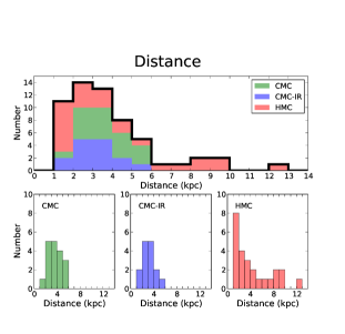
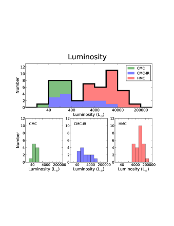
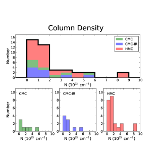
Figure 1: Distribution of kinematic distance, bolometric luminosity, mass, and column density (N) for our targets. All values were taken from the literature (see Table Weak and Compact Radio Emission in Early High-Mass Star Forming Regions: I. VLA Observations for references). In each case the top panels correspond to the distribution of the sum of the corresponding parameter, and the bottom panels show the distribution for each type of clump independently. We use the near distance for 5 sources which have a kinematic distance ambiguity. Values of masses from Beuther et al. (2002a) were scaled following Beuther et al. (2005). For the total sample, nine sources do not have available values for mass and luminosity.

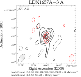
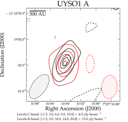
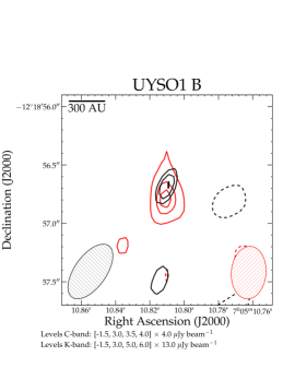
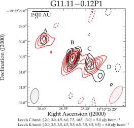
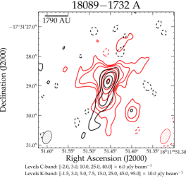
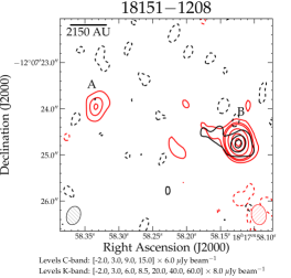
Figure 2: VLA contour plots of the 6 (black) and 1.3 (red) cm combined maps toward all sources associated with mm dust clumps. The synthesized beams are shown in the lower left and right corner for 6 and 1.3 cm, respectively. A scale bar in units of AU is shown in the upper left. We are using the near distance for sources with distance ambiguity. There is not available map at 1.3 cm for 19282$+$1814 A.

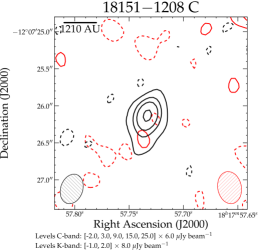
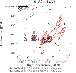
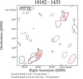
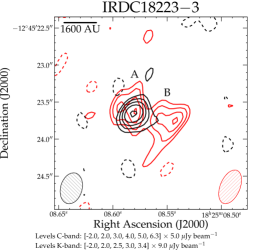
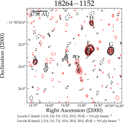
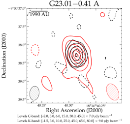
Figure 2: Continued.

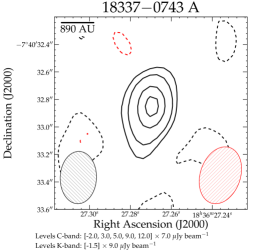
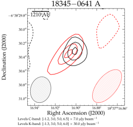
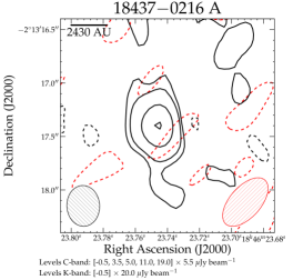
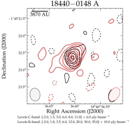
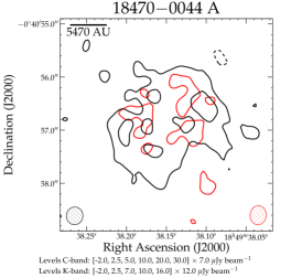
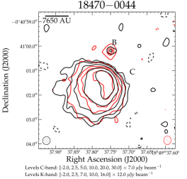
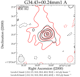
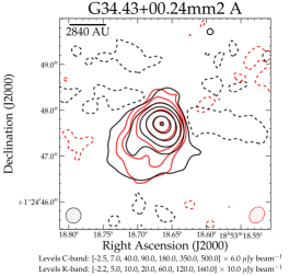
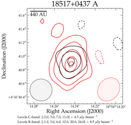
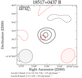
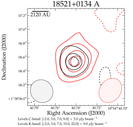
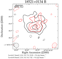
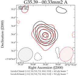
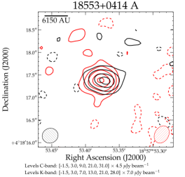
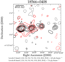
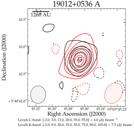
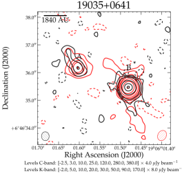
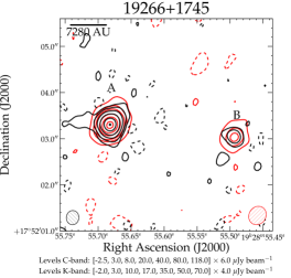
Figure 2: Continued.

Figure 2: Continued.

Figure 2: Continued.

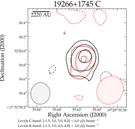
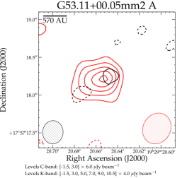
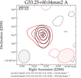
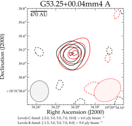
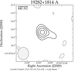
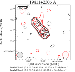
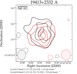
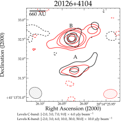
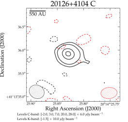
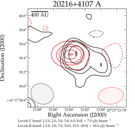
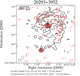
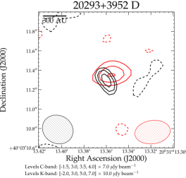
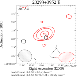
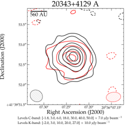
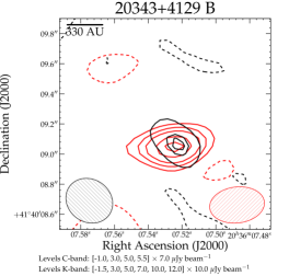
Figure 2: Continued.

Figure 2: Continued.

Figure 2: Continued.

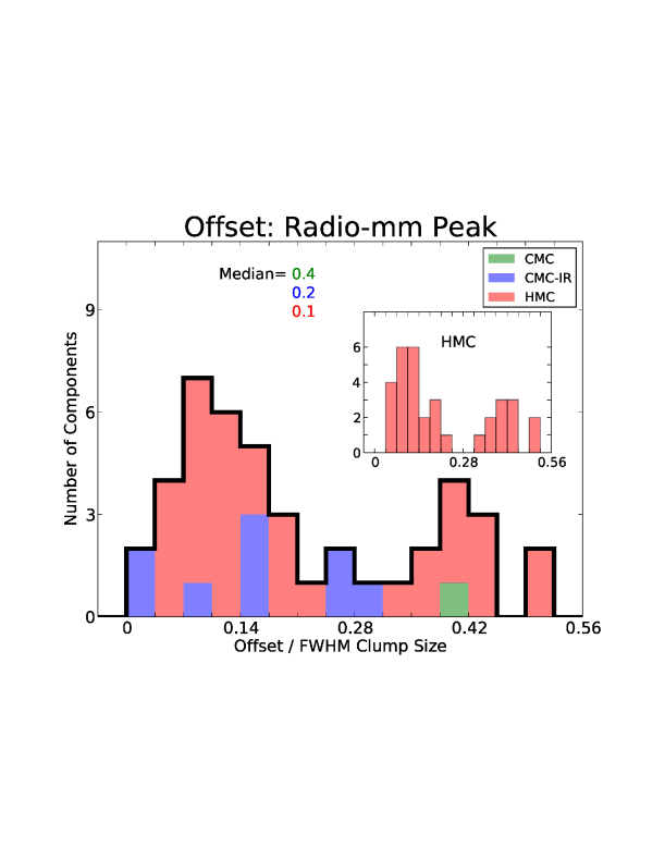
Figure 3: Position offsets between radio sources and the $1.2\,$mm peaks divided by the FWHM size of each clump. The inset shows the distribution only for the HMC detections. If no $1.2\,$mm data was available, we used the median FWHM size for the specific type of clump. The median FWHM sizes for each type of clump in this sample are 31^′′, 25^′′ and 18^′′ for CMCs, CMC–IRs and HMCs, respectively. The average cm positional accuracy is better than 0.1^′′, and the typical positional accuracy for the $1.2\,$mm data is a few arcseconds. Clumps with multiple components (within a radius of 3^′′) have been treated as a single radio source in this histogram. Using a Kolmogorov-Smirnov test to analyze the spatial offset distribution of the HMCs and CMC–IRs we estimated a p-value$=$ 0.34. Thus, there is no strong evidence that these two distributions are different.

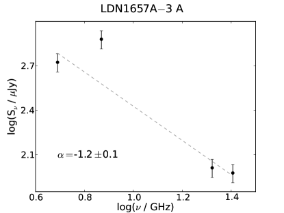
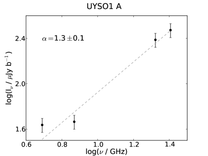
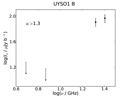
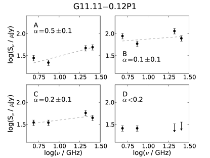
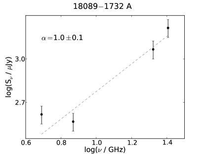
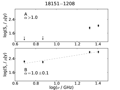
Figure 4: Flux density as a function of frequency for each detected component. Error bars are an assumed uncertainty of 10$\%$ from the flux densities added in quadrature with an assumed 10$\%$ error in calibration. The dashed lines are the best fit to the data from a power law of the form $S_{\nu}$ $\propto$ $\nu^{\alpha}$.

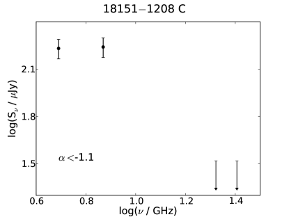
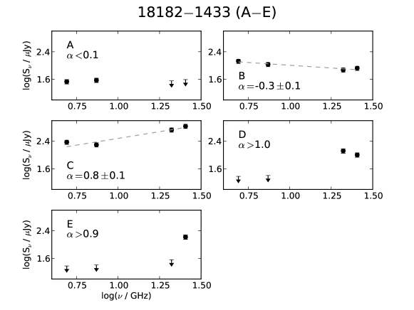
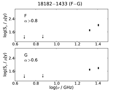
Figure 4: Continued.

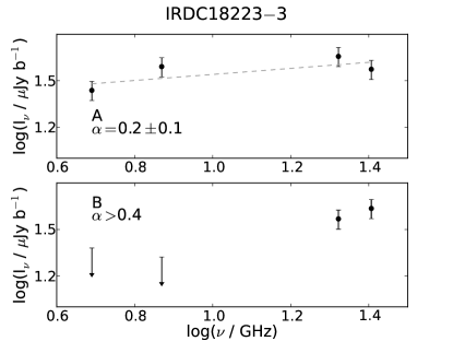
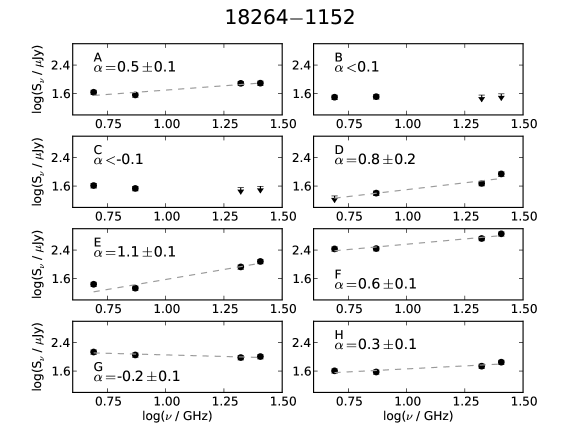
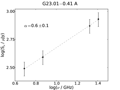
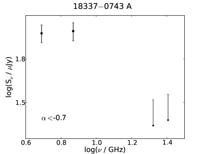
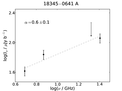
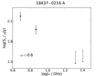
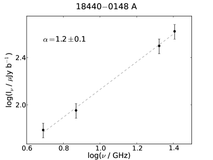
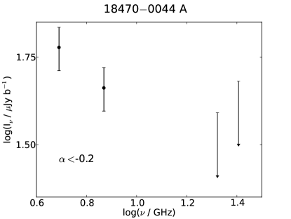
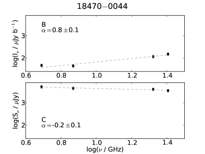
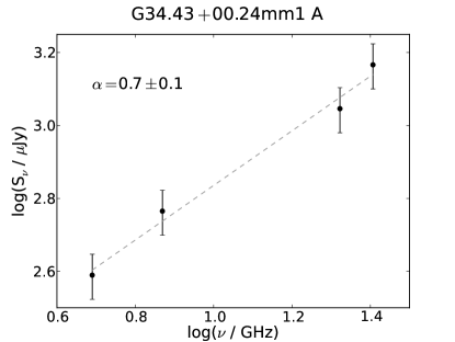
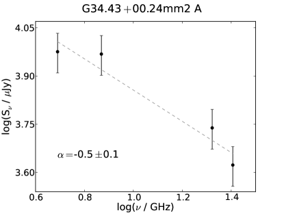
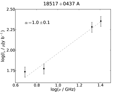
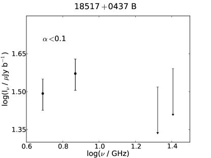
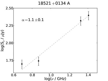
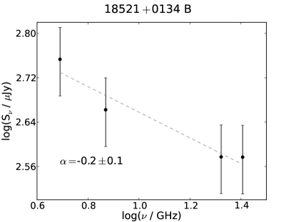
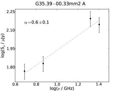
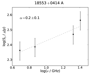
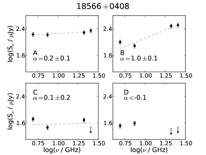
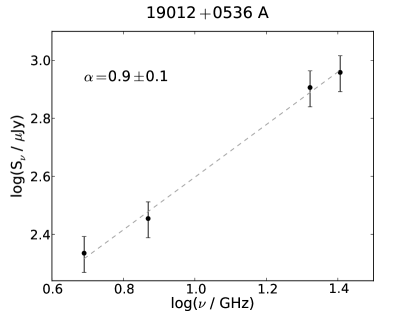
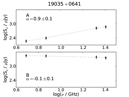
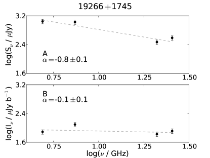
Figure 4: Continued.

Figure 4: Continued.

Figure 4: Continued.

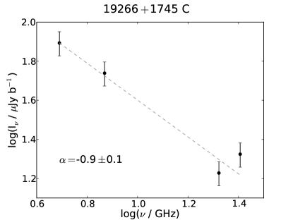
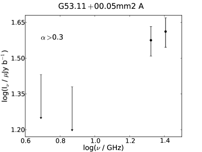
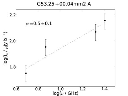
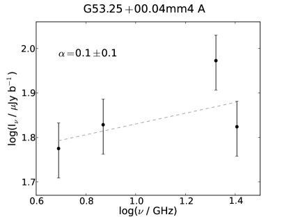
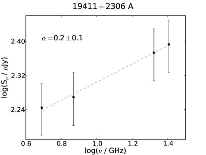
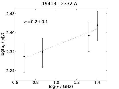
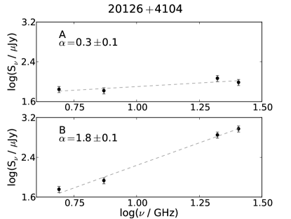
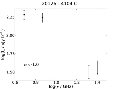
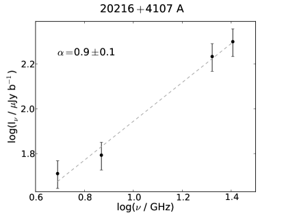
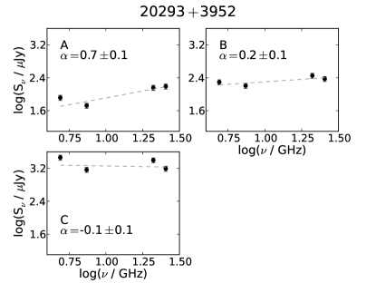
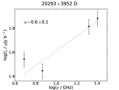
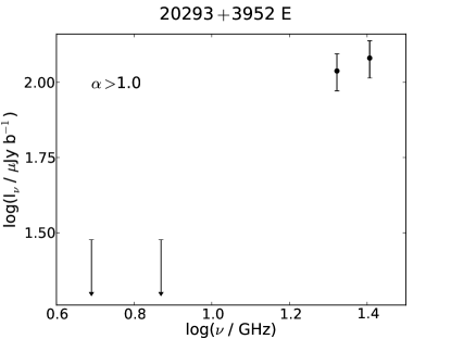
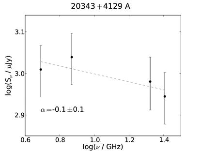
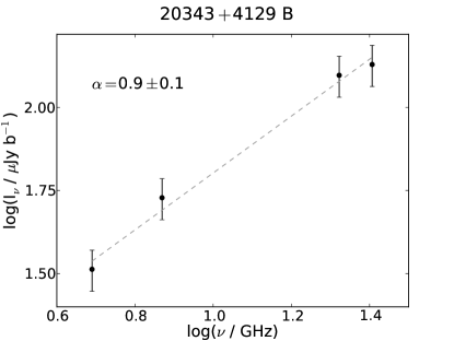
Figure 4: Continued.

Figure 4: Continued.

Figure 4: Continued.

Figure 4: Continued.

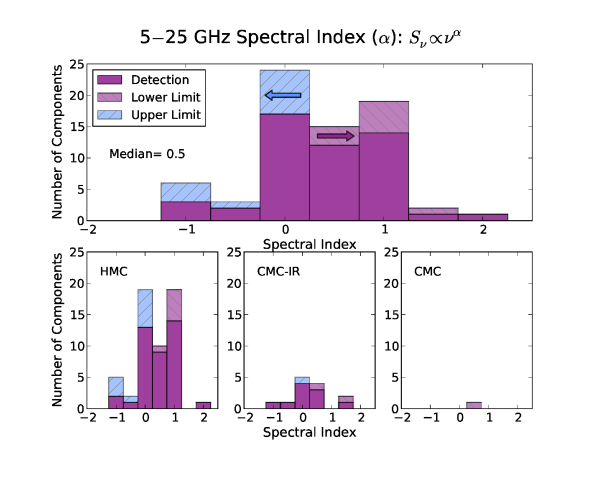
Figure 5: Spectral index ($\alpha$) distribution of 70 radio sources associated with mm–clumps, binned in increments of 0.5 in spectral index. If there is no detection at 6 cm, the estimated value of $\alpha$ is a lower limit, and and if there is no detection at 1.3 cm, the estimated value for $\alpha$ corresponds to an upper limit. The median value refers only to the detections. The distributions at the bottom show the results independently for each type of clump.

References

- AMI Consortium et al. (2011) AMI Consortium, Davies, M. L., Franzen, T. M. O., et al. 2011, MNRAS, 415, 2708
- Anglada et al. (1998) Anglada, G., Villuendas, E., Estalella, R., et al. 1998, AJ, 116, 2953
- Araya et al. (2008) Araya, E. D., Hofner, P., Goss, W. M., et al. 2008, ApJS, 178, 330
- Beuther et al. (2010) Beuther, H., Henning, T., Linz, H., et al. 2010, A&A, 518, L78
- Beuther et al. (2002a) Beuther, H., Schilke, P., Menten, K. M., et al. 2002a, ApJ, 566, 945
- Beuther et al. (2005) —. 2005, ApJ, 633, 535
- Beuther et al. (2002b) Beuther, H., Schilke, P., Sridharan, T. K., et al. 2002b, A&A, 383, 892
- Brunthaler et al. (2009) Brunthaler, A., Reid, M. J., Menten, K. M., et al. 2009, ApJ, 693, 424
- Carrasco-González et al. (2010) Carrasco-González, C., Rodríguez, L. F., Anglada, G., et al. 2010, Science, 330, 1209
- Carrasco-González et al. (2015) Carrasco-González, C., Torrelles, J. M., Cantó, J., et al. 2015, Science, 348, 114
- Cesaroni (2005) Cesaroni, R. 2005, in IAU Symposium, Vol. 227, Massive Star Birth: A Crossroads of Astrophysics, ed. R. Cesaroni, M. Felli, E. Churchwell, & M. Walmsley, 59–69
- Cesaroni et al. (2010) Cesaroni, R., Hofner, P., Araya, E., & Kurtz, S. 2010, A&A, 509, A50
- Cesaroni et al. (1992) Cesaroni, R., Walmsley, C. M., & Churchwell, E. 1992, A&A, 256, 618
- Cesaroni et al. (1991) Cesaroni, R., Walmsley, C. M., Koempe, C., & Churchwell, E. 1991, A&A, 252, 278
- Chambers et al. (2009) Chambers, E. T., Jackson, J. M., Rathborne, J. M., & Simon, R. 2009, ApJS, 181, 360
- Chapin et al. (2008) Chapin, E. L., Ade, P. A. R., Bock, J. J., et al. 2008, ApJ, 681, 428
- Chira et al. (2013) Chira, R.-A., Beuther, H., Linz, H., et al. 2013, A&A, 552, A40
- Ciliegi et al. (2003) Ciliegi, P., Zamorani, G., Hasinger, G., et al. 2003, A&A, 398, 901
- Cyganowski et al. (2008) Cyganowski, C. J., Whitney, B. A., Holden, E., et al. 2008, AJ, 136, 2391
- de Zotti et al. (2005) de Zotti, G., Ricci, R., Mesa, D., et al. 2005, A&A, 431, 893
- Deller et al. (2013) Deller, A. T., Forbrich, J., & Loinard, L. 2013, A&A, 552, A51
- Fazal et al. (2008) Fazal, F. M., Sridharan, T. K., Qiu, K., et al. 2008, ApJ, 688, L41
- Fomalont et al. (1991) Fomalont, E. B., Windhorst, R. A., Kristian, J. A., & Kellerman, K. I. 1991, AJ, 102, 1258
- Forbrich et al. (2004) Forbrich, J., Schreyer, K., Posselt, B., Klein, R., & Henning, T. 2004, ApJ, 602, 843
- Furuya et al. (2008) Furuya, R. S., Cesaroni, R., Takahashi, S., et al. 2008, ApJ, 673, 363
- Garay et al. (1993) Garay, G., Rodriguez, L. F., Moran, J. M., & Churchwell, E. 1993, ApJ, 418, 368
- Gibb & Hoare (2007) Gibb, A. G., & Hoare, M. G. 2007, MNRAS, 380, 246
- Goldsmith et al. (1986) Goldsmith, P. F., Langer, W. D., & Wilson, R. W. 1986, ApJ, 303, L11
- Guzmán et al. (2010) Guzmán, A. E., Garay, G., & Brooks, K. J. 2010, ApJ, 725, 734
- Henning et al. (2010) Henning, T., Linz, H., Krause, O., et al. 2010, A&A, 518, L95
- Hernández-Hernández et al. (2014) Hernández-Hernández, V., Zapata, L., Kurtz, S., & Garay, G. 2014, ApJ, 786, 38
- Kauffmann & Pillai (2010) Kauffmann, J., & Pillai, T. 2010, ApJ, 723, L7
- Keto (2002) Keto, E. 2002, ApJ, 568, 754
- Keto (2003) —. 2003, ApJ, 599, 1196
- Keto (2007) —. 2007, ApJ, 666, 976
- Krumholz & McKee (2008) Krumholz, M. R., & McKee, C. F. 2008, Nature, 451, 1082
- Kurayama et al. (2011) Kurayama, T., Nakagawa, A., Sawada-Satoh, S., et al. 2011, PASJ, 63, 513
- Kurtz et al. (2000) Kurtz, S., Cesaroni, R., Churchwell, E., Hofner, P., & Walmsley, C. M. 2000, Protostars and Planets IV, 299
- Kurtz et al. (1994) Kurtz, S., Churchwell, E., & Wood, D. O. S. 1994, ApJS, 91, 659
- Linz et al. (2010) Linz, H., Krause, O., Beuther, H., et al. 2010, A&A, 518, L123
- López-Sepulcre et al. (2010) López-Sepulcre, A., Cesaroni, R., & Walmsley, C. M. 2010, A&A, 517, A66
- López-Sepulcre et al. (2011) López-Sepulcre, A., Walmsley, C. M., Cesaroni, R., et al. 2011, A&A, 526, L2
- Lu et al. (2014) Lu, X., Zhang, Q., Liu, H. B., Wang, J., & Gu, Q. 2014, ApJ, 790, 84
- Mezger & Henderson (1967) Mezger, P. G., & Henderson, A. P. 1967, ApJ, 147, 471
- Molinari et al. (1996) Molinari, S., Brand, J., Cesaroni, R., & Palla, F. 1996, A&A, 308, 573
- Molinari et al. (2000) —. 2000, A&A, 355, 617
- Molinari et al. (1998) Molinari, S., Brand, J., Cesaroni, R., Palla, F., & Palumbo, G. G. C. 1998, A&A, 336, 339
- Molinari et al. (2008) Molinari, S., Faustini, F., Testi, L., et al. 2008, A&A, 487, 1119
- Moscadelli et al. (2011) Moscadelli, L., Cesaroni, R., Rioja, M. J., Dodson, R., & Reid, M. J. 2011, A&A, 526, A66
- Moscadelli et al. (2013) Moscadelli, L., Cesaroni, R., Sánchez-Monge, Á., et al. 2013, A&A, 558, A145
- Neufeld & Hollenbach (1996) Neufeld, D. A., & Hollenbach, D. J. 1996, ApJ, 471, L45
- Nguyen Luong et al. (2011) Nguyen Luong, Q., Motte, F., Hennemann, M., et al. 2011, A&A, 535, A76
- Olmi et al. (2010) Olmi, L., Araya, E. D., Chapin, E. L., et al. 2010, ApJ, 715, 1132
- Olmi et al. (1993) Olmi, L., Cesaroni, R., & Walmsley, C. M. 1993, A&A, 276, 489
- Peretto et al. (2010) Peretto, N., Fuller, G. A., Plume, R., et al. 2010, A&A, 518, L98
- Pillai et al. (2006a) Pillai, T., Wyrowski, F., Carey, S. J., & Menten, K. M. 2006a, A&A, 450, 569
- Pillai et al. (2006b) Pillai, T., Wyrowski, F., Menten, K. M., & Krügel, E. 2006b, A&A, 447, 929
- Purcell et al. (2008) Purcell, C. R., Hoare, M. G., & Diamond, P. 2008, in Astronomical Society of the Pacific Conference Series, Vol. 387, Massive Star Formation: Observations Confront Theory, ed. H. Beuther, H. Linz, & T. Henning, 389
- Rathborne et al. (2011) Rathborne, J. M., Garay, G., Jackson, J. M., et al. 2011, ApJ, 741, 120
- Rathborne et al. (2010) Rathborne, J. M., Jackson, J. M., Chambers, E. T., et al. 2010, ApJ, 715, 310
- Rathborne et al. (2006) Rathborne, J. M., Jackson, J. M., & Simon, R. 2006, ApJ, 641, 389
- Reid et al. (1995) Reid, M. J., Argon, A. L., Masson, C. R., Menten, K. M., & Moran, J. M. 1995, ApJ, 443, 238
- Reid et al. (2007) Reid, M. J., Menten, K. M., Greenhill, L. J., & Chandler, C. J. 2007, ApJ, 664, 950
- Rodríguez et al. (2012) Rodríguez, L. F., González, R. F., Montes, G., et al. 2012, ApJ, 755, 152
- Rodríguez-Kamenetzky et al. (2016) Rodríguez-Kamenetzky, A., Carrasco-González, C., Araudo, A., et al. 2016, ApJ, 818, 27
- Rosero et al. (2014) Rosero, V., Hofner, P., McCoy, M., et al. 2014, ApJ, 796, 130
- Sakai et al. (2012) Sakai, T., Sakai, N., Furuya, K., et al. 2012, ApJ, 747, 140
- Sánchez-Monge et al. (2013a) Sánchez-Monge, Á., Beltrán, M. T., Cesaroni, R., et al. 2013a, A&A, 550, A21
- Sánchez-Monge et al. (2013b) Sánchez-Monge, Á., Kurtz, S., Palau, A., et al. 2013b, ApJ, 766, 114
- Sánchez-Monge et al. (2011) Sánchez-Monge, Á., Pandian, J. D., & Kurtz, S. 2011, ApJ, 739, L9
- Sánchez-Monge et al. (2013c) Sánchez-Monge, Á., Palau, A., Fontani, F., et al. 2013c, MNRAS, 432, 3288
- Sanhueza et al. (2012) Sanhueza, P., Jackson, J. M., Foster, J. B., et al. 2012, ApJ, 756, 60
- Sanna et al. (2014) Sanna, A., Cesaroni, R., Moscadelli, L., et al. 2014, A&A, 565, A34
- Sato et al. (2014) Sato, M., Wu, Y. W., Immer, K., et al. 2014, ApJ, 793, 72
- Shepherd & Churchwell (1996) Shepherd, D. S., & Churchwell, E. 1996, ApJ, 457, 267
- Smith et al. (2006) Smith, H. A., Hora, J. L., Marengo, M., & Pipher, J. L. 2006, ApJ, 645, 1264
- Sridharan et al. (2002) Sridharan, T. K., Beuther, H., Schilke, P., Menten, K. M., & Wyrowski, F. 2002, ApJ, 566, 931
- Tanaka et al. (2016) Tanaka, K. E. I., Tan, J. C., & Zhang, Y. 2016, ApJ, 818, 52
- Wilson et al. (2003) Wilson, T. L., Boboltz, D. A., Gaume, R. A., & Megeath, S. T. 2003, ApJ, 597, 434
- Wood & Churchwell (1989) Wood, D. O. S., & Churchwell, E. 1989, ApJ, 340, 265
- Wu et al. (2014) Wu, Y. W., Sato, M., Reid, M. J., et al. 2014, A&A, 566, A17
- Xu et al. (2011) Xu, Y., Moscadelli, L., Reid, M. J., et al. 2011, ApJ, 733, 25
- Zhang et al. (2001) Zhang, Q., Hunter, T. R., Brand, J., et al. 2001, ApJ, 552, L167
- Zhang et al. (2007) Zhang, Q., Sridharan, T. K., Hunter, T. R., et al. 2007, A&A, 470, 269
- Zinnecker & Yorke (2007) Zinnecker, H., & Yorke, H. W. 2007, ARA&A, 45, 481