Influence of coherent adiabatic excitation on femtosecond transient signals

Abstract

The transient signals derived from femtosecond pump-probe experiments are analyzed in terms of the coherent evolution of the energy levels perturbed by the excitation pulse. The model system is treated as the sum of independent two-level subsystems that evolve adiabatically or are permanently excited, depending on the detuning from the central wavelength of the excitation laser. This approach will allow us to explain numerically and analytically the convergence between the coherent and incoherent (rate equations) treatments for complex multi-level systems. It will be also shown that the parameter that determines the validity of the incoherent treatment is the distribution of states outside and inside the laser bandwidth, rather than the density of states as it is commonly accepted.

1 Introduction

The substantial evolution of laser sources during the last decades has permitted to monitor, and even control processes taking place in a broad range of time scales. More recently, the efforts in the development of coherent sources of ultrashort pulse duration, i.e., attosecond (as) and femtosecond (fs), together with the increase control over the laser pulses, have provided an ideal tool for recording snapshots of ultrafast evolving systems (see for example DRES02 ; UIBER07 ; ZEW88 ; CAVA07 ; HER96 ; GOR97 ; Skan10 and reference therein). Nowadays, experiments with femtosecond resolution in the fields of Chemistry, Physics and Biology are carried out routinely by using a great variety of pump probe methods, e.g., transient ionization, fluorescence up conversion, fluorescence dip spectroscopy, and femtosecond time resolved Raman ChemRev04 . In these techniques, the system is excited by one (or more) photons of the pump pulse triggering simultaneously in all the particles the process of interest. After a variable temporal delay, the absorption of another (or more) photons from the probe laser produces a measurable signal. The dependence of the system response on the pump probe delay contains the desired information on the dynamics of the process.

Modeling the collected time dependent signals is pivotal for the correct extraction of the information contained in the experimental data. There are two possible approaches for this task: an incoherent treatment based on rate equations, and a coherent model where the interaction of the system with the pump pulse is described by the solution of the time dependent Schrödinger equation (or the equivalent Bloch equations). Let us consider that the system can be described by a two-state model. Three different regimes can be distinguished. If the losses dominates the dynamics of the system, the coherence induced by the laser is lost very rapidly, i.e., we can apply adiabatic elimination Sh90 , and therefore the incoherent treatment provides an accurate description of the dynamics. On the other hand, if the losses are much slower than the pump pulse duration, the incoherent treatment can be applied once again if one is not interested in reproducing the excitation process. Finally, in a situation where the dynamics of interest is of the order of the excitation pulse, the temporal information is given by the solution of the time dependent Schrödinger equation.

However, this simple two-state model is in principle not applicable when the pump laser bandwidth is large enough to couple more than one single state, as it is usually found in molecules, clusters, and solids. In this scenario, a full theoretical treatment requires of very expensive quantum dynamical calculations, and it is usually not accessible, being the ordinary approach to reduce this coherently excited multistate system to an incoherently excited two-state system. The accuracy of this approximation has been tested elsewhere IHER06 , proving to be very effective as long as the determination of the zero delay between pump and probe laser pulses is made correctly.

The aim of the present paper is to explore the applicability of the coherent and incoherent approximation to the modeling of femtosecond transients derived from molecular dynamics. Although the coherent excitation of quasicontinuum systems has been a matter of intense research, and the effect of dephasing and density of states well documented experimentally, and rigorously described theoretically (see for example IHER06 ; MUK95 ; KYR85 and references therein), herein we adopt a different simpler approach from the perspective of the adiabatic evolution of the levels outside the laser bandwidth. This phenomenon is generally known as Coherent Population Return (CPR) Vi01 ; Al06 . In this model a coherently excited multistate system is treated as the sum of independent coherently excited two-state systems with variable detuning from the central wavelength of the excitation laser. This procedure will allow us to justify qualitatively, and analytically with the help of Fourier analysis, the use of the incoherent approximation for such complex systems. We will provide analytical expressions to quantify the error carried out by this treatment, demonstrating that the critical parameter that determines the validity of this approach is the distribution of states with respect to the laser bandwidth, rather than the density of states as it is commonly accepted. Furthermore, this treatment underlines the importance of considering CPR for a correct description of laser-matter interaction Al10 ; Mon10

2 Theoretical models

2.1 Two-state system

For coherent interactions the description of the population dynamics is provided by the time dependent Schrödinger equation

$$i\hbar\frac{\partial\Psi(t)}{\partial t}=H(t)\Psi(t),$$ (1)

where $\Psi(t)$ is the statevector of the system, and $H(t)$ the Hamiltonian including the interaction with a radiation field.

Let us consider a two-state system interacting with the electric field of a laser pulse with carrier frequency $\omega$, detuned from the transition frequency by $\Delta$. This situation is described by Fig 1.

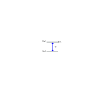
Figure 1: Two-state system interacting with a radiation field. The laser detuning from resonance is represented by $\Delta$. The energies of the excited and ground states are $E_{2}$ and $E_{1}$ respectively.

The time dependent Hamiltonian in the electric dipole approximation can be written as

$$H(t)=H^{0}+H^{I}(t),$$ (2)

where $H^{0}$ is the two-state field free Hamiltonian with energies $E_{1}$ and $E_{2}$

$$H^{0}=\left[\begin{array}[]{cc}E_{1}&0\\ 0&E_{2}\end{array}\right],$$ (3)

and $H^{I}$ is the interacting Hamiltonian

$$H^{I}(t)=\left[\begin{array}[]{cc}0&\langle\psi_{1}|\textrm{V}|\psi_{2}\rangle\\ \langle\psi_{2}|\textrm{V}|\psi_{1}\rangle&0\end{array}\right],$$ (4)

with

$$\textrm{V}=-\textbf{d}\cdot[\textbf{e}\mathcal{E}(t)\cos\omega t],$$ (5)

being d the dipole moment, and e and $\mathcal{E}(t)$ the polarization direction and the slow varying envelope of the electric field respectively.

If as customary the rotating wave approximation (RWA) is applied for neglecting the fast oscillating terms Sh90 , the RWA-Hamiltonian reads

$$H^{RWA}=\frac{\hbar}{2}\left[\begin{array}[]{cc}0&\Omega(t)\\ \Omega(t)&2\Delta\end{array}\right],$$ (6)

where $\Omega(t)$ is the Rabi frequency, i.e., the interaction energy divided by $\hbar$,

$$\Omega(t)=-(\textbf{d}\cdot\textbf{e})\mathcal{E}(t)/\hbar,$$ (7)

and $\Delta$ the laser detuning

$$\Delta=\frac{(E_{2}-E_{1})}{\hbar}-\omega.$$ (8)

It is convenient to describe the population dynamics in the adiabatic basis $\left[\Phi_{+},\Phi_{-}\right]$,which is the basis formed by the instantaneous eigenstates of the Hamiltonian described by Eq. 6. These adiabatic eigenstates can be written as

$$\Phi_{+}(t)=\psi_{1}\sin\vartheta(t)+\psi_{2}\cos\vartheta(t),$$ (9)

$$\Phi_{-}(t)=\psi_{1}\cos\vartheta(t)-\psi_{2}\sin\vartheta(t),$$ (10)

where $\vartheta(t)$ is the mixing angle

$$\vartheta(t)=\frac{1}{2}\arctan\frac{\Omega(t)}{\Delta},$$ (11)

and $\psi_{j}$ ($j=1,2$) are the bare states. The corresponding eigenenergies are

$$\lambda_{\pm}=\frac{1}{2}\left[\Delta\pm\sqrt{\Omega^{2}(t)+\Delta^{2}}\right].$$ (12)

Let us assume $\Omega(t)$ to be negligibly small outside a finite time interval $t_{i}<t<t_{f}$, i.e., outside the pulse duration $\tau=t_{f}-t_{i}$. Consider now the case of the laser frequency detuned from exact resonance, i.e., $\Delta\gtrsim 1/\tau$. If at the beginning of the interaction all the population is in the ground state, the statevector of the system $\Psi(t)$ at time $t=-\infty$ is aligned parallel to the adiabatic state $\Phi_{-}(t)$ because $\Psi(-\infty)=\Phi_{-}(-\infty)=\psi_{1}$. If the evolution of the system is adiabatic, that means the Hamiltonian varies sufficiently slow in time, the statevector of the system $\Psi(t)$ remains always aligned with the adiabatic state $\Phi_{-}(t)$. Thus, during the excitation process when $t_{i}<t<t_{f}$ and $\Omega(t)\neq 0$, the statevector $\Psi(t)$ is a coherent superposition of the bare states (see Eq. 10). Therefore, some population is transiently excited to the upper state. However at the end of the interaction when $t=+\infty$, the statevector of the system becomes once again aligned with the initial state $\psi_{1}$, i.e., $\Psi(+\infty)=\Phi_{-}(+\infty)=\psi_{1}$. The population transferred during the process from the ground state to the excited state returns completely to the ground state after the excitation process. No population resides permanently in the excited state, no matter how large the transient intensity of the laser pulse may be (see Fig. 2). This coherent phenomenon is called Coherent Population Return (CPR) Vi01 ; Al06 . It can be shown Vi01 that the condition for smooth adiabatic evolution – and hence CPR– is just the adiabatic condition $|\Delta|\gtrsim 1/\tau$. It is important to notice that the adiabatic condition is independent of $\Omega(t)$, and therefore of the laser intensity.

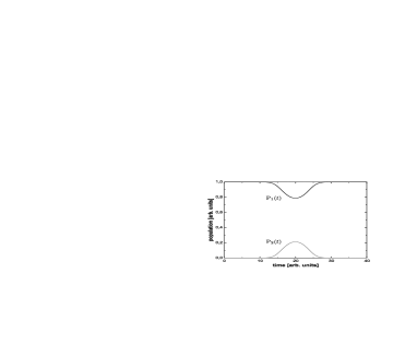
Figure 2: Population dynamics in the case of Coherent Population Return (see Eq. 2.3.2 for the analytical expressions of the populations). P_i is the population of state i (i=1, 2).

It is necessary to consider now a probe process to detect the population transferred to state $\psi_{2}$, e.g., by ionization of the excited state with a short probe laser pulse. According to our previous discussion, if the systems evolves adiabatically ($|\Delta|\gtrsim 1/\tau$) no population remains in the excited state once the pump pulse is over due to CPR, and the ionization signal is produced exclusively when pump and probe pulses overlap in time. On the other hand, if the evolution of the system is diabatic, meaning $|\Delta|\lesssim 1/\tau$, there is a permanent population transferred to the excited state, and consequently, ionization signal when pump and probe pulse do not temporally overlap.

2.2 Extension of the two-state model to multi-state systems

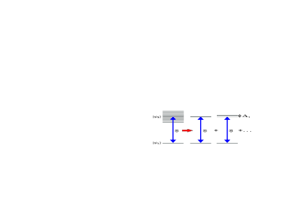
Figure 3: Multistate system as the sum of independent two-state systems with different detunings.

So far, we have assumed a two-state system. However, this simple model can not be usually applied to real systems where inside the laser bandwidth a substantial number of states are excited, being necessary to consider a more general situation. If as a first approximation we neglect any interaction between the excited states, and assume that the losses of the system are much slower than the excitation process, we can model a multistate system by means of the sum of multiple individual two-state systems with different detunings with respect to the excitation laser (see Fig. 3). It is worth to notice that the mechanisms that couple different excited levels as internal vibrational redistribution (IVR) in the case of vibronic levels, take place usually on hundreds of femtoseconds. Thus, for fs laser pulses this approximation is valid.

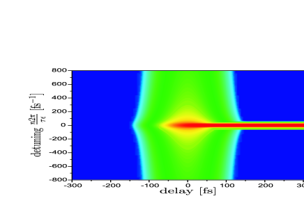
Figure 4: Ionization signal versus detuning and delay between pump and probe laser (1+3’). The parameters chosen for the simulation were: pump pulse duration (full width at half maximum (FWHM) of the peak intensity) $\tau=50$ fs, probe pulse duration $\tau_{Pr}=50$ fs, peak Rabi frequency $\Omega=9.4\,10^{-4}\,\textrm{fs}^{-1}$, peak ionization loss rate $\Gamma=4\,10^{-6}\,\textrm{fs}^{-1}$, number of states per $1/\tau$  $\epsilon=50$.

Figure 4 shows the ionization signal versus detuning of the pump pulse, and temporal delay between pump and probe pulses, for the system proposed in Fig. 1. As we have previously discussed, we can see that only for those detunings that do not fulfilled the adiabatic condition ($|\Delta|\lesssim 1/\tau$), there is a permanent transfer of population to the excited state, and therefore, a transient ionization signal when pump and probe laser pulses do not temporally overlap. According to the model described in Fig. 3, the total ionization signal will be the sum of the ionization signals obtained for different $\Delta$. This is shown in Fig. 5 together with the solution to the time dependent Schrödinger equation on resonance (coherent limit), and the solution of the kinetic model (incoherent limit) for a two-state system. We can see that the coherent excitation of a multistate system, under certain conditions that will be discussed in the next section, is equivalent to the incoherent excitation of a two-state system. This well known result IHER06 simplifies enormously the analysis of pump probe experiments involving a large number of states. Additionally, for the reliable interpretation of the experimental data, it is necessary an exact determination of the zero delay between pump and probe laser pulses. A widely used method to determine the zero delay is to assign it to the position where the excitation signal of a long living state reaches half of its maximum value. Figure 5 shows that this criterion is only valid in the case of the incoherent limit, while for the coherent treatment the 1/2 value is shifted $0.327\tau$ respect to the zero delay position. Therefore, in establishing the zero delay time is necessary to know beforehand what kind of behavior the problem system presents.

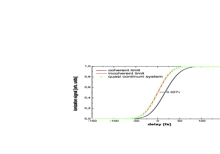
Figure 5: Normalized ionization signal as a function of the delay between pump and probe pulses, for the different possible approaches to the problem: solution of the time dependent Schrödinger equation for a two-state system on resonance (black solid line), solution of rate equations (red solid line), and multiple two-state approximation (green circles). $\tau$ is the pulse duration full width at half maximum (FWHM) of the peak intensity.

2.3 Results and discussion

2.3.1 Qualitative convergence of the coherent and incoherent models

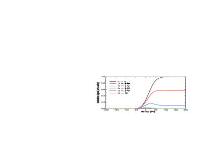
Figure 6: Ionization signal versus delay between pump and probe pulses for different detunings. All the signals are normalized with respect to the maximum signal obtained at $\Delta=0$.

According to our previous discussion, the ionization signal of a quasi continuum system has two different contributions: a step-like transient signal for those detunings that do not fulfilled the adiabatic condition, and a symmetric signal with respect to the delay between pump and probe laser pulses, for those detunings that fulfilled the adiabatic condition (see Fig. 6). When both contributions are added up, the latter is the responsible for the change in the slope that shifts the transient signal to earlier times (see Fig. 5). Since the contributions to the signal coming from the non adiabatic region ($\Delta\lesssim 1/\tau$), is much more intense than the one coming from the adiabatic region ($\Delta\gtrsim 1/\tau$), it is necessary to have a large number of states inside the adiabatic region, i.e., outside the pump laser bandwidth, to reach the convergence to the incoherent limit. If this is not the case, the final situation will be an intermediate case between the coherent and the incoherent limits, being necessary a more elaborated analysis of the experimental results.

2.3.2 Analytical demonstration

The convergence of the incoherent and the coherent treatments can also be demonstrated analytically. Let us define the intensity like

$$\textrm{I}(t)=\textrm{I}_{0}f(t)^{2}=\textrm{I}_{0}e^{-4\textrm{Ln}2\frac{t^{2}}{\tau^{2}}}$$ (13)

where $\textrm{I}_{0}$ is the peak intensity, and $\tau$ the pulse duration (FWHM), the Rabi frequency like

$$\Omega(t)=\Omega_{0}f(t)=\Omega_{0}e^{-2\textrm{Ln}2\frac{t^{2}}{\tau^{2}}}$$ (14)

where $\Omega_{0}$ is the peak Rabi frequency, and let us suppose a two-state system (see Fig. 1). In the case of incoherent excitation, it can be easily shown that the evolution of the population in the target state is described by

$$\textrm{P}_{2}(t)=\frac{1}{2}\left(1-\textrm{exp}\left(-\alpha\int_{-\infty}^{t}\textrm{I}(t^{\prime})\textrm{d}t^{\prime}\right)\right)$$ (15)

where $\alpha$ is the absorption coefficient Sh90 .

Considering a situation where the population of the ground state is barely perturbed, which is a reasonable approximation for fs pulses excitation, the population in the excited state reads:

$$\textrm{P}_{2}(t)=\frac{\alpha}{2}\int_{-\infty}^{t}\textrm{I}(t^{\prime})\textrm{d}t^{\prime}.$$ (16)

For coherent excitation the description of the population evolution is based on the solution of the time dependent Schrödinger equation with an appropriate Hamiltonian. Taking into account the time dependent Hamiltonian in the electric dipole approximation for a two-state system described by Eq. 6, the time dependent Schrödinger equation reads

$$\imath\hbar\frac{\partial}{\partial t}\left(\begin{array}[]{cc}C_{1}(t)\\ C_{2}(t)\end{array}\right)=(\hbar/2)\left[\begin{array}[]{cc}0&\Omega(t)\\ \Omega(t)&2\Delta\end{array}\right]\left(\begin{array}[]{cc}C_{1}(t)\\ C_{2}(t)\end{array}\right),$$ (17)

being $C_{j}(t)$ the probability amplitude of state j (j=1, 2) at time t.
If, as mentioned before, the ground state is barely perturbed, i.e., $C_{1}(t)\simeq 1$, the differential equation that describes the temporal evolution of $C_{2}(t)$ is given by

$$\frac{d}{dt}C_{2}(t)+\imath\Delta C_{2}(t)+(\imath/2)\Omega(t)=0.$$ (18)

Hence, the temporal evolution of $C_{2}(t)$ can be written as

$$C_{2}(t)=-\frac{\imath}{2}e^{-\imath\Delta t}\left(\int_{-\infty}^{t}e^{\imath\Delta t^{\prime}}\Omega(t^{\prime})dt^{\prime}\right),$$ (19)

and the population in the excited state is given by

$$\textrm{P}_{2}(t)=|C_{2}(t)|^{2}=\left[\int_{-\infty}^{t}\frac{\Omega(t^{\prime})}{2}\cos(\Delta t^{\prime})dt^{\prime}\right]^{2}$$

$$+\left[\int_{-\infty}^{t}\frac{\Omega(t^{\prime})}{2}\sin(\Delta t^{\prime})dt^{\prime}\right]^{2}.$$ (20)

Once we have obtained the population evolution for coherent and incoherent excitation, and taking into account the model described by Fig. 3, and the numerical results presented in Fig. 5, we obtain the following equality

$$\frac{\frac{\alpha}{2}\int_{-\infty}^{t}\textrm{I}(t^{\prime})\textrm{d}t^{\prime}}{\frac{\alpha}{2}\int_{-\infty}^{+\infty}\textrm{I}(t^{\prime})\textrm{d}t^{\prime}}=\frac{\sum_{n=-\infty}^{+\infty}\left[\left[\int_{-\infty}^{t}\frac{\Omega(t^{\prime})}{2}\cos(\frac{n2\pi}{\tau\epsilon}t^{\prime})dt^{\prime}\right]^{2}+\left[\int_{-\infty}^{t}\frac{\Omega(t^{\prime})}{2}\sin(\frac{n2\pi}{\tau\epsilon}t^{\prime})dt^{\prime}\right]^{2}\right]}{\sum_{n=-\infty}^{+\infty}\left[\left[\int_{-\infty}^{+\infty}\frac{\Omega(t^{\prime})}{2}\cos(\frac{n2\pi}{\tau\epsilon}t^{\prime})dt^{\prime}\right]^{2}+\left[\int_{-\infty}^{+\infty}\frac{\Omega(t^{\prime})}{2}\sin(\frac{n2\pi}{\tau\epsilon}t^{\prime})dt^{\prime}\right]^{2}\right]},$$ (21)

where we have introduced a normalization factor, and have defined the detuning as $\Delta=\frac{n2\pi}{\tau\epsilon}$, being $n$ an integer that takes into account different states as showed in Fig. 3, and $\epsilon$ the number of states contained in $1/\tau$. It is worth mentioning that the factor $2\pi$ has been included to express $\Delta$ in terms of angular frequency.

With the help of the derived expressions, we can easily justify the factor 0.327$\tau$ that differentiates the temporal evolution of P${}_{2}(t)$ in the coherent and incoherent limits (see Fig. 5). For incoherent excitation is straightforward to check that the value P${}_{2}(t)=\frac{1}{2}$ is obtained at $t=0$. In the case of coherent excitation we have,

$$\frac{\left[\int_{-\infty}^{t}\frac{\Omega(t^{\prime})}{2}dt^{\prime}\right]^{2}}{\left[\int_{-\infty}^{+\infty}\frac{\Omega(t^{\prime})}{2}dt^{\prime}\right]^{2}}=\frac{1}{2}.$$ (22)

Substituting Eq. 14 into Eq. 22 we obtain

$$\frac{1}{2}\left(1+\textrm{Erf}\left[\frac{t\sqrt{2\ln 2}}{\tau}\right]\right)=\frac{\sqrt{2}}{2}.$$ (23)

where Erf is the error function

$$\textrm{Erf}(x)=\frac{2}{\sqrt{\pi}}\int_{0}^{x}e^{-z^{2}}dz.$$ (24)

From Eq. 23

$$\textrm{Erf}\left[\frac{t\sqrt{2\ln 2}}{\tau}\right]=\sqrt{2}-1,$$ (25)

and therefore

$$\frac{t\sqrt{2\ln 2}}{\tau}=0.385,$$ (26)

obtaining finally

$$t=\frac{0.385\,\tau}{\sqrt{2\ln 2}}\simeq 0.327\,\tau.$$ (27)

In the next section we will apply Fourier analysis concepts to derive an analytical justification of Eq. 21.

2.3.3 Fourier analysis

Let us consider a periodic function $f(t)$ with period $a$ and its Fourier series expansion

$$S_{N}=\frac{1}{2}A_{0}+\sum_{n=1}^{N}\left[A_{n}\cos\left(\frac{n\pi t}{a}\right)+B_{n}\sin\left(\frac{n\pi t}{a}\right)\right]$$ (28)

where the coefficients $A_{0}$,$A_{n}$, and $B_{n}$ are

$$A_{0}=\frac{1}{a}\int_{-a}^{a}f(t)dt$$

$$A_{n}=\frac{1}{a}\int_{-a}^{a}f(t)\cos\left(\frac{n\pi t}{a}\right)dt$$

$$B_{n}=\frac{1}{a}\int_{-a}^{a}f(t)\sin\left(\frac{n\pi t}{a}\right)dt.$$ (29)

Thus we have

$$f(t)\sim S_{N}.$$ (30)

It can be shown Walker88 that

$$\int_{-a}^{a}\left(f(t)-S_{N}\right)^{2}dt=$$

$$\left(\frac{1}{a}\int_{-a}^{a}f(t)^{2}dt-\left(\frac{1}{2}A_{0}^{2}+\sum_{n=1}^{N}\left(A_{n}^{2}+B_{n}^{2}\right)\right)\right).$$ (31)

If we let $N$ tend to infinity, the convergence of the Fourier series $S_{N}$ to $f(t)$ implies that the left side in Eq. 2.3.3 is equal to zero, and therefore we obtain

$$\frac{1}{a}\int_{-a}^{a}f(t)^{2}dt=\frac{1}{2}A_{0}^{2}+\sum_{n=1}^{\infty}\left(A_{n}^{2}+B_{n}^{2}\right),$$ (32)

that is known as the Parseval’s equality.

Let us define now the following coefficients:

$$A_{0t}=\frac{1}{a}\int_{-a}^{t}f(t^{\prime})dt^{\prime}$$

$$A_{nt}=\frac{1}{a}\int_{-a}^{t}f(t^{\prime})\cos\left(\frac{n\pi t^{\prime}}{a}\right)dt^{\prime}$$

$$B_{nt}=\frac{1}{a}\int_{-a}^{t}f(t^{\prime})\sin\left(\frac{n\pi t^{\prime}}{a}\right)dt^{\prime}.$$ (33)

Substituting the above coefficient in the Parseval’s equality we can write

$$\frac{\frac{1}{a}\int_{-a}^{t}f(t^{\prime})^{2}dt^{\prime}+\frac{1}{a}\int_{t}^{a}f(t^{\prime})^{2}dt^{\prime}}{\frac{1}{a}\int_{-a}^{a}f(t)^{2}dt}=$$

$$\frac{\frac{1}{2}\left(A_{0t}+\left(A_{0}-A_{0t}\right)\right)^{2}}{\frac{1}{2}A_{0}^{2}+\sum_{n=1}^{\infty}\left(A_{n}^{2}+B_{n}^{2}\right)}+$$

$$\frac{\sum_{n=1}^{\infty}\left(\left(A_{nt}+\left(A_{n}-A_{nt}\right)\right)^{2}+\left(B_{nt}+\left(B_{n}-B_{nt}\right)\right)^{2}\right)}{\frac{1}{2}A_{0}^{2}+\sum_{n=1}^{\infty}\left(A_{n}^{2}+B_{n}^{2}\right)}.$$ (34)

Rearranging we obtain the following expression

$$\frac{\frac{1}{a}\int_{-a}^{t}f(t^{\prime})^{2}dt^{\prime}}{\frac{1}{a}\int_{-a}^{a}f(t)^{2}dt}=\frac{\frac{1}{2}A_{0t}^{2}+\sum_{n=1}^{\infty}\left(A_{nt}^{2}+B_{nt}^{2}\right)}{\frac{1}{2}A_{0}^{2}+\sum_{n=1}^{\infty}\left(A_{n}^{2}+B_{n}^{2}\right)}+\xi.$$ (35)

where

$$\xi=-\frac{\frac{1}{a}\int_{t}^{a}f(t^{\prime})^{2}dt^{\prime}}{\frac{1}{a}\int_{-a}^{a}f(t)^{2}dt}+$$

$$\frac{\frac{1}{2}\left(A_{0}^{2}-A_{0t}^{2}\right)+\sum_{n=1}^{\infty}\left(\left(A_{n}^{2}-A_{nt}^{2}\right)+\left(B_{n}^{2}-B_{nt}^{2}\right)\right)}{\frac{1}{2}A_{0}^{2}+\sum_{n=1}^{\infty}\left(A_{n}^{2}+B_{n}^{2}\right)}.$$ (36)

The term $\xi$ takes into account the error produced in Eq. 32 for not extending the integral limits to the period $a$. Obviously if we set $t=a$ we obtain $\xi=0$.

If we define now

$$\Omega(t)=\Omega_{0}e^{-2Ln2\frac{t^{2}}{\tau^{2}}}=\Omega_{0}f(t),$$ (37)

$$I(t)=I_{0}e^{-4Ln2\frac{t^{2}}{\tau^{2}}}=I_{0}f(t)^{2},$$ (38)

$$\Delta=\frac{2\pi}{\tau\epsilon},$$ (39)

where $\epsilon$ is the number of states contained in $1/\tau$,

$$a=\frac{\tau\epsilon}{2}.$$ (40)

Introducing these definitions in Eq. 35, we finally obtain

$$\frac{\frac{\alpha}{2}\int_{-\tau\epsilon/2}^{t}\textrm{I}(t^{\prime})\textrm{d}t^{\prime}}{\frac{\alpha}{2}\int_{-\tau\epsilon/2}^{+\tau\epsilon/2}\textrm{I}(t^{\prime})\textrm{d}t^{\prime}}=\frac{\sum_{n=-\infty}^{+\infty}\left[\left[\int_{-\tau\epsilon/2}^{t}\frac{\Omega(t^{\prime})}{2}\cos(n\frac{2\pi}{\tau\epsilon}t^{\prime})dt^{\prime}\right]^{2}+\left[\int_{-\tau\epsilon/2}^{t}\frac{\Omega(t^{\prime})}{2}\sin(n\frac{2\pi}{\tau\epsilon}t^{\prime})dt^{\prime}\right]^{2}\right]}{\sum_{n=-\infty}^{+\infty}\left[\left[\int_{-\tau\epsilon/2}^{+\tau\epsilon/2}\frac{\Omega(t^{\prime})}{2}\cos(n\frac{2\pi}{\tau\epsilon}t^{\prime})dt^{\prime}\right]^{2}+\left[\int_{-\tau\epsilon/2}^{+\tau\epsilon/2}\frac{\Omega(t^{\prime})}{2}\sin(n\frac{2\pi}{\tau\epsilon}t^{\prime})dt^{\prime}\right]^{2}\right]}+\xi.$$ (41)

Equation 41 is the same that Eq. 21 except for the error term $\xi$. This term tends rapidly to zero when the sum is extended to a large number of states, and we can write Eq. 42.

$$\frac{\frac{\alpha}{2}\int_{-\tau\epsilon/2}^{t}\textrm{I}(t^{\prime})\textrm{d}t^{\prime}}{\frac{\alpha}{2}\int_{-\tau\epsilon/2}^{+\tau\epsilon/2}\textrm{I}(t^{\prime})\textrm{d}t^{\prime}}\simeq\\ \frac{\sum_{n=-\infty}^{+\infty}\left[\left[\int_{-\tau\epsilon/2}^{t}\frac{\Omega(t^{\prime})}{2}\cos(n\frac{2\pi}{\tau\epsilon}t^{\prime})dt^{\prime}\right]^{2}+\left[\int_{-\tau\epsilon/2}^{t}\frac{\Omega(t^{\prime})}{2}\sin(n\frac{2\pi}{\tau\epsilon}t^{\prime})dt^{\prime}\right]^{2}\right]}{\sum_{n=-\infty}^{+\infty}\left[\left[\int_{-\tau\epsilon/2}^{+\tau\epsilon/2}\frac{\Omega(t^{\prime})}{2}\cos(n\frac{2\pi}{\tau\epsilon}t^{\prime})dt^{\prime}\right]^{2}+\left[\int_{-\tau\epsilon/2}^{+\tau\epsilon/2}\frac{\Omega(t^{\prime})}{2}\sin(n\frac{2\pi}{\tau\epsilon}t^{\prime})dt^{\prime}\right]^{2}\right]}.$$ (42)

It is important to point out that in case we do not consider a large number of states, i.e., $N$ does not tend to infinity, the left side in Eq. 2.3.3 is not zero. Thus in this situation, the error term $\xi$ does not only accounts for the error for not extending the integral in Eq. 35 to the full period, but also the for error produced because $S_{N}$ does not exactly converge to $f(t)$.

It is instructive to analyze the behavior of the error term $\xi$ as a function of the number of states contained in the laser bandwidth $\epsilon$. If we choose an arbitrary point, e.g., $t=0$, and taking into account that $\int_{0}^{a}f(t)^{2}dt=\int_{-a}^{a}f(t)^{2}dt/2$, $A_{nt}=A_{n}/2$, and $B_{n}=0$, Eq. 2.3.3 can be written as

$$\xi=\frac{1}{4}-\frac{\sum_{n=1}^{N}B_{nt}^{2}}{\frac{1}{2}A_{0}^{2}+\sum_{n=1}^{N}A_{n}^{2}}.$$ (43)

Figure 7 shows the error term $\xi$ as a function of N for different values of $\epsilon$. We can see that $\xi$ tends to zero more rapidly for small values of $\epsilon$. In other words, if the number of states inside the bandwidth is small, less states outside the bandwidth have to be summed up to reach the incoherent limit.

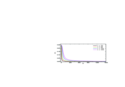
Figure 7: Error term $\xi$ as a function of N, for a different number of states contained in the bandwidth of the pump laser $\epsilon$ ($\tau=50\,\textrm{fs}$).

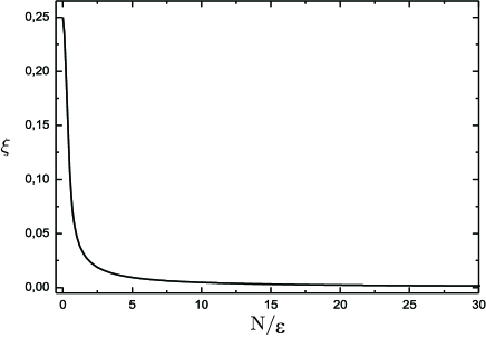
Figure 8: Error term $\xi$ as a function of N/$\epsilon$.

For a better comparison Fig. 8 shows $\xi$ as a function of $N/\epsilon$, i.e., as a function of the number of bandwidths consider in the summations. It is remarkable that for all the different $\epsilon$ the error function takes the same value. In other words, if one maintains constant the ratio between the number of states inside and outside the laser bandwidth the error function is independent of $\epsilon$. This result, as first sight non intuitive, was already sketched in Section 2.3.1 in terms of CPR. If we consider a situation where inside the bandwidth there are many states, large $\epsilon$, a large number of states lying outside the laser bandwidth will be necessary to produce the temporal shift that yields $\xi=0$ (see Fig. 5). According to this analysis, we can conclude that it is not necessary to have a large density of states for ensuring the validity of the incoherent approximation, but just an adequate balance between the states inside and outside the pump laser bandwidth.

3 Conclusions

In conclusion, in the light of concepts of coherent interactions we have demonstrated the suitability of the kinetic model to extract the correct information from pump probe experiments in multistate systems. The validity of the kinetic model applied to such complex systems, has been rationalized in terms of the ratio of states inside and outside the laser bandwidth, showing that if this parameter is kept constant the accuracy of the kinetic model is independent of the density of states. We believe that the field of coherent laser matter interactions applied to problems where historically the coherent nature of light has been sometimes ignored, still offers a large potential for future explorations. We should emphasize the latter results in a scenario where the constant development of shorter pulses KRA09 , i.e., larger bandwidths, and the increasing interest for the ultrafast dynamics of bigger molecules OST09 , i.e., with a large density of states, demand a correct interpretation of laser-matter interaction.

4 Acknowledgments

The authors thank D. Ruano for the most valuable discussions. They also thank the Basque Government (BG) funding through a Complementary Action and the UPV-EHU Consolidated Group Program. Technical and human support provided by the SGIker (UPV/EHU, MICINN, GV/EJ, ESF) is also gratefully acknowledged.

References

- (1) M. Drescher, M. Hentschel, R. Kienberger, M. Uiberacker, V. Yakovlev, A. Scrinzi, Th. Westerwalbesloh, U. Kleineberg, U. Heinzmann, and F. Krausz, Nature 419, 803, 2002.
- (2) M. Uiberacker, T. Uphues, M. Schultze, A. J. Verhoef, V. Yakovlev, M. F. Kling, J. Rauschenberger, N. M. Kabachnik, H. Schroder, M. Lezius, K. L. Kompa, H. G. Muller, M. J. J. Vrakking, S. Hendel, U. Kleineberg, U. Heinzmann, M. Drescher and F. Krausz, Nature 446, 627, 2007.
- (3) A. H. Zewail, Science 242, 1645, 1988.
- (4) A. L. Cavalieri, N. Mller, T. Uphues, V. S. Yakovlev, A. Baltuska, B. Horvath, B. Schmidt, L. Blmel, R. Holzwarth, S. Hendel, M. Drescher, U. Kleineberg, P. M. Echenique, R. Kienberger, F. Krausz and U. Heinzmann, Nature 449, 1029, 2007.
- (5) T. Hertel, E. Knoesel, M. Wolf and G. Ertl, Phys. Rev. Lett. 76, 535, 1996.
- (6) R.J. Gordon, and S.A. Rice, Ann. Rev. Phys. Chem. 48, 601, 1997.
- (7) E. Skantzakis, P. Tzallas, J. E. Kruse, C. Kalpouzos, O. Faucher, G. D. Tsakiris, and D. Charalambidis, Phys. Rev. Lett. 105, 043902, 2010.
- (8) Femtochemistry, Chem. Rev. 104, 4, 1717-2124, 2004.
- (9) B. W. Shore, The Theory of Coherent Atomic Excitation, Wiley, NY, 1990.
- (10) I. V. Hertel, and W. Radloff, Rep. Prog. Phys. 69, 1897 2006.
- (11) S. Mukamel, Nonlinear Optical Spectroscopy, Oxford University Press, 1995.
- (12) E. Kyrölä, and J. H. Eberly, J. Chem. Phys., 82(4), 1985.
- (13) N. V. Vitanov, B. W. Shore, L. Yatsenko, K. Bhmer, T. Halfmann, T. Rickes, and K. Bergmann, Opt. Commun., 199, 117126, 2001.
- (14) A. Peralta Conde, L. Brandt, and T. Halfmann, Phys. Rev. Lett. 97, 243004, 2006.
- (15) A. Peralta Conde, R. Montero, A.Longarte, and F. Castano, Phys. Chem. Chem. Phys. 12, 47, 15501-15504, 2010.
- (16) R. Montero, A. Peralta Conde, A. Longarte, and F. Castano, ChemPhysChem 11, 16, 34203423, 2010.
- (17) J. S. Walker, Fourier analysis, Oxford University press, 1988.
- (18) F. Krausz, and M. Ivanov, Rev. Mod. Phys., 81, 163, 2009.
- (19) E. Ostroumov, M. G. Müller, C. M. Marian, M. Kleinschmidt, and A. R. Holzwarth, Phys. Rev. Lett. 103, 108302, 2009.