Low-Rank Tensor Decomposition-Aided Channel Estimation for Millimeter Wave MIMO-OFDM Systems

Abstract

We consider the problem of downlink channel estimation for millimeter wave (mmWave) MIMO-OFDM systems, where both the base station (BS) and the mobile station (MS) employ large antenna arrays for directional precoding/beamforming. Hybrid analog and digital beamforming structures are employed in order to offer a compromise between hardware complexity and system performance. Different from most existing studies that are concerned with narrowband channels, we consider estimation of wideband mmWave channels with frequency selectivity, which is more appropriate for mmWave MIMO-OFDM systems. By exploiting the sparse scattering nature of mmWave channels, we propose a CANDECOMP/PARAFAC (CP) decomposition-based method for channel parameter estimation (including angles of arrival/departure, time delays, and fading coefficients). In our proposed method, the received signal at the BS is expressed as a third-order tensor. We show that the tensor has the form of a low-rank CP decomposition, and the channel parameters can be estimated from the associated factor matrices. Our analysis reveals that the uniqueness of the CP decomposition can be guaranteed even when the size of the tensor is small. Hence the proposed method has the potential to achieve substantial training overhead reduction. We also develop Cramér-Rao bound (CRB) results for channel parameters, and compare our proposed method with a compressed sensing-based method. Simulation results show that the proposed method attains mean square errors that are very close to their associated CRBs, and presents a clear advantage over the compressed sensing-based method in terms of both estimation accuracy and computational complexity.

I Introduction

Millimeter-wave (mmWave) communication is a promising technology for future cellular networks [1, 2]. The large bandwidth available in mmWave bands can offer gigabit-per-second communication data rates. However, high signal attenuation at such high frequency presents a major challenge for system design [3]. To compensate for the significant path loss, large antenna arrays should be used at both the base station (BS) and the mobile station (MS) to provide sufficient beamforming gain for mmWave communications [4]. This requires accurate channel estimation which is essential for the proper operation of directional precoding/beamforming in mmWave systems.

Channel estimation in mmWave systems is challenging due to hybrid precoding structures and the large number of antennas. A primary challenge is that hybrid precoding structures [5, 6, 7, 8] employed in mmWave systems prevent the digital baseband from directly accessing the entire channel dimension. This is also referred to as the channel subspace sampling limitation [9, 10], which makes it difficult to acquire useful channel state information (CSI) during a practical channel coherence time. To address this issue, fast beam scanning and searching techniques have been extensively studied, e.g. [9, 11, 12]. The objective of beam scanning is to search for the best beamformer-combiner pair by letting the transmitter and receiver scan the adaptive sounding beams or coded beams chosen from pre-determined sounding beam codebooks. Nevertheless, as the number of antennas increases, the size of the codebook should be enlarged accordingly, which in turn results in an increase in the sounding/training overhead.

Unlike beam scanning techniques whose objective is to find the best beam pair, another approach is to directly estimate the mmWave channel or its associated parameters, e.g. [13, 14, 15, 10, 16]. In particular, by exploiting the sparse scattering nature of the mmWave channels, mmWave channel estimation can be formulated as a sparse signal recovery problem, and it has been shown [13, 14] that substantial reduction in training overhead can be achieved via compressed sensing methods. In [14], an adaptive compressed sensing method was developed for mmWave channel estimation based on a hierarchical multi-resolution beamforming codebook. Compared to the standard compressed sensing method, the adaptive method is more efficient as the training precoding is adaptively adjusted according to the outputs of earlier stages. Nevertheless, this improved efficiency comes at the expense of requiring feedback from the MS to the BS. Other compressed sensing-based mmWave channel estimation methods include [17, 18, 19, 20]. Most of the above existing methods are concerned with estimation of narrowband channels. MmWave systems, however, are very likely to operate on wideband channels with frequency selectivity [21]. In [22], the authors considered the problem of multi-user uplink channel estimation in mmWave MIMO-OFDM systems and proposed a distributed compressed sensing-based scheme by exploiting the angular domain structured sparsity of mmWave wideband frequency-selective fading channels. Precoding design, with limited feedback for frequency selective wideband mmWave channels, was studied in [21].

In this paper, we study the problem of downlink channel estimation for mmWave MIMO-OFDM systems, where wideband frequency-selective fading channels are considered. We propose a CANDECOMP/PARAFAC (CP) decomposition-based method for downlink channel estimation. The proposed method is based on the following three key observations. First, by adopting a simple setup at the transmitter, the received signal at the BS can be organized into a third-order tensor which admits a CP decomposition. Second, due to the sparse scattering nature of mmWave channels, the tensor has an intrinsic low CP rank that guarantees the uniqueness of the CP decomposition. Third, the channel parameters, including angles of arrival/departure, time delays, and fading coefficients, can be easily extracted based on the decomposed factor matrices. We conduct a rigorous analysis on the uniqueness of the CP decomposition. Analyses show that the uniqueness of the CP decomposition can be guaranteed even when the size of the tensor is small. This result implies that our proposed method can achieve a substantial training overhead reduction. The Cramér-Rao bound (CRB) results for channel parameters are also developed, which provides a benchmark for the performance of our proposed method, and also describes the best asymptotically achievable performance. Our experiments show that the mean square errors attained by the proposed method are close to their corresponding CRBs.

Our proposed CP decomposition-based method enjoys the following advantages as compared with the compressed sensing-based method. Firstly, unlike compressed sensing techniques which require to discretize the continuous parameter space into a finite set of grid points, our proposed method is essentially a gridless approach and therefore is free of the grid discretization errors. Secondly, the proposed method captures the intrinsic multi-dimensional structure of the multiway data, which helps achieve a performance improvement. Thirdly, the use of tensors for data representation and processing leads to a very low computational complexity, whereas most compressed sensing methods are usually plagued by high computational complexity. Our simulation results show that our proposed method has a computational complexity as low as the simplest compressed sensing method, i.e. the orthogonal matching pursuit (OMP) method [23], while achieving a much higher estimation accuracy than the OMP. Lastly, the conditions for the uniqueness of the CP decomposition are easy to analyze, and can be employed to determine the exact amount of training overhead required for unique decomposition. In contrast, it is usually difficult to analyze and check the exact recovery condition for generic dictionaries for compressed sensing techniques.

The rest of the paper is organized as follows. In Section II, we provide notations and basics on the CP decomposition. The system model and the channel estimation problem are discussed in Section III. In Section IV, we propose a CP decomposition-based method for mmWave channel estimation. The uniqueness of the CP decomposition is also analyzed. Section V develops CRB results for the estimation of channel parameters. A compressed sensing-based channel estimation method is discussed in Section VI. Computational complexity of the proposed method and the compressed sensing-based method is analyzed in Section VII. Simulation results are provided in Section VIII, followed by concluding remarks in Section IX.

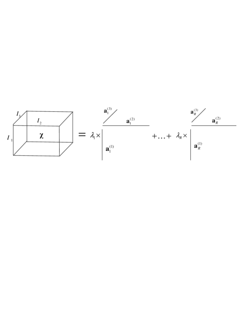
Figure 1: Schematic of CP decomposition.

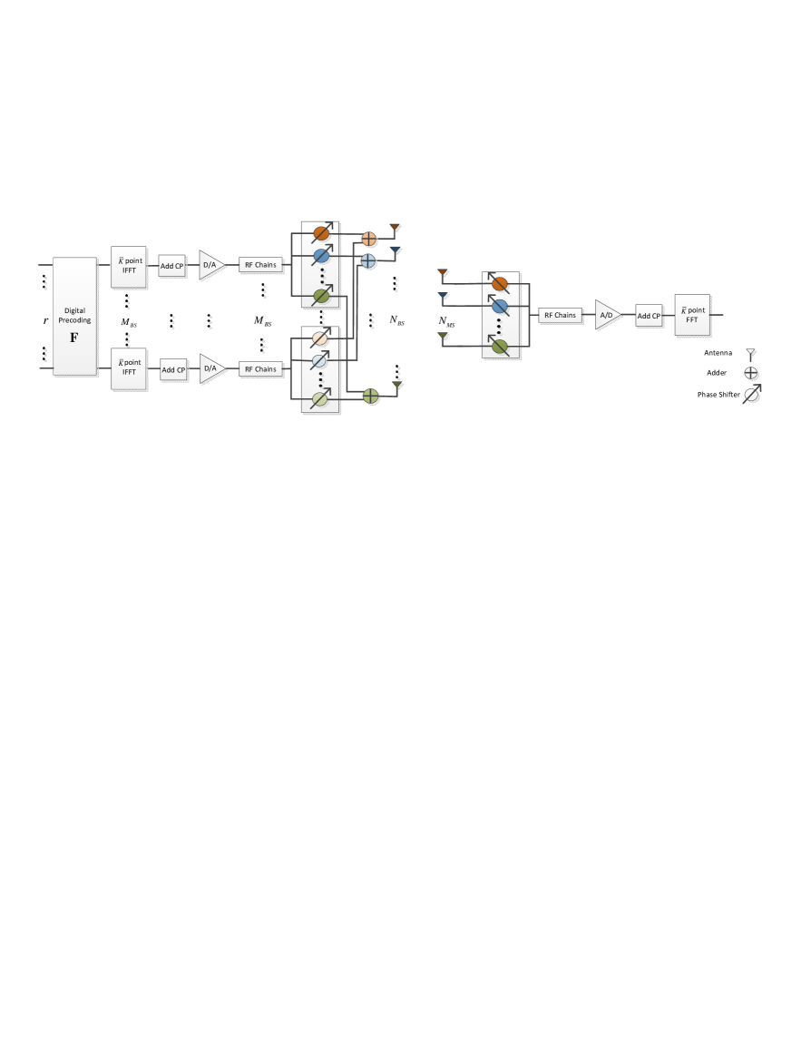
Figure 2: A block diagram of the MIMO-OFDM transceiver that employs hybrid analog/digital precoding.

II Preliminaries

To make the paper self-contained, we provide a brief review on tensors and the CP decomposition. More details regarding the notations and basics on tensors can be found in [24, 25, 26]. Simply speaking, a tensor is a generalization of a matrix to higher-order dimensions, also known as ways or modes. Vectors and matrices can be viewed as special cases of tensors with one and two modes, respectively. Throughout this paper, we use symbols $\otimes$ , $\circ$ , and $\odot$ to denote the Kronecker, outer, and Khatri-Rao product, respectively.

Let $\boldsymbol{\mathcal{X}}\in\mathbb{C}^{I_{1}\times I_{2}\times\cdots\times I_{N}}$ denote an $N$th-order tensor with its $(i_{1},\ldots,i_{N})$th entry denoted by $\mathcal{X}_{i_{1}\cdots i_{N}}$. Here the order $N$ of a tensor is the number of dimensions. Fibers are a higher-order analogue of matrix rows and columns. The mode-$n$ fibers of $\boldsymbol{\mathcal{X}}$ are $I_{n}$-dimensional vectors obtained by fixing every index but $i_{n}$. Slices are two-dimensional sections of a tensor, defined by fixing all but two indices. Unfolding or matricization is an operation that turns a tensor into a matrix. The mode-$n$ unfolding of a tensor $\boldsymbol{\mathcal{X}}$, denoted as $\boldsymbol{X}_{(n)}$, arranges the mode-$n$ fibers to be the columns of the resulting matrix. The CP decomposition decomposes a tensor into a sum of rank-one component tensors (see Fig. 1), i.e.

$$\boldsymbol{\mathcal{X}}=\sum\limits_{r=1}^{R}\lambda_{r}\boldsymbol{a}_{r}^{(1)}\circ\boldsymbol{a}_{r}^{(2)}\circ\cdots\circ\boldsymbol{a}_{r}^{(N)}$$ (1)

where $\boldsymbol{a}_{r}^{(n)}\in\mathbb{C}^{I_{n}}$, the minimum achievable $R$ is referred to as the rank of the tensor, and $\boldsymbol{A}^{(n)}\triangleq[\boldsymbol{a}_{1}^{(n)}\phantom{0}\ldots\phantom{0}\boldsymbol{a}_{R}^{(n)}]\in\mathbb{C}^{I_{n}\times R}$ denotes the factor matrix along the $n$-th mode. Elementwise, we have

$$\mathcal{X}_{i_{1}i_{2}\cdots i_{N}}=\sum\limits_{r=1}^{R}\lambda_{r}a_{i_{1}r}^{(1)}a_{i_{2}r}^{(2)}\cdots a_{i_{N}r}^{(N)}$$ (2)

The mode-$n$ unfolding of $\boldsymbol{\mathcal{X}}$ can be expressed as

$$\boldsymbol{X}_{(n)}=\boldsymbol{A}^{(n)}\boldsymbol{\Lambda}\left(\boldsymbol{A}^{(N)}\odot\cdots\boldsymbol{A}^{(n+1)}\odot\boldsymbol{A}^{(n-1)}\odot\cdots\boldsymbol{A}^{(1)}\right)^{T}$$ (3)

where $\boldsymbol{\Lambda}\triangleq\text{diag}(\lambda_{1},\ldots,\lambda_{R})$.

III System Model

Consider a mmWave massive MIMO-OFDM system consisting of a base station (BS) and multiple mobile stations (MSs). To facilitate the hardware implementation, hybrid analog and digital beamforming structures are employed by both the BS and the MS. We assume that the BS is equipped with $N_{\text{BS}}$ antennas and $M_{\text{BS}}$ RF chains, and the MS is equipped with $N_{\text{MS}}$ antennas and $M_{\text{MS}}$ RF chains. The number of RF chains is less than the number of antennas, i.e. $M_{\text{BS}}<N_{\text{BS}}$ and $M_{\text{MS}}<N_{\text{MS}}$. In particular, we assume $M_{\text{MS}}=1$, i.e. each MS has only one RF chain. The total number of OFDM tones (subcarriers) is assumed to be $\bar{K}$, among which $K$ subcarriers are selected for training. For simplicity, here we assume subcarriers $\{1,2,\ldots,K\}$ are assigned for training. Nevertheless, our formulation and method can be easily extended to other subset choices. In the downlink scenario, we only need to consider a single user system because the channel estimation is conducted by each user individually.

We adopt a downlink training scheme similar to [14, 13]. For each subcarrier, the BS employs $T$ different beamforming vectors at $T$ successive time frames. Each time frame is divided into $M$ sub-frames, and at each sub-frame, the MS uses an individual combining vector to detect the transmitted signal. The beamforming vector associated with the $k$th subcarrier at the $t$th time frame can be expressed as

$$\boldsymbol{x}_{k}(t)=\boldsymbol{F}_{\text{RF}}(t)\boldsymbol{F}_{k}(t)\boldsymbol{s}_{k}(t)\quad\forall k=1,\ldots,K$$ (4)

where $\boldsymbol{s}_{k}(t)\in\mathbb{C}^{r}$ denotes the pilot symbol vector, $\boldsymbol{F}_{k}(t)\in\mathbb{C}^{M_{\text{BS}}\times r}$ denotes the digital precoding matrix for the $k$th subcarrier, and $\boldsymbol{F}_{\text{RF}}(t)\in\mathbb{C}^{N_{\text{BS}}\times M_{\text{BS}}}$ is a common RF precoder for all subcarriers. The procedure to generate the beamforming vector (4) is elaborated as follows. The pilot symbol vector $\boldsymbol{s}_{k}(t)$ at each subcarrier is first precoded using a digital precoding matrix $\boldsymbol{F}_{k}(t)$. The symbol blocks are transformed to the time-domain using $\bar{K}$-point inverse discrete Fourier transform (IDFT). A cyclic prefix is then added to the symbol blocks, finally a common RF precoder $\boldsymbol{F}_{\text{RF}}(t)$ is applied to all subcarriers.

At each time frame, the MS successively employs $M$ RF combining vectors $\{\boldsymbol{q}_{m}\}$ to detect the transmitted signal. Note that these combining vectors are common to all subcarriers. At each sub-frame, the received signal is first combined in the RF domain. Then, the cyclic prefix is removed and symbols are converted back to the frequency domain by performing a discrete Fourier transform (DFT). After processing, the received signal associated with the $k$th subcarrier at the $m$th sub-frame can be expressed as [21]

$$y_{k,m}(t)=\boldsymbol{q}_{m}^{T}\boldsymbol{H}_{k}\boldsymbol{x}_{k}(t)+w_{k,m}(t)$$ (5)

where $\boldsymbol{q}_{m}\in\mathbb{C}^{N_{\text{MS}}}$ denotes the combining vector used at the $m$th sub-frame, $\boldsymbol{H}_{k}\in\mathbb{C}^{N_{\text{MS}}\times N_{\text{BS}}}$ is the channel matrix associated with the $k$th subcarrier, and $w_{k,m}(t)$ denotes the additive Gaussian noise. Collecting the $M$ received signals $\{y_{k,m}(t)\}_{m=1}^{M}$ at each time frame, we have

$$\boldsymbol{y}_{k}(t)= \boldsymbol{Q}^{T}\boldsymbol{H}_{k}\boldsymbol{x}_{k}(t)+\boldsymbol{w}_{k}(t)$$

$$= \boldsymbol{Q}^{T}\boldsymbol{H}_{k}\boldsymbol{F}_{\text{RF}}(t)\boldsymbol{F}_{k}(t)\boldsymbol{s}_{k}(t)+\boldsymbol{w}_{k}(t)$$ (6)

where

$$\boldsymbol{y}_{k}(t)\triangleq [y_{k,1}(t)\phantom{0}\ldots\phantom{0}y_{k,M}(t)]^{T}$$

$$\boldsymbol{w}_{k}(t)\triangleq [w_{k,1}(t)\phantom{0}\ldots\phantom{0}w_{k,M}(t)]^{T}$$

$$\boldsymbol{Q}\triangleq [\boldsymbol{q}_{1}\phantom{0}\ldots\phantom{0}\boldsymbol{q}_{M}]$$ (7)

Measurement campaigns in dense-urban NLOS environments reveal that mmWave channels typically exhibit limited scattering characteristics [27]. Also, considering the wideband nature of mmWave channels, we adopt a geometric wideband mmWave channel model with $L$ scatterers between the MS and the BS. Each scatterer is characterized by a time delay $\tau_{l}$, angles of arrival and departure (AoA/AoD), $\theta_{l},\phi_{l}\in[0,2\pi]$. With these parameters, the channel matrix in the delay domain can be written as [21, 22]

$$\boldsymbol{H}(\tau)=\sum_{l=1}^{L}\alpha_{l}\boldsymbol{a}_{\text{MS}}(\theta_{l})\boldsymbol{a}_{\text{BS}}^{T}(\phi_{l})\delta(\tau-\tau_{l})$$ (8)

where $\alpha_{l}$ is the complex path gain associated with the $l$th path, $\boldsymbol{a}_{\text{MS}}(\theta_{l})$ and $\boldsymbol{a}_{\text{BS}}(\phi_{l})$ are the antenna array response vectors of the MS and BS, respectively, and $\delta(\cdot)$ represents the delta function. Throughout this paper, we assume

• Different scatterers have different angles of arrival, angles of departure as well as time delays, i.e. $\theta_{i}\neq\theta_{j}$, $\phi_{i}\neq\phi_{j}$, $\tau_{i}\neq\tau_{j}$ for $i\neq j$.

Since scatterers are randomly distributed in space, this assumption is usually valid in practice.

Given the delay-domain channel model, the frequency-domain channel matrix $\boldsymbol{H}_{k}$ associated with the $k$th subcarrier can be obtained as

$$\boldsymbol{H}_{k}=\sum_{l=1}^{L}\alpha_{l}\exp(-j2\pi\tau_{l}f_{s}k/\bar{K})\boldsymbol{a}_{\text{MS}}(\theta_{l})\boldsymbol{a}_{\text{BS}}^{T}(\phi_{l})$$ (9)

where $f_{s}$ denotes the sampling rate. Our objective is to estimate the channel matrices $\{\boldsymbol{H}_{k}\}_{k=1}^{\bar{K}}$ from the received signals $\boldsymbol{y}_{k}(t),\forall k=1,\ldots,K,\forall t=1,\ldots,T$. In particular, we wish to provide a reliable channel estimate by using as few measurements as possible because the number of measurements is linearly proportional to the number of time frames and the number of sub-frames, both of which are expected to be minimized. To facilitate our algorithm development, we assume that the digital precoding matrices and the pilot symbols remain the same for different subcarriers, i.e. $\boldsymbol{F}_{k}(t)=\boldsymbol{F}(t)$, $\boldsymbol{s}_{k}(t)=\boldsymbol{s}(t),\forall k=1,\ldots,K$. As will be shown later, this simplification enables us to develop an efficient tensor factorization-based method to extract the channel state information from very few number of measurements.

IV Proposed CP Decomposition-Based Method

Suppose $\boldsymbol{F}_{k}(t)=\boldsymbol{F}(t)$ and $\boldsymbol{s}_{k}(t)=\boldsymbol{s}(t),\forall k=1,\ldots,K$. Let $\boldsymbol{S}\triangleq[\boldsymbol{s}(1)\phantom{0}\ldots\phantom{0}\boldsymbol{s}(T)]$. The received signal at the $k$th subcarrier can be written as

$$\boldsymbol{Y}_{k}=\boldsymbol{Q}^{T}\boldsymbol{H}_{k}\boldsymbol{P}+\boldsymbol{W}_{k}\quad k=1,\ldots,K$$ (10)

where

$$\boldsymbol{Y}_{k}\triangleq [\boldsymbol{y}_{k}(1)\phantom{0}\ldots\phantom{0}\boldsymbol{y}_{k}(T)]$$

$$\boldsymbol{W}_{k}\triangleq [\boldsymbol{w}_{k}(1)\phantom{0}\ldots\phantom{0}\boldsymbol{w}_{k}(T)]$$

$$\boldsymbol{P}\triangleq [\boldsymbol{p}(1)\phantom{0}\ldots\phantom{0}\boldsymbol{p}(T)]$$ (11)

in which $\boldsymbol{p}(t)\triangleq\boldsymbol{F}_{\text{RF}}\boldsymbol{F}(t)\boldsymbol{s}(t)$.

Since signals from multiple subcarriers are available at the MS, the received signal can be expressed by a third-order tensor $\boldsymbol{\mathcal{Y}}\in\mathbb{C}^{T\times M\times K}$ whose three modes respectively stand for the time frame, the sub-frame, and the subcarrier, and its $(t,m,k)$th entry is given by $y_{k,m}(t)$. Substituting (9) into (10), we obtain

$$\boldsymbol{Y}_{k}= \sum_{l=1}^{L}\tilde{\alpha}_{l,k}\boldsymbol{Q}^{T}\boldsymbol{a}_{\text{MS}}(\theta_{l})\boldsymbol{a}_{\text{BS}}^{T}(\phi_{l})\boldsymbol{P}+\boldsymbol{W}_{k}$$

$$= \sum_{l=1}^{L}\tilde{\alpha}_{l,k}\boldsymbol{\tilde{a}}_{\text{MS}}(\theta_{l})\boldsymbol{\tilde{a}}_{\text{BS}}^{T}(\phi_{l})+\boldsymbol{W}_{k}$$ (12)

where $\tilde{\alpha}_{l,k}\triangleq\alpha_{l}\exp(-j2\pi\tau_{l}f_{s}k/\bar{K})$, $\boldsymbol{\tilde{a}}_{\text{MS}}(\theta_{l})\triangleq\boldsymbol{Q}^{T}\boldsymbol{a}_{\text{MS}}(\theta_{l})$, and $\boldsymbol{\tilde{a}}_{\text{BS}}(\phi_{l})\triangleq\boldsymbol{P}^{T}\boldsymbol{a}_{\text{BS}}(\phi_{l})$. We see that each slice of the tensor $\boldsymbol{\mathcal{Y}}$, $\boldsymbol{Y}_{k}$, is a weighted sum of a common set of rank-one outer products. The tensor $\boldsymbol{\mathcal{Y}}$ thus admits the following CANDECOMP/PARAFAC (CP) decomposition which decomposes a tensor into a sum of rank-one component tensors, i.e.

$$\boldsymbol{\mathcal{Y}}=\sum_{l=1}^{L}\boldsymbol{\tilde{a}}_{\text{MS}}(\theta_{l})\circ\boldsymbol{\tilde{a}}_{\text{BS}}(\phi_{l})\circ\boldsymbol{c}_{l}+\boldsymbol{\mathcal{W}}$$ (13)

where

$$\boldsymbol{c}_{l}\triangleq[\tilde{\alpha}_{l,1}\phantom{0}\cdots\phantom{0}\tilde{\alpha}_{l,K}]^{T}=\alpha_{l}\boldsymbol{g}(\tau_{l})$$ (14)

in which

$$\boldsymbol{g}(\tau_{l})\triangleq[\exp(-j2\pi\tau_{l}f_{s}(1/\bar{K}))\phantom{0}\ldots\phantom{0}\exp(-j2\pi\tau_{l}f_{s}(K/\bar{K}))]^{T}$$ (15)

Due to the sparse scattering nature of the mmWave channel, the number of paths, $L$, is usually small relative to the dimensions of the tensor. Hence the tensor $\boldsymbol{\mathcal{Y}}$ has an intrinsic low-rank structure. As will be discussed later, this low-rank structure ensures that the CP decomposition of $\boldsymbol{\mathcal{Y}}$ is unique up to scaling and permutation ambiguities. Therefore an estimate of the parameters $\{\alpha_{l},\phi_{l},\theta_{l},\tau_{l}\}$ as well as the mmWave channels $\{\boldsymbol{H}_{k}\}$ can be obtained by performing a CP decomposition of the received signal $\boldsymbol{\mathcal{Y}}$. Define

$$\boldsymbol{A}\triangleq [\boldsymbol{\tilde{a}}_{\text{MS}}(\theta_{1})\phantom{0}\ldots\phantom{0}\boldsymbol{\tilde{a}}_{\text{MS}}(\theta_{L})]$$ (16)

$$\boldsymbol{B}\triangleq [\boldsymbol{\tilde{a}}_{\text{BS}}(\phi_{1})\phantom{0}\ldots\phantom{0}\boldsymbol{\tilde{a}}_{\text{BS}}(\phi_{L})]$$ (17)

$$\boldsymbol{C}\triangleq [\boldsymbol{c}_{1}\phantom{0}\ldots\phantom{0}\boldsymbol{c}_{L}]$$ (18)

These three matrices $\{\boldsymbol{A},\boldsymbol{B},\boldsymbol{C}\}$ are factor matrices associated with a noiseless version of $\boldsymbol{\mathcal{Y}}$.

IV-A CP Decomposition

If the number of paths, $L$, is known or estimated a priori, the CP decomposition of $\boldsymbol{\mathcal{Y}}$ can be accomplished by solving

$$\min_{\boldsymbol{A},\boldsymbol{B},\boldsymbol{C}}\quad\|\boldsymbol{\mathcal{Y}}-\sum_{l=1}^{L}\boldsymbol{\tilde{a}}_{\text{MS}}(\theta_{l})\circ\boldsymbol{\tilde{a}}_{\text{BS}}(\phi_{l})\circ\boldsymbol{c}_{l}\|_{F}^{2}$$ (19)

The above optimization can be efficiently solved by an alternating least squares (ALS) procedure which alternatively minimizes the data fitting error with respect to one of the factor matrices, with the other two factor matrices fixed

$$\boldsymbol{A}^{(t+1)}= \arg\min_{\boldsymbol{A}}\left\|\boldsymbol{Y}_{(1)}^{T}-(\boldsymbol{C}^{(t)}\odot\boldsymbol{B}^{(t)})\boldsymbol{A}^{T}\right\|_{F}^{2}$$ (20)

$$\boldsymbol{B}^{(t+1)}= \arg\min_{\boldsymbol{B}}\left\|\boldsymbol{Y}_{(2)}^{T}-(\boldsymbol{C}^{(t)}\odot\boldsymbol{A}^{(t+1)})\boldsymbol{B}^{T}\right\|_{F}^{2}$$ (21)

$${\boldsymbol{C}}^{(t+1)}= \arg\min_{{\boldsymbol{C}}}\left\|\boldsymbol{Y}_{(3)}^{T}-(\boldsymbol{B}^{(t+1)}\odot\boldsymbol{A}^{(t+1)})\boldsymbol{C}^{T}\right\|_{F}^{2}$$ (22)

If the knowledge of the number of paths $L$ is unavailable, more sophisticated CP decomposition techniques (e.g. [28, 29, 30]) can be employed to estimate the model order and the factor matrices simultaneously. The basic idea of these CP decomposition techniques is to use sparsity-promoting priors or functions to find a low-rank representation of the observed tensor. As shown in [28], the CP decomposition can still be solved by an alternating least squares procedure as follows

$${{\boldsymbol{A}}^{(t+1)}} =\arg\min_{\boldsymbol{A}}\left\|{\left[{\begin{array}[]{*{20}{c}}{\boldsymbol{Y}_{(1)}^{T}}\\ \boldsymbol{0}\end{array}}\right]-\left[{\begin{array}[]{*{20}{c}}{{{\boldsymbol{C}}^{(t)}}\odot{{\boldsymbol{B}}^{(t)}}}\\ {\sqrt{\mu}{\boldsymbol{I}}}\end{array}}\right]{{\boldsymbol{A}}^{T}}}\right\|_{F}^{2}$$ (27)

$${{\boldsymbol{B}}^{(t+1)}} =\arg\min_{\boldsymbol{B}}\left\|{\left[{\begin{array}[]{*{20}{c}}{\boldsymbol{Y}_{(2)}^{T}}\\ \boldsymbol{0}\end{array}}\right]-\left[{\begin{array}[]{*{20}{c}}{{{\boldsymbol{C}}^{(t)}}\odot{{\boldsymbol{A}}^{(t+1)}}}\\ {\sqrt{\mu}{\boldsymbol{I}}}\end{array}}\right]{{\boldsymbol{B}}^{T}}}\right\|_{F}^{2}$$ (32)

$${{\boldsymbol{C}}^{(t+1)}} =\arg\min_{\boldsymbol{C}}\left\|{\left[{\begin{array}[]{*{20}{c}}{\boldsymbol{Y}_{(3)}^{T}}\\ \boldsymbol{0}\end{array}}\right]-\left[{\begin{array}[]{*{20}{c}}{{{\boldsymbol{B}}^{(t+1)}}\odot{{\boldsymbol{A}}^{(t+1)}}}\\ {\sqrt{\mu}{\boldsymbol{I}}}\end{array}}\right]{{\boldsymbol{C}}^{T}}}\right\|_{F}^{2}$$ (37)

where $\boldsymbol{A}\in\mathbb{C}^{M\times\hat{L}}$, $\boldsymbol{B}\in\mathbb{C}^{T\times\hat{L}}$, $\boldsymbol{C}\in\mathbb{C}^{K\times\hat{L}}$, $\hat{L}>L$ is an overestimated CP rank, and $\mu$ is a regularization parameter to control the tradeoff between low-rankness and the data fitting error. The true CP rank of the tensor, $L$, can be estimated by removing those negligible rank-one tensor components after convergence.

IV-B Channel Estimation

We discuss how to estimate the mmWave channels based on the estimated factor matrices $\{\boldsymbol{\hat{A}},\boldsymbol{\hat{B}},\boldsymbol{\hat{C}}\}$. As shown in the next subsection, the CP decomposition is unique up to scaling and permutation ambiguities under a mild condition. More precisely, the estimated factor matrices and the true factor matrices are related as

$$\boldsymbol{\hat{A}}= \boldsymbol{A}\boldsymbol{\Lambda}_{1}\boldsymbol{\Pi}+\boldsymbol{E}_{1}$$ (38)

$$\boldsymbol{\hat{B}}= \boldsymbol{B}\boldsymbol{\Lambda}_{2}\boldsymbol{\Pi}+\boldsymbol{E}_{2}$$ (39)

$$\boldsymbol{\hat{C}}= \boldsymbol{C}\boldsymbol{\Lambda}_{3}\boldsymbol{\Pi}+\boldsymbol{E}_{3}$$ (40)

where $\{\boldsymbol{\Lambda}_{1},\boldsymbol{\Lambda}_{2},\boldsymbol{\Lambda}_{3}\}$ are unknown nonsingular diagonal matrices which satisfy $\boldsymbol{\Lambda}_{1}\boldsymbol{\Lambda}_{2}\boldsymbol{\Lambda}_{3}=\boldsymbol{I}$; $\boldsymbol{\Pi}$ is an unknown permutation matrix; and $\boldsymbol{E}_{1}$, $\boldsymbol{E}_{2}$, and $\boldsymbol{E}_{3}$ denote the estimation errors associated with the three estimated factor matrices, respectively. The permutation matrix $\boldsymbol{\Pi}$ can be ignored because it is common to all three factor matrices. Note that each column of $\boldsymbol{A}$ is characterized by the associated angle of arrival $\theta_{l}$. Hence the angle of arrival $\theta_{l}$ can be estimated via a simple correlation-based method

$$\hat{\theta}_{l}=\arg\max_{\theta_{l}}\quad\frac{|\boldsymbol{\hat{a}}^{H}_{l}\boldsymbol{\tilde{a}}_{\text{MS}}(\theta_{l})|}{\|\boldsymbol{\hat{a}}_{l}\|_{2}\|\boldsymbol{\tilde{a}}_{\text{MS}}(\theta_{l})\|_{2}}$$ (41)

where $\boldsymbol{\hat{a}}_{l}$ denotes the $l$th column of $\boldsymbol{\hat{A}}$. It can be shown in Appendix A that this simple correlation-based scheme is a maximum likelihood (ML) estimator, provided that entries in the estimation error matrix, $\boldsymbol{E}_{1}$, follow an i.i.d. circularly symmetric Gaussian distribution. The angle of departure $\phi_{l}$ can be obtained similarly as

$$\hat{\phi}_{l}=\arg\max_{\phi_{l}}\quad\frac{|\boldsymbol{\hat{b}}^{H}_{l}\boldsymbol{\tilde{a}}_{\text{BS}}(\phi_{l})|}{\|\boldsymbol{\hat{b}}_{l}\|_{2}\|\boldsymbol{\tilde{a}}_{\text{BS}}(\phi_{l})\|_{2}}$$ (42)

where $\boldsymbol{\hat{b}}_{l}$ denotes the $l$th column of $\boldsymbol{\hat{B}}$. We now discuss how to estimate the time delay $\tau_{l}$ from the estimated factor matrix $\boldsymbol{\hat{C}}$. Note that $\boldsymbol{c}_{l}=\alpha_{l}\boldsymbol{g}(\tau_{l})$. Therefore the time delay $\tau_{l}$ can be estimated via

$$\hat{\tau}_{l}=\arg\min_{\tau_{l}}\quad\frac{|\boldsymbol{\hat{c}}_{l}^{H}\boldsymbol{g}(\tau_{l})|}{\|\boldsymbol{\hat{c}}_{l}\|_{2}\|\boldsymbol{g}(\tau_{l})\|_{2}}$$ (43)

where $\boldsymbol{\hat{c}}_{l}$ denotes the $l$th column of $\boldsymbol{\hat{C}}$. Substituting the estimated $\{\theta_{l}\}$ and $\{\phi_{l}\}$ back into (38) and (39), an estimate of the nonsingular diagonal matrices $\boldsymbol{\Lambda}_{1}$ and $\boldsymbol{\Lambda}_{2}$ can be obtained. An estimate of $\boldsymbol{\Lambda}_{3}$ can then be calculated from the equality $\boldsymbol{\Lambda}_{1}\boldsymbol{\Lambda}_{2}\boldsymbol{\Lambda}_{3}=\boldsymbol{I}$. Finally, the fading coefficients $\{\alpha_{l}\}$ can be estimated from (40). The channel matrices $\{\boldsymbol{H}_{k}\}$ can now be recovered from the estimated parameters $\{\hat{\theta}_{l},\hat{\phi}_{l},\hat{\tau}_{l},\hat{\alpha}_{l}\}$.

IV-C Uniqueness

We discuss the uniqueness of the CP decomposition. It is well known that the essential uniqueness of CP decomposition can be guaranteed by Kruskal’s condition [31]. Let $k_{\boldsymbol{X}}$ denote the k-rank of a matrix $\boldsymbol{X}$, which is defined as the largest value of $k_{\boldsymbol{X}}$ such that every subset of $k_{\boldsymbol{X}}$ columns of the matrix $\boldsymbol{X}$ is linearly independent. We have the following theorem.

Theorem 1

Let $(\boldsymbol{X},\boldsymbol{Y},\boldsymbol{Z})$ be a CP solution which decomposes a third-order tensor $\boldsymbol{\mathcal{X}}\in\mathbb{C}^{M\times N\times K}$ into $R$ rank-one arrays, where $\boldsymbol{X}\in\mathbb{C}^{M\times R}$, $\boldsymbol{Y}\in\mathbb{C}^{N\times R}$, and $\boldsymbol{Z}\in\mathbb{C}^{K\times R}$. Suppose the following Kruskal’s condition

$$k_{\boldsymbol{X}}+k_{\boldsymbol{Y}}+k_{\boldsymbol{Z}}\geq 2R+2$$ (44)

holds and there is an alternative CP solution $(\boldsymbol{\bar{X}},\boldsymbol{\bar{Y}},\boldsymbol{\bar{Z}})$ which also decomposes $\boldsymbol{\mathcal{X}}$ into $R$ rank-one arrays. Then we have $\boldsymbol{\bar{X}}=\boldsymbol{X}\boldsymbol{\Pi}\boldsymbol{\Lambda}_{a}$, $\boldsymbol{\bar{Y}}=\boldsymbol{Y}\boldsymbol{\Pi}\boldsymbol{\Lambda}_{b}$, and $\boldsymbol{\bar{Z}}=\boldsymbol{Z}\boldsymbol{\Pi}\boldsymbol{\Lambda}_{c}$, where $\boldsymbol{\Pi}$ is a unique permutation matrix and $\boldsymbol{\Lambda}_{a}$, $\boldsymbol{\Lambda}_{b}$, and $\boldsymbol{\Lambda}_{c}$ are unique diagonal matrices such that $\boldsymbol{\Lambda}_{a}\boldsymbol{\Lambda}_{b}\boldsymbol{\Lambda}_{c}=\boldsymbol{I}$.

Proof:

A rigorous proof can be found in [32]. ∎

Note that Kruskal’s condition is necessary and sufficient for uniqueness when $R\geq 2$, but it is not necessary for $R=1$.

From the above theorem, we know that if

$$k_{{{\boldsymbol{A}}}}+k_{\boldsymbol{B}}+k_{\boldsymbol{C}}\geq 2L+2$$ (45)

then the CP decomposition of $\boldsymbol{\mathcal{Y}}$ is essentially unique.

We first examine the k-rank of $\boldsymbol{A}$. Note that

$$\boldsymbol{A}=\boldsymbol{Q}^{T}[\boldsymbol{a}_{\text{MS}}(\theta_{1})\phantom{0}\ldots\phantom{0}\boldsymbol{a}_{\text{MS}}(\theta_{L})]\triangleq\boldsymbol{Q}^{T}\boldsymbol{A}_{\text{MS}}$$ (46)

where $\boldsymbol{A}_{\text{MS}}\in\mathbb{C}^{N_{\text{MS}}\times L}$ is a Vandermonte matrix when a uniform linear array is employed. Suppose assumption A1 holds valid. For a randomly generated $\boldsymbol{Q}$ whose entries are chosen uniformly from a unit circle, we can show that the k-rank of $\boldsymbol{A}$ is equal to (details can be found in Appendix B)

$$k_{{{\boldsymbol{A}}}}=\min(M,L)$$ (47)

with probability one. Similarly, for a randomly generated $\boldsymbol{P}$ whose entries are uniformly chosen from a unit circle, we can deduce that the k-rank of $\boldsymbol{B}$ is equal to

$$k_{{{\boldsymbol{B}}}}=\min(T,L)$$ (48)

with probability one. Now let us examine the k-rank of $\boldsymbol{C}$. Recall that $\boldsymbol{C}$ can be expressed as

$$\boldsymbol{C}=[\boldsymbol{g}(\tau_{1})\phantom{0}\ldots\phantom{0}\boldsymbol{g}(\tau_{L})]\boldsymbol{D}_{\alpha}$$ (49)

where $\boldsymbol{D}_{\alpha}\triangleq\text{diag}(\alpha_{1},\ldots,\alpha_{L})$, and $\boldsymbol{g}(\tau_{l})$ is defined in (15). We see that $\boldsymbol{C}$ is a columnwise-scaled Vandermonte matrix. Therefore the k-rank of $\boldsymbol{C}$ is

$$k_{{{\boldsymbol{C}}}}=\min(K,L)$$ (50)

Since $L$ is usually small, it is reasonable to assume that the number of subcarriers used for training is greater than $L$, i.e. $K\geq L$. Hence we have $k_{\boldsymbol{C}}=L$. To meet Kruskal’s condition (45), we only need $k_{\boldsymbol{A}}+k_{\boldsymbol{B}}\geq L+2$. Recalling (47)–(48), we can either choose $\{T=L,M=2\}$ or $\{M=L,T=2\}$ to satisfy Kruskal’s condition. In summary, for randomly generated beamforming matrix $\boldsymbol{P}$ and combining matrix $\boldsymbol{Q}$ whose entries are chosen uniformly from a unit circle, our proposed method only needs $T=L$ (or $T=2$) time frames and $M=2$ (or $M=L$) sub-frames to enable reliable estimation of channel parameters, thus achieving a substantial training overhead reduction. In practice, due to the observation noise and estimation errors, we may need a slightly larger $T$ and $M$ to yield an accurate channel estimate. Note that besides random coding, coded beams [12] which steer the antenna array towards multiple beam directions simultaneously can also be used to serve as the beamforming and combining vectors $\{\boldsymbol{p}_{t}\}$ and $\{\boldsymbol{q}_{m}\}$. The k-ranks of $\boldsymbol{A}$ and $\boldsymbol{B}$ may still obey (47) and (48) if the coded beams are carefully designed. The design of the coded beams for our proposed method will be explored in our future work.

V CRB

In this section, we develop Cramér-Rao bound (CRB) results for the channel parameter (i.e. $\{\hat{\theta}_{l},\hat{\phi}_{l},\hat{\tau}_{l},\hat{\alpha}_{l}\}$) estimation problem considered in (13). Details of the derivation can be found in Appendix C. Throughout our analysis, the observation noise in (13) is assumed to be complex circularly symmetric i.i.d. Gaussian noise. As is well known, the CRB is a lower bound on the variance of any unbiased estimator [33]. It provides a benchmark for evaluating the performance of our proposed method. In addition, the CRB results illustrate the behavior of the resulting bounds, which helps understand the effect of different system parameters, including the beamforming and combining matrices, on the estimation performance.

Note that our proposed method involves two steps: the first step employs an ALS algorithm to perform the CP decomposition, and based on the decomposed factor matrices, the second step uses a simple correlation-based method to estimate the channel parameters. For zero-mean i.i.d. Gaussian noise, the ALS yields maximum likelihood estimates [34], provided that the global minimum is reached. Also, it can be proved that the correlation-based method used in the second step is a maximum likelihood estimator if the estimation errors associated with the factor matrices are i.i.d. Gaussian random variables. Therefore our proposed method can be deemed as a quasi-maximum likelihood estimator for the channel parameters. Under mild regularity conditions, the maximum likelihood estimator is asymptotically (in terms of the sample size) unbiased and asymptotically achieves the CRB. It therefore makes sense to compare our proposed CP-decomposition-based method with the CRB results.

VI Compressed Sensing-Based Channel Estimation

By exploiting the sparse scattering nature, the downlink channel estimation problem considered in this paper can also be formulated as a sparse signal recovery problem. In the following, we briefly discuss this compressed sensing-based channel estimation method.

Taking the mode-3 unfolding of $\boldsymbol{\mathcal{Y}}$ (c.f. (13)), we have

$$\boldsymbol{Y}_{(3)} ={\boldsymbol{C}}{({{\boldsymbol{B}}}\odot{{\boldsymbol{A}}})^{T}}+\boldsymbol{W}_{(3)}$$

$$={\boldsymbol{G}\boldsymbol{D}_{\alpha}}{{\boldsymbol{\Sigma}}^{T}}{({\boldsymbol{P}}^{T}\otimes{\boldsymbol{Q}}^{T})^{T}}+\boldsymbol{W}_{(3)}$$ (51)

where

$${\boldsymbol{G}}\triangleq [\boldsymbol{g}(\tau_{1})\phantom{0}\ldots\phantom{0}\boldsymbol{g}(\tau_{L})],\quad\boldsymbol{D}_{\alpha}\triangleq\text{diag}(\alpha_{1},\ldots,\alpha_{L}),$$

$${\boldsymbol{\Sigma}}\triangleq [\boldsymbol{a}_{\text{BS}}(\phi_{1})\otimes\boldsymbol{a}_{\text{MS}}(\theta_{1})\phantom{0}\cdots\phantom{0}\boldsymbol{a}_{\text{BS}}(\phi_{L})\otimes\boldsymbol{a}_{\text{MS}}(\theta_{L})]$$

Taking the transpose of $\boldsymbol{Y}_{(3)}$, we have

$${\boldsymbol{Y}}_{(3)}^{T}=({\boldsymbol{P}}^{T}\otimes{\boldsymbol{Q}}^{T}){\boldsymbol{\Sigma}}\boldsymbol{D}_{\alpha}{{\boldsymbol{G}}^{T}}+\boldsymbol{W}_{(3)}$$ (52)

We see that both $\boldsymbol{\Sigma}$ and $\boldsymbol{G}$ are characterized by unknown parameters which need to be estimated. To convert the estimation problem into a sparse signal recovery problem, we discretize the AoA-AoD space into an $N_{1}\times N_{2}$ grid, in which each grid point is given by $\{{\bar{\theta}_{i}},{\bar{\phi}_{j}}\}$ for $i=1,...,N_{1}$ and $j=1,...,N_{2}$, where $N_{1}\gg L$, and $N_{2}\gg L$. The true angles of arrival/departure are assumed to lie on the grid. Also, we discretize the time-delay domain into a finite set of grid points $\{\bar{\tau}_{l}\}_{l=1}^{N_{3}}$ ($N_{3}\gg L$), and assume that the true time-delays $\{\tau_{l}\}$ lie on the discretized grid. Thus (52) can be re-expressed as

$$\boldsymbol{Y}_{(3)}^{T}=({\boldsymbol{P}}^{T}\otimes{\boldsymbol{Q}}^{T})\boldsymbol{\bar{\Sigma}}\boldsymbol{\bar{D}}_{\alpha}\boldsymbol{\bar{G}}^{T}+\boldsymbol{W}_{(3)}$$ (53)

where $\boldsymbol{\bar{\Sigma}}\in\mathbb{C}^{N_{\text{MS}}N_{\text{BS}}\times N_{1}N_{2}}$ is an overcomplete dictionary consisting of $N_{1}N_{2}$ columns, with its $(i+(j-1)N_{1})$th column given by $\boldsymbol{a}_{\text{BS}}(\bar{\phi_{j}})\otimes\boldsymbol{a}_{\text{MS}}(\bar{\theta_{i}})$, and $\boldsymbol{\bar{G}}\in\mathbb{C}^{K\times N_{3}}$ is an overcomplete dictionary, with its $n$th column given by $\boldsymbol{g}(\bar{\tau}_{n})$. $\boldsymbol{\bar{D}}_{\alpha}$ is a sparse matrix obtained by augmenting ${\boldsymbol{D}_{\alpha}}$ with zero rows and columns. Let ${\boldsymbol{y}}\triangleq\text{vec}({{\boldsymbol{Y}}_{(3)}^{T}})$, (53) can be formulated as a conventional sparse signal recovery problem

$${\boldsymbol{y}}={\boldsymbol{\bar{G}}}\otimes(({\boldsymbol{P}}^{T}\otimes{\boldsymbol{Q}}^{T}){\boldsymbol{\bar{\Sigma}}}){\boldsymbol{d}}+\boldsymbol{w}$$ (54)

where ${\boldsymbol{d}}\triangleq\text{vec}(\boldsymbol{\bar{D}}_{\alpha})$ is an unknown sparse vector. Many efficient algorithms such as the orthogonal matching pursuit (OMP) [23] or the fast iterative shrinkage-thresholding algorithm (FISTA) [35] can be employed to solve the above sparse signal recovery problem. In practice, the true parameters do not necessarily lie on the discretized grid. This error, also referred to as the grid mismatch, leads to deteriorated performance. To address this issue, one can employ finer grids to reduce the grid mismatch error. Nevertheless, a finer grid not only results in a higher computational complexity, but also brings the issue of numerical instability due to the high coherence between columns of the dictionary. Another solution is to employ super-resolution (also referred to as off-grid) compressed sensing techniques (e.g. [36, 37, 38]) to mitigate the discretization errors. This class of approaches have a high computational complexity because they usually involve an iterative process for joint dictionary refinement and sparse signal estimation.

VII Computational Complexity Analysis

We analyze the computational complexity of the proposed CP decomposition-based method and the compressed sensing method discussed in the previous section. The major computational task of our proposed method involves solving the three least squares problems (20)–(22) at each iteration. Considering the calculation of $\boldsymbol{A}$, we have

$$\boldsymbol{A}^{(t+1)}={{\boldsymbol{Y}}_{(1)}}{{\boldsymbol{V}}^{*}}(\boldsymbol{V}^{T}\boldsymbol{V}^{*})^{-1}$$ (55)

where $\boldsymbol{V}\triangleq{{{\boldsymbol{C}}}^{(t)}}\odot{\boldsymbol{B}}^{(t)}\in{\mathbb{C}}^{TK\times L}$ is a tall matrix since we usually have $TK>L$. Noting that $\boldsymbol{Y}_{(1)}\in M\times TK$, the number of flops required to compute ${\boldsymbol{A}}^{(t+1)}$ is of order ${\cal O}(MTKL+MK{L^{2}}+{L^{3}})$. When $L$ is small, the dominant term has a computational complexity of order ${\cal O}(MTK)$, which scales linearly with the size of the observed tensor $\boldsymbol{\cal Y}$. It can also be shown that solving the other two least squares problems requires flops of order ${\cal O}(MTK)$ as well.

The compressed sensing method discussed in the previous section involves finding a sparse solution to the linear equation (54). As indicated earlier, many efficient compressed sensing algorithms such as greedy methods (e.g. [23]) or $\ell_{1}$-minimization-based methods (e.g. [35]) can be employed to solve (54). Greedy methods such as the orthogonal matching pursuit (OMP) have a low computational complexity but usually yield barely satisfactory recovery accuracy. In contrast, $\ell_{1}$-minimization-based methods achieve better performance but incur higher computational complexity. It can be easily verified that the computational complexity of the OMP is of order ${\cal O}(MTK+N_{1}N_{2}N_{3})$. For the FISTA [35], the main computational task at each iteration is to evaluate the proximal operator whose computational complexity is of the order ${\cal O}(n^{2})$, where $n$ denotes the number of columns of the overcomplete dictionary. For our case, we have $n=N_{1}N_{2}N_{3}$. Thus the required number of flops at each iteration is of order ${\cal O}(N_{1}^{2}N_{2}^{2}N_{3}^{2})$, which scales quadratically with $N_{1}N_{2}N_{3}$. In order to achieve a substantial overhead reduction, the parameters $\{M,T,K\}$ are usually chosen such that the number of measurements is far less than the dimension of the sparse signal, i.e., $MTK\ll{N_{1}}{N_{2}}N_{3}$. Therefore we see that both the OMP and the FISTA have a higher computational complexity than our proposed CP decomposition-based method.

VIII Simulation Results

We present simulation results to illustrate the performance of our proposed CP decomposition-based method (referred to as CP). We consider a scenario where the BS employs a uniform linear array with $N_{\text{BS}}=64$ antennas and the MS employs a uniform linear array with $N_{\text{MS}}=32$ antennas. The distance between neighboring antenna elements is assumed to be half the wavelength of the signal. In our simulations, the mmWave channel is generated according to the wideband geometric channel model, in which the AoAs and AoDs are randomly distributed in $[0,2\pi]$, the number of paths is set equal to $L=4$, the delay spread $\tau_{l}$ for each path is uniformly distributed between $0$ and $100$ nanoseconds, and the complex gain $\alpha_{l}$ is a random variable following a circularly-symmetric Gaussian distribution $\alpha_{u,l}\sim\mathcal{CN}(0,1/\rho)$. Here $\rho$ is given by $\rho=(4\pi Df_{c}/c)^{2}$, where $c$ represents the speed of light, $D$ denotes the distance between the MS and the BS, and $f_{c}$ is the carrier frequency. We set $D=100$m, $f_{c}=28$GHz. The total number of subcarriers is set to $\bar{K}=128$, out of which $K$ subcarriers are selected for training. The sampling rate is set to $f_{s}=0.32$GHz. Also, in our experiments, the beamforming matrix $\boldsymbol{P}$ and the combining matrix $\boldsymbol{Q}$ are randomly generated with their entries uniformly chosen from a unit circle. The signal-to-noise ratio (SNR) is defined as the ratio of the signal component to the noise component, i.e.

$$\text{SNR}\triangleq\frac{\|\boldsymbol{\mathcal{Y}}-\boldsymbol{\mathcal{W}}\|_{F}^{2}}{\|\boldsymbol{\mathcal{W}}\|_{F}^{2}}$$ (56)

where $\boldsymbol{\mathcal{Y}}$ and $\boldsymbol{\mathcal{W}}$ represent the received signal and the additive noise in (13), respectively.

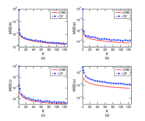
Figure 3: MSEs and CRBs associated with different sets of parameters vs. the number of subcarriers, $K$.

Figure 4: MSEs and CRBs associated with different sets of parameters vs. SNR.

We first examine the estimation accuracy of the channel parameters $\{\theta_{l},\phi_{l},\tau_{l},\alpha_{l}\}$. Mean square errors (MSEs) are calculated separately for each set of parameters, i.e.

$$\text{MSE}(\theta)= \|\boldsymbol{\theta}-\boldsymbol{\hat{\theta}}\|_{2}^{2}\quad\text{MSE}(\phi)=\|\boldsymbol{\phi}-\boldsymbol{\hat{\phi}}\|_{2}^{2}$$

$$\text{MSE}(\tau)= \|\boldsymbol{\tau}-\boldsymbol{\hat{\tau}}\|_{2}^{2}\quad\text{MSE}(\alpha)=\|\boldsymbol{\alpha}-\boldsymbol{\hat{\alpha}}\|_{2}^{2}$$

where $\boldsymbol{\theta}\triangleq[\theta_{1}\phantom{0}\ldots\phantom{0}\theta_{L}]^{T}$, $\boldsymbol{\phi}\triangleq[\phi_{1}\phantom{0}\ldots\phantom{0}\phi_{L}]^{T}$, $\boldsymbol{\tau}\triangleq[\tau_{1}\phantom{0}\ldots\phantom{0}\tau_{L}]^{T}$, and $\boldsymbol{\alpha}\triangleq[\alpha_{1}\phantom{0}\ldots\phantom{0}\alpha_{L}]^{T}$. Fig. 3 plots the MSEs of our proposed method as a function of the number of subcarriers used for training, $K$, where we set $M=6$, $T=6$, and $\text{SNR}=10\text{dB}$. The CRB results for different sets of parameters are also included for comparison. We see that our proposed method yields accurate estimates of the channel parameters even for small values of $M$, $T$, and $K$. This result indicates that our proposed method is able to achieve a substantial training overhead reduction. We also notice that the MSEs attained by our proposed method are very close to their corresponding CRBs, particularly for the AoA, AoD, and the time delay parameters. This result corroborates the optimality of the proposed method. As indicated earlier, the optimality of the proposed method comes from the fact that the ASL and the correlation-based scheme used in our proposed method are all maximum likelihood estimators under mild conditions. Specifically, it has been shown in [34] that the ALS yields maximum likelihood estimates and achieves its associated CRB in the presence of zero-mean i.i.d. Gaussian noise. We also proved that the simple correlation-based scheme employed in the second stage of our proposed method is a maximum likelihood estimator, provided that the estimator errors of the factor matrices are i.i.d. Gaussian random variables. Although the estimator errors may not strictly follow an i.i.d. Gaussian distribution, the correlation-based scheme is still an effective estimator that achieves near-optimality. Lastly, we observe that our proposed method fails when the number of subcarriers $K\leq 2$. This is because, for the case where $T=6>L$ and $M=6>L$, Kruskal’s condition is satisfied only if $K\geq 2$. Thus our result roughly coincides with our previous analysis regarding the uniqueness of the CP decomposition. Fig. 4 depicts the MSEs and CRBs vs. SNR, where we set $T=6$, $M=6$, and $K=6$. From Fig. 4, we see that the CRBs decrease exponentially with increasing SNR, and the estimation accuracy achieved by our proposed method has similar tendency as the CRBs. The MSEs attained by our proposed method, again, are close to their corresponding CRBs, except in the low SNR regime.

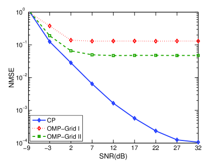
Figure 5: NMSEs of respective algorithms vs. SNR, $M=6$, $T=6$, $K=6$.

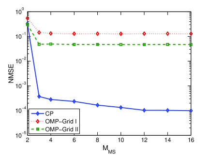
Figure 6: NMSEs of respective algorithms vs. the number of sub-frames $M$, $T=6$, $K=6$.

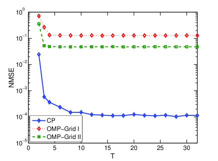
Figure 7: NMSEs of respective algorithms vs. the number of frames $T$, $M=6$, $K=6$.

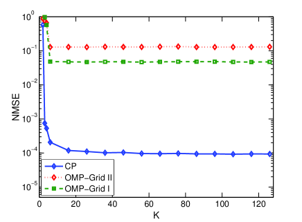
Figure 8: NMSEs of respective algorithms vs. the number of subcarriers for training $K$, $M=6$, $T=6$.

We now examine the channel estimation performance of our proposed method and its comparison with the compressed sensing method discussed in Section VI. Specifically, an orthogonal matching pursuit (OMP) algorithm is employed to solve the sparse signal recovery problem (54). Note that the dimension of the signal to be recovered in (54) is equal to $N_{1}N_{2}N_{3}$, where $N_{1}$, $N_{2}$, and $N_{3}$ denote the number of grid points used to discretize the AoA, AoD, and time delay domain, respectively. For a typical choice of $N_{1}=32$, $N_{2}=64$ and $N_{3}=32$, the dimension of the signal is of order $\mathcal{O}(10^{4})$. In this case, more sophisticated sparse recovery algorithms such as the fast iterative shrinkage-thresholding algorithm (FISTA) have a prohibitive computational complexity and thus are not included. Also, for the OMP, we employ two different grids to discretize the continuous parameter space: the first grid (referred to as Grid-I) discretizes the AoA-AoD-time delay space into $64\times 128\times 256$ grid points, and the second grid (referred to as Grid-II) discretizes the AoA-AoD-time delay space into $128\times 256\times 512$ grid points.

In Fig. 5, we show the NMSE results for our proposed method and the OMP algorithm as a function of SNR, where we set $M=6$, $T=6$, and $K=6$. Here the NMSE is calculated as

$$\text{NMSE}=\frac{\sum_{k=1}^{K}\|\boldsymbol{H}_{k}-\boldsymbol{\hat{H}}_{k}\|_{F}^{2}}{\sum_{k=1}^{K}\|\boldsymbol{H}_{k}\|_{F}^{2}}$$ (57)

where $\boldsymbol{H}_{k}$ denotes the frequency-domain channel matrix associated with the $k$th subcarrier, and $\boldsymbol{\hat{H}}_{k}$ is its estimate. We see that our proposed method achieves a substantial performance improvement over the compressed sensing algorithm. The performance gain is primarily due to the following two reasons. First, unlike compressed sensing techniques, our proposed CP decomposition-based method is essentially a gridless approach which is free from grid discretization errors. Second, the CP decomposition-based method captures the intrinsic multi-dimensional structure of the multiway data, which helps lead to a performance improvement. From Fig. 6 to Fig. 8, we plot the NMSEs of respective methods vs. $M$, $T$, and $K$, respectively, where the SNR is set to 20dB. These results, again, demonstrate the superiority of the proposed method over the compressed sensing method. We also observe that these results corroborate our theoretical analysis concerning the uniqueness of the CP decomposition. For example, in Fig. 6, since we have $T=6>L$ and $K=6>L$, we only need $M\geq 2$ to satisfy Kruskal’s condition. We see that our proposed method achieves an accurate channel estimate only when $M>2$, which roughly coincides with our analysis.

Table I shows the average run times of our proposed method and the OMP method. To provide a glimpse of other more sophisticated compressed sensing method’s computational complexity, the average run times of the FISTA are also included, from which we can see that sophisticated compressed sensing methods have a prohibitive computational complexity, and thus are not suitable for our channel estimation problem. We also see that our proposed method has a computational complexity as low as the OMP method. It takes similar run times as the OMP method which employs the coarser grid of the two choices, meanwhile achieving a much higher estimation accuracy than the OMP method that uses the finer grid.

TABLE I: Average run times of respective algorithms: $T=6$, $M=6$, $K=6$, and $\text{SNR}=20\text{dB}$.

ALG	Grid	NMSE	Average Run Time(s)
OMP	$64\times 128\times 256$	$2.3e-1$	$0.2$
	$160\times 320\times 640$	$3.5e-2$	$0.8$
FISTA	$32\times 64\times 128$	$2.3e-1$	$9e2$
	$64\times 128\times 256$	$9e-2$	$6e3$
CP	-	$1.2e-4$	$0.2$

IX Conclusions

We proposed a CP decomposition-based method for downlink channel estimation in mm-Wave MIMO-OFDM systems, where wideband mmWave channels with frequency selectivity were considered. The proposed method exploited the intrinsic multi-dimensional structure of the multiway data received at the BS. Specifically, the received signal at the BS was expressed as a third-order tensor. We showed that the tensor has a form of a low-rank CP decomposition, and the channel parameters can be easily extracted from the decomposed factor matrices. The uniqueness of the CP decomposition was investigated, which revealed that the uniqueness of the CP decomposition can be guaranteed even with a small number of measurements. Thus the proposed method is able to achieve a substantial training overhead reduction. CRB results for channel parameters were also developed. We compared our proposed method with a compressed sensing-based channel estimation method. Simulation results showed that our proposed method presents a clear performance advantage over the compressed sensing method in terms of both estimation accuracy and computational complexity.

Appendix A

In (38), for the $l$th column, we have

$$\boldsymbol{\hat{a}}_{l}=\lambda_{l}\boldsymbol{\tilde{a}}_{\rm{MS}}(\theta_{l})+\boldsymbol{e}_{l}$$ (58)

where $\theta_{l}$ and $\lambda_{l}$ are unknown parameters. We assume $\boldsymbol{e}_{l}$ satisfies circularly symmetric complex Gaussian distribution with zero mean and covariance matrix $\epsilon^{2}\boldsymbol{I}$. Thus the log-likelihood function is given by

$$L({\theta_{l}},{\lambda_{l}}) =-{M_{\rm MS}}\ln(\pi{\epsilon^{2}})-\frac{1}{{{\epsilon^{2}}}}\left\|{{{{\boldsymbol{\hat{a}}}}_{l}}-{\lambda_{l}}{{{\boldsymbol{\tilde{a}}}}_{{\rm{MS}}}}({\theta_{l}})}\right\|_{F}^{2}$$

$$\propto-\left\|{{{{\boldsymbol{\hat{a}}}}_{l}}-{\lambda_{l}}{{{\boldsymbol{\tilde{a}}}}_{{\rm{MS}}}}({\theta_{l}})}\right\|_{2}^{2}$$

Given a fixed $\theta_{l}$, the optimal $\lambda_{l}$ can be obtained by taking the partial derivative of the log-likelihood function with respect to $\lambda_{l}$ and setting the partial derivative equal to zero, i.e.

$$\frac{{\partial L({\theta_{l}},{\lambda_{l}})}}{{\partial{\lambda_{l}^{*}}}}={({{{\boldsymbol{\hat{a}}}}_{l}}-{\lambda_{l}}{{{\boldsymbol{\tilde{a}}}}_{{\rm{MS}}}}({\theta_{l}}))^{T}}{{{\boldsymbol{\tilde{a}}}}_{{\rm{MS}}}^{*}}({\theta_{l}})=0$$

which leads to

$$\lambda_{l}^{\star}=\frac{{{{{\boldsymbol{\hat{a}}}}_{l}}^{T}{{{\boldsymbol{\tilde{a}}}}_{{\rm{MS}}}^{*}}({\theta_{l}})}}{{{{\left\|{{{{\boldsymbol{\tilde{a}}}}_{{\rm{MS}}}}({\theta_{l}})}\right\|}^{2}}}}$$

Note that (58) can be rewritten as

$${\left\|{{{{\boldsymbol{\hat{a}}}}_{l}}}\right\|^{2}}={\lambda_{l}}{\boldsymbol{\hat{a}}}_{l}^{H}{{{\boldsymbol{\tilde{a}}}}_{{\rm{MS}}}}({\theta_{l}})+{\boldsymbol{\hat{a}}}_{l}^{H}{{\boldsymbol{e}}_{l}}$$

Then the log-likelihood function becomes

$$L({\theta_{l}},{\lambda_{l}}) \propto-{\left\|{{{\left\|{{{{\boldsymbol{\hat{a}}}}_{l}}}\right\|}^{2}}-{\lambda_{l}}{\boldsymbol{\hat{a}}}_{l}^{H}{{{\boldsymbol{\tilde{a}}}}_{{\rm{MS}}}}({\theta_{l}})}\right\|^{2}}$$ (59)

Substituting $\lambda_{l}^{\star}$ into the above log-likelihood function, we arrive at

$$L({\theta_{l}},\lambda_{l}^{\star})\propto-\left\|{{{\left\|{{{{\boldsymbol{\hat{a}}}}_{l}}}\right\|}^{2}}-\frac{{{{\left|{{\boldsymbol{\hat{a}}}_{l}^{H}{{{\boldsymbol{\tilde{a}}}}_{{\rm{MS}}}}({\theta_{l}})}\right|}^{2}}}}{{{{\left\|{{{{\boldsymbol{\tilde{a}}}}_{{\rm{MS}}}}({\theta_{l}})}\right\|}^{2}}}}}\right\|^{2}$$ (60)

$$\propto-\left\|{1-\frac{{{{\left|{{\boldsymbol{\hat{a}}}_{l}^{H}{{{\boldsymbol{\tilde{a}}}}_{{\rm{MS}}}}({\theta_{l}})}\right|}^{2}}}}{{{{\left\|{{{{\boldsymbol{\tilde{a}}}}_{{\rm{MS}}}}({\theta_{l}})}\right\|}^{2}}{{\left\|{{{{\boldsymbol{\hat{a}}}}_{l}}}\right\|}^{2}}}}}\right\|^{2}$$ (61)

Due to the Cauchy-Schwarz inequality, we have

$$0\leq\frac{{{{\left|{{\boldsymbol{\hat{a}}}_{l}^{H}{{{\boldsymbol{\tilde{a}}}}_{{\rm{MS}}}}({\theta_{l}})}\right|}^{2}}}}{{{{\left\|{{{{\boldsymbol{\tilde{a}}}}_{{\rm{MS}}}}({\theta_{l}})}\right\|}^{2}}{{\left\|{{{{\boldsymbol{\hat{a}}}}_{l}}}\right\|}^{2}}}}\leq 1$$

Therefore maximizing the log-likelihood with respect to $\theta_{l}$ is equivalent to

$$\theta_{l}^{\star}=\mathop{\arg\max}\limits_{{\theta_{l}}}L({\theta_{l}},\lambda_{l}^{\star})=\mathop{\arg\max}\limits_{{\theta_{l}}}\frac{{{{\left|{{\boldsymbol{\hat{a}}}_{l}^{H}{{{\boldsymbol{\tilde{a}}}}_{{\rm{MS}}}}({\theta_{l}})}\right|}^{2}}}}{{{{\left\|{{{{\boldsymbol{\hat{a}}}}_{l}}}\right\|}^{2}}{{\left\|{{{{\boldsymbol{\tilde{a}}}}_{{\rm{MS}}}}({\theta_{l}})}\right\|}^{2}}}}$$ (62)

The proof is completed here.

Appendix B

For a uniform linear array, the steering vector $\boldsymbol{a}_{\text{MS}}(\theta_{i})$ can be written as

$$\boldsymbol{a}_{\text{MS}}(\theta_{i})\triangleq[1\phantom{0}e^{j(2\pi/\lambda)d\text{sin}(\theta_{i})}\phantom{0}\ldots\phantom{0}e^{j(N_{\text{MS}}-1)(2\pi/\lambda)d\text{sin}(\theta_{i})}]^{T}$$

where $\lambda$ is the signal wavelength, and $d$ denotes the distance between neighboring antenna elements. We assume each entry of $\boldsymbol{Q}\in\mathbb{C}^{N_{\text{MS}}\times M}$ is chosen uniformly from a unit circle scaled by a constant $1/N_{\text{MS}}$, i.e. $q_{m,n}=(1/N_{\text{MS}})e^{j\vartheta_{m,n}}$, where $\vartheta_{m,n}\in[-\pi,\pi]$ follows a uniform distribution. Let $a_{m,i}\triangleq\boldsymbol{q}_{m}^{T}\boldsymbol{a}_{\text{MS}}(\theta_{i})$ denote the $(m,i)$th entry of $\boldsymbol{A}$, in which $\boldsymbol{q}_{m}$ denotes the $m$th column of $\boldsymbol{Q}$. It can be readily verified that ${\mathbb{E}}[a_{m,i}]=0,\forall m,i$ and

$${\mathbb{E}}[a_{m,i}a_{n,j}^{\ast}]=\begin{cases}0&m\neq n\\ \frac{1}{N_{\text{MS}}^{2}}\boldsymbol{a}_{\text{MS}}^{H}(\theta_{j})\boldsymbol{a}_{\text{MS}}(\theta_{i})&m=n\end{cases}$$ (63)

When the number of antennas at the MS is sufficiently large, the steering vectors $\{\boldsymbol{a}_{\text{MS}}(\theta_{i})\}$ become mutually quasi-orthogonal, i.e. $(1/N_{\text{MS}})\boldsymbol{a}_{\text{MS}}^{H}(\theta_{j})\boldsymbol{a}_{\text{MS}}(\theta_{j})\rightarrow\delta(\theta_{i}-\theta_{j})$, which implies that the entries of $\boldsymbol{A}$ are uncorrelated with each other. On the other hand, according to the central limit theorem, we know that each entry $a_{m,i}$ approximately follows a Gaussian distribution. Therefore entries of $\boldsymbol{A}$ can be considered as i.i.d. Gaussian variables with zero mean and variance $1/N_{\text{MS}}$. Thus we can reach that the k-rank of $\boldsymbol{A}$ is equivalent to the number of columns or the number of rows, whichever is smaller, with probability one.

Appendix C The Derivation of Cramér Rao Lower Bound

Consider the $M\times T\times K$ observation tensor $\boldsymbol{\mathcal{Y}}$ in (13)

$$\boldsymbol{\mathcal{Y}}=\sum_{l=1}^{L}\alpha_{l}\boldsymbol{\tilde{a}}_{\text{MS}}(\theta_{l})\circ\boldsymbol{\tilde{a}}_{\text{BS}}(\phi_{l})\circ\boldsymbol{g}(\tau_{l})+\boldsymbol{\mathcal{W}}$$ (64)

where $\{\alpha_{l},\theta_{l},\phi_{l},\tau_{l}\}$ are the unknown channel parameters to be estimated. We assume that entries of $\boldsymbol{\mathcal{W}}$ are i.i.d zero mean, circular symmetric Gaussian random variables with variance $\sigma^{2}$. For ease of exposition, let ${\boldsymbol{\theta}}\triangleq[\theta_{1}\phantom{0}\cdots\phantom{0}\theta_{L}]^{T}$, ${\boldsymbol{\phi}}\triangleq[\phi_{1}\phantom{0}\cdots\phantom{0}\phi_{L}]^{T}$, ${\boldsymbol{\tau}}\triangleq[\tau_{1}\phantom{0}\cdots\phantom{0}\tau_{L}]^{T}$, ${\boldsymbol{\alpha}}\triangleq[\alpha_{1}\phantom{0}\cdots\phantom{0}\alpha_{L}]^{T}$, and ${\boldsymbol{p}}\triangleq[\boldsymbol{\theta}^{T}\phantom{0}\boldsymbol{\phi}^{T}\phantom{0}\boldsymbol{\tau}^{T}\phantom{0}\boldsymbol{\alpha}^{T}]$. Thus, the log-likelihood function of $\boldsymbol{p}$ can be expressed as

$$L({\boldsymbol{p}})=f({\boldsymbol{\mathcal{Y}}};{\boldsymbol{A}},{\boldsymbol{B}},{\boldsymbol{C}})$$ (65)

where ${\boldsymbol{A}}$, ${\boldsymbol{B}}$ and ${\boldsymbol{C}}$, defined in (16), (17) and (18) respectively, are functions of the parameter vector $\boldsymbol{p}$, and $f({\boldsymbol{\mathcal{Y}}};{\boldsymbol{A}},{\boldsymbol{B}},{\boldsymbol{C}})$ is given by

$$f({\boldsymbol{\mathcal{Y}}};{\boldsymbol{A}},{\boldsymbol{B}},{\boldsymbol{C}})$$

$$=-MTK\ln(\pi{\sigma^{2}})-\frac{1}{{{\sigma^{2}}}}\left\|{{\boldsymbol{Y}}_{(1)}^{T}-({\boldsymbol{C}}\odot{\boldsymbol{B}}){{\boldsymbol{A}}^{T}}}\right\|_{F}^{2}$$

$$=-MTK\ln(\pi{\sigma^{2}})-\frac{1}{{{\sigma^{2}}}}\left\|{{\boldsymbol{Y}}_{(2)}^{T}-({\boldsymbol{C}}\odot{\boldsymbol{A}}){{\boldsymbol{B}}^{T}}}\right\|_{F}^{2}$$

$$=-MTK\ln(\pi{\sigma^{2}})-\frac{1}{{{\sigma^{2}}}}\left\|{{\boldsymbol{Y}}_{(3)}^{T}-({\boldsymbol{B}}\odot{\boldsymbol{A}}){{\boldsymbol{C}}^{T}}}\right\|_{F}^{2}$$

The complex Fisher information matrix (FIM) for $\boldsymbol{p}$ is given by [33, 34]

$${\boldsymbol{\Omega}}({\boldsymbol{p}})={\mathbb{E}}\left\{{{{\left(\frac{{\partial L({\boldsymbol{p}})}}{{\partial{\boldsymbol{p}}}}\right)}^{H}}\left(\frac{{\partial L({\boldsymbol{p}})}}{{\partial{\boldsymbol{p}}}}\right)}\right\}.$$ (66)

In the next, to calculate ${\boldsymbol{\Omega}}({\boldsymbol{p}})$, we first compute the partial derivative of $L({\boldsymbol{p}})$ with respect to $\boldsymbol{p}$ and then calculate the expectation with respect to $p(\boldsymbol{\mathcal{Y}};\boldsymbol{p})$.

C-A Partial Derivative of $L({\boldsymbol{p}})$ W.R.T $\boldsymbol{p}$

The partial derivative of $L({\boldsymbol{p}})$ with respect to $\theta_{l}$ can be computed as

$$\frac{{\partial L({\boldsymbol{p}})}}{{\partial{\theta_{l}}}}=\text{tr}\left\{{{{\left(\frac{{\partial L({\boldsymbol{p}})}}{{\partial{\boldsymbol{A}}}}\right)}^{T}}\frac{{\partial{\boldsymbol{A}}}}{{\partial{\theta_{l}}}}}+{{{\left(\frac{{\partial L({\boldsymbol{p}})}}{{\partial{{\boldsymbol{A}}^{*}}}}\right)}^{T}}\frac{{\partial{{\boldsymbol{A}}^{*}}}}{{\partial{\theta_{l}}}}}\right\}$$

where

$${{\frac{{\partial L({\boldsymbol{p}})}}{{\partial{\boldsymbol{A}}}}}}= \frac{1}{{{\sigma^{2}}}}{({\boldsymbol{Y}}_{(1)}^{T}-({\boldsymbol{C}}\odot{\boldsymbol{B}}){{\boldsymbol{A}}^{T}})^{H}}({\boldsymbol{C}}\odot{\boldsymbol{B}})$$

$${{\frac{{\partial L({\boldsymbol{p}})}}{{\partial{\boldsymbol{A}}^{*}}}}}= \left({{\frac{{\partial L({\boldsymbol{p}})}}{{\partial{\boldsymbol{A}}}}}}\right)^{*}$$

$$\frac{{\partial{\boldsymbol{A}}}}{{\partial{\theta_{l}}}}= \left[{\begin{array}[]{*{20}{c}}{\boldsymbol{0}}&\cdots&{{\boldsymbol{\tilde{a}}}_{l}}&\cdots&{\boldsymbol{0}}\end{array}}\right]$$ (69)

For a uniform linear array with the element spacing equal to half of the signal wavelength, we have ${{\boldsymbol{\tilde{a}}}_{l}}\triangleq j{{\boldsymbol{Q}}^{T}{{\boldsymbol{D}}_{{a}}}{{\boldsymbol{a}}_{\rm MS}(\theta_{l})}}$, and

$${{\boldsymbol{D}}_{{a}}}\triangleq\pi\cos(\theta_{l}){\text{diag}}(0,1,\cdots,N_{\text{MS}}-1)$$ (70)

Therefore, we have

$$\frac{{\partial L({\boldsymbol{p}})}}{{\partial{\theta_{l}}}}= {\boldsymbol{e}}_{l}^{T}\frac{1}{{{\sigma^{2}}}}{({\boldsymbol{C}}\odot{\boldsymbol{B}})^{T}}{({\boldsymbol{Y}}_{(1)}^{T}-({\boldsymbol{C}}\odot{\boldsymbol{B}}){{\boldsymbol{A}}^{T}})^{*}}{{{\boldsymbol{\tilde{a}}}}_{l}}$$

$$+{\boldsymbol{e}}_{l}^{T}\frac{1}{{{\sigma^{2}}}}{({\boldsymbol{C}}\odot{\boldsymbol{B}})^{H}}({\boldsymbol{Y}}_{(1)}^{T}-({\boldsymbol{C}}\odot{\boldsymbol{B}}){{\boldsymbol{A}}^{T}}){\boldsymbol{\tilde{a}}}_{l}^{*}$$

$$= 2{\mathop{\rm Re}\nolimits}\{{\boldsymbol{e}}_{l}^{T}\frac{1}{{{\sigma^{2}}}}{({\boldsymbol{C}}\odot{\boldsymbol{B}})^{T}}{({\boldsymbol{Y}}_{(1)}^{T}-({\boldsymbol{C}}\odot{\boldsymbol{B}}){{\boldsymbol{A}}^{T}})^{*}}{{{\boldsymbol{\tilde{a}}}}_{l}}\}$$

$$= 2{\mathop{\rm Re}\nolimits}\{{\boldsymbol{e}}_{l}^{T}\frac{1}{{{\sigma^{2}}}}{({\boldsymbol{C}}\odot{\boldsymbol{B}})^{T}}{({\boldsymbol{Y}}_{(1)}^{T}-({\boldsymbol{C}}\odot{\boldsymbol{B}}){{\boldsymbol{A}}^{T}})^{*}}{{{\boldsymbol{\tilde{A}}}}{\boldsymbol{e}}_{l}}\}$$ (71)

where ${\rm Re}\{\cdot\}$ is an operator which takes the real part of a complex number, ${\boldsymbol{e}}_{l}\in{\mathbb{C}}^{L\times 1}$ is the canonical vector whose non-zero entry is indexed as $l$, and

$${\boldsymbol{\tilde{A}}}\triangleq\left[{\begin{array}[]{*{20}{c}}{{{{\boldsymbol{\tilde{a}}}}_{1}}}&{{{{\boldsymbol{\tilde{a}}}}_{2}}}&\cdots&{{{{\boldsymbol{\tilde{a}}}}_{L}}}\end{array}}\right]$$ (73)

Similarly, we can obtain the partial derivatives with respect to other parameters as follows

$$\frac{{\partial L(\boldsymbol{p})}}{{\partial{\phi_{l}}}}=2{\mathop{\rm Re}\nolimits}\{{\boldsymbol{e}}_{l}^{T}\frac{1}{{{\sigma^{2}}}}{({\boldsymbol{C}}\odot{\boldsymbol{A}})^{T}}{({\boldsymbol{Y}}_{(2)}^{T}-({\boldsymbol{C}}\odot{\boldsymbol{A}}){{\boldsymbol{B}}^{T}})^{*}}{{\boldsymbol{\tilde{B}}}{{\boldsymbol{e}}_{l}}}\}$$

$$\frac{{\partial L({\boldsymbol{p}})}}{{\partial{\tau_{l}}}}=2{\mathop{\rm Re}\nolimits}\{{\boldsymbol{e}}_{l}^{T}\frac{1}{{{\sigma^{2}}}}{({\boldsymbol{B}}\odot{\boldsymbol{A}})^{T}}{({\boldsymbol{Y}}_{(3)}^{T}-({\boldsymbol{B}}\odot{\boldsymbol{A}}){{\boldsymbol{C}}^{T}})^{*}}{{\boldsymbol{\tilde{C}}}{\boldsymbol{e}}_{l}}\}$$

$$\frac{{\partial L({\boldsymbol{p}})}}{{\partial{\alpha_{l}}}}={\boldsymbol{e}}_{l}^{T}\frac{1}{{{\sigma^{2}}}}{({\boldsymbol{B}}\odot{\boldsymbol{A}})^{T}}{({\boldsymbol{Y}}_{(3)}^{T}-({\boldsymbol{B}}\odot{\boldsymbol{A}}){{\boldsymbol{C}}^{T}})^{*}}{{\boldsymbol{G}}{\boldsymbol{e}}_{l}}$$

where

$${\boldsymbol{\tilde{B}}} \triangleq\left[{\begin{array}[]{*{20}{c}}{{{{\boldsymbol{\tilde{b}}}}_{1}}}&{{{{\boldsymbol{\tilde{b}}}}_{2}}}&\cdots&{{{{\boldsymbol{\tilde{b}}}}_{L}}}\end{array}}\right]$$ (75)

$${\boldsymbol{\tilde{C}}} \triangleq\left[{\begin{array}[]{*{20}{c}}{{{{\boldsymbol{\tilde{c}}}}_{1}}}&{{{{\boldsymbol{\tilde{c}}}}_{2}}}&\cdots&{{{{\boldsymbol{\tilde{c}}}}_{L}}}\end{array}}\right]$$ (77)

$${\boldsymbol{G}} \triangleq\left[{\begin{array}[]{*{20}{c}}{{{{\boldsymbol{g}}}_{1}}}&{{{{\boldsymbol{g}}}_{2}}}&\cdots&{{{{\boldsymbol{g}}}_{L}}}\end{array}}\right]$$ (79)

in which ${{\boldsymbol{\tilde{b}}}_{l}}\triangleq j{{\boldsymbol{P}}^{T}{\boldsymbol{D}}_{b}{{\boldsymbol{a}}_{\rm BS}}(\phi_{l})}$, ${\boldsymbol{\tilde{c}}}_{l}\triangleq j{{\boldsymbol{D}}_{{c}}}{{\boldsymbol{c}}_{l}}$, and

$${\boldsymbol{D}}_{b} \triangleq\pi\cos(\phi_{l}){\text{diag}}(0,1,\cdots,N_{\text{BS}}-1)$$ (80)

$${{\boldsymbol{D}}_{c}} \triangleq-2\pi{\text{diag}}(0,f_{s}/\bar{K},\cdots,(K-1)f_{s}/\bar{K})$$ (81)

C-B Calculation of Fisher Information Matrix

We first calculate the entries in the principal minors of $\boldsymbol{\Omega}(\boldsymbol{p})$. For instance, the $(l_{1},l_{2})$th entry of

$${\mathbb{E}}\left\{{{{\left(\frac{{\partial L({\boldsymbol{p}})}}{{\partial{\boldsymbol{\theta}}}}\right)}^{H}}\left(\frac{{\partial L({\boldsymbol{p}})}}{{\partial{\boldsymbol{\theta}}}}\right)}\right\}.$$

is given by

$${\mathbb{E}}\left\{{{{\left(\frac{{\partial L({\boldsymbol{p}})}}{{\partial{\theta_{{l_{1}}}}}}\right)}^{*}}\left(\frac{{\partial L({\boldsymbol{p}})}}{{\partial{\theta_{{l_{2}}}}}}\right)}\right\}$$

$$=4{\mathbb{E}}\left[{{\mathop{\rm Re}\nolimits}\{{\boldsymbol{e}}_{{l_{1}}}^{T}{{{\boldsymbol{N}}}^{a}}{{\boldsymbol{e}}_{{l_{1}}}}\}{\mathop{\rm Re}\nolimits}\{{\boldsymbol{e}}_{{l_{2}}}^{T}{{{\boldsymbol{N}}}^{a}}{{\boldsymbol{e}}_{{l_{2}}}}\}}\right]$$

$$={\mathbb{E}}\left[{\left({{{\boldsymbol{N}}}^{{a}}}({l_{1}},{l_{1}})+{{{\boldsymbol{N}}}^{{a}}}{{({l_{1}},{l_{1}})}^{*}}\right)\left({{{\boldsymbol{N}}}^{{a}}}({l_{2}},{l_{2}})+{{{\boldsymbol{N}}}^{{a}}}{{({l_{2}},{l_{2}})}^{*}}\right)}\right]$$

where ${{{\boldsymbol{N}}}^{{a}}}({l_{1}},{l_{1}})$ stands for the $(l_{1},l_{1})$th entry of ${{{\boldsymbol{N}}}^{{a}}}\in{\mathbb{C}}^{L\times L}$ and

$${{{\boldsymbol{N}}}^{a}} \triangleq\frac{1}{{{\sigma^{2}}}}{({\boldsymbol{C}}\odot{\boldsymbol{B}})^{T}}{({\boldsymbol{Y}}_{(1)}^{T}-({\boldsymbol{C}}\odot\boldsymbol{B}){{\boldsymbol{A}}^{T}})^{*}}{\boldsymbol{\tilde{A}}}$$

$$=\frac{1}{{{\sigma^{2}}}}{({\boldsymbol{C}}\odot{\boldsymbol{B}})^{T}}{({{\boldsymbol{W}}^{T}_{(1)}})^{*}}{\boldsymbol{\tilde{A}}}.$$

Letting ${{{\boldsymbol{n}}}^{a}}\triangleq\text{vec}({{{\boldsymbol{N}}}^{a}})$, we have

$${{{\boldsymbol{n}}}^{a}}=\left({\boldsymbol{\tilde{A}}}^{T}\otimes{({\boldsymbol{C}}\odot{\boldsymbol{B}})^{T}}\right){\text{vec}}({{\boldsymbol{W}}^{H}_{(1)}}).$$ (82)

where ${{\boldsymbol{W}}_{(1)}}$ is the mode-1 unfolding of $\boldsymbol{\mathcal{W}}$, thus ${\text{vec}}({{\boldsymbol{W}}^{H}_{(1)}})$ is a zero mean circularly symmetric complex Gaussian vector whose covariance matrix is given by $\sigma^{2}\boldsymbol{I}$. Since ${{{\boldsymbol{n}}}^{a}}$ is the linear transformation of ${\text{vec}}({{\boldsymbol{W}}^{H}_{(1)}})$, ${{{\boldsymbol{n}}}^{a}}$ also follows a circularly symmetric complex Gaussian distribution. Its covariance matrix ${\boldsymbol{C}}_{{{\boldsymbol{n}}}^{a}}\in{\mathbb{C}}^{L^{2}\times L^{2}}$ and second-order moments ${\boldsymbol{M}}_{{{\boldsymbol{n}}}^{a}}\in{\mathbb{C}}^{L^{2}\times L^{2}}$ are respectively given by

$$\boldsymbol{C}_{\boldsymbol{n}^{a}} ={\mathbb{E}}\left[(\boldsymbol{n}^{a})(\boldsymbol{n}^{a})^{H}\right]$$

$$=\frac{1}{\sigma^{2}}\left(\boldsymbol{\tilde{A}}^{T}\otimes{({\boldsymbol{C}}\odot{\boldsymbol{B}})^{T}}\right)\left(\boldsymbol{\tilde{A}}^{*}\otimes{(\boldsymbol{C}\odot\boldsymbol{B})^{*}}\right)$$

$$=\frac{1}{{{\sigma^{2}}}}\left(\boldsymbol{\tilde{A}}^{T}\boldsymbol{\tilde{A}}^{*}\right)\otimes\left({(\boldsymbol{C}\odot\boldsymbol{B})^{T}}{(\boldsymbol{C}\odot\boldsymbol{B})^{*}}\right)$$ (83)

and

$${\boldsymbol{M}}_{{{\boldsymbol{n}}}^{a}}={\mathbb{E}}\left[({{{\boldsymbol{n}}}^{a}})({{{\boldsymbol{n}}}^{a}})^{T}\right]=\boldsymbol{0}$$ (84)

Therefore, we have

$${\mathbb{E}}\left\{{{{\left(\frac{{\partial L(\boldsymbol{p})}}{{\partial{\theta_{{l_{1}}}}}}\right)}^{*}}\left(\frac{{\partial L(\boldsymbol{p})}}{{\partial{\theta_{{l_{2}}}}}}\right)}\right\}=2{\rm Re}\{{\boldsymbol{C}}_{{{\boldsymbol{n}}}^{a}}(m,n)\}$$ (85)

where $m\triangleq L(l_{1}-1)+l_{1}$ and $n\triangleq L(l_{2}-1)+l_{2}$. Similarly, we can arrive at

$${\mathbb{E}}\left\{{{{\left(\frac{{\partial L({\boldsymbol{p}})}}{{\partial{\phi_{{l_{1}}}}}}\right)}^{*}}\left(\frac{{\partial L({\boldsymbol{p}})}}{{\partial{\phi_{{l_{2}}}}}}\right)}\right\} =2{\mathop{\rm Re}\nolimits}\{{{\boldsymbol{C}}_{{{{\boldsymbol{n}}}^{b}}}}(m,n)\}$$

$${\mathbb{E}}\left\{{{{\left(\frac{{\partial L({\boldsymbol{p}})}}{{\partial{\tau_{{l_{1}}}}}}\right)}^{*}}\left(\frac{{\partial L(\boldsymbol{p})}}{{\partial{\tau_{{l_{2}}}}}}\right)}\right\} =2{\mathop{\rm Re}\nolimits}\{{\boldsymbol{C}}_{{{{\boldsymbol{n}}}^{c}}}(m,n)\}$$

$${\mathbb{E}}\left\{{{{\left(\frac{{\partial L({\boldsymbol{p}})}}{{\partial{\alpha_{{l_{1}}}}}}\right)}^{*}}\left(\frac{{\partial L(\boldsymbol{p})}}{{\partial{\alpha_{{l_{2}}}}}}\right)}\right\} ={\boldsymbol{C}}_{{{{\boldsymbol{\tilde{n}}}}^{c}}}(m,n)^{*},$$

in which

$${{\boldsymbol{C}}_{{{{\boldsymbol{n}}}^{b}}}}\triangleq\frac{1}{{{\sigma^{2}}}}\left(\boldsymbol{\tilde{B}}^{T}\boldsymbol{\tilde{B}}^{*}\right)\otimes\left({(\boldsymbol{C}\odot\boldsymbol{A})^{T}}{(\boldsymbol{C}\odot\boldsymbol{A})^{*}}\right)$$ (86)

$${{\boldsymbol{C}}_{{{{\boldsymbol{n}}}^{c}}}}\triangleq\frac{1}{{{\sigma^{2}}}}\left(\boldsymbol{\tilde{C}}^{T}\boldsymbol{\tilde{C}}^{*}\right)\otimes\left({(\boldsymbol{B}\odot\boldsymbol{A})^{T}}{(\boldsymbol{B}\odot\boldsymbol{A})^{*}}\right)$$ (87)

$${{\boldsymbol{C}}_{{{{\boldsymbol{\tilde{n}}}}^{c}}}}\triangleq\frac{1}{{{\sigma^{2}}}}\left(\boldsymbol{G}^{T}\boldsymbol{G}^{*}\right)\otimes\left({(\boldsymbol{B}\odot\boldsymbol{A})^{T}}{(\boldsymbol{B}\odot\boldsymbol{A})^{*}}\right)$$ (88)

For the elements in the off-principal minors of $\boldsymbol{\Omega}(\boldsymbol{p})$, such as the $(l_{1},l_{2})$th entry of

$${\mathbb{E}}\left\{{{{\left(\frac{{\partial L({\boldsymbol{p}})}}{{\partial{\boldsymbol{\theta}}}}\right)}^{H}}\left(\frac{{\partial L({\boldsymbol{p}})}}{{\partial{\boldsymbol{\phi}}}}\right)}\right\}.$$

is given by

$${\mathbb{E}}\left\{{{{\left(\frac{{\partial L({\boldsymbol{p}})}}{{\partial{\theta_{{l_{1}}}}}}\right)}^{*}}\left(\frac{{\partial L({\boldsymbol{p}})}}{{\partial{\phi_{{l_{2}}}}}}\right)}\right\}$$

$$=4{\mathbb{E}}\left[{{\mathop{\rm Re}\nolimits}\left\{{\bf{e}}_{{l_{1}}}^{T}{{{\boldsymbol{N}}}^{a}}{{\bf{e}}_{{l_{1}}}}\right\}{\mathop{\rm Re}\nolimits}\{{\bf{e}}_{{l_{2}}}^{T}{{{\boldsymbol{N}}}^{b}}{{\boldsymbol{e}}_{{l_{2}}}}\}}\right]$$

$$={\mathbb{E}}\left[{({{{\boldsymbol{N}}}^{{a}}}({l_{1}},{l_{1}})+{{{\boldsymbol{N}}}^{{a}}}{{({l_{1}},{l_{1}})}^{*}})({{{\boldsymbol{N}}}^{{b}}}({l_{2}},{l_{2}})+{{{\boldsymbol{N}}}^{{b}}}{{({l_{2}},{l_{2}})}^{*}})}\right]$$

$$=2{\mathop{\rm Re}\nolimits}\left\{{\boldsymbol{C}}_{{{{{\boldsymbol{n}}}^{a}}},{{{{\boldsymbol{n}}}^{b}}}}(m,n)\right\}$$

where

$${\boldsymbol{C}}_{{{{{\boldsymbol{n}}}^{a}}},{{{{\boldsymbol{n}}}^{b}}}} \triangleq{\mathbb{E}}\left[(\boldsymbol{n}^{a})(\boldsymbol{n}^{b})^{H}\right]$$

$$=\frac{1}{{{\sigma^{4}}}}{({\boldsymbol{\tilde{A}}}\otimes({\boldsymbol{C}}\odot{\boldsymbol{B}}))^{T}}{\boldsymbol{C}}_{{{\boldsymbol{w}}_{1}},{{\boldsymbol{w}}_{2}}}({{{\boldsymbol{\tilde{B}}}}^{*}}\otimes{({\boldsymbol{C}}\odot{\boldsymbol{A}})^{*}})$$ (89)

in which

$${\boldsymbol{C}}_{{{\boldsymbol{w}}_{1}},{{\boldsymbol{w}}_{2}}}\triangleq{\mathbb{E}}\{{\text{vec}}({\boldsymbol{W}}_{(1)}^{H}){\text{vec}}{({\boldsymbol{W}}_{(2)}^{T})^{T}}\}$$ (90)

Similarly, we can obtain

$${\mathbb{E}}\left\{{{{\left(\frac{{\partial f(\boldsymbol{p})}}{{\partial{\theta_{{l_{1}}}}}}\right)}^{*}}\left(\frac{{\partial f(\boldsymbol{p})}}{{\partial{\tau_{{l_{2}}}}}}\right)}\right\} =2{\rm{Re}}\{\boldsymbol{C}_{\boldsymbol{n}^{a},\boldsymbol{n}^{c}}(m,n)\}$$

$${\mathbb{E}}\left\{{{{\left(\frac{{\partial f(\boldsymbol{p})}}{{\partial{\theta_{{l_{1}}}}}}\right)}^{*}}\left(\frac{{\partial f(\boldsymbol{p})}}{{\partial{\alpha_{{l_{2}}}}}}\right)}\right\} =\boldsymbol{C}_{{\boldsymbol{n}}^{a},{\boldsymbol{\tilde{n}}}^{c}}(m,n)^{*}$$

$${\mathbb{E}}\left\{{{{\left(\frac{{\partial f(\boldsymbol{p})}}{{\partial{\phi_{{l_{1}}}}}}\right)}^{*}}\left(\frac{{\partial f(\boldsymbol{p})}}{{\partial{\tau_{{l_{2}}}}}}\right)}\right\} =2{\rm{Re}}\{\boldsymbol{C}_{{\boldsymbol{n}}^{b},{\boldsymbol{n}}^{c}}(m,n)\}$$

$${\mathbb{E}}\left\{{{{\left(\frac{{\partial f(\boldsymbol{p})}}{{\partial{\phi_{{l_{1}}}}}}\right)}^{*}}\left(\frac{{\partial f(\boldsymbol{p})}}{{\partial{\alpha_{{l_{2}}}}}}\right)}\right\} ={{\boldsymbol{C}}_{{\boldsymbol{n}}^{b},{\boldsymbol{\tilde{n}}}^{c}}}(m,n)^{*}$$

$${\mathbb{E}}\left\{{{{\left(\frac{{\partial f(\boldsymbol{p})}}{{\partial{\tau_{{l_{1}}}}}}\right)}^{*}}\left(\frac{{\partial f(\boldsymbol{p})}}{{\partial{\alpha_{{l_{2}}}}}}\right)}\right\} =\boldsymbol{C}_{{\boldsymbol{n}}^{c},{\boldsymbol{\tilde{n}}}^{c}}(m,n)^{*}$$

where

$${\boldsymbol{C}}_{{{{{\boldsymbol{n}}}^{a}}},{{{{\boldsymbol{n}}}^{c}}}}\triangleq\frac{1}{{{\sigma^{4}}}}{({\boldsymbol{\tilde{A}}}\otimes({\boldsymbol{C}}\odot{\boldsymbol{B}}))^{T}}{\boldsymbol{C}}_{{{\boldsymbol{w}}_{1}},{{\boldsymbol{w}}_{3}}}({{{\boldsymbol{\tilde{C}}}}^{*}}\otimes{({\boldsymbol{B}}\odot{\boldsymbol{A}})^{*}})$$

$${\boldsymbol{C}}_{{{{{\boldsymbol{n}}}^{a}}},{{{{\boldsymbol{\tilde{n}}}}^{c}}}}\triangleq\frac{1}{{{\sigma^{4}}}}{({\boldsymbol{\tilde{A}}}\otimes({\boldsymbol{C}}\odot{\boldsymbol{B}}))^{T}}{\boldsymbol{C}}_{{{\boldsymbol{w}}_{1}},{{\boldsymbol{w}}_{3}}}({{{\boldsymbol{G}}}^{*}}\otimes{({\boldsymbol{B}}\odot{\boldsymbol{A}})^{*}})$$

$${\boldsymbol{C}}_{{{{{\boldsymbol{n}}}^{b}}},{{{{\boldsymbol{n}}}^{c}}}}\triangleq\frac{1}{{{\sigma^{4}}}}{({\boldsymbol{\tilde{B}}}\otimes({\boldsymbol{C}}\odot{\boldsymbol{A}}))^{T}}{\boldsymbol{C}}_{{{\boldsymbol{w}}_{2}},{{\boldsymbol{w}}_{3}}}({{{\boldsymbol{\tilde{C}}}}^{*}}\otimes{({\boldsymbol{B}}\odot{\boldsymbol{A}})^{*}})$$

$${\boldsymbol{C}}_{{{{{\boldsymbol{n}}}^{b}}},{{{{\boldsymbol{\tilde{n}}}}^{c}}}}\triangleq\frac{1}{{{\sigma^{4}}}}{({\boldsymbol{\tilde{B}}}\otimes({\boldsymbol{C}}\odot{\boldsymbol{A}}))^{T}}{\boldsymbol{C}}_{{{\boldsymbol{w}}_{2}},{{\boldsymbol{w}}_{3}}}({{{\boldsymbol{G}}}^{*}}\otimes{({\boldsymbol{B}}\odot{\boldsymbol{A}})^{*}})$$

$${\boldsymbol{C}}_{{{{{\boldsymbol{n}}}^{c}}},{{{{\boldsymbol{\tilde{n}}}}^{c}}}}\triangleq\frac{1}{{{\sigma^{2}}}}{({\boldsymbol{\tilde{C}}}\otimes({\boldsymbol{B}}\odot{\boldsymbol{A}}))^{T}}({{{\boldsymbol{G}}}^{*}}\otimes{({\boldsymbol{B}}\odot{\boldsymbol{A}})^{*}})$$

in which

$$\boldsymbol{C}_{\boldsymbol{w}_{1},\boldsymbol{w}_{3}} \triangleq{\mathbb{E}}\{\text{vec}({\boldsymbol{W}}_{(1)}^{H}){\text{vec}}{({\boldsymbol{W}}_{(3)}^{T})^{T}}\}$$

$$\boldsymbol{C}_{{\boldsymbol{w}}_{2},{\boldsymbol{w}}_{3}} \triangleq{\mathbb{E}}\{{\text{vec}}({\boldsymbol{W}}_{(2)}^{H}){\text{vec}}{({\boldsymbol{W}}_{(3)}^{T})^{T}}\}.$$

The computation of $\boldsymbol{C}_{{\boldsymbol{w}}_{1},{\boldsymbol{w}}_{2}}$ is elaborated as follows. Note that the $(m,t,k)$th entry in $\boldsymbol{\mathcal{W}}\in{\mathbb{C}}^{M\times T\times K}$ corresponds to the $(m,t+(k-1)T)$th entry of ${\boldsymbol{W}}_{(1)}$ and also corresponds to the $(t,m+(k-1)M)$th entry of ${\boldsymbol{W}}_{(2)}$. Furthermore, the $(m,t+(k-1)T)$th entry of ${\boldsymbol{W}}_{(1)}$ corresponds to the $(t+(k-1)T+(m-1)TK)$th entry of ${{{\text{vec}}}({{{\boldsymbol{W}}}^{H}_{(1)}})}$ and the $(t,m+(k-1)M)$th entry of ${\boldsymbol{W}}_{(2)}$ corresponds to the $(m+(k-1)M+(t-1)MK)$th entry of ${{{\text{vec}}}({{{\boldsymbol{W}}}^{T}_{(2)}})}$. Since entries in $\boldsymbol{\mathcal{W}}$ are i.i.d. random variables, i.e.,

$${\mathbb{E}}\{{w_{{m_{1}},{t_{1}},{k_{1}}}}w_{{m_{2}},{t_{2}},{k_{2}}}^{*}\}=\left\{{\begin{aligned} &{{\sigma^{2}};{m_{1}}={m_{2}},{t_{1}}={t_{2}},{k_{1}}={k_{2}}}\\ &{0;\text{otherwise}}\end{aligned}}\right.$$

where ${w_{{m},{t},{k}}}$ represents the $(m,t,k)$th entry of $\boldsymbol{\mathcal{W}}$. Therefore, in $\boldsymbol{C}_{{\boldsymbol{w}}_{1},{\boldsymbol{w}}_{2}}\in{\mathbb{C}}^{TKM\times MKT}$, the number of nonzero entries is $MTK$ and the corresponding indexes, $\{(n_{1},n_{2})|\boldsymbol{C}_{{\boldsymbol{w}}_{1},{\boldsymbol{w}}_{2}}(n_{1},n_{2})\neq 0\}$, is equal to

$$\{(n_{1},n_{2})| n_{1}=t+(k-1)T+(m-1)TK,$$

$$n_{2}=m+(k-1)M+(t-1)MK,\forall m,t,k\}$$

Similarly, the index of the nonzero elements in $\boldsymbol{C}_{{\boldsymbol{w}}_{1},{\boldsymbol{w}}_{3}}\in{\mathbb{C}}^{TKM\times MTK}$ and $\boldsymbol{C}_{{\boldsymbol{w}}_{2},{\boldsymbol{w}}_{3}}\in{\mathbb{C}}^{MKT\times MTK}$ are respectively belongs to

$$\{(n_{1},n_{2})| n_{1}=t+(k-1)T+(m-1)TK,$$

$$n_{2}=m+(t-1)M+(k-1)MT,\forall m,t,k\}$$

and

$$\{(n_{1},n_{2})| n_{1}=m+(k-1)M+(t-1)MK,$$

$$n_{2}=m+(t-1)M+(k-1)MT,\forall m,t,k\}$$

C-C Cramér Rao bound

After obtaining the fisher information matrix, the CRB for the parameters $\boldsymbol{p}$ can be calculated as [33]

$${\rm{CRB}}(\boldsymbol{p})=\boldsymbol{\Omega}^{-1}(\boldsymbol{p})$$ (91)

References

[1]
S. Rangan, T. S. Rappaport, and E. Erkip, “Millimeter-wave cellular wireless
networks: potentials and challenges,” Proc. IEEE, vol. 102, no. 3,
pp. 366–385, March 2014.
[2]
A. Ghosh, T. A. Thomas, M. C. Cudak, R. Ratasuk, P. Moorut, F. W. Vook, T. S.
Rappaport, G. R. MacCartney, S. Sun, and S. Nie, “Millimeter-wave enhanced
local area systems: a high-data-rate approach for future wireless networks,”
IEEE J. Sel. Areas Commun., vol. 32, no. 6, pp. 1152–1163, June 2014.
[3]
A. L. Swindlehurst, E. Ayanoglu, P. Heydari, and F. Capolino, “Millimeter-wave
massive MIMO: the next wireless revolution?” IEEE Commun. Mag.,
vol. 52, no. 9, pp. 56–62, September 2014.
[4]
A. Alkhateeb, J. Mo, N. Gonzalez-Prelcic, and R. Heath, “MIMO precoding and
combining solutions for millimeter-wave systems,” IEEE Commun. Mag.,
vol. 52, no. 12, pp. 122–131, December 2014.
[5]
O. E. Ayach, S. Rajagopal, S. Abu-Surra, Z. Pi, and R. Heath, “Spatially
sparse precoding in millimeter wave MIMO systems,” IEEE Trans.
Wireless Commun., vol. 13, no. 3, pp. 1499–1513, March 2014.
[6]
A. Alkhateeb, G. Leus, and R. Heath, “Limited feedback hybrid precoding for
multi-user millimeter wave systems,” IEEE Trans. Wireless Commun.,
vol. 14, no. 11, pp. 6481–6494, November 2015.
[7]
X. Gao, L. Dai, S. Han, C.-L. I, and R. W. Heath, “Energy-efficient hybrid
analog and digital precoding for mmwave MIMO systems with large antenna
arrays,” IEEE J. Sel. Areas Commun., vol. 34, no. 4, pp. 998–1009,
April 2016.
[8]
M. N. Kulkarni, A. Ghosh, and J. G. Andrews, “A comparison of MIMO
techniques in downlink millimeter wave cellular networks with hybrid
beamforming,” IEEE Trans. Commun., vol. 64, no. 5, pp. 1952–1967,
May 2016.
[9]
S. Hur, T. Kim, D. J. Love, J. V. Krogmeier, T. A. Thomas, and A. Ghosh,
“Millimeter wave beamforming for wireless backhaul and access in small cell
networks,” IEEE Trans. Commun., vol. 61, no. 10, pp. 4391–4403,
October 2013.
[10]
T. Kim and D. J. Love, “Virtual AoA and AoD estimation for sparse
millimeter wave MIMO channels,” in Proc. 16th IEEE Inter. Workshop
on Signal Process. Advances in Wireless Commun. (SPAWC), Stockholm, Sweden,
June 28 - July 1 2015, pp. 146–150.
[11]
J. Wang, Z. Lan, C.-W. Pyo, T. Baykas, C.-S. Sum, M. A. Rahman, J. Gao,
R. Funada, F. Kojima, H. Harada, and S. Kato, “Beam codebook based
beamforming protocol for multi-Gbps millimeter-wave WPAN systems,”
IEEE J. Sel. Areas Commun., vol. 27, no. 8, pp. 1390–1399, October
2009.
[12]
Y. M. Tsang, A. S. Y. Poon, and S. Addepalli, “Coding the beams: improving
beamforming training in mmWave communication system,” in Proc. 2011
IEEE Globel Commun. Conf. (Globecom), Houston, Texas, USA, December 5-9
2011.
[13]
A. Alkhateeb, G. Leus, and R. Heath, “Compressed sensing based multi-user
millimeter wave systems: How many measurements are needed?” in Proc.
40th IEEE Inter. Conf. on Acoust., Speech and Signal Process. (ICASSP),
Brisbane, Australia, April 19-24 2015, pp. 2909–2913.
[14]
A. Alkhateeb, O. E. Ayach, G. Leus, and R. Heath, “Channel estimation and
hybrid precoding for millimeter wave cellular systems,” IEEE J. Sel.
Topics Signal Process., vol. 8, no. 5, pp. 831–846, October 2014.
[15]
P. Schniter and A. Sayeed, “Channel estimation and precoder design for
millimeter-wave communications: The sparse way,” in Proc. 48th
Asilomar Conf. Signals, Syst. Comput., Pacific Grove, California, USA,
November 2-5 2014, pp. 273–277.
[16]
Z. Zhou, J. Fang, L. Yang, H. Li, Z. Chen, and S. Li, “Channel estimation for
millimeter-wave multiuser MIMO systems via PARAFAC decomposition,”
IEEE Trans. Wireless Commun., to appear.
[17]
D. Ramasamy, S. Venkateswaran, and U. Madhow, “Compressive adaptation of large
steerable arrays,” in Proc. 2012 Information Theory and Applications
Workshop (ITA), San Diego, California, USA, February 5-10 2012, pp.
234–239.
[18]
——, “Compressive tracking with 1000-element arrays: A framework for
multi-gbps mm wave cellular downlinks,” in Proc. 50th Annual Allerton
Conference on Commun., Control, and Comput., October 2012, pp. 690–697.
[19]
Z. Marzi, D. Ramasamy, and U. Madhow, “Compressive channel estimation and
tracking for large arrays in mm-Wave picocells,” IEEE J. Sel. Topics
Signal Process., vol. 10, no. 3, pp. 514–527, April 2016.
[20]
H. Xie, F. Gao, S. Zhang, and S. Jin, “A unified transmission strategy for
TDD/FDD massive MIMO systems with spatial basis expansion model,”
IEEE Trans. Veh. Technol., to appear.
[21]
A. Alkhateeb and R. W. Heath, “Frequency selective hybrid precoding for
limited feedback millimeter wave systems,” IEEE Trans. Commun.,
vol. 64, no. 5, pp. 1801–1818, May 2016.
[22]
Z. Gao, C. Hu, L. Dai, and Z. Wang, “Channel estimation for millimeter-wave
massive MIMO with hybrid precoding over frequency-selective fading
channels,” IEEE Commun. Lett., vol. 20, no. 6, pp. 1259–1262, June
2016.
[23]
Y. C. Pati, R. Rezaiifar, and P. S. Krishnaprasad, “Orthogonal matching
pursuit: recursive function approximation with applications to wavelet
decomposition,” in Proc. 27th Annu. Asilomar Conf. Signals, Systems,
and Computers, vol. 1, Pacific Grove, CA, Nov. 1993, pp. 40–44.
[24]
T. G. Kolda and B. W. Bader, “Tensor decompositions and applications,”
SIAM Rev., vol. 51, no. 3, pp. 455–500, August 2009.
[25]
T. G. Kolda, Multilinear operators for higher-order
decompositions. United States.
Department of Energy, 2006.
[26]
A. Cichocki, D. P. Mandic, A. H. Phan, C. F. Caiafa, G. Zhou, Q. Zhao, and
L. D. Lathauwer, “Tensor decompositions for signal processing applications:
From two-way to multiway component analysis,” IEEE Signal Process.
Mag., vol. 32, no. 2, pp. 145–163, March 2015.
[27]
M. R. Akdeniz, Y. Liu, M. K. Samimi, S. Sun, S. Rangan, T. S. Rappaport, and
E. Erkip, “Millimeter wave channel modeling and cellular capacity
evaluation,” IEEE J. Sel. Areas Commun., vol. 32, no. 6, pp.
1164–1179, June 2014.
[28]
J. A. Bazerque, G. Mateos, and G. B. Giannakis, “Rank regularization and
bayesian inference for tensor completion and extrapolation,” IEEE
Trans. Signal Process., vol. 61, no. 22, pp. 5689–5703, November 2013.
[29]
P. Rai, Y. Wang, S. Guo, G. Chen, D. Dunson, and L. Carin, “Scalable
Bayesian low-rank decomposition of incomplete multiway tensors,” in
Proceedings of the 31st International Conference on Machine Learning
(ICML-14), vol. 32, Beijing, China, 2014, pp. 1800–1808.
[30]
Q. Zhao, L. Zhang, and A. Cichocki, “Bayesian CP factorization of
incomplete tensors with automatic rank determination,” IEEE
Transactions on Pattern Analysis and Machine Intelligence, vol. 37, no. 9,
pp. 1751–1763, Sept. 2015.
[31]
J. B. Kruskal, “Three-way arrays: rank and uniqueness of trilinear
decompositions, with application to arithmetic complexity and statistics,”
Linear Algebra and its Appl., vol. 18, no. 2, pp. 95–138, 1977.
[32]
A. Stegeman and N. D. Sidiropoulos, “On kruskal s uniqueness condition for
the candecomp/parafac decomposition,” Linear Algebra and its Appl.,
vol. 420, no. 2-3, pp. 540–552, January 2007.
[33]
S. M. Kay, Fundamentals of Statistical Signal Processing: Estimation
Theory. Upper Saddle River, NJ:
Prentice Hall, 1993.
[34]
X. Liu and N. D. Sidiropoulos, “Cramer-Rao lower bounds for low-rank
decomposition of multidimensional arrays,” IEEE Trans. Signal
Process., vol. 49, no. 9, pp. 2074–2086, September 2001.
[35]
A. Beck and M. Teboulle, “A fast iterative shrinkage-thresholding algorithm
for linear inverse problems,” SIAM J. Imaging Sci., vol. 2, no. 1,
pp. 183–202, March 2009.
[36]
L. Hu, Z. Shi, J. Zhou, and Q. Fu, “Compressed sensing of complex sinusoids:
An approach based on dictionary refinement,” IEEE Trans. Signal
Process., vol. 60, no. 7, pp. 3809–3822, 2012.
[37]
Z. Yang, L. Xie, and C. Zhang, “Off-grid direction of arrival estimation using
sparse Bayesian inference,” IEEE Trans. Signal Process., vol. 61,
no. 1, pp. 38–42, Jan. 2013.
[38]
J. Fang, F. Wang, Y. Shen, H. Li, and R. S. Blum, “Super-resolution compressed
sensing for line spectral estimation: an iterative reweighted approach,”
IEEE Trans. Signal Processing, vol. 64, no. 18, pp. 4649–4662, Sept.
2016.