On algorithms with good mesh properties for problems with moving boundaries based on the Harmonic Map Heat Flow and the DeTurck trick

Abstract

In this paper, we present a general approach to obtain numerical schemes with good mesh properties for problems with moving boundaries, that is for evolving submanifolds with boundaries. This includes moving domains and surfaces with boundaries. Our approach is based on a variant of the so-called the DeTurck trick. By reparametrizing the evolution of the submanifold via solutions to the harmonic map heat flow of manifolds with boundary, we obtain a new velocity field for the motion of the submanifold. Moving the vertices of the computational mesh according to this velocity field automatically leads to computational meshes of high quality both for the submanifold and its boundary. Using the ALE-method in [16], this idea can be easily built into algorithms for the computation of physical problems with moving boundaries.

Key words. Moving boundary, surface finite elements, mesh improvement, harmonic map heat flow, DeTurck trick

AMS subject classifications. 65M50, 65M60, 35R01, 35R35

1 Introduction

1.1 Background

Developing efficient methods for solving boundary values problems in complex domains is one of the main topics in Numerical Analysis. Often such problems arise from physical applications for which it is quite natural that the boundary changes in time. The time-development of the boundary might be given explicitly. In other cases, only the evolution law for the motion of the boundary might be known. In any of these cases, the computational task is to solve a PDE on a moving domain bounded by some time-dependent boundary. Similar problems might appear in curved spaces. Then the task is to solve a PDE on a moving surface with boundary.

In the following, we will consider the most general case, that is an evolving submanifold of arbitrary dimension with boundary embedded into some higher-dimensional Euclidean space. While from an analytical point of view such problems are already more demanding than problems on stationary submanifolds, their numerical treatment is even more involved.

Due to the nature of a computer, an approximation to a solution of a PDE can only be described by a finite set of numbers. This entails that numerical solutions are not defined on the actual submanifold but on a computational mesh, which we here assume to be the union of some simplices. The approximation to the solution of the original problem is then determined by its values on the vertices of the simplicial mesh. The fact that the computational domain is, in general, not equal to the original submanifold – in particular, they will usually have different boundaries – certainly affects the quality of the approximation of the solution and is sometimes labelled as a variational crime.

The most natural way to think of a computational mesh for an evolving submanifold would certainly be a mesh changing in time. Alternatively, it might be possible to formulate some sophisticated extension of the original problem to a time-independent ambient domain of the submanifold, which then would enable to compute the solution on a stationary mesh. However, since such approaches certainly have their own difficulties, we will here fully neglect this possibility. This means that in the following we will only consider moving meshes. Of course, a moving mesh here only means a finite number of meshes that approximate the evolving submanifold with boundary at different discrete time levels. The problem, which then arises, is to find a method to construct such a family of meshes. A rather ad hoc approach would be to directly construct a mesh for the submanifold at each discrete time level. However, this would require that the submanifold is explicitly known at each time level. Furthermore, one would have to define a rule how to use the solution from the previous time step defined on the previous mesh to compute the solution of the next time step on the new mesh. If the new mesh is given by a deformation of the previous mesh such a rule can be easily implemented. We therefore arrive at the task to deform a mesh efficiently in such a way that the variational crime remains small.

If the motion of the submanifold is given by a velocity field which is either explicitly known or defined implicitly by the solution of some other problem, the easiest way to deform a mesh would be to move the mesh vertices according to this velocity field. Unfortunately, this would, in general, lead to mesh degenerations, that is to the formation of meshes with very sharp simplices. However, it is well known that on such meshes the approximation of the solution to a PDE is very bad. The idea of this paper is therefore to change the original velocity field in such a way that firstly the shape of the submanifold is not changed and secondly mesh degenerations are prevented. Certainly, the optimum would be to have a velocity field that can even be used to improve the quality of the mesh. Indeed, it turns out that there is a quite general way based on a PDE approach for this problem. As we will present here, this approach is practical and can be easily built into numerical schemes for solving PDEs on evolving submanifolds. In the following, a triangulation is called a good mesh if the quotient of the diameter of a simplex and of the radius of the largest ball contained in it is reasonably small for all simplices of the triangulation, see also definition (3.1) below.

1.2 Our approach

Our approach is based on a variant of an idea that was originally introduced to prove short-time existence and uniqueness for some geometric PDEs such as the Ricci flow (see in [4, 8, 23]) and the mean curvature flow (see in [1, 22]) on closed manifolds, that is on compact manifolds without boundary. This idea, which is nowadays called the DeTurck trick, uses solutions to the harmonic map heat flow on manifolds without boundary (see [12]) in order to reparametrize the evolution of the curvature flows. This then leads to new PDEs for the reparametrized flows. The advantage is that in contrast to the original PDEs, the reparametrized PDEs are strongly parabolic. We recently showed in [14] that this trick is also quite useful in Numerics. A well-established method to compute the mean curvature flow (see [10]), that is the deformation of an embedded hypersurface into the negative direction of its mean curvature vector, is based on evolving surface finite elements; see [11]. Although this method is very appealing, since it gives direct access to the evolving surface and is very efficient at the same time, a big disadvantage was until recently that it often leads to mesh degenerations. We have tackled this problem in [14] by using a reformulation of the mean curvature flow based on the DeTurck trick. As we have demonstrated in numerical experiments, this approach indeed leads to schemes which prevent the mesh from degenerating.

In this paper, we aim to extend this idea to evolving submanifolds with boundary. In order to keep our approach as general as possible, we here do not assume that the motion of the submanifold is determined by a special PDE. Instead, we just assume that the submanifold moves according to some velocity field, which can be given either explicitly or implicitly. Moreover, we assume that the submanifold is given as the image of a time-dependent embedding of some reference manifold with boundary. For the DeTurck trick we will apply the harmonic map heat flow on manifolds with boundary. This flow has been used in [21] to prove existence of harmonic maps between Riemannian manifolds with boundary. We will consider this flow on the reference manifold of the evolving submanifold. In contrast to the setting in [14], where only closed manifolds were considered, we now have to choose boundary conditions for the harmonic map heat flow. In fact, this is already a delicate issue. For example, for pure Dirichlet boundary conditions the harmonic map heat flow would be fixed on the boundary. However, a reparametrization of the evolving submanifold by the harmonic map heat flow would then not change the velocity field on the boundary of the evolving submanifold. Hence, the computational mesh would then, in general, behave badly close to its boundary. On the other hand, Neumann boundary conditions cannot be applied, since to generate a reparametrization we need the harmonic map heat flow to map the boundary onto itself. It thus turns out that we have to apply some mixed boundary conditions for our purpose. In [21] it is discussed why existence of the harmonic map heat flow subject to such boundary conditions can only be ensured if the boundary of the manifold satisfies some geometric constraints. We therefore have to choose the reference manifold very carefully. In fact, it turns out that there are good reasons to use a curved reference manifold even for flat submanifolds such as moving domains in $\mathbb{R}^{n}$. It is therefore quite natural to formulate our approach in a rather geometrical setting.

1.3 Related work

Finding good meshes for computational purposes is a research field that has been studied for quite a long time, see for example [35]. For stationary surfaces, a reasonable way of addressing this problem is to compute good parametrizations such as conformal parametrizations. Methods to compute conformal surface parametrizations can be, for example, found in [20, 28]. In [6], the authors relax the idea of using conformal parametrization. A common feature of these approaches is that they were originally designed for stationary surfaces. One possibility to transfer them to evolving surfaces is to apply the reparametrization on the discrete time levels. For example, in [5, 34] harmonic maps are used for the remeshing of closed moving surfaces. Another approach for closed evolving manifolds based on elliptic PDEs was recently suggested in [32]. However, we believe that the remeshing of evolving submanifolds should rather be based on reparametrizations by solutions to parabolic equations.

Remeshing schemes based on solutions to the harmonic map heat flow have also been used within the $r$-refinement (relocation refinement) moving mesh method; see [25, 26]. In contrast to $hp$-methods, where the computational mesh is locally refined or coarsened based on a posteriori error estimates in order to obtain PDE-solutions within prescribed error bounds, the $r$-refinement moving mesh method follows a different path to get the smallest error possible for a fixed number of mesh vertices. The idea behind this method is to move vertices to those regions where the PDE-solution has ”interesting behaviour”; see [3, 27] for recent surveys of the method. This is achieved by mapping a given mesh for some reference domain, which is called the logical or computational domain in this instance, into the physical domain in which the underlying PDE is posed in such a way that the associated map satisfies some moving mesh equations. These equations depend on the underlying PDE via a so-called monitor function which is specially designed to guide the positions of the mesh vertices. One example of a moving mesh equation is a gradient flow equation of an adaptation functional, which includes the energy of a harmonic mapping; see, for example, [25, 26]. This approach is then called the moving mesh PDE method (MMPDE). It is based on results developed in [9], where harmonic maps on Riemannian manifolds are used for the generation of solution adaptive grids.

Despite the formal similarities between the MMPDE and the approach presented in this paper, such as the use of the harmonic map heat flow, there are some crucial differences between both methods. Firstly, the objectives of both methods are different. While the MMPDE aims to adapt the mesh to a solution of some underlying PDE, the objective of our approach is to provide a good mesh for evolving submanifolds undergoing large deformations, where the submanifold is allowed to have any dimension or codimension. We here consider special boundary conditions which will enable us to obtain high-quality meshes also at the boundary of the evolving submanifold by solving just one equation! This is in contrast to the MMPDE, where the point distribution at the boundary is often obtained by some lower dimensional MMPDE for the boundary mesh; see the discussion in [25] and Section $5$ in [31]. In order to apply our boundary conditions, we have to choose the reference submanifold very carefully; see Section 4.2, where the reference manifolds are a half-sphere or a cylinder. In contrast, the logical domain in the MMPDE is usually some rectangular domain. However, this does not mean that our approach is restricted in any way. It just means that we have to include curved geometries in our approach. Using the evolving surface finite element method (see [11]), this can be realized very easily. A crucial property of our approach is that it is not necessary to solve the harmonic map heat flow explicitly. Instead, it is sufficient to compute a reparametrized evolution equation for the motion of the evolving submanifold. If the original velocity of the submanifold is known explicitly, this can be done by just inverting two mass matrices! Our method is therefore computationally very cheap. Moreover, our approach does not depend on a solution to another PDE, since we use the Riemannian metric determined by the embedding of the submanifold into some Euclidean space and not by the solution to another PDE like in the MMPDE method. Since our method also makes use of mesh refinement and coarsening (see Algorithm 2), it is clearly not in the spirit of an $r$-refinement method.

In [31], the MMPDE method was recently used for the generation of bulk and surface meshes in order to solve coupled bulk-surface reaction-diffusion equations on evolving two-dimensional domains. Such problems occur, for example, in the modelling of cell migration and chemotaxis. The mesh algorithm in [31] is based on two moving mesh PDEs – one for the boundary and one for the interior of the domain. More precisely, the idea in [31] is to use the updated boundary points from the solution to the boundary problem as Dirichlet data for the MMPDE method applied to the interior mesh points. Since we only make use of one PDE, that is the harmonic map heat flow with mixed boundary conditions, the here presented method is clearly different from the approach in [31].

1.4 Outline of the paper

This paper is organised as follows. In Sections 2.1 and 2.2, we introduce the formal setting of our approach and recall some basic facts from differential geometry. In particular, we describe the evolving submanifold by a time-dependent embedding of some fixed reference manifold with boundary into an Euclidean space. This will be the framework for our further analysis. We then present the harmonic map heat flow for manifolds with boundary in Section 2.3. We will consider the case of mixed boundary conditions. This means that the harmonic map heat flow is assumed to map the boundary of the reference manifold onto itself. However, the map is allowed to change in the tangential direction of the boundary. These boundary conditions imposed on the harmonic map heat flow on the boundary of the reference manifold are the reason why we will obtain tangential redistributions of the mesh vertices on the boundary of the evolving submanifold in our remeshing algorithm. It is very important that the redistribution of the mesh vertices on the boundary only takes place in the tangential direction of the boundary in order to ensure that the shape of the evolving submanifold is not changed by the remeshing method. We reparametrize the motion of the submanifold with boundary by the solution to the harmonic map heat flow with boundary. This is done in Section 2.4. This leads to a new velocity field for the motion of the reparametrized submanifold. In Section 2.5, a weak formulation is provided. Since tangential gradients on submanifolds can be discretized quite naturally, we will reformulate our results using tangential gradients in Section 2.6. For the spatial discretization, we define appropriate finite element spaces in Section 3.1. In Section 3.2, we discretize the weak formulation based on tangential gradients and obtain a numerical scheme for the motion of the computational mesh. In this scheme, the mesh vertices are moved according to the reparametrized velocity field. A natural side effect of our approach is that the area of the mesh simplices tends to decrease or increase non-homogeneously. We take this problem into account by introducing a refinement and coarsening strategy, which makes sure that the mesh simplices have approximately a similar size. Since refinement and coarsening change the mesh quality only slightly, this step does not affect the potential of the whole approach. Details on the implementation of our novel scheme are given in Section 4.1. In Section 4.2, we present numerical experiments which demonstrate the performance of our scheme to produce meshes of high quality in different settings. We show that our algorithm can be easily adapted to solve different problems with moving boundaries. The paper ends with a short discussion of our results in Sections 5.

2 Reparametrizations via the DeTurck trick

2.1 The setting

Let $\Gamma(t)\subset\mathbb{R}^{n}$, $0\leq t<T$, be a smooth family of $(n-d)$-dimensional, compact submanifolds with boundary in the Euclidean space $\mathbb{R}^{n}$, and let $\Omega:=\bigcup_{t\in[0,T)}\Gamma(t)\times\{t\}$ be the corresponding space-time cylinder. Here, $d\in\mathbb{N}_{0}$ denotes the co-dimension of the submanifold. Without loss of generality, we can assume in this paper that $\Gamma(t)$ is (path-)connected. For example, if $d=0$, then $\Gamma(t)$ is the closure of some bounded domain $U(t)\subset\mathbb{R}^{n}$, and if $d=1$, then $\Gamma(t)$ is a compact and connected hypersurface with boundary. The Euclidean metric $\mathfrak{e}$ in $\mathbb{R}^{n}$ induces a metric on $\Gamma(t)$ which we denote by $e(t)$.

We now make the assumption that $\Gamma(t)$ is given as the image of a smooth, time-dependent embedding $x:\mathcal{M}\times[0,T)\rightarrow\Omega$ with $\Gamma(t)=x(\mathcal{M},t)$ and $\partial\Gamma(t)=x(\partial\mathcal{M},t)$, where $(\mathcal{M},m)$ is an $(n-d)$-dimensional, compact and connected smooth Riemannian manifold with boundary $\partial\mathcal{M}$. The manifold $\mathcal{M}$ is called the reference manifold of the problem. The time-independent metric $m$ on $\mathcal{M}$ is arbitrary yet fixed. We call $m$ the background metric in order to distinguish it from the pull-back metric $g(t):=x(t)^{\ast}\mathfrak{e}$ on $\mathcal{M}$ induced by the embedding $x(t)$. See Table 1 for an overview of symbols used in the text.

The motion of the evolving submanifold $\Gamma(t)$ is described by the velocity field $v:\Omega\rightarrow\mathbb{R}^{n}$ given by

$$v\circ x=x_{t}.$$ (2.1)

The embedding $x$ can be replaced by every reparametrization of the form $\hat{x}:=x\circ\psi^{-1}$ without changing the space-time cylinder $\Omega$. Here, $\psi:\mathcal{M}\times[0,T)\rightarrow\mathcal{M}$ denotes an arbitrary smooth family of diffeomorphisms on $\mathcal{M}$ with $\partial\mathcal{M}=\psi(\partial\mathcal{M},t)$ for all $t\in[0,T)$. The velocity field $\hat{v}:\Omega\rightarrow\mathbb{R}^{n}$ of the reparametrization, that is $\hat{v}:=\hat{x}_{t}\circ\hat{x}^{-1}$, satisfies

$$\hat{v}\circ\hat{x} =(x\circ\psi^{-1})_{t}=x_{t}\circ\psi^{-1}+(\nabla x\circ\psi^{-1})(\psi^{-1})_{t}$$

$$=v\circ x\circ\psi^{-1}+(\nabla x\circ\psi^{-1})(\psi^{-1})_{t}$$

$$=v\circ\hat{x}+(\nabla x\circ\psi^{-1})(\psi^{-1})_{t}.$$

Here, $\nabla x$ denotes the differential of the embedding $x$. In local coordinates $\mathcal{C}$, it is given by $(\nabla x)\circ\mathcal{C}\big{(}\frac{\partial\mathcal{C}^{-1}}{\partial\theta^{j}}\big{)}=\frac{\partial X}{\partial\theta^{j}}$, where $X:=x\circ\mathcal{C}^{-1}$. Using the identities

$$(\psi^{-1})_{t}\circ\psi=-(\nabla\psi^{-1}\circ\psi)\psi_{t}, \nabla\hat{x}=(\nabla x\circ\psi^{-1})\nabla\psi^{-1},$$

we conclude that $(\nabla x\circ\psi^{-1})(\psi^{-1})_{t}=-\nabla\hat{x}(\psi_{t}\circ\psi^{-1})$, and hence,

$$\hat{v}\circ\hat{x}=v\circ\hat{x}-\nabla\hat{x}(\psi_{t}\circ\psi^{-1}).$$

The reparametrized velocity field $\hat{v}$ depends on the time-derivative of the reparametrization $\psi$. It is therefore an interesting question whether there is a general class of reparametrizations $\psi$ that lead to advantageous velocities $\hat{v}$ in the following sense: The easiest way to do computations on evolving submanifolds would be to move the computational mesh according to the velocity field $v$. However, in general, this would lead to a degeneration of the mesh almost immediately. This problem remains even if the problem is solved on the reference manifold $\mathcal{M}$. Instead of mesh degenerations, one would then have to handle an induced metric $g(t)$ which becomes singular – at least from a computational perspective. It would therefore be a big advantage in numerical simulations to have a velocity field that does not lead to mesh degenerations when it is used to move the mesh vertices. If such a velocity field is based on a reparametrization like above, it does not change the space-time cylinder $\Omega$. This leads to the problem to find a good family of reparametrizations $\psi(t)$.

Remark 1.

In applications, either the embedding $x$ or the velocity field $v$ might be given. In the latter case, the embedding $x$ can be determined by solving the system of ordinary differential equations (2.1) for a given initial embedding $x(\cdot,0)=x_{0}(\cdot)$. Note that the velocity field $v$ defines the parameterisation $x(t)$ as well as the domain $\Gamma(t)$. It does not necessarily correspond to some physical velocity. Often, examples with given velocity fields are free and moving boundary problems.

2.2 Further notations

Henceforward, the components of an arbitrary metric tensor $h$ with respect to some coordinate chart of an $(n-d)$-dimensional manifold are denoted by $h_{ij}$ for $i,j=1,\ldots,n-d$. The components of the inverse of the matrix $(h_{ij})_{i,j=1,\ldots,n-d}$ are denoted by $h^{ij}$ for $i,j=1,\ldots,n-d$. We here make use of the convention to sum over repeated indices. The Christoffel symbols with respect to the metric $h$ are defined by

$$\Gamma(h)^{k}_{ij}:=\frac{1}{2}h^{km}\left(\frac{\partial h_{mj}}{\partial\theta^{i}}+\frac{\partial h_{mi}}{\partial\theta^{j}}-\frac{\partial h_{ij}}{\partial\theta^{m}}\right).$$

The gradient $grad_{h}f$ of a differentiable function $f$ on a Riemannian manifold with respect to the metric $h$ is defined by $h(p)(grad_{h}f(p),\xi):=(\nabla f)(p)(\xi)$ for all tangent vectors $\xi$ at $p$. In local coordinates, we have

$$\big{(}(grad_{h}f)\circ\mathcal{C}^{-1}\big{)}^{\kappa}=h^{\kappa\sigma}\frac{\partial F}{\partial\theta^{\sigma}},$$

where $F:=f\circ\mathcal{C}^{-1}$ and $\mathcal{C}$ is a local coordinate chart. The Laplacian of a twice differentiable function $f$ with respect to the metric $h$ is defined by

$$(\Delta_{h}f)\circ\mathcal{C}^{-1}:=h^{\iota\eta}\left(\frac{\partial^{2}F}{\partial\theta^{\iota}\partial\theta^{\eta}}-\Gamma(h)^{\rho}_{\iota\eta}\frac{\partial F}{\partial\theta^{\rho}}\right)=\frac{1}{\sqrt{\det(h_{\alpha\beta})}}\frac{\partial}{\partial\theta^{\iota}}\left(\sqrt{\det(h_{\alpha\beta})}h^{\iota\eta}\frac{\partial F}{\partial\theta^{\eta}}\right).$$

The map Laplacian $\Delta_{g,m}$ of a map $\psi:(\mathcal{M},g)\rightarrow(\mathcal{M},m)$ with respect to the metrics $g$ and $m$ is defined by

$$\left(\mathcal{C}_{2}\circ(\Delta_{g,m}\psi)\circ\mathcal{C}_{1}^{-1}\right)^{\kappa}:=g^{ij}\left(\frac{\partial^{2}\Psi^{\kappa}}{\partial\theta^{i}\partial\theta^{j}}-\Gamma(g)^{k}_{ij}\frac{\partial\Psi^{\kappa}}{\partial\theta^{k}}+\Gamma(m)^{\kappa}_{\beta\gamma}\circ\Psi\frac{\partial\Psi^{\beta}}{\partial\theta^{i}}\frac{\partial\Psi^{\gamma}}{\partial\theta^{j}}\right),$$ (2.2)

where $\mathcal{C}_{1},\mathcal{C}_{2}$ are two coordinate chats of $\mathcal{M}$, and $\Psi:=\mathcal{C}_{2}\circ\psi\circ\mathcal{C}_{1}^{-1}$; see, for example, in [4]. The indices $i,j,k$ refer to the chart $\mathcal{C}_{1}$, whereas $\kappa,\beta,\gamma$ refer to $\mathcal{C}_{2}$.

$(\mathcal{M},m)$	reference manifold with fixed background metric $m$
$\Gamma(t)\subset\mathbb{R}^{n}$	moving $(n-d)$-dimensional submanifold
$x:\mathcal{M}\times[0,T)\rightarrow\Gamma(t)$	embedding of $\mathcal{M}$
$\hat{x}(t):=x(t)\circ\psi(t)^{-1}$	reparametrization of the embedding $x$
$\hat{y}(t):=\hat{x}(t)^{-1}$	inverse of the embedding $\hat{x}$
$\psi:\mathcal{M}\times[0,T)\rightarrow\mathcal{M}$	solution to the harmonic map heat flow
$u(t):\Gamma(t)\rightarrow\Gamma(t)$	identity function on $\Gamma(t)$
$\mathfrak{e}$	Euclidean metric in the ambient space
$e(t)$	metric on $\Gamma(t)$ induced by the Euclidean metric
$\hat{h}(t):=\hat{y}(t)^{\ast}m$	pull-back metric on $\Gamma(t)$
$g(t):=x(t)^{\ast}\mathfrak{e}$, $\hat{g}(t):=\hat{x}(t)^{\ast}\mathfrak{e}$	pull-back metrics on $\mathcal{M}$
$\nu(t)$	unit co-normal vector field to $\partial\Gamma(t)$ with respect to $e(t)$
$\mu(t)$	unit co-normal vector field to $\partial\mathcal{M}$ with respect to $g(t)$
$\lambda$	unit co-normal vector field to $\partial\mathcal{M}$ with respect to $m$

Table 1: List of symbols

The boundary $\partial\mathcal{M}$ of a Riemannian manifold $(\mathcal{M},m)$ is called totally geodesic if any geodesic on the submanifold $\partial\mathcal{M}$ with respect to the metric induced by $m$ is also a geodesic in $(\mathcal{M},m)$. This is equivalent to the fact that a geodesic $\gamma:(-\epsilon,\epsilon)\rightarrow\mathcal{M}$ in $(\mathcal{M},m)$ with $\gamma(0)\in\partial\mathcal{M}$ and $\gamma^{\prime}(0)$ tangential to $\partial M$ stays in $\partial M$. A simple class of such manifolds are given by the $(n-1)$-dimensional half-spheres

$$\mathbb{H}^{n-1}:=\bigg{\{}x\in\mathbb{R}^{n}\;|\;\sum_{j=1}^{n}x_{j}^{2}=1\;\textnormal{and}\;x_{1}\geq 0\;\bigg{\}},$$ (2.3)

with the metric induced by the Euclidean metric of the ambient space. The boundary

$$\partial\mathbb{H}^{n-1}:=\bigg{\{}x\in\mathbb{R}^{n}\;|\;\sum_{j=1}^{n}x_{j}^{2}=1\;\textnormal{and}\;x_{1}=0\;\bigg{\}}$$

with respect to this metric is totally geodesic.

2.3 The harmonic map heat flow on $\mathcal{M}$

In the following, we choose $\psi(t)$ to be the solution to the harmonic map heat flow of manifolds with boundary. We will see that for this choice, a computational mesh of high quality is automatically generated by moving the mesh vertices according to the new velocity field $\hat{v}$. This is demonstrated in Section 4.2 by numerical experiments. To be precise we seek $\psi$ solving the following initial-boundary value problem for the harmonic map heat flow

$$\left.\begin{aligned} &\psi_{t}=\tfrac{1}{\alpha}\Delta_{g(t),m}\psi\quad\textnormal{in $\mathcal{M}\times(0,T)$,}\end{aligned}\right\}=:(HMF)$$

with $g(t)=x(t)^{\ast}\mathfrak{e}$ and mixed boundary conditions

$$\left.\begin{aligned} &\psi(\cdot,0)=id(\cdot)&\textnormal{on $\mathcal{M}$},\\ &\nabla_{\mu(t)}\psi\perp_{m}\partial\mathcal{M}&\textnormal{on $\partial\mathcal{M}\times(0,T)$},\\ &\psi(\partial\mathcal{M},t)\subset\partial\mathcal{M}&\textnormal{for all $t\in[0,T)$.}\end{aligned}\right\}=:(BC)$$

Here, $\mu(t)$ denotes a unit co-normal vector field on $\partial\mathcal{M}$ with respect to the metric $g(t)$. The second condition says that the normal derivative $\nabla_{\mu(t)}\psi$ is supposed to be perpendicular to the boundary of $\mathcal{M}$ with respect to the metric $m$.

• We have introduced the inverse diffusion constant $\alpha>0$ in order to control the size of the velocity $\nabla\hat{x}(\psi_{t}\circ\psi^{-1})$ in $\hat{v}$. It corresponds to having differing time scales for the reparametrization and for the evolution of the surface. This is important in applications, in particular, if the submanifold $\Gamma(t)$ moves very fast and the time scale $\alpha$, on which the redistribution of the mesh nodes takes place, has to be very small.

• The reason for using the mixed boundary conditions $\nabla_{\mu(t)}\psi\perp_{m}\partial\mathcal{M}$ and $\psi(\partial\mathcal{M},t)\subset\partial\mathcal{M}$ is that these conditions ensure that the boundary of $\mathcal{M}$ is mapped onto itself – which would not be the case for Neumann boundary conditions – and that simultaneously, this map is flexible – which would not be true for pure Dirichlet boundary conditions. The latter point is crucial in order to obtain good submeshes at the boundary of $\Gamma(t)$.

2.4 The reparametrization of the embedding

Figure 1: Schematic picture of the reparametrization of the time-dependent embedding $x(t)$ by the solution $\psi(t)$ of the harmonic map heat flow $(HMF)$. $\mathcal{M}$ is the reference manifold and $\Gamma(t):=x(\mathcal{M},t)$ is the moving submanifold for which we aim to find a good computational mesh.

Proposition 1.

Suppose that $\psi(t):\mathcal{M}\rightarrow\mathcal{M}$ with $0\leq t<T$ is a smooth family of diffeomorphism that solve the harmonic map heat flow $(HMF)$. Let $\Gamma(t)=x(\mathcal{M},t)$ for $0\leq t<T$ be a moving embedded submanifold in $\mathbb{R}^{n}$. The map $\hat{x}(t):\mathcal{M}\rightarrow\Gamma(t)$ for $0\leq t<T$ defined as the pull-back $\hat{x}(t):=(\psi(t)^{-1})^{\ast}x:=x(t)\circ\psi(t)^{-1}$ of the embedding $x(t)$ then satisfies the equation

$$\hat{x}_{t}=v\circ\hat{x}-\tfrac{1}{\alpha}\nabla\hat{x}(w),$$ (2.4)

where $w$ is a tangent vector field on $\mathcal{M}$ whose components $W^{k}$ with respect to a coordinate chart $\mathcal{C}$, that is $w\circ\mathcal{C}^{-1}=W^{k}\frac{\partial\mathcal{C}^{-1}}{\partial\theta^{k}}$, are defined by

$$W^{k}:=\hat{g}^{ij}\left(\Gamma(m)^{k}_{ij}-\Gamma(\hat{g})^{k}_{ij}\right).$$ (2.5)

Here, $\Gamma(\hat{g})^{k}_{ij}$ and $\Gamma(m)^{k}_{ij}$ denote the Christoffel symbols with respect to the metrics $\hat{g}(t):=\hat{x}(t)^{\ast}\mathfrak{e}$ and $m$, respectively.

Proof.

With a slight abuse of notation, we first define $w$ to be the tangent vector field $w:=\alpha~{}\psi_{t}\circ\psi^{-1}$ on $\mathcal{M}$. We then find that $\psi(t)$ and $\hat{x}(t)$ solve the following system of partial differential equations

$$\hat{x}_{t}=v\circ\hat{x}-\tfrac{1}{\alpha}\nabla\hat{x}(w),$$

$$w=\alpha~{}\psi_{t}\circ\psi^{-1}$$

$$\psi_{t}=\tfrac{1}{\alpha}\Delta_{g(t),m}\psi\quad$$

in $\mathcal{M}\times(0,T)$. The differential equation for the embedding $\hat{x}$ depends on the vector field $w$. We will show now that we can eliminate the harmonic map heat flow in the above system of equations. The reason is that the vector field $w$ can be computed from the reparametrized embedding $\hat{x}(t)$ by using formula (2.5). This follows from Remark 2.46 in [4], which states that

$$\Delta_{g(t),m}\psi=(\Delta_{(\psi(t)^{-1})^{\ast}g(t),m}id)\circ\psi,$$

and from the fact that the pull-back metric $(\psi(t)^{-1})^{\ast}g(t)$ is equal to the induced metric $\hat{g}(t)$, which can be seen as follows

$$(\psi(t)^{-1})^{\ast}g(t)=(\psi(t)^{-1})^{\ast}x(t)^{\ast}\mathfrak{e}=(x(t)\circ\psi(t)^{-1})^{\ast}\mathfrak{e}=\hat{x}(t)^{\ast}\mathfrak{e}=\hat{g}(t).$$

This implies that

$$w=\alpha\;\psi_{t}\circ\psi^{-1}=(\Delta_{g(t),m}\psi)\circ\psi^{-1}=\Delta_{\hat{g}(t),m}id.$$

From the definition of the map Laplacian in (2.2), we obtain that

$$(\mathcal{C}\circ(\Delta_{\hat{g}(t),m}id)\circ\mathcal{C}^{-1})^{k}=\hat{g}^{ij}\left(-\Gamma(\hat{g})^{k}_{ij}+\Gamma(m)^{k}_{ij}\right),$$

which then gives (2.5). ∎

Under sufficient smoothness conditions, the evolution equation for $\hat{x}$ also holds – in the trace sense – on the boundary of $\mathcal{M}$. The above result is rather astonishing, since it shows that the evolution equation for the reparametrized embedding $\hat{x}(t)$ does not depend on the solution of the harmonic map heat flow $\psi(t)$. This is an important fact with respect to the computational costs of our approach, because it means that it will not be necessary to compute the solution $\psi(t)$ to the harmonic map heat flow. In the above proposition, we have not made use of the boundary conditions $(BC)$, which we will do now.

Lemma 1.

Suppose the harmonic map heat flow $\psi(t)$ satisfies the boundary condition $\psi(\partial\mathcal{M},t)\subset\partial\mathcal{M}$. Then the vector field $w$ on $\partial\mathcal{M}$, defined in Proposition 1, is tangential to $\partial\mathcal{M}$ and $\nabla\hat{x}(w)$ is tangential to the boundary of $\Gamma(t)$. Hence, the reparametrization by $\psi(t)$ only induces tangential motions on the boundary of $\Gamma(t)$.

Proof.

The statement easily follows from $w=\alpha\;\psi_{t}\circ\psi^{-1}$, see in the proof of Proposition 1, and from $\hat{x}(\partial\mathcal{M},t)\subset\partial\Gamma(t)$. ∎

Lemma 2.

Suppose the harmonic map heat flow $\psi(t)$ satisfies the boundary condition $\nabla_{\mu(t)}\psi\perp_{m}\partial\mathcal{M}$ on $\partial\mathcal{M}\times(0,T)$. Furthermore, let $\hat{y}:\Omega\rightarrow\mathcal{M}$ be the map defined by $\hat{y}(t):=\hat{x}(t)^{-1}=\psi(t)\circ x(t)^{-1}$ for all $t\in[0,T)$, where $\hat{x}(t)$ is the reparametrized embedding from Proposition 1. Then $\hat{y}(t)$ satisfies the condition

$$\nabla_{\nu(t)}\hat{y}\perp_{m}\partial\mathcal{M}\;\textnormal{on $\partial\Gamma(t)\times(0,T)$.}$$

Proof.

Since $\mathfrak{e}(\nabla_{\mu(t)}x,\nabla_{\mu(t)}x)=g(t)(\mu,\mu)=1$ and $\mathfrak{e}(\nabla_{\mu(t)}x,\nabla_{\xi}x)=g(t)(\mu(t),\xi)=0$ for all vector fields $\xi$ that are tangential to $\partial\mathcal{M}$, it follows that $\nu(t):=(\nabla_{\mu(t)}x)\circ x^{-1}$ is a unit co-normal vector field on $\Gamma(t)$ with respect to the metric $e(t)$. Using the fact that $\hat{y}(t)=\psi(t)\circ x^{-1}(t)$, we find the additional boundary condition

$$\nabla_{\nu(t)}\hat{y}=(\nabla\psi)\circ x^{-1}(\nabla_{\nu(t)}x^{-1})=(\nabla\psi)(\mu(t))\circ x^{-1}=(\nabla_{\mu(t)}\psi)\circ\psi^{-1}\circ\hat{y}\quad\textnormal{on $\partial\Gamma(t)$}.$$

Since $(\nabla_{\mu(t)}\psi)\circ\psi^{-1}\perp_{m}\partial\mathcal{M}$, this means that $m(\hat{y}(p,t),t)(\nabla_{\nu(t)}\hat{y}(p,t),\xi)=0$ for all tangent vectors $\xi$ of $\partial\mathcal{M}$ at the point $\hat{y}(p,t)$. Hence, we have $\nabla_{\nu(t)}\hat{y}\perp_{m}\partial\mathcal{M}$ on $\partial\Gamma(t)\times(0,T)$. ∎

Remark 2.

Due to the initial condition $\psi(\cdot,0)=id(\cdot)$ in $(BC)$, we have $\hat{x}(0)=x(0)=x_{0}$. This result is also true for arbitrary $\psi(\cdot,0)=\psi_{0}$, if we replace the definition of $\hat{x}(t)$ by $\hat{x}(t):=x(t)\circ\psi_{0}\circ\psi(t)^{-1}$. In this case, Proposition 1 still holds.

Uniqueness

Suppose that the embeddings $\hat{x}_{1}(t)$ and $\hat{x}_{2}(t)$ for the submanifold $\Gamma(t)$ (i.e. $\Gamma(t)=\hat{x}_{1}(\mathcal{M},t)=\hat{x}_{2}(\mathcal{M},t)$) are solutions to (2.4), that is

$$(\hat{x}_{r})_{t}=v\circ\hat{x}_{r}-\tfrac{1}{\alpha}\nabla\hat{x}_{r}(w_{r}),$$

with $\hat{x}_{r}(\cdot,0)=x_{0}(\cdot)$ for $r=1,2$. Here, $w_{r}\circ\mathcal{C}^{-1}=W^{k}_{r}\frac{\partial\mathcal{C}^{-1}}{\partial\theta^{k}}$ is given by

$$W^{k}_{r}=\hat{g}^{ij}_{r}\left(\Gamma(m)^{k}_{ij}-\Gamma(\hat{g}_{r})^{k}_{ij}\right),$$

where $\hat{g}_{r}(t):=\hat{x}_{r}(t)^{\ast}\mathfrak{e}$ for $r=1,2$. Furthermore, assume that the vector fields $w_{r}$ are tangential to the boundary of $\mathcal{M}$ and that the inverse maps $\hat{y}_{r}(t):=\hat{x}_{r}(t)^{-1}$ satisfy the boundary condition from Lemma 2, that is $\nabla_{\nu(t)}\hat{y}_{r}\perp_{m}\partial\mathcal{M}.$ We will now show that $\hat{x}_{1}(t)=\hat{x}_{2}(t)$, provided that $w_{r}$ is regular enough to ensure that the solutions $\psi_{r}:\mathcal{M}\times[0,T)\rightarrow\mathcal{M}$ for $r=1,2$ to the ODEs

$$(\psi_{r})_{t}=\tfrac{1}{\alpha}w_{r}\circ\psi_{r}$$

with $\psi_{r}(\cdot,0)=id(\cdot)$ on $\mathcal{M}$, remain diffeomorphisms for all times $t\in[0,T)$. A short calculation shows that the maps $x_{r}(t):=\hat{x}_{r}(t)\circ\psi_{r}(t)$, for $r=1,2$, then satisfy

$$(x_{r})_{t}=v\circ x_{r}$$

with $x_{r}(\cdot,0)=x_{0}(\cdot)$. Since the solution to this ODE is unique, we indeed have $x_{1}(t)=x_{2}(t)$. It therefore remains to show that $\psi_{1}(t)=\psi_{2}(t)$. We observe that

$$(\psi_{r})_{t} =\tfrac{1}{\alpha}\big{(}\Delta_{\hat{g}_{r}(t),m}id\big{)}\circ\psi_{r}$$

$$=\tfrac{1}{\alpha}\Delta_{\psi_{r}(t)^{\ast}\hat{g}_{r}(t),m}\psi_{r},$$

where we have made use of Remark 2.46 in [4] again. Furthermore, we have

$$\psi_{r}(t)^{\ast}\hat{g}_{r}(t)=\psi_{r}(t)^{\ast}(\hat{x}_{r}(t)^{\ast}\mathfrak{e})=(\hat{x}_{r}(t)\circ\psi_{r}(t))^{\ast}\mathfrak{e}=x_{r}(t)^{\ast}\mathfrak{e}.$$

Since $x_{1}(t)=x_{2}(t)$, this shows that $\psi_{1}(t)^{\ast}\hat{g}_{1}(t)=\psi_{2}(t)^{\ast}\hat{g}_{2}(t)$. Hence,

$$(\psi_{r})_{t}=\tfrac{1}{\alpha}\Delta_{g(t),m}\psi_{r},$$

with $g(t):=\psi_{r}(t)^{\ast}\hat{g}_{r}(t)$ and $\psi_{r}(\cdot,0)=id(\cdot)$ on $\mathcal{M}$. Since $w_{r}$ is tangential on the boundary of $\mathcal{M}$, it also follows that $\psi_{r}(\partial\mathcal{M},t)\subset\partial\mathcal{M}$. Furthermore, we conclude that

$$\nabla_{\nu(t)}\hat{y}_{r}=\nabla_{\nu(t)}\hat{x}_{r}^{-1}=\nabla\psi_{r}(\nabla_{\nu(t)}x_{r}^{-1}),$$

and thus $\nabla\psi_{r}(\nabla_{\nu(t)}x_{r}^{-1})\perp_{m}\partial\mathcal{M}$. Like in the proof of Lemma 2, we can choose the co-normal $\nu(t)=(\nabla_{\mu(t)}x_{r})\circ x_{r}^{-1}$, where $\mu(t)$ is a unit co-normal field on $\partial\mathcal{M}$ with respect to the metric $g(t)$. This implies that $\nabla_{\mu(t)}\psi_{r}\perp_{m}\partial\mathcal{M}$. From the uniqueness of the harmonic map heat flow, we finally obtain that $\psi_{1}(t)=\psi_{2}(t)$ and therefore $\hat{x}_{1}(t)=x_{1}(t)\circ\psi_{1}(t)^{-1}=x_{2}(t)\circ\psi_{2}(t)^{-1}=\hat{x}_{2}(t)$.

Existence

Existence of solutions to equation (2.4) directly follows from the proof of Proposition 1 and the existence of solutions to the harmonic map heat flow $(HMF)$ with mixed boundary conditions $(BC)$. In [21], uniqueness and existence of solutions to this flow was proved under certain assumptions. For long-time existence, sufficient conditions are that the Riemannian curvature of $\mathcal{M}$ with respect to the metric $m$ is non-positive and that the boundary $\partial\mathcal{M}$ is totally geodesic with respect to the metric $m$.

Assumptions on the reference manifold $\mathcal{M}$

Henceforward, we will drop the condition that $\mathcal{M}$ has Riemannian curvature $\leq 0$ with respect to the metric $m$ for the following reasons. First, short-time existence to $(HMF)$ does not depend on the curvature of $\mathcal{M}$. This means that the following statements are valid as long as the harmonic map heat flow exists. Second, it is known that for harmonic map heat flows with Dirichlet boundary conditions, the curvature condition can be replaced by a small range condition, see [29]. We therefore think that the negation of the curvature condition will not affect the performance of our numerical method in applications.

In contrast, we will keep the condition that $\mathcal{M}$ has totally geodesic boundary with respect to $\mathcal{M}$. The reason is that such reference manifolds can be found or constructed very easily (see the remark below). Furthermore, it will turn out in Section 4.1 that for typical examples of such reference manifolds such as the half-sphere and the cylinder (4.2), the implementation of the boundary condition (2.9) becomes straightforward, since then the co-normal with respect to $m$ is a constant vector field.

The condition that $\mathcal{M}$ is supposed to have totally geodesic boundary, however, implies that the reference manifold must be curved even if the moving submanifold $\Gamma(t)$ is flat. This can be seen from the following argument. Since geodesics in an Euclidean space are straight lines, there is no bounded domain in $\mathbb{R}^{2}$ that has a smooth totally geodesic boundary and that can therefore be used as reference manifold.

Remark 3.

The half-spheres $\mathbb{H}^{n-1}$ defined in (2.3) provide a reference manifold $\mathcal{M}$ for a wide range of applications, that is for all evolving submanifolds $\Gamma(t)$ that are given as a time-dependent embedding of $\mathbb{H}^{n-1}$. For example, for $\Gamma(t)$ being the closure of a moving, simply-connected domain $U(t)\subset\mathbb{R}^{2}$, the reference manifold $\mathcal{M}$ can be chosen to be the two-dimensional half-sphere $\mathbb{H}^{2}\subset\mathbb{R}^{3}$.

2.4.1 The identity map $u$

Since we are interested in the motion of $\Gamma(t)$ and not in the embedding $\hat{x}(t)$, we aim to reformulate

$$\hat{x}_{t}=v\circ\hat{x}-\tfrac{1}{\alpha}\nabla\hat{x}(w),$$

with $w$ given by (2.5) on the evolving submanifold $\Gamma(t)$. We therefore introduce the map $u:\Omega\rightarrow\Omega$ with $u(p,t)=p$ for all $p\in\Gamma(t)$ and $t\in[0,T)$.

Definition 1.

The material derivative $\partial^{\bullet}f$ of a differentiable function $f$ on $\Gamma(t)$ with respect to the embedding $\hat{x}$ is defined by

$$(\partial^{\bullet}f)\circ\hat{x}:=\frac{d}{dt}(f\circ\hat{x}).$$ (2.6)

The material derivative $\partial^{\bullet}u$ of $u$ is obviously given by

$$\partial^{\bullet}u=\hat{x}_{t}\circ\hat{x}^{-1}.$$

This directly leads to the following result.

Corollary 1.

The identity map satisfies the equation

$$\partial^{\bullet}u=v-\tfrac{1}{\alpha}\big{(}\nabla\hat{x}(w)\big{)}\circ\hat{y}.$$

Due to the Nash embedding theorem, we can w.l.o.g. assume that the Riemannian manifold $(\mathcal{M},m)$ is isometrically embedded into a $k$-dimensional Euclidean space $(\mathbb{R}^{k},\mathfrak{e})$ for $k$ sufficiently large. The half-spheres $\mathbb{H}^{n-1}$, which we will use as reference manifolds in Section 4, are embedded into $\mathbb{R}^{n}$ by definition. Under this assumption, the metric $m$ is induced by the Euclidean metric of the ambient space. We are now going to prove the following result.

Proposition 2.

Suppose that the reference manifold $(\mathcal{M},m)$ is isometrically embedded into an Euclidean space $(\mathbb{R}^{k},\mathfrak{e})$. The identity map $u$ then satisfies the equation

$$\partial^{\bullet}u=v-\tfrac{1}{\alpha}\nabla u\big{(}(grad_{\hat{h}(t)}\hat{y})^{T}\zeta\big{)},$$ (2.7)

where $\hat{h}(t):=\hat{y}(t)^{\ast}m$ is the pull-back metric of $m$ onto $\Gamma(t)$ and the vector field $\zeta:\Omega\rightarrow\mathbb{R}^{k}$ is given by

$$\zeta-\Delta_{e(t)}\hat{y}=0.$$ (2.8)

Furthermore, on the boundary we find the following equations for $\zeta(t)$ and $\hat{y}(t)$,

$$(\lambda\circ\hat{y})\cdot\zeta=0 \textnormal{on $\partial\Gamma(t)$},$$ (2.9)

$$\nabla_{\nu(t)}\hat{y}\perp_{m}\partial\mathcal{M} \textnormal{on $\partial\Gamma(t)\times(0,T)$},$$ (2.10)

$$\hat{y}(\partial\Gamma(t),t)\subset\partial\mathcal{M} \textnormal{for all $t\in[0,T)$}.$$

Here, $\lambda$ is a unit co-normal vector field on $\partial\mathcal{M}$ with respect to the metric $m$ and $\nu(t)$ is a unit co-normal field on $\partial\Gamma(t)$ with respect to the metric $e(t)$.

Proof.

Obviously, $\hat{y}$ satisfies the boundary condition $\hat{y}(\partial\Gamma(t),t)\subset\partial\mathcal{M}$ for all $t\in[0,T)$. The boundary condition (2.10) has already been proved in Lemma 2. In the following, we use the notation $\hat{X}(t):=\hat{x}(t)\circ\mathcal{C}^{-1}$ for the map $\hat{x}$ on $\mathcal{M}$, where $\mathcal{C}$ is a local coordinate chart of $\mathcal{M}$, as well as $U(t):=u(t)\circ\hat{X}=\hat{X}$ and $\hat{Y}(t):=\hat{y}(t)\circ\hat{X}=\mathcal{C}^{-1}$ for the maps $u(t)$ and $\hat{y}(t)$ on $\Gamma(t)$. The bull-back metric $\hat{h}(t)=\hat{y}(t)^{\ast}m$ on $\Gamma(t)$ is then locally given by

$$\hat{h}_{\kappa\eta}=(m_{ij}\circ\mathcal{C}\circ\hat{Y})\frac{\partial\hat{Y}^{i}}{\partial\theta^{\kappa}}\frac{\partial\hat{Y}^{j}}{\partial\theta^{\eta}},$$

where Greek indices refer to the coordinate chart $\hat{X}(t)^{-1}$ of $\Gamma(t)$ and Latin indices to the chart $\mathcal{C}$ of $\mathcal{M}$. Please note that the charts $\mathcal{C}$ and $\hat{X}(t)^{-1}$ have the same image and that $\hat{Y}^{i}(\theta)=(\mathcal{C}\circ\hat{Y})^{i}(\theta)=\theta^{i}$. Hence, we indeed have

$$\hat{h}_{\kappa\eta}=m_{ij}\delta_{\kappa}^{i}\delta_{\eta}^{j}.$$

Since the metric $e(t)$ satisfy $e(t)=\hat{y}(t)^{\ast}\hat{g}(t)$, a similar relation holds between the components $e_{\kappa\eta}$ of $e(t)$ and the components $\hat{g}_{ij}$ of $\hat{g}(t)$. Using these relations, a short calculation in local coordinates gives

$$\big{(}\nabla\hat{x}(w)\big{)}\circ\hat{Y} =\big{(}\nabla\hat{x}(w)\big{)}\circ\mathcal{C}^{-1}=W^{k}\frac{\partial\hat{X}}{\partial\theta^{k}}=\hat{g}^{ij}\left(\Gamma(m)^{k}_{ij}-\Gamma(\hat{g})^{k}_{ij}\right)\frac{\partial\hat{X}}{\partial\theta^{k}}$$

$$=e^{\iota\eta}\left(\Gamma(\hat{h})^{\kappa}_{\iota\eta}-\Gamma(e)^{\kappa}_{\iota\eta}\right)\frac{\partial U}{\partial\theta^{\kappa}}.$$

We define the tangential vector field $z(t)$ on $\Gamma(t)$ locally by $z\circ\hat{X}:=Z^{\kappa}\frac{\partial\hat{X}}{\partial\theta^{\kappa}}$ with components

$$Z^{\kappa}:=e^{\iota\eta}\big{(}\Gamma(\hat{h})^{\kappa}_{\iota\eta}-\Gamma(e)^{\kappa}_{\iota\eta}\big{)}.$$

We then have

$$\big{(}\nabla\hat{x}(w)\big{)}\circ\hat{y}=\nabla u(z),$$

and thus,

$$\partial^{\bullet}u=v-\tfrac{1}{\alpha}\nabla u(z).$$

In order to solve the above equation, we need an efficient way to compute the vector field $z$. Since $(\mathcal{M},m)$ is isometrically embedded into $(\mathbb{R}^{k},\mathfrak{e})$, the local components of the metric $\hat{h}(t)=\hat{y}(t)^{\ast}m$ satisfy

$$\hat{h}_{\kappa\eta}=\frac{\partial\hat{Y}}{\partial\theta^{\kappa}}\cdot\frac{\partial\hat{Y}}{\partial\theta^{\eta}},$$

where the Euclidean metric $\mathfrak{e}$ is denoted by $\cdot$ for the sake of convenience. We now write $Z^{\kappa}$ by

$$Z^{\kappa}=e^{\iota\eta}\big{(}\Gamma(\hat{h})^{\rho}_{\iota\eta}-\Gamma(e)^{\rho}_{\iota\eta}\big{)}\frac{\partial\hat{Y}}{\partial\theta^{\rho}}\cdot\frac{\partial\hat{Y}}{\partial\theta^{\sigma}}\hat{h}^{\sigma\kappa}.$$

A short calculation shows that

$$e^{\iota\eta}\Gamma(\hat{h})^{\rho}_{\iota\eta}\frac{\partial\hat{Y}}{\partial\theta^{\rho}}\cdot\frac{\partial\hat{Y}}{\partial\theta^{\sigma}}=e^{\iota\eta}\frac{\partial^{2}\hat{Y}}{\partial\theta^{\iota}\partial\theta^{\eta}}\cdot\frac{\partial\hat{Y}}{\partial\theta^{\sigma}},$$

and thus,

$$Z^{\kappa}=e^{\iota\eta}\left(\frac{\partial^{2}\hat{Y}}{\partial\theta^{\iota}\partial\theta^{\eta}}-\Gamma(e)^{\rho}_{\iota\eta}\frac{\partial\hat{Y}}{\partial\theta^{\rho}}\right)\cdot\frac{\partial\hat{Y}}{\partial\theta^{\sigma}}\hat{h}^{\sigma\kappa}.$$

Using the notation of the gradient with respect to the metric $\hat{h}(t)$ and of the Laplacian with respect to the metric $e(t)$, see Section 2.2, we conclude that

$$z=(grad_{\hat{h}(t)}\hat{y}(t))^{T}\Delta_{e(t)}\hat{y}(t),$$

with

$$(grad_{\hat{h}(t)}\hat{y}(t))^{T}=\left(grad_{\hat{h}(t)}\hat{y}^{1}(t),\ldots,grad_{\hat{h}(t)}\hat{y}^{k}(t)\right),$$

where $(\hat{y}^{1}(t),\ldots,\hat{y}^{k}(t))^{T}$ are the components of $\hat{y}(t)$ with respect to the coordinates of the ambient space. We define $\zeta(t):=\Delta_{e(t)}\hat{y}(t)$ and finally obtain the system

$$\partial^{\bullet}u=v-\tfrac{1}{\alpha}\nabla u\big{(}(grad_{\hat{h}(t)}\hat{y})^{T}\zeta\big{)},$$

$$\zeta-\Delta_{e(t)}\hat{y}=0.$$

The vector field $(grad_{\hat{h}(t)}\hat{y})^{T}\zeta$ must be tangential to the boundary of $\Gamma(t)$, since this is true for $\nabla u(z)=z$. However, this is equivalent to the fact that $(\lambda\circ\hat{y})\cdot\zeta=0$, where $\lambda$ is a unit co-normal vector field on $\partial\mathcal{M}$ with respect to the metric $m$. Please recall that a unit co-normal vector field on $\partial\mathcal{M}$ with respect to the metric $g(t)$ is denoted by $\mu(t)$. This equivalence follows easily from the fact that $\sum_{j=1}^{k}\hat{h}(p,t)(grad_{\hat{h}(t)}\hat{y}^{j},\xi)\zeta_{j}=\nabla_{\xi}\hat{y}\cdot\zeta$ for all tangent vectors $\xi$ of $\Gamma(t)$ at $p$ and that $\nabla_{\xi}\hat{y}=\lambda\circ\hat{y}$ (or respectively, $\nabla_{\xi}\hat{y}=-\lambda\circ\hat{y}$) if $\xi$ is a unit co-normal on $\partial\Gamma(t)$ with respect to $\hat{h}(t)$. The latter point is a direct consequence of $\hat{h}(t):=\hat{y}(t)^{\ast}m$ and $\hat{y}(\partial\Gamma(t),t)\subset\partial\mathcal{M}$. ∎

Note, that, in general, the vector field $\zeta$ is not tangential to $\mathcal{M}$.

2.5 Weak formulation

In order to derive a weak formulation of (2.7) and (2.8), we multiply by test functions $\varphi\in L^{2}(\Gamma(t),\mathbb{R}^{n})$, and respectively, by $\phi\in\mathcal{S}:=\left\{H^{1,2}(\Gamma(t),\mathbb{R}^{k})\;|\;(\lambda\circ\hat{y})\cdot\phi=0\;\textnormal{on $\partial\Gamma(t)$}\right\}$. On the boundary $\partial\Gamma(t)$, we multiply the equation for the identity map $u$ by a test function $\eta\in L^{2}(\partial\Gamma(t),\mathbb{R}^{n})$. We then integrate on $\Gamma(t)$ and on $\partial\Gamma(t)$ with respect to the Riemannian volume forms associated with the metric $e(t)$ on $\Gamma(t)$. By abuse of notation, $do$ therefore denotes the Riemannian volume form induced by $e(t)$ on $\Gamma(t)$ and also on its boundary $\partial\Gamma(t)$. Altogether, we obtain

$$\left.\begin{aligned} &\int_{\Gamma(t)}\partial^{\bullet}u\cdot\varphi+\tfrac{1}{\alpha}\nabla u\big{(}(grad_{\hat{h}(t)}\hat{y})^{T}\zeta\big{)}\cdot\varphi\;do=\int_{\Gamma(t)}v\cdot\varphi\;do,\quad\forall\varphi\in L^{2}(\Gamma(t),\mathbb{R}^{n}),\\ &\int_{\partial\Gamma(t)}\partial^{\bullet}u\cdot\eta+\tfrac{1}{\alpha}\nabla u\big{(}(grad_{\hat{h}(t)}\hat{y})^{T}\zeta\big{)}\cdot\eta\;do=\int_{\partial\Gamma(t)}v\cdot\eta\;do,\quad\forall\eta\in L^{2}(\partial\Gamma(t),\mathbb{R}^{n}),\end{aligned}\right\}$$ (2.11)

$$\int_{\Gamma(t)}\zeta\cdot\phi\;do+\int_{\Gamma(t)}grad_{e(t)}\hat{y}:grad_{e(t)}\phi\;do=0,\quad\forall\phi\in\mathcal{S},$$ (2.12)

where $grad_{e(t)}\hat{y}:grad_{e(t)}\phi:=\sum_{j=1}^{k}e(t)(grad_{e(t)}\hat{y}^{j},grad_{e(t)}\phi^{j})$ . The equation (2.12) follows from the fact that

$$\sum_{j=1}^{k}\int_{\partial\Gamma(t)}e(t)(grad_{e(t)}\hat{y}^{j},\nu(t))\phi^{j}\;do=\int_{\partial\Gamma(t)}\nabla_{\nu(t)}\hat{y}\cdot\phi\;do=\int_{\partial\Gamma(t)}(\nabla_{\nu(t)}\hat{y}\cdot(\lambda\circ\hat{y}))(\lambda\circ\hat{y})\cdot\phi\;do=0,$$

where we have used (2.10) and $(\lambda\circ\hat{y})\cdot\phi=0$.

Equation (2.12) is the only leftover from the harmonic map heat flow. In particular, the mixed boundary conditions on $\partial\mathcal{M}$ are hidden in this equation. For example, the condition $\nabla_{\mu(t)}\psi\perp_{m}\partial\mathcal{M}$ was first reformulated as $\nabla_{\nu(t)}\hat{y}\perp_{m}\partial\mathcal{M}$, which we then used in order to derive the weak formulation. The condition $\psi(\partial\mathcal{M},t)\subset\partial\mathcal{M}$ on the other hand led to the condition $(\lambda\circ\hat{y})\cdot\zeta=0$. We will take this equation into account by solving (2.12) in an appropriate space. For the moment, we just observe that $(\lambda\circ\hat{y})\cdot\zeta=0$ if $\zeta\in\mathcal{S}$. The harmonic map heat flow itself will never be computed in our approach.

2.6 Reformulation using tangential gradients

In order to discretize the above weak formulation in space, we first rewrite it using tangential gradients. Since the definition of the tangential gradient does not make use of any coordinate charts, it can be easily generalized to simplicial meshes. The discretization of a weak formulation based on tangential gradients is hence straightforward.

Definition 2.

Let $f$ be a differentiable function on the submanifold $\Gamma(t)\subset\mathbb{R}^{n}$. The tangential gradient of $f$ in $p\in\Gamma(t)$ is defined by

$$\nabla_{\Gamma(t)}f(p):=(P\nabla\tilde{f})(p),$$ (2.13)

where $\nabla\tilde{f}$ is the usual gradient in $\mathbb{R}^{n}$ of a differentiable extension $\tilde{f}$ of $f$ to an open neighbourhood of $p$. Here, $P$ denotes the tangential projection onto the tangent bundle of $\Gamma(t)$.

It is easy to show that this definition does not depend on the choice of the extension, see [7]. Since we have

$$(\nabla_{\Gamma(t)}f)\circ\hat{X}=e^{\kappa\sigma}\frac{\partial F}{\partial\theta^{\sigma}}\frac{\partial\hat{X}}{\partial\theta^{\kappa}},$$

with $F=f\circ\hat{X}$, it follows that

$$\nabla_{\Gamma(t)}f=grad_{e(t)}f,$$

and in particular,

$$\xi\cdot\nabla_{\Gamma(t)}f=e(t)(\xi,grad_{e(t)}f)=\nabla_{\xi}f,$$

for all tangent vector fields $\xi$ on $\Gamma(t)$. In order to find a similar expression for $grad_{\hat{h}(t)}f$, we introduce the following representation of the metric $\hat{h}(t)$.

Definition 3.

The map $\hat{H}:\Omega\rightarrow\mathbb{R}^{n\times n}$ is defined by

$$\hat{H}:=(\nabla_{\Gamma(t)}\hat{y})^{T}\nabla_{\Gamma(t)}\hat{y}+\texttt{1}\!\!\texttt{l}-P.$$

The map $\hat{H}(p)$ acts as a linear isomorphism on the tangent space of $\Gamma(t)$ in the point $p$, and on the corresponding normal space, it is the identity. This implies that $\hat{H}$ is invertible in each point $p$. Furthermore, we find the following results.

Lemma 3.

In local coordinates the following identity holds

$$\frac{\partial\hat{X}}{\partial\theta^{\kappa}}\cdot(\hat{H}\circ\hat{X})\frac{\partial\hat{X}}{\partial\theta^{\sigma}}=\hat{h}_{\kappa\sigma}.$$

Proof.

$$\frac{\partial\hat{X}}{\partial\theta^{\kappa}}\cdot(\hat{H}\circ\hat{X})\frac{\partial\hat{X}}{\partial\theta^{\sigma}} =\bigg{(}\frac{\partial\hat{X}}{\partial\theta^{\kappa}}\cdot\frac{\partial\hat{X}}{\partial\theta^{\iota}}\bigg{)}e^{\iota\eta}\bigg{(}\frac{\partial\hat{Y}}{\partial\theta^{\eta}}\cdot\frac{\partial\hat{Y}}{\partial\theta^{\gamma}}\bigg{)}e^{\gamma\beta}\bigg{(}\frac{\partial\hat{X}}{\partial\theta^{\beta}}\cdot\frac{\partial\hat{X}}{\partial\theta^{\sigma}}\bigg{)}$$

$$=e_{\kappa\iota}e^{\iota\eta}\hat{h}_{\eta\gamma}e^{\gamma\beta}e_{\beta\sigma}=\hat{h}_{\kappa\sigma}.$$

∎

Lemma 4.

Let $f$ be a differentiable function on $\Gamma(t)$. Then we have

$$\hat{H}^{-1}\nabla_{\Gamma(t)}f=grad_{\hat{h}(t)}f.$$

Proof.

From

$$\hat{H}\circ\hat{X}\bigg{(}\frac{\partial\hat{X}}{\partial\theta^{\kappa}}\hat{h}^{\kappa\sigma}\frac{\partial\hat{X}}{\partial\theta^{\sigma}}+(\texttt{1}\!\!\texttt{l}-P)\circ\hat{X}\bigg{)} =\frac{\partial\hat{X}}{\partial\theta^{\iota}}e^{\iota\eta}\hat{h}_{\eta\gamma}e^{\gamma\beta}e_{\beta\kappa}\hat{h}^{\kappa\sigma}\frac{\partial\hat{X}}{\partial\theta^{\sigma}}+(\texttt{1}\!\!\texttt{l}-P)\circ\hat{X}$$

$$=\frac{\partial\hat{X}}{\partial\theta^{\iota}}e^{\iota\sigma}\frac{\partial\hat{X}}{\partial\theta^{\sigma}}+(\texttt{1}\!\!\texttt{l}-P)\circ\hat{X}=\texttt{1}\!\!\texttt{l},$$

we conclude that

$$\hat{H}^{-1}\circ\hat{X}=\frac{\partial\hat{X}}{\partial\theta^{\kappa}}\hat{h}^{\kappa\sigma}\frac{\partial\hat{X}}{\partial\theta^{\sigma}}+(\texttt{1}\!\!\texttt{l}-P)\circ\hat{X}.$$

It follows that

$$(\hat{H}^{-1}\nabla_{\Gamma(t)}f)\circ\hat{X}=\frac{\partial\hat{X}}{\partial\theta^{\kappa}}\hat{h}^{\kappa\sigma}\frac{\partial\hat{X}}{\partial\theta^{\sigma}}\cdot\frac{\partial\hat{X}}{\partial\theta^{\iota}}e^{\iota\eta}\frac{\partial F}{\partial\theta^{\eta}}=\frac{\partial\hat{X}}{\partial\theta^{\kappa}}\hat{h}^{\kappa\sigma}e_{\sigma\iota}e^{\iota\eta}\frac{\partial F}{\partial\theta^{\eta}}=\frac{\partial\hat{X}}{\partial\theta^{\kappa}}\hat{h}^{\kappa\sigma}\frac{\partial F}{\partial\theta^{\sigma}}.$$

∎

Remark 4.

Lemma 3 says that the map $\hat{H}$ is a global representation of the metric $\hat{h}$ on $\Gamma(t)$.

Using the above results, we can rewrite (2.11) and (2.12) on the moving submanifold $\Gamma(t)$.

Theorem 1.

Under the assumptions of Propositions 1 and 2, the identity map $u(t)$ on $\Gamma(t)$ satisfies

$$\left.\begin{aligned} &\int_{\Gamma(t)}\partial^{\bullet}u\cdot\varphi+\tfrac{1}{\alpha}\nabla_{\Gamma(t)}u\hat{H}^{-1}(\nabla_{\Gamma(t)}\hat{y})^{T}\zeta\cdot\varphi\;do=\int_{\Gamma(t)}v\cdot\varphi\;do,\quad\forall\varphi\in L^{2}(\Gamma(t),\mathbb{R}^{n}),\\ &\int_{\partial\Gamma(t)}\partial^{\bullet}u\cdot\eta+\tfrac{1}{\alpha}\nabla_{\Gamma(t)}u\hat{H}^{-1}(\nabla_{\Gamma(t)}\hat{y})^{T}\zeta\cdot\eta\;do=\int_{\partial\Gamma(t)}v\cdot\eta\;do,\quad\forall\eta\in L^{2}(\partial\Gamma(t),\mathbb{R}^{n}),\end{aligned}\right\}$$ (2.14)

$$\int_{\Gamma(t)}\zeta\cdot\phi\;do+\int_{\Gamma(t)}\nabla_{\Gamma(t)}\hat{y}:\nabla_{\Gamma(t)}\phi\;do=0,\quad\forall\phi\in\mathcal{S},$$ (2.15)

where $\nabla_{\Gamma(t)}\hat{y}:\nabla_{\Gamma(t)}\phi:=\sum_{j=1}^{k}\nabla_{\Gamma(t)}\hat{y}^{j}\cdot\nabla_{\Gamma(t)}\phi^{j}$.

Remark 5.

We just observe that $\nabla_{\Gamma(t)}u\hat{H}^{-1}(\nabla_{\Gamma(t)}\hat{y})^{T}=\hat{H}^{-1}(\nabla_{\Gamma(t)}\hat{y})^{T}$, see also Remark 7.

3 Numerical schemes for the DeTurck reparametrization

3.1 Finite element surface

We now assume that the reference manifold $\mathcal{M}$ is approximated by a piecewise linear, polyhedral manifold

$$\mathcal{M}_{h}=\bigcup_{S\in\mathcal{T}(\mathcal{M}_{h})}S\subset\mathbb{R}^{k},$$

where $\mathcal{T}(\mathcal{M}_{h})$ is an admissible triangulation consisting of $(n-d)$-dimensional, non-degenerated simplices $S$ in $\mathbb{R}^{k}$. The finite element space $V_{h}(\mathcal{M}_{h})$ is the set of continuous, piecewise linear functions on $\mathcal{M}_{h}$, that is

$$V_{h}(\mathcal{M}_{h}):=\left\{\varphi_{h}\in C^{0}(\mathcal{M}_{h})\;|\;\varphi_{h|S}\;\textnormal{is a linear polynomial for all $S\in\mathcal{T}(\mathcal{M}_{h})$}\right\}.$$

For the time discretization, we introduce the notation $f^{m}:=f(\cdot,m\tau)$ for the discrete time levels $\{m\tau\;|\;m=0,\ldots,M_{\tau}\}$ with time step size $\tau>0$ and $M_{\tau}\tau<T$. In the following, we try to find approximations

$$\Gamma^{m}_{h}=\bigcup_{S^{m}_{\Gamma}\in\mathcal{T}(\Gamma^{m}_{h})}S^{m}_{\Gamma}\subset\mathbb{R}^{n}$$

of the submanifolds $\Gamma^{m}$ with $\Gamma_{h}^{m}=\hat{x}_{h}^{m}(\mathcal{M}_{h})$ for some $\hat{x}^{m}_{h}\in V_{h}(\mathcal{M}_{h})^{n}$. The map $\hat{x}^{m}_{h}$ is supposed to be a homeomorphism of $\mathcal{M}_{h}$ onto $\Gamma^{m}_{h}$. Note that $S^{m}_{\Gamma}=\hat{x}_{h}^{m}(S)$ for some $S\in\mathcal{T}(\mathcal{M}_{h})$. The finite element spaces $V_{h}(\Gamma^{m}_{h})$ and $V_{h}(\partial\Gamma^{m}_{h})$ are the set of continuous, piecewise linear functions on $\Gamma_{h}^{m}$ and respectively, on $\partial\Gamma_{h}^{m}$. Furthermore, we define the following subspaces

$$\overset{\circ}{V}_{h}(\Gamma_{h}^{m}):=\left\{\eta_{h}\in V_{h}(\Gamma_{h}^{m})\;|\;\eta_{h}=0\;\textnormal{on $\partial\Gamma_{h}^{m}$}\right\}.$$

The inverse $\hat{y}^{m}_{h}:=(\hat{x}_{h}^{m})^{-1}$ is in $V_{h}(\Gamma_{h}^{m})^{k}$. We assume that $\lambda_{h}:\partial\mathcal{M}_{h}\rightarrow\mathbb{R}^{k}$ is an approximation of the unit co-normal $\lambda$ on $\partial\mathcal{M}$ which is piecewise constant on each $(n-d-1)$-dimensional boundary simplex of $\partial\mathcal{M}_{h}$. The finite element space $\mathcal{S}_{h}(\Gamma_{h}^{m})$ is defined by

$$\mathcal{S}_{h}(\Gamma^{m}_{h})=\left\{\phi_{h}\in V_{h}(\Gamma^{m}_{h})^{k}\;|\;(\lambda_{h}\circ\hat{y}^{m}_{h})\cdot\phi_{h}=0\;\textnormal{on $\partial\Gamma^{m}_{h}$}\right\}.$$

Since the $(n-d)$-dimensional simplices of $\Gamma_{h}^{m}$ are affine to the standard simplex in $\mathbb{R}^{n-d}$, the only remnant of the embedding is that the vertices of $\Gamma_{h}^{m}$ have position vectors in $\mathbb{R}^{n}$. As a result, standard finite element definitions, such as the definition of the linear Lagrange interpolation $I_{h}$, can be easily carried over to the submanifold case. The tangential gradient on $\Gamma_{h}^{m}$ is defined piecewise on each simplex $S^{m}_{\Gamma}\in\mathcal{T}(\Gamma_{h}^{m})$ like in (2.13).

We choose the time step size $\tau=C~{}h_{min}^{2}$, where $h_{min}:=\min_{S^{m}_{\Gamma}\in\mathcal{T}(\Gamma_{h}^{m})}h(S^{m}_{\Gamma})$ is the minimal diameter of all simplices $S^{m}_{\Gamma}\subset\Gamma_{h}^{m}$ and $C>0$ is some positive constant. In simulations, an optimal constant $C$ can, for example, be determined for a relatively coarse mesh and then used on a finer mesh. Using this time step size, the algorithm proposed below turned out to be numerically stable in all of our experiments.

The main purpose of this work is to control the quality of the mesh as defined by the following measure of mesh quality

$$\sigma_{max}:=\max_{S^{m}_{\Gamma}\in\mathcal{T}(\Gamma^{m}_{h})}\frac{h(S^{m}_{\Gamma})}{\rho(S^{m}_{\Gamma})},$$ (3.1)

Here, $h(S^{m}_{\Gamma})$ denotes the diameter of $S^{m}_{\Gamma}$ and $\rho(S^{m}_{\Gamma})$ is the radius of the largest ball contained in $S^{m}_{\Gamma}$. For vanishing velocity $v=0$ and time steps $m\nearrow\infty$, we expect that

$$\frac{h(S^{m}_{\Gamma})}{\rho(S^{m}_{\Gamma})}\approx\frac{h(\hat{y}^{m}_{h}(S^{m}_{\Gamma}))}{\rho(\hat{y}^{m}_{h}(S^{m}_{\Gamma}))}\quad\textnormal{for all $S^{m}_{\Gamma}\in\mathcal{T}(\Gamma_{h}^{m})$.}$$

3.2 The discrete problems

3.2.1 Fixed reference triangulation

A natural way to define the sequence of discrete embeddings $\hat{x}^{m+1}_{h}$ (which is not needed in the following scheme) would be $\hat{x}^{m+1}_{h}:=u^{m+1}_{h}\circ\hat{x}_{h}^{m}$, where $u^{m+1}_{h}:\Gamma_{h}^{m}\rightarrow\Gamma_{h}^{m+1}$ is an appropriate approximation to $u(t)$ on $\Gamma(t)$, see below. Since $\hat{y}^{m+1}_{h}:=(\hat{x}^{m+1}_{h})^{-1}$, this would imply that $\hat{y}^{m+1}_{h}=(\hat{x}^{m}_{h})^{-1}\circ(u^{m+1}_{h})^{-1}$, and therefore, $\hat{y}^{m+1}_{h}=\hat{y}^{m}_{h}\circ(u^{m+1}_{h})^{-1}$. An important consequence of this observation is that we can totally get rid of the map $\hat{x}_{h}^{m}$ for all time steps $m\geq 1$, when we use the last identity as the definition of $\hat{y}^{m+1}_{h}$. We choose the time discretization to linearize the problem in each time step and propose the following algorithm for the computation of the system (2.14) and (2.15).

Algorithm 1.

Let $\alpha\in(0,\infty)$. For a given $(n-d)$-dimensional submanifold $\Gamma_{h}^{0}=\hat{x}_{h}^{0}(\mathcal{M}_{h})\subset\mathbb{R}^{n}$ with $\hat{x}^{0}_{h}\in V_{h}(\mathcal{M}_{h})^{n}$, set $\hat{y}_{h}^{0}:=(\hat{x}_{h}^{0})^{-1}\in V_{h}(\Gamma_{h}^{0})^{k}$. For the discrete time levels $m=0,\ldots,M_{\tau}-1$ do

1. Compute the solution $\zeta_{h}^{m}\in\mathcal{S}_{h}({\Gamma}_{h}^{m})$ of

   $$\int_{{\Gamma}^{m}_{h}}\zeta_{h}^{m}\cdot\phi_{h}\;do+\int_{{\Gamma}^{m}_{h}}\nabla_{{\Gamma}^{m}_{h}}\hat{y}^{m}_{h}:\nabla_{{\Gamma}^{m}_{h}}\phi_{h}\;do=0,\quad\forall\phi_{h}\in\mathcal{S}_{h}(\Gamma^{m}_{h})$$ (3.2)

2. Then determine the solution $u^{m+1}_{h}\in V_{h}({\Gamma}_{h}^{m})^{n}$ of

   $$\left.\begin{aligned} &\int_{\Gamma_{h}^{m}}\tfrac{1}{\tau}I_{h}(u^{m+1}_{h}\cdot\varphi_{h})+\tfrac{1}{\alpha}\sum_{\kappa=1}^{n}\sum_{\sigma=1}^{k}((\hat{H}^{m}_{h})^{-1}\nabla_{{\Gamma}_{h}^{m}}\hat{y}_{h,\sigma}^{m})_{\kappa}I_{h}\big{(}{\tilde{\zeta}}^{m,\sigma}_{h}\varphi_{h}^{\kappa}\big{)}\;do\\ &\qquad=\int_{\Gamma_{h}^{m}}I_{h}(v^{m}\cdot\varphi_{h})+\tfrac{1}{\tau}I_{h}(\tilde{u}^{m}_{h}\cdot\varphi_{h})\;do,\quad\forall\varphi_{h}\in\overset{\circ}{V}_{h}({\Gamma}_{h}^{m})^{n}\\ &\int_{\partial\Gamma_{h}^{m}}\tfrac{1}{\tau}I_{h}(u^{m+1}_{h}\cdot\eta_{h})+\tfrac{1}{\alpha}\sum_{\kappa=1}^{n}\sum_{\sigma}^{k}((\hat{H}^{m}_{h})^{-1}\nabla_{{\Gamma}_{h}^{m}}\hat{y}_{h,\sigma}^{m})_{\kappa}I_{h}\big{(}{\tilde{\zeta}}^{m,\sigma}_{h}(T_{h}^{m}\eta_{h})^{\kappa}\big{)}\;do\\ &\qquad=\int_{\partial\Gamma_{h}^{m}}I_{h}(v^{m}\cdot\eta_{h})+\tfrac{1}{\tau}I_{h}(\tilde{u}^{m}_{h}\cdot\eta_{h})\;do,\quad\forall\eta_{h}\in V_{h}({\partial\Gamma}_{h}^{m})^{n}\end{aligned}\right\}$$ (3.3)

   Here, $\tilde{u}_{h}^{m}=id_{\Gamma_{h}^{m}}$ is the identity map on $\Gamma_{h}^{m}$. The map $\hat{H}^{m}_{h}$ on ${\Gamma}_{h}^{m}$ is defined by

   $$\hat{H}^{m}_{h}:=(\nabla_{{\Gamma}_{h}^{m}}\hat{y}^{m}_{h})^{T}\nabla_{{\Gamma}_{h}^{m}}\hat{y}^{m}_{h}+\texttt{1}\!\!\texttt{l}-P^{m}_{h},$$

   where $(P_{h}^{m})_{|S^{m}_{\Gamma}}$ is the (constant) tangential projection onto the tangent space of the simplex $S^{m}_{\Gamma}\subset\Gamma_{h}^{m}$. The value of ${\tilde{\zeta}}^{m}_{h}$ in the vertex $p_{j}$ of $\Gamma_{h}^{m}$ is defined by

   $${\tilde{\zeta}}^{m}_{h}(p_{j}):=P_{\mathcal{M}}(\hat{y}^{m}_{h}(p_{j}))\zeta^{m}_{h}(p_{j}),$$

   where $P_{\mathcal{M}}(\hat{y}^{m}_{h}(p_{j}))$ is the tangential projection onto the tangent space of the reference manifold $\mathcal{M}$ in the point $\hat{y}^{m}_{h}(p_{j})$. The projection $T_{h}^{m}(p_{j})$ onto the tangent space of the discrete boundary $\partial\Gamma_{h}^{m}$ is defined by

   $$T_{h}^{m}(p_{j}):=\left\{\begin{aligned} \frac{\sum_{S}\vec{\tau}_{h}^{m}(S)}{|\sum_{S}\vec{\tau}_{h}^{m}(S)|}\otimes\frac{\sum_{S}\vec{\tau}_{h}^{m}(S)}{|\sum_{S}\vec{\tau}_{h}^{m}(S)|},\quad\textnormal{if $n-d=2$,}\\ \frac{\sum_{S}T_{h}^{m}(S)|S|}{\sum_{S}|S|},\quad\textnormal{if $n-d>2$,}\end{aligned}\right.$$

   for all vertices $p_{j}\in\partial\Gamma_{h}^{m}$. Here, the sum is over all $n-d-1$-dimensional boundary simplices $S\subset\partial\Gamma_{h}^{m}$ adjacent to the boundary vertex $p_{j}$. $\vec{\tau}_{h}^{m}(S)$ is a unit tangent vector to the boundary simplex $S$, where all tangent vectors in the above sum are chosen such that $\vec{\tau}_{h}^{m}(S)\cdot\vec{\tau}_{h}^{m}(S^{\prime})\geq 0$ for two different boundary simplices $S$ and $S^{\prime}$ belonging to $p_{j}$. The map $T_{h}^{m}(S)$ is the projection onto the tangent space of the boundary simplex $S$.

3. The discrete submanifold $\Gamma_{h}^{m+1}\subset\mathbb{R}^{n}$ is then defined by

   $$\Gamma_{h}^{m+1}:=u_{h}^{m+1}(\Gamma_{h}^{m}),$$

   and finally, we set

   $$\hat{y}^{m+1}_{h}:=\hat{y}^{m}_{h}\circ(u_{h}^{m+1})^{-1}.$$

We introduced the projection $T_{h}^{m}$ onto the tangent space of the discrete boundary $\partial\Gamma_{h}^{m}$ for stability reasons.

Remark 6.

An important feature of our scheme is that it is, in fact, not necessary to compute the inverse of $u_{h}^{m+1}$. This can be seen as follows: It turns out that the components of the map $\hat{y}^{m+1}_{h}$ with respect to the Lagrange finite element basis on $\Gamma_{h}^{m+1}$ are the same as the components of $\hat{y}^{m}_{h}$ with respect to the corresponding basis on $\Gamma_{h}^{m}$. To be more precise: The components of $\hat{y}_{h}^{m}$ with respect to the Lagrange basis on $\Gamma_{h}^{m}$ are given by the position vectors of the mesh vertices of $\mathcal{M}_{h}$, which are constant. Therefore, $\hat{y}^{m}_{h}$ is described by a component vector which is independent of $m$. However, note that the map $\hat{y}_{h}^{m}$ itself changes in time, since the finite element basis changes when $\Gamma_{h}^{m}$ is updated.

Remark 7.

The linear system (3.3) could be made more implicit by replacing the term

$$(\hat{H}^{m}_{h})^{-1}\nabla_{\Gamma_{h}^{m}}\hat{y}_{h,\sigma}^{m})_{\kappa}I_{h}\big{(}{\tilde{\zeta}}^{m,\sigma}_{h}\varphi_{h}^{\kappa}\big{)}$$

by the term

$$(\nabla_{\Gamma_{h}^{m}}u^{m+1}_{h}(\hat{H}^{m}_{h})^{-1}\nabla_{\Gamma_{h}^{m}}\hat{y}_{h,\sigma}^{m})_{\kappa}I_{h}\big{(}{\tilde{\zeta}}^{m,\sigma}_{h}\varphi_{h}^{\kappa}\big{)}.$$

Remark 8.

In order to be able to choose larger time steps $\tau$ in the above algorithm, one could add a regularizing term to equation (3.2), that is: Find $\zeta_{h}^{m}\in\mathcal{S}_{h}({\Gamma}_{h}^{m})$ such that

$$\int_{{\Gamma}^{m}_{h}}\zeta_{h}^{m}\cdot\phi_{h}+\varepsilon\nabla_{{\Gamma}^{m}_{h}}\zeta^{m}_{h}:\nabla_{{\Gamma}^{m}_{h}}\phi_{h}\;do+\int_{{\Gamma}^{m}_{h}}\nabla_{{\Gamma}^{m}_{h}}\hat{y}^{m}_{h}:\nabla_{{\Gamma}^{m}_{h}}\phi_{h}\;do=0,\quad\forall\phi_{h}\in\mathcal{S}_{h}(\Gamma^{m}_{h}),$$

where $\varepsilon>0$ must be chosen sufficiently small to ensure that the redistribution of the mesh points still works. A similar idea was used for the approximation of the Ricci curvature in [18] and for the approximation of the mean curvature vector in [24].

As demonstrated in the next section, the above algorithm is able to produce good meshes for $\Gamma_{h}^{m}$, that is meshes with relatively small values of $\sigma_{max}$, provided that the parameter $\alpha$ is chosen sufficiently small and that the quality of the mesh $\mathcal{M}_{h}$ is sufficiently good (that is the value of the quantity $\sigma_{max}$ has to be relatively small for the reference mesh $\mathcal{M}_{h}$)

3.2.2 Refinement and coarsening of the reference triangulation

The redistribution of the mesh points induced by the DeTurck trick also leads to simplices $S^{m}_{\Gamma}\subset\Gamma_{h}^{m}$, which differ strongly with respect to their volume (area) after a certain number of time steps. The following algorithm complement the above scheme with a refinement and coarsening strategy, which keeps the volume (area) of the simplices approximately uniform.

Algorithm 2.

(Mesh refinement and coarsening strategy) Define $A^{m}_{target}=|\Gamma_{h}^{m}|/N(\mathcal{T}(\Gamma^{0}_{h}))$, where $N(\mathcal{T}(\Gamma^{0}_{h}))$ denotes the number of simplices in $\mathcal{T}(\Gamma_{h}^{0})$. Choose $T_{adapt}\in[\tau,T)$. If $m\tau<rT_{adapt}\leq(m+1)\tau$ for some $r\in\mathbb{N}_{0}$, we mark the simplices $S^{m+1}_{\Gamma}\in\mathcal{T}(\Gamma_{h}^{m+1})$ as follows:

• Mark $S^{m+1}_{\Gamma}$ for one refinement step if $|S^{m+1}_{\Gamma}|>2A^{m+1}_{target}$.

• Mark $S^{m+1}_{\Gamma}$ for one coarsening step if $|S^{m+1}_{\Gamma}|<A^{m+1}_{target}/2$.

Then all simplices marked for refinement are bisected once if they have a compatible neighbour also marked for refinement. Otherwise, a recursive refinement of adjacent elements with an incompatible refinement edge is applied. After the refinement procedure all simplices marked for coarsening are coarsened if all neighbour elements which would be affected by the coarsening are also marked for coarsening; see [33] for a detailed describtion of the ALBERTA refinement and coarsening routines. (Two simplices marked for coarsening are compatible if they were produced by bisection from a common ”parent”-simplex. Coarsening is therefore the inverse of refinement in the sense that two compatible simplices marked for coarsening are replaced by their parent. In particular, the vertex, which was created during the refinement, is again deleted in the coarsening step.) While vertices are deleted in the coarsening step, new vertices are produced during refinement. In the interior the coordinates of the new vertices are just given by the midpoints of the corresponding refinement edges; see [33] for details. For the vertices at the boundary we apply a geometrically consistent mesh modification scheme; see [2]: Before the refinement the discrete mean curvature vector $\vec{\kappa}_{h}^{m}\in V_{h}(\partial\Gamma^{m}_{h})^{n}$ of the boundary $\partial\Gamma^{m}_{h}$ is determined by the equation

$$\int_{\partial\Gamma_{h}^{m}}I_{h}(\vec{\kappa}_{h}^{m}\cdot\varphi_{h})\;do=\int_{\partial\Gamma_{h}^{m}}\nabla_{\partial\Gamma^{m}_{h}}id_{\partial\Gamma^{m}_{h}}:\nabla_{\partial\Gamma^{m}_{h}}\varphi_{h}\;do,\quad\forall\varphi_{h}\in V_{h}({\partial\Gamma}_{h}^{m})^{n}.$$

During mesh refinement this vector is interpolated linearly. The coordinates of the old and new vertices $p_{j}$ at the boundary of $\partial\Gamma^{m}_{h}$ are given by the old coordinates and the coordinates of the midpoints of the refinement edges, respectively. The map $u_{h}^{m}\in V_{h}(\partial\Gamma_{h}^{m})$ is then determined by

$$\int_{\partial\Gamma_{h}^{m}}\nabla_{\partial\Gamma^{m}_{h}}u_{h}^{m}:\nabla_{\partial\Gamma^{m}_{h}}\varphi_{h}\;do=\int_{\partial\Gamma_{h}^{m}}I_{h}(\vec{\kappa}_{h}^{m}\cdot\varphi_{h})\;do,\quad\forall\varphi_{h}\in V_{h}({\partial\Gamma}_{h}^{m})^{n},$$

and $\int_{\partial\Gamma_{h}^{m}}u^{m}_{h}do=\int_{\partial\Gamma_{h}^{m}}id_{|\partial\Gamma_{h}^{m}}do$. Finally, the new coordinates of the boundary vertices $p_{j}$ are set to be $u_{h}^{m}(p_{j})$. During the refinement step the values of $\hat{y}_{h}^{m}$ at the new vertices are determined by Lagrange interpolation. (In the numerical examples in Section 4.2, we also projected them onto the reference manifold $\mathcal{M}$ by rescaling them.) In the coarsening step, the corresponding values of $\hat{y}_{h}^{m}$ are just deleted.

While Algorithm 1 should lead to meshes with small $\sigma_{max}$, that is to meshes without any sharp simplices (triangles), Algorithm 2 ensures that the simplices of $\Gamma_{h}^{m}$ have similar volume (area). The impact of the refinement and coarsening procedure on the mesh quality is thereby almost negligible. Of course, the refinement and coarsening strategy of Algorithm 2 can be replaced by other strategies without affecting the DeTurck reparametrization in Algorithm 1. For example, a refinement and coarsening strategy might take the curvature of the boundary of $\Gamma_{h}^{m}$ into account, or the solution of a PDE solved on $\Gamma_{h}^{m}$.

4 Numerical results

4.1 Implementation

The reference manifold

We consider $n=3$ and $d=1$ in these numerical examples with two reference manifolds.

Case 1 For the case of a simply-connected domain, the reference manifold $(\mathcal{M},m)$ is chosen to be the two-dimensional half-sphere $\mathbb{H}^{2}\subset\mathbb{R}^{3}$ defined in (2.3) with metric $m$ induced by the Euclidean metric. A unit co-normal vector field $\lambda$ to $\partial\mathbb{H}^{2}$ with respect to $m$ is given by the constant vector field $\lambda=(1,0,0)^{T}$. We therefore choose $\lambda_{h}:=\lambda$. The finite element space $\mathcal{S}_{h}(\Gamma_{h}^{m})$ is then given by

$$\mathcal{S}_{h}(\Gamma_{h}^{m})=\left\{\phi_{h}\in V_{h}(\Gamma^{m}_{h})^{3}\;|\;\phi^{1}_{h}=0\;\textnormal{on $\partial\Gamma^{m}_{h}$}\right\}.$$ (4.1)

An approximation $\mathcal{M}_{h}$ of $\mathbb{H}^{2}$ was produced in our experiments by the global refinement of a half-octahedron, where in each refinement step the new vertices were projected onto the half-sphere by rescaling their position vector to unit length.

Case 2 In order to handle a domain with a hole, it is convenient to have two boundaries for $\mathcal{M}$. We choose the reference manifold $\mathcal{M}$ to be the cylinder

$$\mathcal{C}=\{x\in\mathbb{R}^{3}\;|\;-1\leq x_{1}\leq 1\;\textnormal{and}\;x_{2}^{2}+x_{3}^{2}=1\},$$ (4.2)

with metric $m$ induced by the Euclidean metric; see Figure 6f. The cylinder $\mathcal{C}$ has totally geodesic boundary. A unit co-normal vector field $\lambda$ to $\partial\mathcal{C}$ with respect to $m$ is given by $\lambda=(\pm 1,0,0)^{T}$. We hence choose $\lambda_{h}:=\lambda$. We can then use the finite element space $\mathcal{S}_{h}(\Gamma_{h}^{m})$ defined as in (4.1).

Linear algebra

In order to compute the solutions $\zeta_{h}^{m}\in\mathcal{S}_{h}(\Gamma_{h}^{m})$ and $u_{h}^{m+1}\in V_{h}(\Gamma_{h}^{m})^{3}$ of steps $(i)$ and $(ii)$ of Algorithm 1, the following linear systems of equations have to be solved. For the vector $\mathbf{Z}=(\mathbf{Z}^{j\sigma})$ the system

$$\widetilde{\mathbf{M}}_{ij\kappa\sigma}\mathbf{Z}^{j\sigma}=\mathbf{R}_{i\kappa},\;\forall i,\kappa,$$ (4.3)

where $\mathbf{R}_{i1}=0$ for all $i$ with vertex $p_{i}\in\partial\Gamma_{h}^{m}$ and $\mathbf{R}_{i\kappa}=-\mathbf{S}_{ij\kappa\sigma}\mathbf{Y}^{j\sigma}$ else; and for the vector $\mathbf{U}=(\mathbf{U}^{j\sigma})$ the system

$$\mathbf{M}_{ij\kappa\sigma}\mathbf{U}^{j\sigma}=\mathbf{M}_{ij\kappa\sigma}(\mathbf{U}^{j\sigma}_{old}+\tau\mathbf{V}^{j\sigma})-\tfrac{\tau}{\alpha}\mathbf{D}_{ij\kappa\sigma}\widetilde{\mathbf{Z}}^{j\sigma},\;\forall i,\kappa.$$ (4.4)

Here, we have made use of the representations $\hat{y}^{m}_{h}=\sum_{j,\sigma}\mathbf{Y}^{j\sigma}\phi_{j}\vec{b}_{\sigma}$, $\zeta^{m}_{h}=\sum_{j,\sigma}\mathbf{Z}^{j\sigma}\phi_{j}\vec{b}_{\sigma}$, ${\tilde{\zeta}}^{m}_{h}=\sum_{j,\sigma}\widetilde{\mathbf{Z}}^{j\sigma}\phi_{j}\vec{b}_{\sigma}$, $u^{m+1}_{h}=\sum_{j,\sigma}\mathbf{U}^{j\sigma}\phi_{j}\vec{b}_{\sigma}$, $\tilde{u}^{m}_{h}=\sum_{j,\sigma}\mathbf{U}^{j\sigma}_{old}\phi_{j}\vec{b}_{\sigma}$, and $I_{h}v^{m}=\sum_{j,\sigma}\mathbf{V}^{j\sigma}\phi_{j}\vec{b}_{\sigma}$ where $\vec{b}_{\sigma}=(\delta_{1\sigma},\delta_{2\sigma},\delta_{3\sigma})^{T}\in\mathbb{R}^{3}$, and $\phi_{j}$ denotes the piecewise linear Lagrange basis function associated with the mesh vertex $p_{j}\in\Gamma^{m}_{h}$. The matrices $\mathbf{M}$, $\mathbf{S}$ and $\mathbf{D}$ are computed by assembling the following element matrices

$$\mathbf{M}_{ij\kappa\sigma}(S^{m}_{\Gamma})=\left\{\begin{aligned} &\delta_{\kappa\sigma}\delta_{ij}\int_{\overline{S^{m}_{\Gamma}}\cap\partial\Gamma_{h}^{m}}\phi_{i}\;do,\;&\textnormal{if $p_{i}\in\partial\Gamma_{h}^{m}$},\\ &\delta_{\kappa\sigma}\delta_{ij}\int_{S^{m}_{\Gamma}}\phi_{i}\;do,&\textnormal{else,}\end{aligned}\right.$$

$$\mathbf{D}_{ij\kappa\sigma}(S^{m}_{\Gamma})=\left\{\begin{aligned} &(T_{h}^{m}(p_{i})(\hat{H}^{m}_{h}(S^{m}_{\Gamma}))^{-1}\nabla_{\Gamma_{h}^{m}}\hat{y}_{h,\sigma}^{m}(S^{m}_{\Gamma}))_{\kappa}\delta_{ij}\int_{\overline{S^{m}_{\Gamma}}\cap\partial\Gamma_{h}^{m}}\phi_{i}\;do,\;&\textnormal{if $p_{i}\in\partial\Gamma_{h}^{m}$},\\ &((\hat{H}^{m}_{h}(S^{m}_{\Gamma}))^{-1}\nabla_{\Gamma_{h}^{m}}\hat{y}_{h,\sigma}^{m}(S^{m}_{\Gamma}))_{\kappa}\delta_{ij}\int_{S^{m}_{\Gamma}}\phi_{i}do,\;&\textnormal{else,}\end{aligned}\right.$$

$$\mathbf{S}_{ij\kappa\sigma}(S^{m}_{\Gamma})=\delta_{\kappa\sigma}\int_{S^{m}_{\Gamma}}\nabla_{\Gamma_{h}^{m}}\phi_{i}\cdot\nabla_{\Gamma_{h}^{m}}\phi_{j}\;do,$$

for all $S^{m}_{\Gamma}\in\mathcal{T}(\Gamma_{h}^{m})$. Here, by abuse of notation, $do$ denotes the two-dimensional, and respectively, one-dimensional Hausdorff measure on $S^{m}_{\Gamma}$ and respectively, on $\overline{S^{m}_{\Gamma}}\cap\partial\Gamma^{m}_{h}$. Note that the matrices $\hat{H}^{m}_{h}(S^{m}_{\Gamma})$ and $\nabla_{\Gamma_{h}^{m}}\hat{y}_{h}^{m}(S^{m}_{\Gamma})$ are constant on each simplex $S^{m}_{\Gamma}$. Furthermore, we define $\widetilde{\mathbf{M}}_{ij11}(S^{m}_{\Gamma}):=\delta_{ij}$ for all $i,j$ with vertex $p_{i}\in\partial\Gamma_{h}^{m}$ or $p_{j}\in\partial\Gamma_{h}^{m}$, and $\widetilde{\mathbf{M}}_{ij\kappa\sigma}(S^{m}_{\Gamma}):=\delta_{\kappa\sigma}\int_{S^{m}_{\Gamma}}\phi_{i}\phi_{j}\;do$ else. A novel feature of our scheme is that the vector $\mathbf{Y}$ does not depend on the time step $m$. In order to see this, we just observe that by definition of $\hat{y}_{h}^{m+1}:=\hat{y}^{m}_{h}\circ(u_{h}^{m+1})^{-1}$, the values of $\hat{y}_{h}^{m+1}$ in the vertices of $\Gamma_{h}^{m+1}$ are equal to the values of $\hat{y}_{h}^{m}$ in the vertices of $\Gamma_{h}^{m}$ (if the mesh is not refined or coarsened). In fact, $(\mathbf{Y}^{j\sigma})_{\sigma=1,\ldots,3}\in\mathbb{R}^{3}$ is given by the position vector of the mesh vertex $\hat{y}_{h}^{m+1}(p_{j})\in\mathcal{M}_{h}$.

Finite element toolbox

The following numerical experiments were performed within the Finite Element Toolbox ALBERTA, see [33]. In our numerical examples all two-dimensional submanifolds $\Gamma_{h}^{m}$, including those that are flat, were treated as hypersurfaces in $\mathbb{R}^{3}$. This is just due to the design of ALBERTA. Since $\mathbf{M}$ is a diagonal matrix, it is trivial to solve (4.4). The system (4.3) can be solved by the conjugate gradient method. We produced our images in ParaView.

4.2 Numerical examples

In the examples below, we have compared two different approaches for evolving the mesh of a moving domain or surface with respect to their impact on the mesh quality. We will show that the method based on Algorithms 1 and 2 is superior to the approach when the mesh vertices are just moved with the original (surface) velocity. However, note that the refinement and coarsening strategy, that is Algorithm 2, is used in both approaches.

Example 1: Improving the mesh quality for stationary domains

In the first example, we demonstrate how Algorithm 1 can be used to improve the computational mesh of a given domain. We first apply a stereographic projection to the approximation $\mathcal{M}_{h}$ of the half-sphere. This leads to a conformal triangulation of the unit disk. The inverse of the stereographic projection defines the vector field $\hat{y}^{0}_{h}$. In order to produce a bad mesh, that is a mesh with a relatively large value of $\sigma_{max}$, we deform the unit disk into the shape shown in Figure 2a in the time interval $[-0.02,0.0)$. At time $t=0.0$ this deformation is stopped. In the time interval $[0.0,0.2]$, we then apply Algorithm 1 together with the refinement and coarsening strategy in Algorithm 2 in order to improve the mesh again. The computational parameters in this experiment are $\tau=0.005~{}h_{min}^{2}$, $\alpha=1.0$ and $T_{adapt}=10^{-3}$, where $h_{min}=\min_{S^{m}_{\Gamma}\in\mathcal{T}(\Gamma_{h}^{m})}h(S^{m}_{\Gamma})$ is the minimal diameter of all simplices $S^{m}_{\Gamma}$ of $\Gamma_{h}^{m}$. Figures 2b and 2c demonstrate the improvement of the mesh quality. Figure 3 shows the quantitative behaviour of the parameter $\sigma_{max}$. In Figure 2c, we also see that the remeshing method preserves the shape of the original domain (red area). The result of Algorithm 2 is that the area of all triangles is of the same order. The refinement and coarsening of the mesh can decrease the mesh quality; see the jumps in the image on the right hand side of Figure 3. However, since the refinement and coarsening process is based on bisection, and respectively, on its inverse procedure, the mesh quality is only changed locally by Algorithm 2. Such changes can be improved very quickly by Algorithm 1. Algorithm 2 also leads to a local refinement and coarsening of the reference manifold $\mathcal{M}_{h}$. This is shown in Figures 2d and 2e.

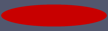
(a)

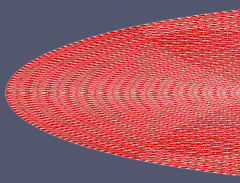
(b)

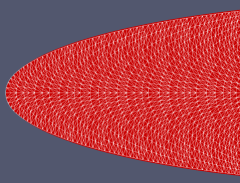
(c)

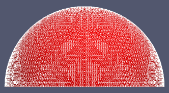
(d)

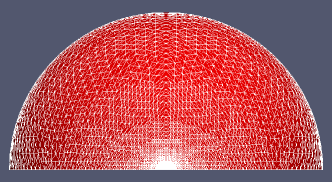
(e)

Figure 2: Improvement of the computational mesh for the stationary domain presented in Figure 2a. The initial mesh is shown in Figure 2b (for $n=6$ initial global mesh refinements). The result of Algorithms 1 and 2 is presented in Figure 2c. In both pictures the red colour indicates the original shape of the domain. Figure 2c indicates that the scheme provides a mesh of high quality with a good approximation of the original shape. The mesh of the reference manifold is presented in 2d and 2e. See Example $1$ for more details.

Figure 3: Mesh qualtity $\sigma_{max}$, see (3.1), for the computational mesh in Figure 2. In the left image the results are shown for $n=5$ and $n=6$ initial global mesh refinements. For $t<0$, the mesh is deformed in order to obtain a bad test mesh. At time $t=0$, this deformation is stopped. For $t>0$, Algorithms 1 and 2 are applied to improve the mesh quality again. The refinement and coarsening strategy in Algorithm 2 can lead to sharp jumps in the mesh quality, see the enlarged section on the right hand side. Since mesh refinement and coarsening is a local procedure, its effect on the mesh quality is corrected very quickly by Algorithm 1. See Example $1$ for more details.

Example 2: Mesh improvement for moving flat domains in $\mathbb{R}^{2}$

We now use Algorithm 1 in order to preserve the mesh quality of a moving domain when the initial mesh is already of high quality.

Example 2.1

We first consider the unit disk $\Gamma(0):=B_{1}(0)\subset\mathbb{R}^{2}$ which is deformed according to (2.1) with

$$v(x_{1},x_{2})=(0.0,-x_{2}(1.0-x_{1}^{2})^{2}+0.2x_{1})^{T}.$$ (4.5)

The computational parameters are $\tau=0.02~{}h_{min}^{2}$, $\alpha=1.0$ and $T_{adapt}=0.01$. The results are presented in Figures 4 and 5.

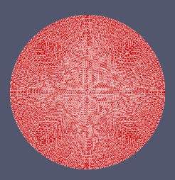
(a)

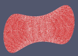
(b)

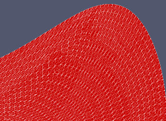
(c)

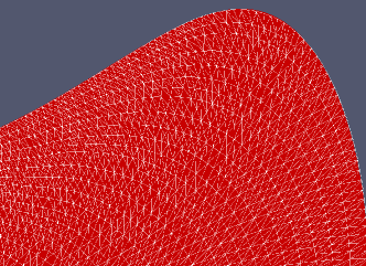
(d)

Figure 4: Comparison of the mesh behaviour for a moving domain in $\mathbb{R}^{2}$. The circular shape in Figure 4a is deformed according to the velocity field $v$ in (4.5) into the domain shown in Figure 4b. An enlarged section of the resulting mesh is presented in Figures 4c and 4d, respectively. If Algorithms 1 and 2 are applied, the mesh quality is not affected by the shape deformation, see Figures 4d and 5. See Example $2.1$ for more details.

Figure 5: Mesh quality $\sigma_{max}$, see (3.1), for the computational mesh in Figure 4. The domain deformation reduces the mesh quality considerably if the mesh vertices are not redistributed. In contrast, the mesh quality remains high if the mesh is moved according to Algorithm 1. See Example $2.1$ for more details.

Example 2.2

In the next example, we consider the domain $\Gamma(t)=B_{r_{1}}(0)\setminus B_{r_{2}}(p(t))\subset\mathbb{R}^{2}$ with the hole $B_{r_{2}}(p(t))$ around the center $p(t)\in\mathbb{R}^{2}$; see Figure 6a. We choose $r_{1}=2.25$ and $r_{2}=0.25$. The evolution of the domain $\Gamma(t)$ is given by the velocity field $v$ solving

$$\Delta v=0,\quad\textnormal{in $\Gamma(t)$},$$

and $v(x_{1},x_{2})=4(-\sin(2\pi t),\cos(2\pi t))^{T}$ on the interior boundary as well as $v(x_{1},x_{2})=0$ on the exterior boundary. In the time interval $[0,1]$, this velocity field induces a circular movement of the hole $B_{r_{2}}(p(t))$ in the interior of the disk $B_{r_{1}}(0)$. The boundary $\partial B_{r_{1}}(0)$ remains unchanged. We approximate the velocity field $v$ by the solution $v_{h}^{m}\in V_{h}(\Gamma_{h}^{m})^{2}$ of

$$\int_{\Gamma_{h}^{m}}\nabla_{\Gamma_{h}^{m}}v_{h}^{m}:\nabla_{\Gamma_{h}^{m}}\varphi_{h}\;do=0,\quad\forall\varphi_{h}\in\overset{\circ}{V}_{h}(\Gamma_{h}^{m})^{2},$$ (4.6)

and $v_{h}^{m}=I_{h}v$ on $\partial\Gamma_{h}^{m}$. Since $\Gamma(t)$ is not simply-connected, we here cannot use the half-sphere as a reference manifold. Instead, we choose the cylinder (4.2). The computational parameters are $\tau=0.001~{}h_{min}^{2}$, $\alpha=0.1$ and $T_{adapt}=10^{-3}$. The results of the simulations with and without redistribution of mesh vertices are shown in Figures 6 and 7. When Algorithm 1 is not applied, the mesh totally degenerates (including mesh entanglements) and hence could not be used to solve a PDE on the moving domain. In contrast, the mesh obtained by our DeTurck scheme preserves its high quality for all time.

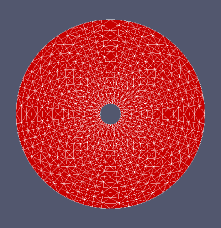
(a)

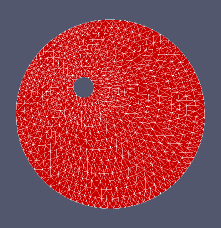
(b)

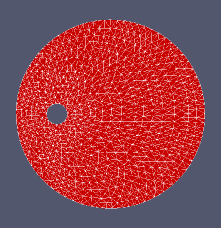
(c)

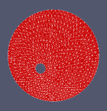
(d)

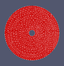
(e)

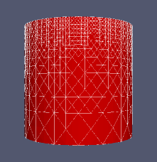
(f)

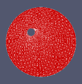
(g)

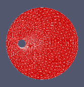
(h)

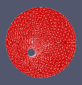
(i)

(j)

Figure 6: Comparison of the mesh behaviour for a moving hole in the interior of the disk $B_{r_{1}}(0)$. The initial mesh is presented in Figure 6a. In this example, the reference manifold is the cylinder (4.2); see Figure 6f for the reference mesh $\mathcal{M}_{h}$ at time $t=1.0$. The local mesh refinement and coarsening of the reference mesh is due to Algorithm 2. Figures 6g to 6j show the time-development of the computational mesh moved according to the velocity field defined in (4.6). This motion leads to the degeneration of the mesh (including mesh entanglements) after a short time. In contrast, our redistribution scheme in Algorithm 1 (together with Algorithm 2) provides a high-quality mesh for all times; see Figures 6b to 6e as well as Figure 7. See Example $2.2$ for more details.

Figure 7: Mesh quality $\sigma_{max}$, see (3.1), for the computational mesh in Figure 6. The computational mesh degenerates after a short time if it is moved according to the velocity field defined in (4.6). The redistribution of the mesh vertices by Algorithm 1 can prevent such mesh degenerations. See Example $2.2$ for more details.

Example 3: Mesh improvement for moving surfaces

Example 3.1

So far, we have only considered flat domains, although within our implementation these domains were treated as hypersurfaces in $\mathbb{R}^{3}$. In this example, we study the behaviour of the DeTurck scheme for a curved surface $\Gamma(t)\subset\mathbb{R}^{3}$ that evolves according to (2.1) with

$$v(x_{1},x_{2},x_{3},t)=(1.5x_{1}x_{3},0.5x_{2}x_{3},r^{2}\sin(4\varphi)\cos(\pi t/2))^{T},$$ (4.7)

where $(r,\varphi)\in[0,\infty)\times[0,2\pi)$ are such that $(x_{1},x_{2})=(r\cos\varphi,r\sin\varphi)$. The initial surface is the unit disk embedded into $\mathbb{R}^{3}$, that is

$$\Gamma(0):=\{x\in\mathbb{R}^{3}\;|\;x_{1}^{2}+x^{2}_{2}\leq 1\;\textnormal{and}\;x_{3}=0\},$$

see Figure 8a. The computational parameters for the simulation are $\tau=0.02~{}h_{min}^{2}$, $\alpha=1.0$ and $T_{adapt}=10^{-3}$. We first observe that the mesh moved according to Algorithm 1 properly approximates the shape of $\Gamma(t)$ on the time interval $[0,0.8]$, see Figures 8a to 8e. In Figure 8 the red area always shows the shape that is computed without the use of Algorithm 1. Furthermore, Figure 9 once again shows that the DeTurck scheme preserves the mesh quality.

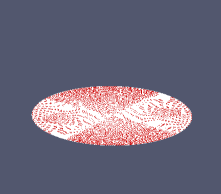
(a)

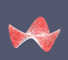
(b)

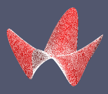
(c)

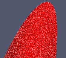
(d)

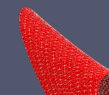
(e)

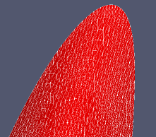
(f)

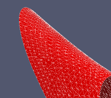
(g)

Figure 8: Comparison of the mesh behaviour for a moving surface in $\mathbb{R}^{3}$. The initial surface is shown in Figure 8a. The surface is deformed according to the velocity field in (4.7). Figures 8b to 8e show the computational mesh obtained by Algorithm 1, while Figures 8f and 8g show the mesh without redistribution of mesh vertices. Figure 9 shows that in Algorithm 1, the mesh quality is not affected by the surface deformation. See Example $3.1$ for more details.

Figure 9: Mesh quality $\sigma_{max}$, see (3.1), for the computational mesh in Figure 8. If Algorithms 1 and 2 are applied, the surface deformation has almost no effect on the quality of the computational mesh in the time interval $[0,0.8]$. See Example $3.1$ for more details.

Example 3.2

So far, we have only used the DeTurck scheme to produce a nice mesh for a moving surface with a known velocity field. We will now demonstrate that the redistribution of the mesh vertices is indeed very useful in order to solve PDEs on evolving surfaces. We will couple the evolution of the surface to a PDE by considering the mean curvature flow, that is $x_{t}=-(H\vec{n})\circ x$. Here, $H:=\nabla_{\Gamma}\cdot\vec{n}$ is the sum of the principal curvatures, that is the mean curvature, and $\vec{n}$ denotes a unit normal to $\Gamma(t)$. Note that the mean curvature flow does not depend on the choice of $\vec{n}$. It is well known, that this evolution equation is equivalent to the heat equation

$$x_{t}=\Delta_{g(t)}x.$$

We will here consider Dirichlet boundary conditions. The initial shape $\Gamma(0):=x_{0}(\mathcal{M})$ is shown in Figure 10a. It can be parametrized by

$$X(r,\varphi)=(r(1+\tfrac{1}{4}\sin(4\varphi))\cos\varphi,r(1+\tfrac{1}{4}\sin(4\varphi))\sin\varphi,\tfrac{1}{4}r^{2}\sin(4\varphi)+\tfrac{3}{4}(1-r^{2}))^{T}$$

with $(r,\varphi)\in[0,1]\times[0,2\pi)$. In order to compute this flow without mesh redistribution, we determine the solutions $u_{h}^{m+1}\in V_{h}(\Gamma_{h}^{m})^{3}$ of

$$\int_{\Gamma_{h}^{m}}\tfrac{1}{\tau}I_{h}(u^{m+1}_{h}\cdot\varphi_{h})+\nabla_{\Gamma_{h}^{m}}u^{m+1}_{h}:\nabla_{\Gamma_{h}^{m}}\varphi_{h}\;do=\int_{\Gamma_{h}^{m}}\tfrac{1}{\tau}I_{h}(\tilde{u}_{h}^{m}\cdot\varphi_{h})\;do$$ (4.8)

for all $\varphi_{h}\in\overset{\circ}{V}_{h}(\Gamma_{h}^{m})^{3}$ with $u_{h}^{m+1}=\tilde{u}_{h}^{m}$ on $\partial\Gamma_{h}^{m}$. This scheme is a variation of the scheme proposed in [10]. For the simulation with DeTurck redistribution, we modify Algorithm 1 in the following way: We replace the first equation in (3.3) by

$$\int_{\Gamma_{h}^{m}}\tfrac{1}{\tau}I_{h}(u^{m+1}_{h}\cdot\varphi_{h})+\nabla_{\Gamma_{h}^{m}}u^{m+1}_{h}:\nabla_{\Gamma_{h}^{m}}\varphi_{h}+\tfrac{1}{\alpha}\sum_{\sigma,\kappa=1}^{3}((\hat{H}^{m}_{h})^{-1}\nabla_{{\Gamma}_{h}^{m}}\hat{y}_{h,\sigma}^{m})_{\kappa}I_{h}\big{(}{\tilde{\zeta}}^{m,\sigma}_{h}\varphi_{h}^{\kappa}\big{)}\;do$$

$$\qquad=\int_{\Gamma_{h}^{m}}\tfrac{1}{\tau}I_{h}(\tilde{u}^{m}_{h}\cdot\varphi_{h})\;do,\quad\forall\varphi_{h}\in\overset{\circ}{V}_{h}({\Gamma}_{h}^{m})^{3}.$$

The second equation in (3.3) is not changed. This is our new DeTurck scheme for the computation of the mean curvature flow with Dirichlet boundary conditions; see also the recent paper [14] on the mean curvature-DeTurck flow on closed manifolds. The parameters used for Figure 10 were $\tau=0.01~{}h_{min}^{2}$, $\alpha=1.0$, and $T_{adapt}=10^{-3}$. The numerical results in Figures 10 and 11 show that without the redistribution of the mesh points the computational mesh totally degenerates. In contrast, the mesh quality under the DeTurck scheme is preserved.

Remark 9.

In the above example, we have considered the motion of a surface with fixed boundary. For this class of problems a variant of the approach presented in this paper might be more suitable. Reparametrizing the evolution equations by solutions to the harmonic map heat flow with Dirichlet boundary conditions seems to be more natural if the boundary is fixed. However, it is not clear whether a scheme based on such a reparametrization is able to preserve the mesh quality in the interior of the surface. This problem has to be studied elsewhere.

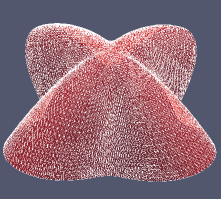
(a)

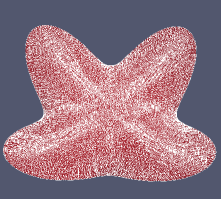
(b)

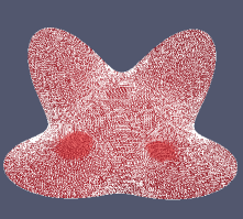
(c)

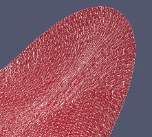
(d)

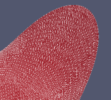
(e)

Figure 10: Comparison of the mesh behaviour for a surface that is deformed according to the mean curvature flow with Dirichlet boundary conditions. The initial surface is presented in Figure 10a. Without redistribution the mesh totally degenerates, see Figures 10b and 10d. By using Algorithms 1 and 2, the mesh remains regular; see Figures 10c and 10e and Figure 11. Note that the DeTurck scheme also leads to a redistribution of the vertices at the boundary of the surface. See Example $3.2$ for more details.

Figure 11: Mesh quality $\sigma_{max}$, see (3.1), for the computational mesh in Figure 10. Without the redistribution of the mesh vertices induced by Algorithm 1 the motion by mean curvature leads to a strong degeneration of the computational mesh. See Example $3.2$ for more details.

Example 4: A free boundary problem: The Hele-Shaw flow coupled to the DeTurck reparametrization

Free and moving boundary problems, [15], provide a wide field of applications in which moving meshes might be useful. A classical well studied problem is that of Hele-Shaw flow, [15, 19, 30]. Let $\Gamma(t)\subset\mathbb{R}^{2}$ be a bounded domain in $\mathbb{R}^{2}$ and $p:\Gamma(t)\rightarrow\mathbb{R}$ the solution to the following boundary value problem

$$\Delta p=\delta_{q},\quad\textnormal{in $\Gamma(t)$,}$$

$$p=\sigma\kappa,\quad\textnormal{on $\partial\Gamma(t)$,}$$

where $\Delta$ denotes the usual Laplacian in $\mathbb{R}^{2}$. $\sigma\in(0,\infty)$ is a surface tension constant and $\kappa$ is the curvature of the free boundary. Here, the curvature $\kappa$ is supposed to be positive when the domain $\Gamma(t)$ is convex. We choose $\Gamma(0)$ to be the unit disk with center $(0.0,-0.5)\in\mathbb{R}^{2}$. There is a sink at the point $q=(0.0,0.0)\in\Gamma(0)$. The co-normal velocity $v_{\partial\Gamma}$ of $\partial\Gamma(t)$ satisfies the kinematic boundary condition

$$v_{\partial\Gamma}=-\tfrac{1}{12}(\nabla_{\nu(t)}p)\nu(t)\quad\textnormal{on $\partial\Gamma(t)$}.$$ (4.9)

In order to obtain a base velocity field $v$ for the parametrization of $\Gamma(t)$, we impose $v=v_{\partial\Gamma}$ on $\partial\Gamma(t)$ and

$$\Delta v=0\quad\textnormal{in $\Gamma(t)$,}$$ (4.10)

instead of taking the physical velocity $-\tfrac{1}{12}\nabla p$ which is singular at the sink. In order to solve the Hele-Shaw flow, we determine the solution $\tilde{p}^{m}_{h}\in V_{h}(\Gamma_{h}^{m})$ of

$$\int_{\Gamma^{m}_{h}}\nabla\tilde{p}^{m}_{h}\cdot\nabla\varphi_{h}\;do=0,\quad\textnormal{$\forall\varphi_{h}\in\overset{\circ}{V}_{h}(\Gamma_{h}^{m})$,}$$

$$\int_{\partial\Gamma^{m}_{h}}I_{h}(\tilde{p}^{m}_{h}\psi_{h})\;do=\sigma\int_{\partial\Gamma^{m}_{h}}\nabla_{\partial\Gamma^{m}_{h}}id_{|\partial\Gamma^{m}_{h}}:\nabla_{\partial\Gamma^{m}_{h}}I_{h}(\nu_{h}^{m}\psi_{h})\;do-\int_{\partial\Gamma^{m}_{h}}\ I_{h}(G_{q}\psi_{h})\;do,$$

for all $\psi_{h}\in V_{h}(\partial\Gamma_{h}^{m})$, where $G_{q}(x)=\tfrac{1}{2\pi}\log(|x-q|)$. The vector field $\nu_{h}^{m}\in V_{h}(\Gamma_{h}^{m})^{n}$ is defined in each vertex $p_{j}\in\partial\Gamma_{h}^{m}$ to be the normalized sum of the two outwards co-normals associated with the two adjacent boundary simplices of $p_{j}$. We compute an approximation $v_{h}^{m}\in V_{h}(\Gamma^{m}_{h})$ to the velocity field $v$ defined in (4.9) and (4.10) by

$$\int_{\Gamma^{m}_{h}}\nabla v^{m}_{h}:\nabla\varphi_{h}\;do=0,\quad\textnormal{$\forall\varphi_{h}\in\overset{\circ}{V}_{h}(\Gamma_{h}^{m})^{n}$,}$$

$$\int_{\partial\Gamma^{m}_{h}}I_{h}(v_{h}^{m}\cdot\psi_{h})\;do=-\tfrac{1}{12}\int_{\partial\Gamma^{m}_{h}}\nabla\tilde{p}^{m}_{h}\cdot I_{h}(\nu^{m}_{h}(\nu_{h}^{m}\cdot\psi_{h}))+I_{h}(\nabla G_{q}\cdot\nu^{m}_{h}(\nu^{m}_{h}\cdot\psi_{h}))\;do,$$

for all $\psi_{h}\in V_{h}(\partial\Gamma_{h}^{m})^{2}$. This gives us a base velocity $v_{h}^{m}$ for the motion of $\Gamma_{h}^{m}$. We use this vector field in (3.3) of Algorithm 1. In Figures 12 and 13 we compare the simulation based on Algorithm 1 to the method when the mesh vertices are just moved by $p_{j}=p_{j}+\tau v_{h}^{m}(p_{j})$. In both approaches we use Algorithm 2 as mesh refinement and coarsening strategy again. The parameters used for the simulation were $\tau=0.005~{}h_{min}^{2}$, $\alpha=1.0$, $T_{adapt}=0.01$ and $\sigma=10^{-3}$.

We observe a far better mesh behaviour of the approach based on the DeTurck reparametrization. Furthermore, the numerical solutions of both approaches strongly differ for times $t\gtrsim 5.0$. Since the solution based on the scheme without DeTurck redistribution has sharp corners at the boundary, it must be rejected. In contrast, the solution obtained by Algorithm 1 satisfies the theoretical expectations – including the formation of a cusp close to the sink.

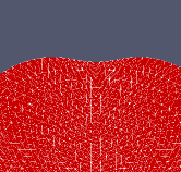
(a)

(b)

(c)

(d)

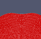
(e)

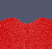
(f)

(g)

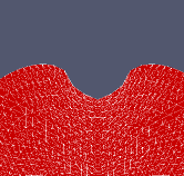
(h)

Figure 12: Comparison of the mesh behaviour for a domain evolving according to the Hele-Shaw flow described in Example $4$. The initial shape is a unit disk. Figures 12e and 12h show the results without redistribution of mesh vertices, whereas in Figures 12a to 12d the application of Algorithm 1 is presented. In Figure 12h the mesh is degenerated (see also Figure 13) and its boundary has sharp corners. This observation suggests that the numerical result in Figure 12d is a much better approximation of the solution to the Hele-Shaw flow at time $t=5.34$. See Example $4$ for more details.

Figure 13: Mesh quality $\sigma_{max}$, see (3.1), for the mesh in Figure 12. Without redistribution of vertices, the mesh degenerates when the domain starts to form a cusp. This suggests that the numerical result in Figures 12a to 12d is a far better approximation to the solution of the Hele-Shaw flow than the result in Figures 12e to 12h. See Example $4$ for more details.

Example 5: The ALE ESFEM and the DeTurck trick for solving PDEs on evolving surfaces

In the last example, we present how the method proposed in this paper can be used in the ALE ESFEM introduced in [16, 17]. We consider the advection-diffusion equation

$$\partial^{\circ}p+p\nabla_{\Gamma(t)}\cdot v-\nabla_{\Gamma(t)}\cdot(D\nabla_{\Gamma(t)}p)=f,\quad\textnormal{in $\Gamma(t)$,}$$ (4.11)

$$\nu(t)\cdot\nabla_{\Gamma(t)}p=0,\quad\textnormal{on $\Gamma(t)$.}$$ (4.12)

Here, $D>0$ denotes a constant scalar diffusivity. $v:\Gamma(t)\rightarrow\mathbb{R}^{n}$ is the velocity field of the medium in which the diffusion process takes place. The medium is supposed to be contained in $\Gamma(t)$. More precisely, we assume that $\Gamma(t)$ also moves with velocity $v$. We here choose $\Gamma(0)=B_{r_{1}}(0)\setminus B_{r_{2}}(0)\subset\mathbb{R}^{2}$ with $r_{1}=2.25$ and $r_{2}=0.25$, and furthermore,

$$v(x_{1},x_{2})=(-7\sin(2\pi t)(1-\tfrac{16}{81}(x_{1}^{2}+x_{2}^{2})),7\cos(2\pi t)(1-\tfrac{16}{81}(x_{1}^{2}+x_{2}^{2})))^{T}$$

for all $(x_{1},x_{2})\in\Gamma(t)$. The material derivative $\partial^{\circ}p$ is defined by

$$(\partial^{\circ}p)\circ x:=\frac{d}{dt}(p\circ x),$$

where $x$ is supposed to be the embedding, whose time derivative is described by $v$; see (2.1). If $p$ is differentiable in an open neighbourhood of $\Gamma(t)\subset\mathbb{R}^{n}$, we obviously obtain

$$\partial^{\circ}p=p_{t}+v\cdot\nabla p.$$

Similarly, the derivative $\partial^{\bullet}$ defined in (2.6) satisfies

$$\partial^{\bullet}p=p_{t}+\hat{v}\cdot\nabla p.$$

Hence, we have

$$\partial^{\circ}p-\partial^{\bullet}p=(v-\hat{v})\cdot\nabla p=(v-\hat{v})\cdot\nabla_{\Gamma(t)}p.$$ (4.13)

Multiplying (4.11) by a test function $\varphi(t)\in H^{1,2}(\Gamma(t))$, integrating and applying the transport formula, see Theorem 5.1 in [11], yields

$$\frac{d}{dt}\int_{\Gamma(t)}p\varphi\;do+D\int_{\Gamma(t)}\nabla_{\Gamma(t)}p\cdot\nabla_{\Gamma(t)}\varphi\;do=\int_{\Gamma(t)}p\partial^{\circ}\varphi+f\varphi\;do,\quad\forall\varphi\in H^{1,2}(\Gamma(t)).$$

Assuming that we only consider test functions $\varphi(t)$ with $\partial^{\bullet}\varphi=0$ and using (4.13), this leads to

$$\frac{d}{dt}\int_{\Gamma(t)}p\varphi\;do+D\int_{\Gamma(t)}\nabla_{\Gamma(t)}p\cdot\nabla_{\Gamma(t)}\varphi\;do=\int_{\Gamma(t)}p(v-\hat{v})\cdot\nabla_{\Gamma(t)}\varphi+f\varphi\;do,\quad\forall\varphi\in H^{1,2}(\Gamma(t)).$$

Motivated by the work in [16], we thus define $p_{h}^{m+1}\in V_{h}(\Gamma_{h}^{m+1})$ to be the solution of

$$\int_{\Gamma^{m+1}_{h}}\tfrac{1}{\tau}I_{h}(p_{h}^{m+1}\varphi^{m+1}_{h})+D\nabla_{\Gamma^{m+1}_{h}}p^{m+1}_{h}\cdot\nabla_{\Gamma^{m+1}_{h}}\varphi_{h}^{m+1}+I_{h}(p_{h}^{m+1}v_{DeT,h}^{m+1,\beta})(\nabla_{\Gamma^{m+1}_{h}}\varphi^{m+1}_{h})_{\beta}\;do$$

$$=\int_{\Gamma^{m}_{h}}\tfrac{1}{\tau}I_{h}(p_{h}^{m}\varphi_{h}^{m})\;do+\int_{\Gamma^{m+1}_{h}}I_{h}(f^{m+1}\varphi_{h}^{m+1})\;do,$$ (4.14)

for all $\varphi_{h}^{m+1}\in V_{h}(\Gamma^{m+1}_{h})$, where $\Gamma^{m+1}_{h}$ is computed according to Algorithm 1 and $\varphi^{m+1}_{h}\in V_{h}(\Gamma^{m+1}_{h})$ is such that it has the same coefficients with respect to the Lagrange basis functions of $V_{h}(\Gamma^{m+1}_{h})$ as $\varphi^{m}_{h}\in V_{h}(\Gamma^{m}_{h})$ has with respect to the Lagrange basis functions of $V_{h}(\Gamma^{m}_{h})$; see [16] for more details. The vector field $v^{m+1}_{DeT,h}\in V_{h}(\Gamma^{m+1}_{h})^{n}$ is defined by $v^{m+1}_{DeT,h}\circ u^{m+1}_{h}:=\tfrac{1}{\tau}(u^{m+1}_{h}-\tilde{u}_{h}^{m})-I_{h}v^{m}$. Here we aim to approximate the solution

$$p(x,t)=\cos(2\pi t)\exp(-|x|^{2})$$ (4.15)

of (4.11) and (4.12) for the right hand side

$$f(x,t)=\left(\cos(2\pi t)(2v_{0}\cdot x-2v\cdot x+4D(1-|x|^{2}))-2\pi\sin(2\pi t)\right)exp(-|x|^{2}),$$

where $v_{0}:=(\tfrac{112}{81}\sin(2\pi t),-\tfrac{112}{81}\cos(2\pi t))^{T}$. The numerical result of (4.14) for the parameters $\tau=0.001~{}h_{min}^{2}$, $\alpha=0.1$, $T_{adapt}=10^{-3}$ and $D=2.0$ is presented in Figure 14.

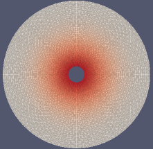
(a)

(b)

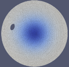
(c)

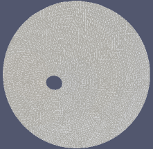
(d)

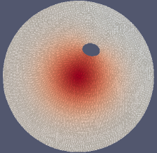
(e)

Figure 14: Numerical approximation of the advection-diffusion equation (4.11) on a moving domain $\Gamma(t)$. The mesh of the domain is deformed according to Algorithms 1 and 2. The numerical solution $p_{h}^{m}$ of (4.14) is indicated by the colour scheme red $\approx 1$, grey $\approx 0$ and blue $\approx-1$. The true solution is given in (4.15). This example demonstrates how Algorithm 1 in combination with the ALE-method in [16] can be used to solve a PDE on a moving submanifold with boundary. For more details see Example $5$.

5 Discussion

We think that the remeshing approach proposed in this paper has the potential to be very useful for many applications with moving boundaries. Since it is based on the discretization of a PDE, it would, in principle, be possible to use standard techniques of Numerical Analysis to estimate discretization errors connected with this method. This is certainly one of the advantages of our approach. In our numerical experiments, we observed that our scheme can improve the mesh quality of a given mesh or preserve the mesh quality for a moving mesh provided that the reference mesh is of sufficiently high quality.

We also observed that Algorithm 1 tends to deform $\Gamma_{h}^{m}$ to a mesh with simplices of different size but similar shape as those of the reference mesh $\mathcal{M}_{h}$. This behaviour is due to the fact that Algorithm 1 is based on the DeTurck trick. Under certain conditions, the harmonic map heat flow converges to a harmonic map as time tends to infinity, see [21]. For a stationary submanifold $\Gamma$ this would mean that the mesh $\Gamma_{h}$ is the image of the reference mesh $\mathcal{M}_{h}$ under an approximation to the inverse of a harmonic map. On the other hand, harmonic maps between compact orientable surfaces are known to be conformal maps under certain conditions, see [13]. It is therefore not surprising that in our experiments the triangles of the computational mesh and of the reference mesh often seem to have similar angles. A side effect of this behaviour is that the area of the simplices of $\Gamma_{h}$ tends to decrease or increase non-homogeneously. The easiest way to take this into account is to apply a refinement and coarsening strategy like in Algorithm 2. Fortunately, as we have seen in Section 4, the mesh quality is not critically affected by the mesh refinement or coarsening – in particular, because the refinement and coarsening procedure only changes the mesh quality locally. Since the time step size $\tau$ of the scheme depends critically on the time scale of the remeshing procedure, that is on $\alpha$, it would be advantageous to have a strategy for finding the optimal parameter $\alpha$. Here, optimal means that $\alpha$ should be as large as possible, since this enables larger time steps $\tau$, and at the same time sufficiently small to ensure a good mesh quality for all times. This issue remains open for future research.

Acknowledgements

The second author would like to thank the Alexander von Humboldt Foundation, Germany, for their financial support by a Feodor Lynen Research Fellowship in collaboration with the University of Warwick, UK.

References

- [1] C. Baker, The mean curvature flow of submanifolds of high codimension, PhD thesis, Australian National University (2010). URL http://www.arxiv.org/abs/1104.4409v1
- [2] A. Bonito, R. Nochetto and M. S. Pauletti, Geometrically consistent mesh modification, SIAM J. Numer. Anal. 48 (2010), 1877–1899.
- [3] C. J. Budd, W. Huang and R. D. Russell, Adaptivity with moving grids, Acta Numerica 18 (2009), 111–241.
- [4] B. Chow, P. Lu and L. Ni, Hamilton’s Ricci Flow, Graduate Studies in Mathematics, AMS Science Press (2006).
- [5] U. Clarenz and G. Dziuk, Numerical methods for conformally parametrized surfaces, CPDw04 - Interphase 2003: Numerical Methods for Free Boundary Problems (2003). http://www.newton.ac.uk/webseminars/pg+ws/2003/cpd/cpdw04/0415/dziuk.
- [6] U. Clarenz, N. Litke and M. Rumpf, Axioms and variational problems in surface parameterization, Computer Aided Geometric Design, 21:727–749 (2004).
- [7] K. Deckelnick, G. Dziuk and C. M. Elliott, Computation of geometric partial differential equations and mean curvature flow, Acta Numerica 14 (2005), 139–232.
- [8] D. M. DeTurck, Deforming metrics in the direction of their Ricci tensor, Journal of Differential Geometry 18 (1983), no. 11, 157–162.
- [9] A. S. Dvinsky Adaptive grid generation from harmonic maps on Riemannian manifolds, J. of Comp. Phys. 95 (1991), 450–476.
- [10] G. Dziuk, An algorithm for evolutionary surfaces, Numerische Mathematik 58, no. 1 (1991), 603–611.
- [11] G. Dziuk and C. M. Elliott, Finite element methods for surface PDEs, Acta Numerica 22 (2013), 289–396.
- [12] J. Eells and J. H. Sampson, Harmonic mappings of Riemannian manifolds, Amer. J. Math. 86 (1964), 109–160.
- [13] J. Eells and J. C. Wood, Restrictions on harmonic maps of surfaces, Topology 15 (1976), 263–266.
- [14] C. M. Elliott and H. Fritz, On Approximations of the Curve Shortening Flow and of the Mean Curvature Flow based on the DeTurck trick, Submitted to IMA Journal of Numerical Analysis (2015).
- [15] C. M. Elliott and J. R. Ockendon, Weak and variational methods for moving boundary problems, Pitman, London 213 pp (1982).
- [16] C. M. Elliott and V. M. Styles, An ALE ESFEM for solving PDEs on evolving surfaces, Milan Journal of Mathematics 80 (2012), 469–501.
- [17] C. M. Elliott and C. Venkataraman, Error analysis for an ALE evolving surface finite element method, Num. Methods for PDEs 31 (2015), 459–499.
- [18] H. Fritz, Isoparametric finite element approximation of Ricci curvature, IMA Journal of Numerical Analysis 33, no. 4 (2013), 1265 – 1290.
- [19] B. Gustaffson and A. Vasil’ev, Conformal and Potential Analysis in Hele-Shaw Cells, ISBN 3-7643-7703-8, Birkhauser Verlag (2006).
- [20] S. Haker, S. Angenent, A. Tannenbaum, R. Kikinis, G. Sapiro and M. Halle, Conformal surface parameterization for texture mapping, IEEE Transactions on Visualization and Computer Graphics, 6(2):181–189 (2000).
- [21] R. S. Hamilton, Harmonic maps of manifolds with boundary, Springer Lecture Notes 471 (1975).
- [22] R. S. Hamilton, Heat equations in geometry, Lecture notes, Hawaii (1989).
- [23] R. S. Hamilton, The formation of singularities in the Ricci flow, Surveys in Differential Geometry 227 (1995), 7–136.
- [24] C.-J. Heine, Curvature reconstruction with linear finite elements, Private communications (2009).
- [25] W. Huang, Practical aspects of formulation and solution of moving mesh partial differential equations, J. of Comp. Phys. 171 (2001), 753–775.
- [26] W. Huang and R. D. Russell, Moving mesh strategy based upon a gradient flow equation for two dimensional problems, SIAM J. Sci. Comput. 20, 3 (1998), 998–1015.
- [27] W. Huang and R. D. Russell, Adaptive Moving Mesh Methods, Applied Mathematical Sciences Volume 174, Springer (2011).
- [28] M. Jin, Y. Wang, S.-T. Yau and X. Gu, Optimal global conformal surface parameterization, In Proceedings of the Conference on Visualization ’04 (2004), 267–274.
- [29] J. Jost, Ein Existenzbeweis für harmonische Abbildungen, die ein Dirichlet-Problem lösen, mittels der Methode des Wärmeflusses, Manuscripta mathematica, Vol. 34 (1981), 17–25.
- [30] E. Kelley and E. J. Hinch, Numerical simulations of sink flow in the Hele-Shaw cell with small surface tension, Euro. J. Applied Math. 8 (1997), 533–550.
- [31] G. Macdonald, J. A. Mackenzie, M. Nolan and R. H. Insall, A Computational Method for the Coupled Solution of Reaction-Diffusion Equations on Evolving Domains and Surfaces: Application to a Model of Cell Migration and Chemotaxis, Strathclyde University, Department of Mathematics and Statistics Research Report Number 6 (2015).
- [32] K. Mikula, M. Remešíková, P. Sarkoci, and D. Ševčovič, Manifold evolution with tangential redistribution of points, SIAM J. Sci. Comput. 36, no. 4 (2014), A1384–A1414.
- [33] A. Schmidt and K. G. Siebert, Design of Adaptive Finite Element Software, Lecture Notes in Computational Science and Engineering 42, Springer (2005).
- [34] J. Steinhilber, Numerical analysis for harmonic maps between hypersurfaces and grid improvement for computational parametric geometric flows, PhD thesis, University of Freiburg (2014). URL http://www.freidok.uni-freiburg.de/volltexte/9537/
- [35] A. M. Winslow Numerical solution of the quasilinear poisson equation in a nonuniform triangle mesh, J. of Comp. Phys. Vol. 1, Issue 2 (1966), 149–172.