Properties of the false vacuum
as the quantum unstable state

Abstract

We analyze properties of unstable vacuum states from the point of view of the quantum theory. In the literature one can find some suggestions that some of false (unstable) vacuum states may survive up to times when their survival probability has a non-exponential form. At asymptotically late times the survival probability as a function of time $t$ has an inverse power–like form. We show that at this time region the energy of the false vacuum states tends to the energy of the true vacuum state as $1/t^{2}$ for $t\to\infty$. This means that the energy density in the unstable vacuum state should have analogous properties and hence the cosmological constant $\Lambda=\Lambda(t)$ too. The conclusion is that $\Lambda$ in the Universe with the unstable vacuum should have a form of the sum of the ”bare” cosmological constant and of the term of a type $1/t^{2}$: $\Lambda(t)\equiv\Lambda_{bare}+d/t^{2}$ (where $\Lambda_{bare}$ is the cosmological constant for the Universe with the true vacuum).

1 Introduction

Broad discussion of the problem of false vacuum began after the publication of pioneer papers by Coleman and his colleagues [1, 2, 3]. The authors of these papers discussed the problem of the stability of a physical system in a state which is not an absolute minimum of its energy density, and which is separated from the minimum by an effective potential barrier. In mentioned papers it was shown that even if the state of the early Universe is too cold to activate a ”thermal” transition (via thermal fluctuations) to the lowest energy (i.e. ”true vacuum”) state, a quantum decay from the false vacuum to the true vacuum may still be possible through a barrier penetration via quantum tunneling. Some time ago it appeared that the problem of the decay of the false vacuum state can have a possible relevance in the process of tunneling among the many vacuum states of the string landscape (a set of vacua in the low energy approximation of string theory). In such cases the scalar field potential driving inflation has a multiple, low–energy minima or ”false vacuua”. In such an situation the absolute minimum of the energy density is the ”true vacuum”.

The problem of tunneling cosmological states was studied in many papers. Part of these studies was focused on analysis of the role of the Standard Model Higgs boson in the inflationary cosmology. Results presented in the pioneering paper [4] show that inflation can be natural consequence of the Standard Model. This idea was analyzed in many papers (see eg. [5, 6, 7, 9]). An application of some results of studies of the tunneling cosmological state to the inflationary cosmology driven by the Higgs boson can be found eg. in [10, 11]. The dependence of the inflationary scenario and the dynamics of the Universe (including the problem of the stability of the Standard Model vacuum) on the mass of the Higgs boson was discussed e.g. in [4, 5, 6, 7, 9, 10, 11]. The discovery of the Higgs–like resonance at 125 — 126 GeV (see, eg., [12, 13, 14, 15]) was also the additional cause of much discussions about the stability of the false vacuum. In [13] assuming the validity of the Standard Model up to Planckian energies it was shown that a Higgs mass $m_{h}<126$ GeV implies that the electroweak vacuum is a metastable state. This means that not only inflationary scenario and dynamics of the early Universe depend on Higgs boson mass but also the stability of the vacuum state of the Universe, which is the Standard Model Higgs vacuum. Thus a discussion of Higgs vacuum stability can not concentrate only on the standard model of elementary particles but must be considered also in a cosmological framework, especially when analyzing the process of tunneling among the many vacuum states of the string landscape.

Krauss and Dent analyzing a false vacuum decay [16, 17] pointed out that in eternal inflation, many false vacuum regions can survive up to the times much later than times when the exponential decay law holds. This effect has a simple explanation: It may occur even though regions of false vacua by assumption should decay exponentially, gravitational effects force space in a region that has not decayed yet to grow exponentially fast.

The aim of this talk is to discuss properties of the false vacuum state as an unstable state, and to analyze the late time behavior of the energy of the false vacuum states.

2 Briefly about quantum unstable states

If $|M\rangle$ is an initial unstable state then the survival probability, ${\cal P}(t)$, equals ${\cal P}(t)=|a(t)|^{2}$, where $a(t)$ is the survival amplitude, $a(t)=\langle M|M;t\rangle$, $a(0)=1$, and, $|M;t\rangle=\exp\,[-itH]\,|M\rangle$, $H$ is the total Hamiltonian of the system under considerations. (We use $\hbar=c=1$ units). The spectrum, $\sigma(H)$, of $H$ is assumed to be bounded from below, $\sigma(H)=[E_{min},\infty)$ and $E_{min}>-\infty$.

From basic principles of quantum theory it is known that the amplitude $a(t)$, and thus the decay law ${\cal P}(t)$ of the unstable state $|M\rangle$, are completely determined by the density of the energy distribution function $\omega({\cal E})$ for the system in this state

$$a(t)=\int_{Spec.(H)}\omega({E})\;e^{\textstyle{-\,i\,{E}\,t}}\,d{E},$$ (1)

where $\omega({E})\geq 0\;\;{\rm for}\;\;E\geq E_{min}\;\;{\rm and}\;\;\;\;\omega({E})=0\;\;\;{\rm for}\;\;\;E<E_{min}$. From this last condition and from the Paley–Wiener Theorem it follows that there must be [18] $|a(t)|\;\geq\;A\,\exp\,[-b\,t^{q}]$ for $|t|\rightarrow\infty$. Here $A>0,\,b>0$ and $0<q<1$. This means that the decay law ${\cal P}(t)$ of unstable states decaying in the vacuum can not be described by an exponential function of time $t$ if time $t$ is suitably long, $t\rightarrow\infty$, and that for these lengths of time ${\cal P}(t)$ tends to zero as $t\rightarrow\infty$ more slowly than any exponential function of $t$. The analysis of the models of the decay processes shows that ${\cal P}(t)\simeq\exp\,[-{\it\Gamma}_{M}^{0}t]$, (where ${\it\Gamma}_{M}^{0}$ is the decay rate of the state $|M\rangle$), to a very high accuracy at the canonical decay times $t$: From $t$ suitably later than the initial instant $t_{0}$ up to $t\gg\tau_{M}=1/{{\it\Gamma}_{M}^{0}}$, ($\tau_{M}$ is a lifetime), and smaller than $t=T$, where $T$ is the crossover time and it denotes the time $t$ for which the non–exponential deviations of $a(t)$ begin to dominate.

In general, in the case of quasi–stationary (metastable) states it is convenient to express $a(t)$ in the following form: $a(t)=a_{c}(t)+a_{lt}(t)$, where $a_{c}(t)$ is the exponential (canonical) part of $a(t)$, that is $a_{c}(t)\stackrel{{\scriptstyle\rm def}}{{=}}N\,\exp\,[-it(E_{M}^{0}-\frac{i}{2}\,{\it\Gamma}_{M}^{0})]$, ($E_{M}^{0}$ is the energy of the system in the state $|M\rangle$ measured at the canonical decay times, $N$ is the normalization constant), and $a_{lt}(t)$ is the non–exponential late time part of $a(t)$). For times $t\sim\tau_{M}$: $|a_{c}(t)|\gg|a_{lt}(t)|$. The crossover time $T$ can be found by solving the following equation,

$$|a_{c}(t)|^{\,2}=|a_{lt}(t)|^{\,2}.$$ (2)

The amplitude $a_{lt}(t)$ exhibits inverse power–law behavior at the late time region: $t\gg T$. The integral representation (1) of $a(t)$ means that $a(t)$ is the Fourier transform of the energy distribution function $\omega(E)$. Using this fact we can find asymptotic form of $a(t)$ for $t\rightarrow\infty$. Results are rigorous [19, 20]. If to assume that

$$\omega({E})=({E}-{E}_{min})^{\lambda}\;\eta({E})\;\in\;L_{1}(-\infty,\infty),$$ (3)

(where $0\leq\lambda<1$), and $\eta(E_{min})\stackrel{{\scriptstyle\rm def}}{{=}}\eta_{0}>0$, and $\eta^{(k)}({E})=\frac{d}{dE}\,\eta(E)$, ($k=0,1,\ldots,n$), exist and they are continuous in $[{E}_{min},\infty)$, and limits $\lim_{E\rightarrow{E}_{min}+}\;\eta^{(k)}(E)\stackrel{{\scriptstyle\rm def}}{{=}}\eta_{0}^{(k)}$ exist, and $\lim_{{E}\rightarrow\infty}\;({E}-{E}_{min})^{\lambda}\,\eta^{(k)}({E})=0$ for all above mentioned $k$, then one finds that [19],

$$a(t) \begin{array}[]{c}{}\hfil\\ \sim\\ \scriptstyle{t\rightarrow\infty}\end{array} (-1)\,e^{\textstyle{-{i}{E}_{min}t}}\;\Big{[}\Big{(}-\frac{i}{t}\Big{)}^{\lambda+1}\;\Gamma(\lambda+1)\;\eta_{0}\;$$

$$+\;\lambda\,\Big{(}-\frac{i}{t}\Big{)}^{\lambda+2}\;\Gamma(\lambda+2)\;\eta_{0}^{(1)}\;+\;\ldots\Big{]}=a_{lt}(t),$$

where $\Gamma(x)$ is Euler’s gamma function.

From (2) it is seen that asymptotically late time behavior of the survival amplitude $a(t)$ depends rather weakly on a specific form of the energy density $\omega(E)$. The same concerns a decay curves ${\cal P}(t)=|a(t)|^{2}$. A typical form of a decay curve, that is the dependence on time $t$ of ${\cal P}(t)$ when $t$ varies from $t=t_{0}=0$ up to $t\,>\,30\,\tau_{M}$ is presented in Panels ${\bf\it A}$ of Figs. 1 and 2. Results presented in these Figures were obtained for the Breit–Wigner energy distribution function, $\omega({E})\equiv\omega_{BW}=\frac{N}{2\pi}\,{\it\Theta}(E-E_{min})\ \frac{{\it\Gamma}_{M}^{0}}{({E}-{E}^{0}_{M})^{2}+({\it\Gamma}_{M}^{0}/{2})^{2}}$, which corresponds with $\lambda=0$ in (3).

3 Instantaneous energy of the system in the unstable state

The amplitude $a(t)$ contains information about the decay law ${\cal P}(t)$ of the state $|M\rangle$, that is about the decay rate ${\it\Gamma}_{M}^{0}$ of this state, as well as the energy ${E}_{M}^{0}$ of the system in this state. This information can be extracted from $a(t)$. Indeed if $|M\rangle$ is an unstable (a quasi–stationary) state then $a(t)\cong N\exp\,[-{i}({E}_{M}^{0}-\frac{i}{2}{\it\Gamma}_{M}^{0})\,t]\,=\,a_{c}(t)$ for $t\sim\tau_{M}$. So, there is

$${E}_{M}^{0}-\frac{i}{2}{\it\Gamma}_{M}^{0}\equiv i\,\frac{\partial a_{c}(t)}{\partial t}\;\frac{1}{a_{c}(t)},\;\;(t\sim\tau_{M}),$$ (8)

in the case of quasi–stationary states.

The standard interpretation and understanding of the quantum theory and the related construction of our measuring devices are such that detecting the energy ${E}_{M}^{0}$ and decay rate ${\it\Gamma}_{M}^{0}$ one is sure that the amplitude $a(t)$ has the canonical form $a_{c}(t)$ and thus that the relation (8) occurs. Taking the above into account one can define the ”effective Hamiltonian”, $h_{M}$, for the one–dimensional subspace of states ${\cal H}_{||}$ spanned by the normalized vector $|M\rangle$ as follows [19, 20, 21]

$$h_{M}\stackrel{{\scriptstyle\rm def}}{{=}}i\,\frac{\partial a(t)}{\partial t}\;\frac{1}{a(t)}\;\stackrel{{\scriptstyle\rm def}}{{=}}{\cal E}_{M}(t)\,-\,\frac{i}{2}\,\gamma_{M}(t).$$ (9)

In general, $h_{M}$ can depend on time $t$, $h_{M}\equiv h_{M}(t)$. One meets this effective Hamiltonian when one starts with the Schrödinger Equation for the total state space ${\cal H}$ and looks for the rigorous evolution equation for the distinguished subspace of states ${\cal H}_{||}\subset{\cal H}$ (see Appendix and also [19, 20]). Using $h_{M}(t)$ one finds the following expressions for the energy and the decay rate of the system in the state $|M\rangle$ under considerations, to be more precise for the instantaneous energy ${\cal E}_{M}(t)$ and the instantaneous decay rate, $\gamma_{M}(t)$ (see Appendix and [19]),

$${\cal E}_{M}\equiv{\cal E}_{M}(t)=\Re\,[h_{M}(t)],\;\;\;\;\;\gamma_{M}\equiv\gamma_{M}(t)=-\,2\,\Im\,[h_{M}(t)],$$ (10)

where $\Re\,(z)$ and $\Im\,(z)$ denote the real and imaginary parts of $z$ respectively.

Defining

$$h_{M}^{lt}(t)\stackrel{{\scriptstyle\rm def}}{{=}}{h_{M}(t)\vline}_{\,t\rightarrow\infty}$$ (11)

one can calculate the asymptotic late time form $h_{M}^{lt}(t)$ of $h_{M}(t)$ using asymptotic late time form of the amplitude $a_{lt}$(t):

$$h_{M}^{lt}(t)=i\,\frac{\partial a_{lt}(t)}{\partial t}\;\frac{1}{a_{lt}(t)}.$$ (12)

So, starting from the asymptotic expression (2) for $a(t)$ and using (12) one can find $h_{M}^{lt}(t)$ for times $t\gg T$ as a function of a small parameter $x=1/t$: $h_{M}^{lt}(x)=\frac{b(x)}{a_{lt}(x)}$, where $b(x)=i{\frac{\partial a_{lt}(t)}{\partial t}\vline}_{x=\frac{1}{t}}$, then expanding such obtained $h_{M}^{lt}(x)$ in Taylor series about $x=0$ one obtains after some algebra that

$${h_{M}(t)\vline}_{\,t\rightarrow\infty}=h_{M}^{lt}(t)\simeq{E}_{min}+(-\,\frac{i}{t})\,c_{1}\,+\,(-\,\frac{i}{t})^{2}\,c_{2}\,+\,\ldots,$$ (13)

where $c_{i}=c_{i}^{\ast},\;\;i=1,2,\ldots$; (coefficients $c_{i}$ depend on $\omega(E)$). This last relation means that

$${\cal E}_{M}(t)\,\simeq\,E_{min}\,-\,\frac{c_{2}}{t^{2}}\ldots,\;\;\;\;\;\;\;\gamma_{M}(t)\,\simeq\,2\,\frac{c_{1}}{t}\,+\ldots,\;\;\;({\rm for}\;\;t\gg T).$$ (14)

These properties take place for all unstable states which survived up to times $t\gg T$. Note that from (14) it follows that $\lim_{t\rightarrow\infty}\,{\cal E}_{M}(t)=E_{min}$ and $\lim_{t\rightarrow\infty}\,\gamma_{M}(t)=0$.

For the density $\omega(E)$ of the form (3) (i. e. for $a(t)$ having the asymptotic form given by (2)) we have

$$c_{1}=\lambda+1,\;\;\;\;c_{2}=(\lambda+1)\,\frac{\eta^{(1)}(E_{min})}{\eta(E_{min})}.$$ (15)

The energy distribution densities $\omega(E)$ considered in quantum mechanics and in quantum field theory can be described by $\omega(E)$ of the form (3), eg. quantum field theory models analyzing two particle decays correspond with $\lambda=\frac{1}{2}$.

A general form of

$$\kappa(t)=\frac{{\cal E}_{M}(t)-E_{min}}{E_{M}^{0}-E_{min}},$$ (16)

as a function of time $t$ varying from $t=t_{0}=0$ up to $t>T$ is presented in Panels ${\bf\it B}$ of Figs. 1 and 2. These results were obtained for $\omega(E)=\omega_{BW}(E)$. The crossover time $T$, that is the time region where fluctuations of ${\cal P}(t)$ and ${\cal E}_{M}(t)$ take place depends on the value of the parameter $s_{0}=(E_{M}^{0}-E_{min})/{\it\Gamma}_{M}^{0}$ in the model considered: The smaller $s_{0}$ the shorter $T$.

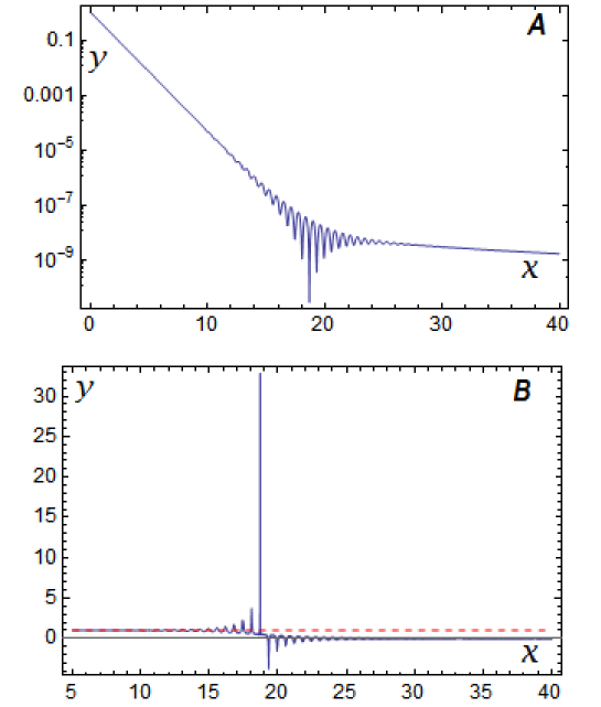
Figure 1: The case $s_{0}=10$. Panel ${\bf\it A}$ — Axes: $y={\cal P}(t)$, (The logarithmic scale), $x=t/\tau_{M}$. Panel ${\bf\it B}$, Axes: $y=\kappa(t)$, $x=t/\tau_{M}$. The horizontal red dashed line denotes $y=\kappa(t)=1$.

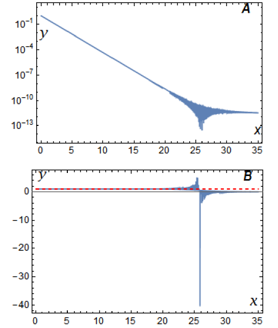
Figure 2: The case $s_{0}=50$. Panel ${\bf\it A}$ — Axes: $y={\cal P}(t)$, (The logarithmic scale), $x=t/\tau_{M}$. Panel ${\bf\it B}$, Axes: $y=\kappa(t)$, $x=t/\tau_{M}$. The horizontal red dashed line denotes $y=\kappa(t)=1$, that is ${\cal E}_{M}(t)=E_{M}^{0}$.

The equivalent formula for $h_{M}(t)$ is given by the following relation:

$$h_{M}(t)\equiv\frac{\langle M|H|M(t)\rangle}{\langle M|M(t)\rangle}.$$ (17)

This last relation explains properties of ${\cal E}_{M}(t)$ at different time regions which one can see in Panels $B$ of Figs. 1 and 2. Indeed, if to rewrite the numerator of the righthand side of (17) as follows,

$$\langle M|H|M(t)\rangle\equiv\langle M|H|M\rangle\,a(t)\,+\,\langle M|H|M(t)\rangle_{\perp},$$ (18)

where $|M(t)\rangle_{\perp}=Q|M(t)\rangle$, $Q=\mathbb{I}-P$ is the projector onto the subspace od decay products, $P=|M\rangle\langle M|$ and $\langle M|M(t)\rangle_{\perp}=0$, then one can see that there is a permanent contribution of decay products described by $|M(t)\rangle_{\perp}$ to the energy of the unstable state considered. The intensity of this contribution depends on time $t$. This contribution into the instantaneous energy is practically negligible small and constant in time at canonical decay times whereas at the transition times, when $t\sim T$, it is fluctuating function of time and the amplitude of these fluctuations may be significant. What is more relations (17) and (18) allow one to proof that in the case of unstable states $\Re\,[h_{M}(t)]\neq const$. Using these relations one obtains that

$$h_{M}(t)=E_{M}+\,\frac{\langle M|H|M(t)\rangle_{\perp}}{a(t)},$$ (19)

where $E_{M}$ is the expectation value of $H$: $E_{M}=\langle M|H|M\rangle$. From this relation one can see that $h_{M}(0)=E_{M}$ if the matrix elements $\langle M|H|M\rangle$ exists. It is because $|M(t=0)\rangle_{\perp}=0$ and $a(t=0)=1$. Now if to assume that for $0\leq t_{1}\neq t_{2}$ there is $\Re\,[h_{M}(0)]=\Re\,[h_{M}(t_{1})]=\Re\,[h_{M}(t_{2})]=const$ then one immediately conclude that there should be $\Re\,[h_{M}(t)]=E_{M}$ for any $t\geq 0$. Unfortunately such an observation contradicts implications of (19): From this relation it follows that $\Re\,[\frac{\langle M|H|M(t)\rangle_{\perp}}{a(t)}]\neq 0$ for $t>0$ and thus $\Re\,[h_{M}(t>0)]\neq E_{M}\equiv\Re\,[h_{M}(0)]$ which shows that $\Re\,[h_{M}(t)]\equiv{\cal E}_{M}(t)$ can not be constant in time.

4 Connections with the cosmology

From the point of the quantum theory the decay of the false vacuum is the quantum decay process [1, 2, 3, 16, 17]. What is more some cosmological scenario predict the possibility of decay of the Standard Model vacuum at an inflationary stage of the evolution of the universe (see eg. [22] and also [8] and reference therein). Of course this decaying Standard Model vacuum is described by the quantum state corresponding to a local minimum of the energy density which is not the absolute minimum of the energy density of the system considered. This means that state vector corresponding to the false vacuum is a quantum unstable (or metastable) state. Therefore all the general properties of quantum unstable states must also occur in the case of such a quantum unstable state as false vacuum. This applies in particular to such properties as late time deviations from the exponential decay law and properties of the energy ${\cal E}^{false}_{0}(t)$ of the system in the quantum false vacuum state at late times $t>T$.

The cosmological scenario in which false vacuum may decay at the inflationary stage of the universe corresponds with the hypothesis analyzed by Krauss and Dent in [16]. Namely in the mentioned paper the hypothesis that some false vacuum regions do survive well up to the time $T$ or later was formulated. So, let $|M\rangle=|0\rangle^{false}$, be a false, $|0\rangle^{true}$ – a true, vacuum states and $E^{false}_{0}$ be the energy of a state corresponding to the false vacuum measured at the canonical decay time and $E^{true}_{0}$ be the energy of true vacuum (i.e. the true ground state of the system). As it is seen from the results presented in previous Section, the problem is that the energy of those false vacuum regions which survived up to $T$ and much later differs from $E^{false}_{0}$ [23].

Now, if one assumes that $E^{true}_{0}\equiv E_{min}$ and $E_{0}^{false}=E_{M}^{0}$ and takes into account results of the previous Section (including those in Panels $\bf\it B$ of Figs. 1 and 2) then one can conclude that the energy of the system in the false vacuum state has the following general properties:

$${\cal E}^{false}_{0}(t)=E^{true}_{0}+\Delta E\;\cdot\;\kappa(t),$$ (20)

where $\Delta E=E_{0}^{false}\,-\,E^{true}_{0}$ and $\kappa(t)\simeq 1$ for $t\sim\tau_{0}^{false}<T$, (where $\tau_{0}^{false}$ is the life time of the unstable false vacuum state). $\kappa(t)$ is a fluctuating function of $t$ at $t\sim T$ and $\kappa(t)\propto\frac{1}{t^{2}}$ for $t\gg T$.

At asymptotically late times, $t\gg T$, one finds that

$${\cal E}^{false}_{0}(t)\simeq E^{true}_{0}-\frac{c_{2}}{t^{2}}\ldots\;\;\neq\,E^{false}_{0},$$ (21)

where $c_{2}=c_{2}^{\ast}$ and it can be positive or negative depending on the model considered. Similarly $\gamma^{false}_{0}(t)\simeq+2\,c_{1}/t\,\ldots$ for $t\gg T$. Two last properties of the false vacuum states mean that

$${\cal E}^{false}_{0}(t)\rightarrow E^{true}_{0}\;\;{\rm and}\;\;\gamma^{false}_{0}(t)\rightarrow 0\;\;{\rm as}\;\;t\rightarrow\infty.$$ (22)

Now if one wants to generalize the above results obtained on the basis of quantum mechanics to quantum field theory one should take into account among others a volume factors so that survival probabilities per unit volume per unit time should be considered. The standard false vacuum decay calculations shows that the same volume factors should appear in both early and late time decay rate estimations (see Krauss and Dent [16, 24]). This means that the calculations of cross–over time $T$ can be applied to survival probabilities per unit volume. For the same reasons within the quantum field theory the quantity ${\cal E}_{M}(t)$ can be replaced by the energy per unit volume $\rho_{M}(t)={\cal E}_{M}(t)/V$ because these volume factors $V$ appear in the numerator and denominator of the formula (9) for $h_{M}(t)$. This conclusion seems to hold when considering the energy ${\cal E}_{0}^{false}(t)$ of the system in false vacuum state $|0\rangle^{false}$ because Universe is assumed to be homogeneous and isotropic at suitably large scales. So at such scales to a sufficiently good accuracy we can extract properties of the energy density $\rho_{0}^{false}=E_{M}^{0}/V=E_{0}^{false}/V$ of the system in the false vacuum state $|0\rangle^{false}$ from properties of the energy ${\cal E}_{0}^{false}(t)$ of the system in this state defining $\rho_{0}^{false}(t)$ as $\rho_{0}^{false}(t)={\cal E}_{0}^{false}(t)/V$. This means that in the case of a meta–stable (unstable or decaying, false) vacuum the following important property of $\kappa(t)$ holds:

$$\kappa(t) \equiv \frac{\rho_{0}^{false}(t)-\rho_{bare}}{\rho_{0}^{false}-\rho_{bare}},$$

where $\rho_{bare}=E_{min}/V$ is the energy density of the true (bare) vacuum. From the last equation the following relation follows

$$\rho_{0}^{false}(t)-\rho_{bare}=(\rho_{0}^{false}-\rho_{bare})\,\kappa(t).$$

Thus, because for $t<T$ there is $\kappa(t)\simeq 1$, one finds that

$$\rho_{0}^{false}(t)\simeq\rho_{0}^{false},\;\;{\rm for}\;\;t<T,$$

whereas for $t\gg T$ we have

$$\rho_{0}^{false}(t)-\rho_{bare}=(\rho_{0}^{false}-\rho_{bare})\,\kappa(t)\simeq\pm\,d_{2}\,\frac{\hbar^{2}}{t^{2}},\;\;(t\gg T),$$ (23)

where $d_{2}=d_{2}^{\ast}$. The units $\hbar=1=c$ will be used in the next formulas. Analogous relations (with the same $\kappa(t))$ take place for $\Lambda(t)=\frac{8\pi G}{c^{2}}\,\rho(t)$, or $\Lambda(t)=8\pi G\,\rho(t)$ in $\hbar=c=1$ units:

$$\Lambda(t)-\Lambda_{bare}=(\Lambda_{0}-\Lambda_{bare})\,\kappa(t),$$ (24)

or,

$$\Lambda(t)=\Lambda_{bare}+(\Lambda_{0}-\Lambda_{bare})\,\kappa(t).$$ (25)

One may expect that $\Lambda_{0}$ equals to the cosmological constant calculated within quantum field theory. From (25) it is seen that for $t<T$,

$$\Lambda(t)\simeq\Lambda_{0},\;\;\;{\rm for}\;\;\;(t<T),$$ (26)

because $\kappa(t<T)\simeq 1$. Now if to assume that $\Lambda_{0}$ corresponds to the value of the cosmological ”constant” $\Lambda$ calculated within the quantum field theory, than one should expect that [25]

$$\frac{\Lambda_{o}}{\Lambda_{bare}}\geq 10^{120},$$ (27)

which allows one to write down Eq. (25) as follows

$$\Lambda(t)\simeq\Lambda_{bare}+\Lambda_{0}\,\kappa(t).$$ (28)

Note that for $t\gg T$ there should be (see (23))

$$\Lambda_{0}\,\kappa(t)\simeq{8\pi G}\,\frac{d_{2}}{t^{2}}\equiv\pm\frac{\alpha^{2}}{t^{2}},\;\;{\rm for}\;\;(t\gg T).$$ (29)

5 Final Remarks

Parametrization following from quantum theoretical treatment of metastable vacuum states can explain why the cosmologies with the time–dependent cosmological constant $\Lambda(t)$ should be considered. Such a parametrization may help to explain the cosmological constant problem [26, 27]. From the literature we know that the time dependence of $\Lambda$ of the type $\Lambda(t)=\Lambda_{bare}+\frac{\alpha^{2}}{t^{2}}$ was considered by many authors: Similar form of $\Lambda$ was obtained in [28], where the invariance under scale transformations of the generalized Einstein equations was studied. Such a time dependence of $\Lambda$ was postulated also in [29] as the result of the analysis of the large numbers hypothesis. The cosmological model with time dependent $\Lambda$ of the above postulated form was studied also in [30]. This form of $\Lambda$ was assumed in eg. in [31] but there was no any explanation what physics suggests such the choice. Cosmological model with time dependent $\Lambda$ were also studied in much more recent papers.

The advantage of the formalism presented in Sect. 4 is that it takes into account that the decay proces of the metastable vacuum state is the quantum decay process. So in the case of the universe with metastable (false) vacuum when one realizes that the decay of this unstable vacuum state is the quantum decay process then it emerges automatically that there have to exist the true ground state of the system that is the true (or bare) vacuum with the minimal energy, $E_{min}>-\infty$, of the system corresponding to him and equivalently, $\rho_{bare}=E_{min}/V$, or $\Lambda_{bare}$. Also in this case such $\Lambda\equiv\Lambda(t)$ emerges that at suitable late times it has the form described by relations (28), (29). In such a case the function $\kappa(t)$ given by the relation (16) describes time dependence for all times $t$ of the energy density $\rho_{M}(t)$ or the cosmological ”constant” $\Lambda_{M}(t)$ and it general form is presented in Panels $\bf\it B$ in Figs. 1 and 2. Note that results presented in Sections 2 — 4 are rigorous. The formalism mentioned was applied in [24, 25], where cosmological models with $\Lambda(t)=\Lambda_{bare}\pm\frac{\alpha^{2}}{t^{2}}$ were studied: The nice and may be the most promising result is reported in [25] where using the parametrization following from the mentioned quantum theoretical analysis of the decay process of the unstable vacuum state an attempt was made to explain the small today’s value of the cosmological constant $\Lambda$. So we can conclude that formalism and the approach described in this paper and in [24, 25] is promising and can help to solve the cosmological constant and other cosmological problems and it needs further studies. What is more, in the light of the LHC result concerning the mass $m_{H}$ of the Higgs boson and cosmological consequences of this result such conclusions seem to be reasonable and justified. It is because according to the observation that result $m_{H}<126$ GeV may impliy instability of the electroweak vacuum and that there are cosmological scenario that predict even the possibility of decay of this vacuum at an inflationary stage of the evolution of the universe [8, 22].

Acknowledgments: The work was supported in part by the NCN grant No DEC-2013/09/B/ST2/03455.

Appendix

Let us consider general properties of $h_{M}(t)$. In the proper quantum mechanical calculations of the decay processes one always starts from the Schrödinger equation

$$i\frac{\partial}{\partial t}|M(t)\rangle=H|M(t)\rangle.$$ (30)

Here $|M(t)\rangle\in{\cal H}$, $H$ denotes the total self–adjoint Hamiltonian and $|M\rangle=|M(0)\rangle\in{\cal H}$ is the initial unstable state of the system. There is $\langle M|M\rangle=1$. To be more precisely the problem reduces to replacing Schrödinger equation (30) by two coupled equations and then by solving them to obtain the equation for the amplitude $a(t)$. Using projection operators defined in Sec. 3, $P=|M\rangle\langle M|$ and $Q=\mathbb{I}-P$ one can see that simply

$$P|M;t\rangle\equiv a(t)\,|M\rangle,$$ (31)

and instead of (30) one obtains two coupled equations (see eg. [32])

$$i\,\frac{\partial}{\partial t}\,P|M(t)\rangle = PHP|M(t)\rangle+PHQ|M(t)\rangle,$$ (32)

$$i\,\frac{\partial}{\partial t}Q|M(t)\rangle = QHQ|M(t)\rangle+QHP|M(t)\rangle.$$ (33)

The initial conditions are:

$$P|M(0)\rangle=|M\rangle,\;\;\;\;Q|M(0)\rangle=0.$$ (34)

Taking into account initial conditions (34) and inserting a solution $Q|M(t)\rangle$ of Eq. (33) into Eq. (32) one obtains the equation for the amplitude $a(t)$:

$$\Big{(}i\frac{\partial}{\partial t}-PHP\Big{)}\,a(t)\,|M\rangle=-i\int_{0}^{\infty}\,k(t-\tau)\,a(\tau)\,|M\rangle\,d\tau,$$ (35)

where $t\geq 0$, and

$$k(t)=\Theta(t)\,\langle M|HQ\,e^{\textstyle{-itQHQ}}\,QH|M\rangle,$$ (36)

($\Theta(t)$ is a unit step function). There is

$$PHP\equiv\langle M|H|M\rangle\,|M\rangle\equiv E_{M}\,|M\rangle,$$

where $E_{M}$. This last property means that Eq. (35) can be rewritten as follows (see [32] or [33] where similar, equivalent equations were considered),

$$\Big{(}i\frac{\partial}{\partial t}-E_{M}\Big{)}\,a(t)=-i\int_{0}^{\infty}\,k(t-\tau)\,a(\tau)\,d\tau.$$ (37)

Equations (35) and (37) are exact. Performing calculations of decay processes one usually uses approximate methods to solve (37). In order to obtain corrections to the energy of the unstable states it is convenient to replace integro–differential equation (37) by equivalent, only differential one:

$$\Big{(}i\frac{\partial}{\partial t}-E_{M}\,-\,v_{M}(t)\Big{)}\,a(t)\equiv 0,$$ (38)

where the ”quasi–potential” $v_{M}(t)$ can be found by solving the non–linear equation:

$$v_{M}(t)\,a(t)=-i\int_{0}^{\infty}\,k(t-\tau)\,a(\tau)\,d\tau.$$ (39)

The approximate solution of this equation to lowest nontrivial order can be found using the ”free” solution $a^{(0)}(t)$ of (37), that is using solutions of the following equation

$$\Big{(}i\frac{\partial}{\partial t}-E_{M}\Big{)}\,a^{(0)}(t)=0,$$ (40)

for the initial condition $a^{(0)}(0)=a(0)=1$. Inserting solution $a^{(0)}(t)=\exp\,[-itE_{M}]$ of (40) into (39) one obtains (for details see [32], Eq. (32) — (35)),

$$v_{M}(t)\simeq v_{M}^{(1)}(t)=-i\int_{0}^{\infty}\,k(t-\tau)\,e^{\textstyle{i(t-\tau)E_{M}}}\,d\tau.$$ (41)

This relation leads to the following expression for $v_{M}^{(1)}(t)$:

$$v_{M}^{(1)}(t)=\langle M|HQ\,\frac{e^{\textstyle{-it(QHQ-E_{M})}}\,-\,1}{QHQ\,-\,E_{M}}\,HQ|M\rangle\equiv-\Delta^{(1)}_{M}(t)-\frac{i}{2}\,{\it\Gamma}^{(1)}_{M}(t),$$ (42)

where $\Delta^{(1)}_{M}(t)$ and ${\it\Gamma}^{(1)}_{M}(t)$ are real. For large $t$ this approximate result coincides with the Weisskopf–Wigner result [34, 32]:

$$\lim_{t\to\infty}\,v_{M}^{(1)}(t)=v_{M}^{(1)}=-\Delta^{(1)}_{M}-\frac{i}{2}{\it\Gamma}^{(1)}_{M},$$ (43)

where

$$\Delta^{(1)}_{M}=\langle M|HQ\;\,{\rm P}_{v}\,\frac{1}{QHQ-E_{M}}\;\,QH|M\rangle,$$ (44)

(here ${\rm P}_{v}$ denotes principal value), and $\Delta^{(1)}_{M}$ is the correction to the energy of unstable state, and

$${\it\Gamma}^{(1)}_{M}=2\pi\langle M|HQ\,\delta(QHQ-E_{M})\,QH|M\rangle,$$ (45)

is the decay width. More detailed considerations show that these approximate results describe behavior of the unstable $|M\rangle$ accurate enough only for canonical decay times (i.e. when the exponential decay law holds with sufficient accuracy [18] ).

Taking into account relations (38), (42), (43) and (44) we conclude that the energy $E_{M}^{0}$ of an unstable state $|M\rangle$ at canonical decay times equals

$$E_{M}^{0}\simeq E_{M}-\Delta^{(1)}_{M}\equiv E_{M}+\Re\,[v_{M}^{(1)}].$$ (46)

On the other hand from (38) it follows that

$$E_{M}+v_{M}(t)\equiv\frac{i}{a(t)}\;\frac{\partial a(t)}{\partial t}.$$ (47)

This relation together with (9) means that simply

$$h_{M}(t)\equiv E_{M}+v_{M}(t),$$ (48)

and Eq. (38) can be written as

$$\Big{(}i\frac{\partial}{\partial t}\,-\,h_{M}(t)\Big{)}\,a(t)\equiv 0,$$ (49)

where simply $h_{M}(t)$ is the effective hamiltonian governing time e volution of the unstable state considered. Comparing (48) and (19) one finds that equivalently

$$v_{M}(t)\equiv\frac{\langle M|H|M(t)\rangle_{\perp}}{a(t)}.$$ (50)

From the above analysis it is seen that

$$v_{M}(t=0)=0,$$ (51)

which means that $\Re\,[h_{M}(t=0)]=E_{M}$.

At canonical decay times, we have

$$\Re\,[h_{M}(t)] = E^{0}_{M}\simeq E_{M}-\Delta^{(1)}_{M},\;\;\;({\rm for}\;\;t\sim\tau_{M}),$$ (52)

$$\Im\,[h_{M}(t)] = -\,\frac{1}{2}\,{\it\Gamma}_{M}^{\,0}\simeq-\,\frac{1}{2}\,{{\it\Gamma}}^{(1)}_{M},\;\;\;({\rm for}\;\;t\sim\tau_{M}).$$ (53)

Therefore when one measures the energy of the unstable state considered at canonical decay times, that is at times $t\sim\tau_{M}$ then one expects to obtain the energy $E_{M}^{0}$ defined by formula (52) as the result of the measurement.

So, as it follows from relations (46) — (52) the energy of the system in the unstable state $|M\rangle$, ${\cal E}_{M}(t)$ is equal to the real part of the effective hamiltonian $h_{M}(t)$:

$${\cal E}_{M}(t)=\Re\,[h_{M}(t)]=E_{M}-\Delta_{M}(t),$$ (54)

where $\Delta_{M}(t)\stackrel{{\scriptstyle\rm def}}{{=}}\Re\,[v_{m}(t)]$ and $\Delta_{M}(0)=0$ and the sign of $\Delta_{M}(t)$ depends on the model considered. Strictly speaking, if to take into account all properties of $\Re\,[h_{M}(t)]$, the energy ${\cal E}_{M}(t)$ is the instantaneous energy of the system in the unstable state $|M\rangle$ and this energy is equal to the sum of the expectation value, $E_{M}$ of the total Hamiltonian and the contribution $\Delta_{M}(t)$ coming from the interactions responsible for decay and regeneration processes. To complete the above considerations one should mention connections of late time properties of $v_{M}(t)$ with similar properties of ${\cal E}_{M}(t)$ and $\gamma_{M}(t)$ that have been discussed in Sec. 3. There is at late times $t\gg T$:

$$\Delta_{M}(t)\equiv\Re\,[v_{M}(t)]\simeq E_{M}-E_{min}+\frac{c_{2}}{t^{2}}.....,{\rm for}\;\;t\gg T.$$ (55)

The late time asymptotic form of $\Im\,[v_{M}(t)]\equiv\Im\,[h_{M}(t)]$ coincides with the late time form of $\gamma_{M}(t)$ specified by the formula (14).

References

- [1] S. Coleman, Phys. Rev. D 15, 2929 (1977).
- [2] C.G. Callan and S. Coleman, Phys. Rev. D 16, 1762 (1977).
- [3] S. Coleman and F. de Lucia, —em Phys. Rev. D 21, 3305 (1980).
- [4] F. Bezrukov, M. Shaposhnikov, Phys. Lett. B 659, 703, (2008); arXiv: 0710.3755 [hep–th].
- [5] F. Bezrukov, et al., Phys. Lett. B 675, 88, (2009).
- [6] F. Bezrukov, et al., JHEP 10, 140, (2012); arXiv: 1205.283 [hep–ph].
- [7] A. O. Barvinsky, et al, JCAP, 2008, 0811 (2008) 021; arXiv: 0809.2104 [hep–ph].
- [8] F. Bezrukov, M. Shaposhnikov, Comptes Rendus Physique, 16, 994, (2015).
- [9] A. O. Barvinsky, em et al, Eur. Phys. J. C (2012) 72:2219; arXiv: 0910.1041 [hep–ph].
- [10] A. O. Barvinsky et al, Phys. Rev. D 81, 0435530, (2010).
- [11] A. O. Barvinsky, Theoret. Math. Phys. 170, 52, (2012).
- [12] A. Kobakhidze, A. Spencer–Smith, Phys. Lett. B 722, 130,(2013).
- [13] G. Degrassi, et al., JHEP 1208, 098, (2012).
- [14] J. Elias–Miro, et al., Phys. Lett. B 709, 222, (2012).
- [15] Wei Chao, et al., Phys. Rev. D 86, 113017, (2012).
- [16] L. M. Krauss, J. Dent, Phys. Rev. Lett., 100, 171301 (2008).
- [17] S. Winitzki, Phys. Rev. D 77, 063508 (2008).
- [18] L. A. Khalfin, Zh. Eksp. Teor. Fiz. 33, 1371 (1957); [Sov. Phys. JETP 6, 1053 (1958)].
- [19] K. Urbanowski, Eur. Phys. J. D, 54, 25, (2009).
- [20] K. Urbanowski, Cent. Eur. J. Phys. 7, 696 (2009).
- [21] F. Giraldi, Eur. Phys. J., D 69: 5 (2015).
- [22] V. Branchina, E. Messina, Phys. Rev. Lett., 111, 241801, (2013).
- [23] K. Urbanowski, Phys. Rev. Lett., 107, 209001 (2011).
- [24] K. Urbanowski, M. Szyd owski, AIP Conf. Proc. 1514, 143 (2013); doi: 10.1063/1.4791743.
- [25] M. Szydłowski, Phys. Rev. D 91, 123538 (2015).
- [26] S. Weinberg, Rev. Mod. Phys. 61, 1 (1989).
- [27] S. M. Carroll, The Cosmological Constant, Living Rev. Relativity, 3, (2001), 1; http://www.livingreviews.org/lrr-2001-1.
- [28] V. Canuto and S. H. Hsieh, Phys. Rev. Lett. 39, 429, (1977).
- [29] Y. K. Lau and S. J. Prokhovnik, Aust. J. Phys., 39, 339, (1986).
- [30] M. S. Berman, Phys. Rev. D 43, 1075, (1991).
- [31] J. L. Lopez and D. V. Nanopoulos, Mod. Phys. Lett. A 11, 1 (1996).
- [32] K. Urbanowski, Phys. Rev. A 50, 2847, (1994).
- [33] A. Peres, Ann. Phys., 129, 33, (1980).
- [34] V. F. Weisskopf, E. T. Wigner, Z. Phys. 63, 54, (1930); 65, 18, (1930).