Unbiased pseudo-$C_{\ell}$ power spectrum estimation with mode projection

Abstract

With the steadily improving sensitivity afforded by current and future galaxy surveys, a robust extraction of two-point correlation function measurements may become increasingly hampered by the presence of astrophysical foregrounds or observational systematics. The concept of mode projection has been introduced as a means to remove contaminants for which it is possible to construct a spatial map reflecting the expected signal contribution. Owing to its computational efficiency compared to minimum-variance methods, the sub-optimal pseudo-$C_{\ell}$ (PCL) power spectrum estimator is a popular tool for the analysis of high-resolution data sets. Here, we integrate mode projection into the framework of PCL power spectrum estimation. In contrast to results obtained with optimal estimators, we show that the uncorrected projection of template maps leads to biased power spectra. Based on analytical calculations, we find exact closed-form expressions for the expectation value of the bias and demonstrate that they can be recast in a form that allows a numerically efficient evaluation, preserving the favorable ${{\cal O}\!\left(\ell_{\mathrm{max}}^{3}\right)}$ time complexity of PCL estimator algorithms. Using simulated data sets, we assess the scaling of the bias with various analysis parameters and demonstrate that it can be reliably removed. We conclude that in combination with mode projection, PCL estimators allow for a fast and robust computation of power spectra in the presence of systematic effects – properties in high demand for the analysis of ongoing and future large scale structure surveys.

1 Introduction

In modern cosmology, measurements of the power spectrum (or its real-space counterpart, the angular correlation function) have proven a powerful summary statistic and are widely used to confront theoretical models with observational data, e.g., Smoot et al. (1992); Hancock et al. (1994); Gundersen et al. (1995); Netterfield et al. (1997); Hanany et al. (2000); Halverson et al. (2002); Kovac et al. (2002); Hinshaw et al. (2003); Fowler et al. (2010); Lueker et al. (2010); Planck Collaboration et al. (2014); The Polarbear Collaboration: P. A. R. Ade et al. (2014); BICEP2/Keck and Planck Collaborations et al. (2015) for an arbitrary selection of measurements of the cosmic microwave background radiation (CMB) two-point correlation function, or, e.g., Totsuji & Kihara (1969); Hermit et al. (1996); Norberg et al. (2001); Blake & Wall (2002); Zehavi et al. (2002); Tegmark et al. (2004); Croom et al. (2005); Eisenstein et al. (2005); Coil et al. (2008); Reid et al. (2010); Beutler et al. (2011); Kim et al. (2014); Crocce et al. (2016) for constraints on galaxy clustering.

A decrease in statistical errors resulting from the increasing coverage or sensitivity of ongoing and future experiments will impose stricter limits on the level of contamination of the targeted cosmological signal by secondary sources. Such contaminants may be of astrophysical origin (e.g., foreground emission or dust extinction, e.g., Maller et al. 2005) or the result of complications associated with the data collection and processing procedure (for example, survey depth fluctuations, varying seeing conditions, image calibration uncertainties, Huterer et al. 2013; Awan et al. 2016). To aid assessment of the possible impact of systematic effects that may have altered the observed signal, it has become standard for galaxy surveys to compile libraries of template maps that describe the spatial variation of survey properties (Scranton et al., 2002; Ross et al., 2011, 2012; Leistedt & Peiris, 2014; Leistedt et al., 2016; Ross et al., 2016). Several approaches have been proposed that make use of these maps to correct measurements of the two-point statistics for systematic effects (Rybicki & Press 1992; Ho et al. 2012; Leistedt & Peiris 2014, see Elsner et al. 2016 for a comparison). In Kalus et al. (2016), the authors derive a template cleaning procedure for the popular FKP estimator (Feldman et al., 1994).

In the following, we focus on the mode projection procedure of Rybicki & Press (1992). Attributing infinite variance to modes described by a set of templates, specific signal patterns can be excluded from the analysis and the computed result hence becomes more robust with respect to systematics captured by them (see, e.g., Tegmark et al., 1998; Slosar et al., 2004; Smith et al., 2009; Elsner & Wandelt, 2013; Leistedt et al., 2013, for applications). Unfortunately, mode projection can only be straightforwardly implemented in case the estimator makes use of inverse variance-weighted data. Within the field of power spectrum estimation, this is the case for the maximum likelihood estimator (Bond et al., 1998) and the optimal quadratic estimator (Tegmark, 1997). Regrettably, both of them are very expensive to evaluate numerically, usually prohibitively so for state-of-the-art high-resolution data (Borrill, 1999). Conversely, the much faster pseudo-$C_{\ell}$ (PCL) estimator introduced by Hivon et al. (2002) makes no attempt at exact inverse variance-weighting, trading optimality for computational speed, and can be applied in only ${{\cal O}\!\left(\ell_{\mathrm{max}}^{3}\right)}$ time to a data set band-limited at multipole moment $\ell_{\mathrm{max}}$. The purpose of this paper is to demonstrate that the concept of mode projection can be successfully integrated into the framework of PCL estimators, combining the desirable properties of fast and robust power spectrum estimation.

This article is organized as follows. In Sect. 2, we review the concept of mode projection and discuss how it can be implemented in PCL estimators. Then, we use numerical simulations to verify our results and systematically study the impact of mode projection for different analysis parameters (Sect. 3). We conclude by summarizing our findings in Sect. 4.

2 PCL mode projection

We start this section by providing a detailed review of mode projection (Rybicki & Press, 1992). Straightforwardly integrated into optimal power spectrum estimators, it was shown to lead to unbiased results at the cost of an increase in the estimator variance that is modest compared to other systematics mitigation schemes (Elsner et al., 2016).

We first consider a contaminant that can be described by a single non-vanishing template $f$ and contributes with unknown scalar amplitude $\epsilon$ to the data vector $d$,

$$d=s+\epsilon f\,.$$ (1)

Even if the simple linear model in Eq. (1) is not fully appropriate, we can still use it as a first order approximation of a Taylor expansion in $f$ for small values of $\epsilon$. In the following, we assume the absence of correlations between stochastic signal realizations $s$ and the deterministic template $f$ used in the projection in the ensemble average.

Then, our goal is to find a means to infer the power spectrum of the targeted cosmological signal $s$,

$$\widehat{C}_{\ell{}}^{\,\mathrm{s}}=\sum_{m}\frac{1}{2\ell+1}\left|s_{\ell{}m{}}\right|^{2}\,,$$ (2)

where we have introduced the “hat” notation to specify an estimated quantity for a specific realization of the analyzed field.

In case an analysis is based on inverse variance-weighted data only, mode projection is implemented by modifying the data covariance matrix $\bm{C}$. A rank-one term, constructed from the template, is added with variance $\sigma$. Afterwards, we take the limit to assign infinite variance to this specific signal direction,

$$\bm{\widetilde{C}}=\lim_{\sigma\to\infty}\left(\bm{C}+\sigma ff^{\dagger}\right)\,.$$ (3)

Then, any analysis making use of the data $d$ in form of

$$\widetilde{d}=\bm{\widetilde{C}}^{-1}d$$ (4)

will be insensitive to a contaminant described by the template.

Guided by Eqs. (3) and (4), we now implement mode projection within the framework of pseudo-$C_{\ell}$ power spectrum estimation. Since PCL does not make use of inverse variance-weighted maps, we apply the PCL estimator to a filtered version of the data. The filter is linear and can be expressed in terms of a matrix,

$$\bm{F}=\lim_{\sigma\to\infty}\left(\mathbb{1}+\sigma ff^{\dagger}\right)^{-1}\,,$$ (5)

where $\mathbb{1}$ is the identity matrix. Making use of the Sherman-Morrison formula, we can take the limit and find an exact expression for the filter,

$$\bm{F}=\mathbb{1}-\frac{ff^{\dagger}}{f^{\dagger}f}\,.$$ (6)

We therefore derive for the preprocessed data vector $\widetilde{d}=\bm{F}d$,

$$\widetilde{d}=d-\frac{f^{\dagger}d}{f^{\dagger}f}\,f\,.$$ (7)

From Eq. (7) the well known equivalence between mode projection and a direct subtraction becomes apparent again (Rybicki & Press, 1992), i.e., the data are cleaned by removing a template contribution with amplitude estimate $\hat{\epsilon}=\left.f^{\dagger}d\middle/f^{\dagger}f\right.$.

As a side note, we mention that Eq. (7) represents the simplest case where all modes are assigned equal weights in the calculation of the cleaning coefficient $\hat{\epsilon}$. Relaxing this assumption would require introducing a weight matrix $\bm{W}$ such that $\hat{\epsilon}=\left.f^{\dagger}\bm{W}d\middle/f^{\dagger}\bm{W}f\right.$. For $\bm{W}=\bm{C}^{-1}$, we then recover the maximum likelihood cleaning approach that is implicitly used in optimal mode projection algorithms. Since it is possible to construct the Cholesky decomposition $\bm{W}=\bm{U}^{\dagger}\bm{U}$ for any given positive-definite weight matrix, we can choose to consider the prewhitened data vector $d_{\mathrm{w}}=\bm{U}d$ instead, and absorb all remaining factors of $\bm{U}$ by redefining $f_{\mathrm{w}}=\bm{U}f$, leading back to Eq. (7). We can therefore set the weight matrix to unity in what follows.

As we will demonstrate below, even in the absence of any contaminant, applying a power spectrum estimator to $\widetilde{d}$ to measure the statistical properties of $s$ will in general lead to biased results. We now derive analytical expressions for the expectation value of the bias introduced by mode projection. We begin our discussion by analyzing the simplest possible case, the projection of a single template on the full sky, and then gradually generalize our findings to take into account the effects of multiple templates and limited sky coverage. Readers only interested in our main result may skip the first paragraphs and continue with Sect. 2.4. In our calculation, we will assume that the Fourier modes of the field analyzed are mutually uncorrelated to sufficient precision in the ensemble average, i.e., $\langle s_{\ell{}m{}}\ s_{\ell{{}^{\prime}}m{{}^{\prime}}}^{\ast}\rangle\propto\delta_{\ell\ell^{\prime}}\delta_{mm^{\prime}}$.

2.1 Full sky analysis, single template

We start out considering a full sky analysis where a single template has been projected out. Given the filtered data map Eq. (7) as input, we derive the mean variance of its spherical harmonic coefficients,

$$\langle\widetilde{d}_{\ell{}m{}}\ \widetilde{d}_{\ell{}m{}}^{\ast}\rangle=\langle s_{\ell{}m{}}\ s_{\ell{}m{}}^{\ast}\rangle-\frac{2}{f^{\dagger}f}\langle s_{\ell{}m{}}\ (s^{\dagger}f)f_{\ell{}m{}}^{\ast}\rangle\\ +\frac{1}{\left(f^{\dagger}f\right)^{2}}\langle(f^{\dagger}s)f_{\ell{}m{}}\ (s^{\dagger}f)f_{\ell{}m{}}^{\ast}\rangle\,.$$ (8)

Denoting the power spectrum of the template realization used in the projection as $\widehat{C}_{\ell{}}^{\,\mathrm{f}}$, we obtain for the normalization factor in the above expression

$$f^{\dagger}f=\sum_{\ell}(2{\ell{}}+1)\widehat{C}_{\ell{}}^{\,\mathrm{f}}\,,$$ (9)

a measure of the total variance of $f$. Introducing further $C_{\ell{}}^{\,\mathrm{s}}=\langle\widehat{C}_{\ell{}}^{\,\mathrm{s}}\rangle$ as the ensemble averaged signal power spectrum, we derive the following expectation values for the multipole moments $(\ell,m)$,

$$\langle s_{\ell{}m{}}\ (s^{\dagger}f)f_{\ell{}m{}}^{\ast}\rangle=C_{\ell{}}^{\,\mathrm{s}}\widehat{C}_{\ell{}}^{\,\mathrm{f}}\,,$$ (10)

$$\langle(f^{\dagger}s)f_{\ell{}m{}}\ (s^{\dagger}f)f_{\ell{}m{}}^{\ast}\rangle=\left(\sum_{\ell^{\prime}}(2{\ell{{}^{\prime}}}+1)C_{\ell{{}^{\prime}}}^{\,\mathrm{s}}\widehat{C}_{\ell{{}^{\prime}}}^{\,\mathrm{f}}\right)\widehat{C}_{\ell{}}^{\,\mathrm{f}}\,.$$ (11)

Projecting a single template on the full sky, the ensemble averaged power spectrum of the filtered data set $\widetilde{d}$ becomes

$$\langle\widehat{C}_{\ell{}}^{\,\mathrm{\widetilde{d}}}\rangle =\sum_{m}\frac{1}{2\ell+1}\langle\widetilde{d}_{\ell{}m{}}\ \widetilde{d}_{\ell{}m{}}^{\ast}\rangle$$

$$=C_{\ell{}}^{\,\mathrm{s}}+b_{\ell}\,.$$ (12)

Since we want to use $\widehat{C}_{\ell{}}^{\,\mathrm{\widetilde{d}}}$ as a proxy for the signal power spectrum $\widehat{C}_{\ell{}}^{\,\mathrm{s}}$, we conclude that this estimate is biased. The bias $b_{\ell}$ is given by

$$b_{\ell}=-\frac{2C_{\ell{}}^{\,\mathrm{s}}\widehat{C}_{\ell{}}^{\,\mathrm{f}}}{\sum_{\ell^{\prime}}(2{\ell{{}^{\prime}}}+1)\widehat{C}_{\ell{{}^{\prime}}}^{\,\mathrm{f}}}+\frac{\left(\sum_{\ell^{\prime}}(2{\ell{{}^{\prime}}}+1)C_{\ell{{}^{\prime}}}^{\,\mathrm{s}}\widehat{C}_{\ell{{}^{\prime}}}^{\,\mathrm{f}}\right)\widehat{C}_{\ell{}}^{\,\mathrm{f}}}{\left(\sum_{\ell^{\prime}}(2{\ell{{}^{\prime}}}+1)\widehat{C}_{\ell{{}^{\prime}}}^{\,\mathrm{f}}\right)^{2}}\,.$$ (13)

We therefore obtain a simple recipe to combine mode projection and PCL power spectrum estimation. Instead of directly analyzing a given data set, we first apply a filter function according to Eq. (7). After the power spectrum has been computed, the result is then corrected by subtracting a bias term,

$$\widehat{C}_{\ell{}}^{\,\mathrm{s}}=\widehat{C}_{\ell{}}^{\,\mathrm{\widetilde{d}}}-b_{\ell}\,,$$ (14)

leading to clustering estimates of the signal that are unbiased in the ensemble average and have been marginalized over contaminants described by the template.

An additional complication in the evaluation of Eq. (14) arises from the fact that the bias term in itself is a function of the signal power spectrum. In the full-sky case, it is still feasible to compute $\widehat{C}_{\ell{}}^{\,\mathrm{s}}$ directly by finding the solution to the matrix equation

$$\widehat{C}_{\ell{}}^{\,\mathrm{s}}=\sum_{\ell^{\prime}}\left[\left(\mathbb{1}+B\right)^{-1}\right]_{\ell\ell^{\prime}}\widehat{C}_{\ell{{}^{\prime}}}^{\,\mathrm{\widetilde{d}}}\,,$$ (15)

where

$$B_{\ell_{1}\ell_{2}}=-\frac{2\widehat{C}_{\ell{{}_{1}}}^{\,\mathrm{f}}}{\sum_{\ell^{\prime}}(2{\ell{{}^{\prime}}}+1)\widehat{C}_{\ell{{}^{\prime}}}^{\,\mathrm{f}}}\cdot\delta_{\ell_{1}\ell_{2}}+\frac{(2{\ell{{}_{2}}}+1)\widehat{C}_{\ell{{}_{2}}}^{\,\mathrm{f}}\widehat{C}_{\ell{{}_{1}}}^{\,\mathrm{f}}}{\left(\sum_{\ell^{\prime}}(2{\ell{{}^{\prime}}}+1)\widehat{C}_{\ell{{}^{\prime}}}^{\,\mathrm{f}}\right)^{2}}\,.$$ (16)

It is interesting to note that even though we compute power spectra on the full sky, $B$ will in general contain off-diagonal entries. We conclude that applying the filter Eq. (7) can lead to the coupling of previously uncorrelated Fourier modes. This behaviour is in line with the interpretation that mode projection is equivalent to masking (see Appendix A for a detailed discussion).

We will later see that it is not always possible to find an explicit expression for Eq. (16). In practice, it may therefore be most viable to debias the result iteratively, or, assuming a prior power spectrum for $C_{\ell{}}^{\,\mathrm{s}}$.

2.2 Full sky analysis, multiple templates

To be able to handle multiple (not necessarily linearly independent) templates requires a generalization of the filter matrix used to prepare the data. For a data vector with $n_{\mathrm{pix}}$ elements, we modify Eq. (6) to take a $n_{\mathrm{pix}}\times n_{\mathrm{temp}}$ object $\bm{f}$ as input, containing a collection of $n_{\mathrm{temp}}$ templates,

$$\bm{F}=\mathbb{1}-\bm{f}\left(\bm{f}^{\dagger}\bm{f}\right)^{-1}\bm{f}^{\dagger}\,,$$ (17)

where the normalization factor now becomes a $n_{\mathrm{temp}}\times n_{\mathrm{temp}}$ matrix with entries computed from template auto- and cross-power spectra,

$$\left(\bm{f}^{\dagger}\bm{f}\right)_{ij}=\sum_{\ell}\,(2{\ell{}}+1)\widehat{C}_{\ell{}}^{\,\mathrm{f^{i}\times f^{j}}}\,.$$ (18)

We propose to use the Moore-Penrose inverse for $\left(\bm{f}^{\dagger}\bm{f}\right)^{-1}$ in case this matrix is rank deficient.

Projecting multiple templates on the full sky, Eq. (8) now takes the form

$$\langle\widetilde{d}_{\ell{}m{}}\ \widetilde{d}_{\ell{}m{}}^{\ast}\rangle=\langle s_{\ell{}m{}}\ s_{\ell{}m{}}^{\ast}\rangle-2\sum_{ij}\left(\bm{f}^{\dagger}\bm{f}\right)^{-1}_{ij}\langle s_{\ell{}m{}}\ (s^{\dagger}f^{j})f_{\ell{}m{}}^{i\,\ast}\rangle\\ +\sum_{\begin{subarray}{c}ij\\ hk\end{subarray}}\left(\bm{f}^{\dagger}\bm{f}\right)^{-1}_{ij}\left(\bm{f}^{\dagger}\bm{f}\right)^{-1}_{hk}\langle(f^{j\,\dagger}s)f_{\ell{}m{}}^{i}\ (s^{\dagger}f^{k})f_{\ell{}m{}}^{h\,\ast}\rangle\,,$$ (19)

and we find for the bias

$$b_{\ell}=-2\sum_{ij}\left(\bm{f}^{\dagger}\bm{f}\right)^{-1}_{ij}C_{\ell{}}^{\,\mathrm{s}}\widehat{C}_{\ell{}}^{\,\mathrm{f^{j}\times f^{i}}}+\sum_{\begin{subarray}{c}ij\\ hk\end{subarray}}\left(\bm{f}^{\dagger}\bm{f}\right)^{-1}_{ij}\left(\bm{f}^{\dagger}\bm{f}\right)^{-1}_{hk}\\ \times\left(\sum_{\ell^{\prime}}(2{\ell{{}^{\prime}}}+1)C_{\ell{{}^{\prime}}}^{\,\mathrm{s}}\widehat{C}_{\ell{{}^{\prime}}}^{\,\mathrm{f^{j}\times f^{k}}}\right)\widehat{C}_{\ell{}}^{\,\mathrm{f^{i}\times f^{h}}}\,,$$ (20)

the generalization of Eq. (13) to multiple templates. With this result, we can trivially provide an explicit expression for the generalized bias matrix Eq. (16) that can be used with Eq. (15) to obtain unbiased signal power spectrum estimates,

$$B_{\ell_{1}\ell_{2}}=-2\sum_{ij}\left(\bm{f}^{\dagger}\bm{f}\right)^{-1}_{ij}\widehat{C}_{\ell{{}_{1}}}^{\,\mathrm{f^{j}\times f^{i}}}\cdot\delta_{\ell_{1}\ell_{2}}\\ +\sum_{\begin{subarray}{c}ij\\ hk\end{subarray}}\left(\bm{f}^{\dagger}\bm{f}\right)^{-1}_{ij}\left(\bm{f}^{\dagger}\bm{f}\right)^{-1}_{hk}(2{\ell{{}_{2}}}+1)\widehat{C}_{\ell{{}_{2}}}^{\,\mathrm{f^{j}\times f^{k}}}\widehat{C}_{\ell{{}_{1}}}^{\,\mathrm{f^{i}\times f^{h}}}\,.$$ (21)

2.3 Cut-sky analysis, single template

We now turn to the more realistic case of a cut-sky analysis. To allow a transparent discussion of the problems associated with this complication, we again start by first considering the projection of a single template before generalizing our results later on.

Denoting $a^{\mathrm{full}}_{\ell{}m{}}$ as the spherical harmonics of a field on the full sky, a modified set of coefficients $a^{\mathrm{cut}}_{\ell{}m{}}$ is then obtained by multiplying its real space representation with a non-negative mask $W$,

$$a^{\mathrm{cut}}_{\ell{}m{}} =\sum_{\ell^{\prime}m^{\prime}}a^{\mathrm{full}}_{\ell{{}^{\prime}}m{{}^{\prime}}}\int\mathrm{d}\bm{n}\,Y_{\ell^{\prime}m^{\prime}}(\bm{n})\,W(\bm{n})\,Y_{\ell m}^{\ast}(\bm{n})$$

$$=\sum_{\ell^{\prime}m^{\prime}}a^{\mathrm{full}}_{\ell{{}^{\prime}}m{{}^{\prime}}}K_{\ell m\ell^{\prime}m^{\prime}}\,.$$ (22)

Here, the coupling kernels $K$ capture how the orthogonality relation of the spherical harmonics is modified by the mask. We give their exact definition in Appendix B (Eq. (41)).

A pseudo-$C_{\ell}$ power spectrum estimation algorithm then makes use of the properties of the coupling kernels to obtain a simplified expression that relates power spectra on the full sky to cut-sky spectra with correct properties in the ensemble average,

$$\langle\widehat{C}_{\ell{}}^{\,\mathrm{full}}\rangle=\sum_{\ell^{\prime}}M^{-1}_{\ell\ell^{\prime}}\langle\widehat{C}_{\ell{{}^{\prime}}}^{\,\mathrm{cut}}\rangle\,,$$ (23)

where we have assumed that the inverse of the coupling matrix $M$ exists, a function of the mask power spectrum only (see Eq. (42) for a formal definition).

Based on the framework developed for PCL estimators, it is now possible to compute the mode projection bias (Eq. (13)) for limited sky coverage. In this case, data and template maps are both multiplied with the mask prior to the analysis. We find the expression of the normalization factor Eq. (9) to be unchanged, although it is now calculated from cut-sky template pseudo-power spectra that have not been corrected for the reduced sky fraction. Computing the remaining terms, however, is more complicated. We now obtain (cf. Eqs. (10) and (11)),

$$\langle s_{\ell{}m{}}\ (s^{\dagger}f)f_{\ell{}m{}}^{\ast}\rangle =\sum_{\begin{subarray}{c}\ell_{1,2,3,4}\\ m_{1,2,3,4}\end{subarray}}\!C_{\ell{{}_{2}}}^{\,\mathrm{s}}\ f_{\ell{{}_{1}}m{{}_{1}}}\,f_{\ell{}m{}}^{\ast}\ w_{\ell{{}_{3}}m{{}_{3}}}\,w_{\ell{{}_{4}}m{{}_{4}}}^{\ast}$$

$$\times\sqrt{(2\ell+1)(2\ell_{1}+1)(2\ell_{3}+1)(2\ell_{4}+1)}$$

$$\times\frac{2\ell_{2}+1}{4\pi}\begin{pmatrix}\ell&\ell_{2}&\ell_{3}\\ 0&0&0\end{pmatrix}\begin{pmatrix}\ell_{1}&\ell_{2}&\ell_{4}\\ 0&0&0\end{pmatrix}$$

$$\times\begin{pmatrix}\ell&\ell_{2}&\ell_{3}\\ m&-m_{2}&m_{3}\end{pmatrix}\begin{pmatrix}\ell_{1}&\ell_{2}&\ell_{4}\\ m_{1}&-m_{2}&m_{4}\end{pmatrix}\,,$$ (24)

where the last four objects are Wigner 3j symbols, and

$$\langle(f^{\dagger}s)f_{\ell{}m{}} \ (s^{\dagger}f)f_{\ell{}m{}}^{\ast}\rangle$$

$$=\sum_{\begin{subarray}{c}\ell_{1,2,3,4,5}\\ m_{1,2,3,4,5}\end{subarray}}\!C_{\ell{{}_{3}}}^{\,\mathrm{s}}\ f_{\ell{}m{}}\,f_{\ell{}m{}}^{\ast}\ f_{\ell{{}_{2}}m{{}_{2}}}\,f_{\ell{{}_{1}}m{{}_{1}}}^{\ast}\ w_{\ell{{}_{4}}m{{}_{4}}}\,w_{\ell{{}_{5}}m{{}_{5}}}^{\ast}$$

$$\times\sqrt{(2\ell_{1}+1)(2\ell_{2}+1)(2\ell_{4}+1)(2\ell_{5}+1)}$$

$$\times\frac{2\ell_{3}+1}{4\pi}\begin{pmatrix}\ell_{1}&\ell_{3}&\ell_{4}\\ 0&0&0\end{pmatrix}\begin{pmatrix}\ell_{2}&\ell_{3}&\ell_{5}\\ 0&0&0\end{pmatrix}$$

$$\times\begin{pmatrix}\ell_{1}&\ell_{3}&\ell_{4}\\ m_{1}&-m_{3}&m_{4}\end{pmatrix}\begin{pmatrix}\ell_{2}&\ell_{3}&\ell_{5}\\ m_{2}&-m_{3}&m_{5}\end{pmatrix}$$

$$=f_{\ell{}m{}}\,f_{\ell{}m{}}^{\ast}\sum_{\ell_{1}m_{1}}\langle s_{\ell{{}_{1}}m{{}_{1}}}\ (s^{\dagger}f)f_{\ell{{}_{1}}m{{}_{1}}}^{\ast}\rangle\,.$$ (25)

While the above equations formally are the full solution to the problem, we note that their brute force evaluation is in fact more expensive than computing the optimal quadratic estimator with mode projection, rendering the result useless for all practical purposes.

Luckily, we can substantially speed up the bias calculation in case of limited sky coverage by leveraging the power of the convolution theorem. Building on the properties of the Wigner 3j symbols (Eq. (B)), we use a mix of real- and spherical harmonic space representations to transform Eq. (2.3), finding

$$\langle s_{\ell{}m{}}\ (s^{\dagger}f)f_{\ell{}m{}}^{\ast}\rangle=(-1)^{m}f_{\ell{}m{}}^{\ast}\int\mathrm{d}\bm{n}\\ \left(\sum_{\ell_{2}m_{2}}(-1)^{m_{2}}C_{\ell{{}_{2}}}^{\,\mathrm{s}}\!\left[\int\!\mathrm{d}\bm{n}^{\prime}\,f(\bm{n}^{\prime})\,\overline{W}(\bm{n}^{\prime})\,Y_{\ell_{2}m_{2}}^{\ast}(\bm{n}^{\prime})\right]\!Y_{\ell_{2}m_{2}}(\bm{n})\!\right)\\ \times\widetilde{W}(\bm{n})\,Y_{\ell m}^{\ast}(\bm{n})\,,$$ (26)

where $\overline{W}$ and $\widetilde{W}$ are modified representations of the mask in pixel space, computed from its spherical harmonic coefficients, $w_{\ell{}m{}}$,

$$\overline{W} =\sum_{\ell m}w_{\ell{}m{}}^{\ast}Y_{\ell m}\,,$$ (27)

$$\widetilde{W} =\sum_{\ell m}(-1)^{m}w_{\ell{}m{}}^{\ast}Y_{\ell m}\,.$$ (28)

A closer analysis of the numerical complexity associated with the evaluation of Eq. (26) reveals its significant advantage over the original Eq. (2.3): we derive the result exclusively by a series of simple multiplications (either in real space or in Fourier space), followed by a change of basis via standard spherical harmonic synthesis or analysis steps, for which fast numerical libraries are available (e.g., Górski et al., 2005; Huffenberger & Wandelt, 2010; Reinecke, 2011; Reinecke & Seljebotn, 2013; Schaeffer, 2013). Hence, it can be computed in a mathematically exact way in only ${{\cal O}\!\left(\ell_{\mathrm{max}}^{3}\right)}$ operations.

In practice, we evaluate Eq. (26) as follows. First, using all maps in their pixel space representation, we multiply the cut-sky template $f$ with an additional instance of the mask, modified as described by Eq. (27), and transform the result into spherical harmonic basis. Then, after the coefficients of the resulting map have been multiplied by the signal power spectrum and a phase factor, the result is transformed back into real space. Next, we compute the product of this map with another modified version of the mask, given by Eq. (28), and again transform it to Fourier space. We then obtain the final result by multiplying its spherical harmonic coefficients with the template and another phase factor.

Defining $C_{\ell{}}^{\,\mathrm{X}}=\sum_{m}\frac{1}{2\ell+1}\langle s_{\ell{}m{}}\ (s^{\dagger}f)f_{\ell{}m{}}^{\ast}\rangle$ as the power spectrum coefficients computed from Eq. (26), for the bias on the cut-sky we derive

$$b_{\ell}=-\frac{2C_{\ell{}}^{\,\mathrm{X}}}{\sum_{\ell^{\prime}}(2\ell^{\prime}+1)\widehat{C}_{\ell{{}^{\prime}}}^{\,\mathrm{f}}}+\frac{\left(\sum_{\ell^{\prime}}(2\ell^{\prime}+1)C_{\ell{{}^{\prime}}}^{\,\mathrm{X}}\right)\widehat{C}_{\ell{}}^{\,\mathrm{f}}}{\left(\sum_{\ell^{\prime}}(2\ell^{\prime}+1)\widehat{C}_{\ell{{}^{\prime}}}^{\,\mathrm{f}}\right)^{2}}\,.$$ (29)

We obtain the final result by correcting for the limited sky fraction available to the analysis using the inverse coupling matrix, Eq. (23),

$$\overline{b}_{\ell}=\sum_{\ell^{\prime}}M_{\ell\ell^{\prime}}^{-1}\,b_{\ell^{\prime}},$$ (30)

where $\overline{b}_{\ell}$ is the bias of the mask deconvolved power spectra.

As already mentioned in Sect. 2.1, the evaluation of Eq. (29) requires knowledge of the unbiased signal power spectrum, necessitating either the use of a prior on $C_{\ell{}}^{\,\mathrm{s}}$ or the iterative computation of $b_{\ell}$. The convergence of iterative schemes can be monitored straightforwardly by keeping track of relative changes in the results of two subsequent iterations. As soon as this change becomes small compared to, for example, some fraction of the estimated power spectrum error bar, the algorithm can safely be terminated.

2.4 Cut-sky analysis, multiple templates

We finally consider the most general case of mode projection with multiple templates on the cut sky. Building on the results obtained in the last sections, we start with redefining the normalization matrix $\left(\bm{f}^{\dagger}\bm{f}\right)$. Using Eq. (18), we now compute it from template pseudo-power spectra that are uncorrected for the effect of the mask. Following the procedure detailed in Sect. 2.2, we further introduce the power spectrum

$$C_{\ell{}}^{\,\mathrm{X^{i}\times X^{j}}}=\sum_{m}\frac{1}{2\ell+1}\langle s_{\ell{}m{}}\ (s^{\dagger}f^{i})f_{\ell{}m{}}^{j\,\ast}\rangle\,,$$ (31)

an expression that can be straightforwardly computed from Eq. (26) using two different templates as inputs. We then derive a mathematically exact solution for the bias in the most general case, finding

$$b_{\ell}=-2\sum_{ij}\left(\bm{f}^{\dagger}\bm{f}\right)^{-1}_{ij}C_{\ell{}}^{\,\mathrm{X^{j}\times X^{i}}}+\sum_{\begin{subarray}{c}ij\\ hk\end{subarray}}\left(\bm{f}^{\dagger}\bm{f}\right)^{-1}_{ij}\left(\bm{f}^{\dagger}\bm{f}\right)^{-1}_{hk}\\ \times\left(\sum_{\ell^{\prime}}(2{\ell{{}^{\prime}}}+1)C_{\ell{{}^{\prime}}}^{\,\mathrm{X^{j}\times X^{k}}}\right)\widehat{C}_{\ell{}}^{\,\mathrm{f^{i}\times f^{h}}}\,.$$ (32)

The above Eq. (32) is the main result of this paper. As discussed in the previous paragraph, this bias estimate must still be corrected for the limited sky coverage (Eq. (30)).

3 Discussion and verification

After deriving the analytical expressions to integrate mode projection into the framework of PCL power spectrum estimation, we now use simulations to verify our results and assess the scaling of the bias correction for different input parameters.

3.1 Signal power spectrum

Already in the simplistic case where a single template is projected on the full sky, it is instructive to determine the behaviour of the bias term for different input power spectra. Drawing a Gaussian realization of a template from a flat power spectrum, $C_{\ell{}}^{\,\mathrm{f}}=\mathrm{const.}$, we show results of a power spectrum analysis with mode projection of 1000 Gaussian signal simulations for two different cases where $C_{\ell{}}^{\,\mathrm{s}}\propto(\ell+1)^{\{0,-2\}}$ in Fig. 1. We plot the average relative difference of power spectra estimated with and without mode projection, an expression where most of the sample variance cancels. Numerical results agree well with our analytical bias calculation for both sets of simulations, demonstrating that it can be reliably removed to obtain unbiased PCL power spectrum estimates.

As expected, for a flat signal power spectrum we observe a small negative bias that is constant. Its level can be understood intuitively: recalling that we have a single degree of freedom (the template amplitude) that allows the removal of power from one of a total of $(\ell_{\mathrm{max}}+1)^{2}$ Fourier modes of the data map, we expect a bias at a level of $1/(\ell_{\mathrm{max}}+1)^{2}\approx 6\times 10^{-3}\,\%$ for $\ell_{\mathrm{max}}=128$, in agreement with simulations. This picture changes, however, for a signal that predominantly contains power at a limited number of multipoles. For a red signal power spectrum, mode projection mainly removes power on large scales. In this case, we observe two qualitatively different regimes. While the bias is negative where the signal is strongest, it turns positive towards higher multipole moments. Here, we observe a power transfer, where fluctuations from the template used in the cleaning procedure are imprinted on the cleaned signal map.

We note in passing that a similar behaviour is expected in simple component separation methods used for the analysis of CMB data, where observations at different frequencies are linearly combined to remove foreground contaminants (e.g., Bennett et al. 1992, 2003; Eriksen et al. 2004, see also the discussion in Hinshaw et al. 2007; Saha et al. 2008).

Owing to the numerical efficiency of the scheme, high-resolution data sets can be readily analyzed on commodity desktop computers. In Fig. 2, we plot the results of 1000 simulations where we increased the band limit to $\ell_{\mathrm{max}}=2048$, representative for typical cosmological data sets. In this setting, the full analysis of a single data set takes less than one wall clock minute on an Intel E5-2687W processor with eight CPU cores. Projecting a single template on the full sky for an input power spectrum $C_{\ell{}}^{\,\mathrm{s}}\propto(\ell+1)^{-2}$, we observe a reduced bias compared to our reference analysis ($\ell_{\mathrm{max}}=128$), following from the larger total number of independent Fourier modes in the data.

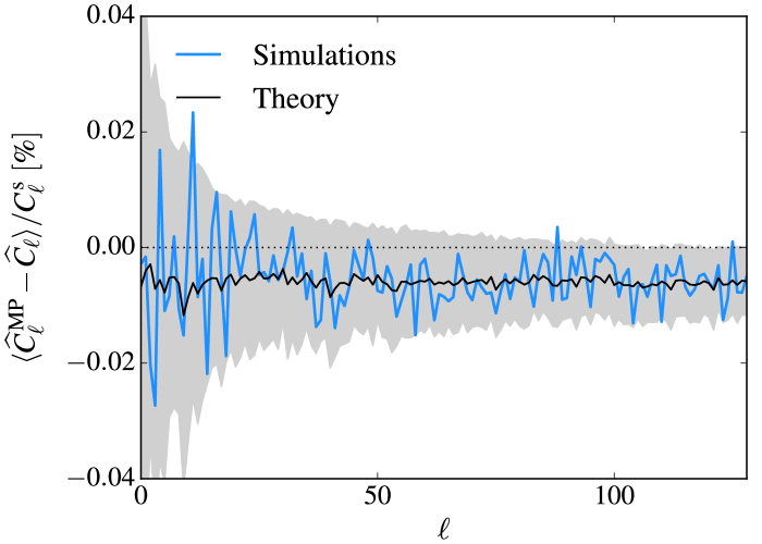
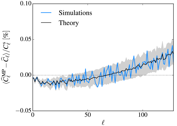
Figure 1: The bias introduced by mode projection shows a non-trivial dependence on the shape of signal and template power spectra. Left-hand panel: Result for a flat signal power spectrum, $C_{\ell{}}^{\,\mathrm{s}}=\mathrm{const.}$ Right-hand panel: Bias comparison for a red signal power spectrum, $C_{\ell{}}^{\,\mathrm{s}}\propto(\ell+1)^{-2}$. The gray regions indicate the empirical $2\text{-}\sigma$ standard error of the mean as derived from the simulations.

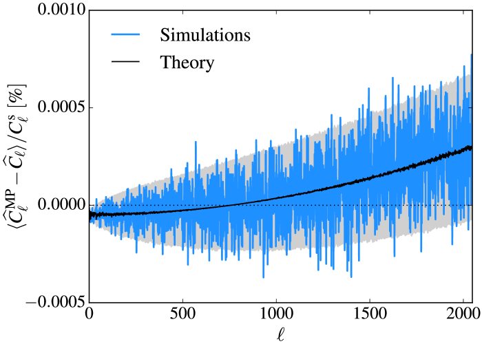
Figure 2: The scheme is efficient enough to be applicable to high-resolution data sets. Same as Fig. 1, but plotting results for an increased maximum multipole moment of $\ell_{\mathrm{max}}=2048$, derived on an off-the-shelf desktop computer.

3.2 Number of templates

Still considering a full sky analysis, we now test the scaling behaviour of the PCL power spectrum bias induced by mode projection with the number of templates used in the cleaning procedure. To this end we repeated the analysis of 1000 simulated realizations of the data set, drawn from $C_{\ell{}}^{\,\mathrm{s}}\propto(\ell+1)^{-2}$, which we have now cleaned with 100 randomly generated template maps. The result is shown in Fig. 3; compared to the single template case, we observe a bias that is larger by two orders of magnitude. In case they are not or only mildly correlated, we indeed expect to see an approximately linear scaling with the number of templates, since the independent estimation of the cleaning amplitudes allows the removal of power in one Fourier mode per template. This observation is of particular relevance to current and next generation surveys since a robust analysis may require the projection of the order of hundreds or thousands of templates. A reliable means to correct for a potentially large resulting bias is therefore paramount.

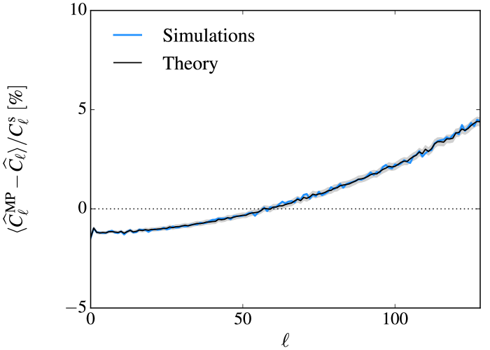
Figure 3: The bias increases approximately linearly with the number of templates projected. Same as Fig. 1, but now projecting 100 instead of a single template. The observed bias becomes larger by about two orders of magnitude.

3.3 Sky fraction

In a further set of tests, we probe the impact of a limited sky fraction used for the analysis on the bias of the power spectra computed with template projection. In the left-hand panel of Fig. 4, we show the bias for a cut-sky analysis restricted to $f_{\mathrm{sky}}=1\%$. For large to intermediate sky fractions, we observe a scaling approximately proportional to $1/f_{\mathrm{sky}}$. We note that for small sky fractions however, this simplified relationship is expected to break down. In the right-hand panel of Fig. 4, we remove the contribution of 100 templates while simultaneously restricting the analysis to $f_{\mathrm{sky}}=1\%$. In that case, the relative bias can become larger than unity. The agreement between simulations and analytical calculation remains good.

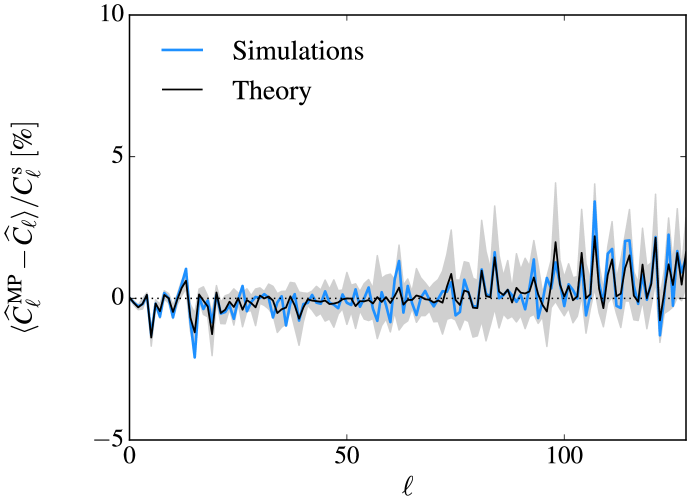
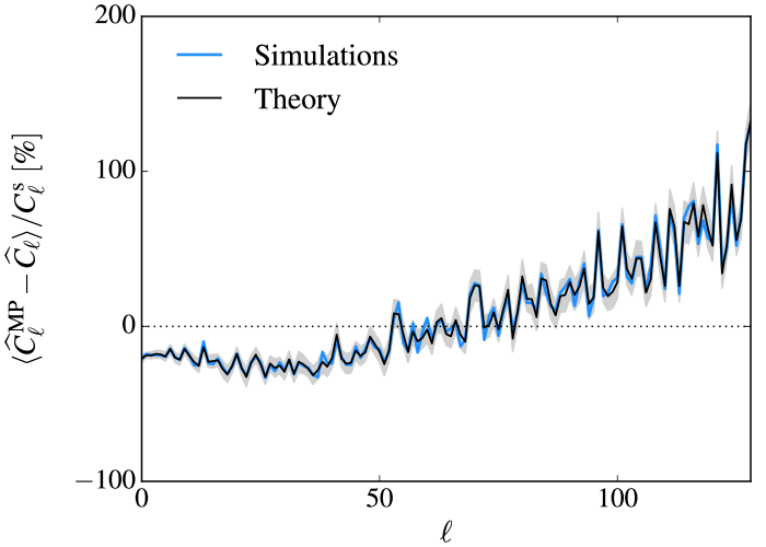
Figure 4: Left-hand panel: The bias is approximately inversely proportional to the sky fraction available to the analysis. Same as Fig. 1, but now restricting the analysis to $f_{\mathrm{sky}}=1\%$. The larger sample variance leads to an increased scatter. Right-hand panel: Projecting a large number of templates on a comparatively small sky area can lead to bias values in excess of unity. Same as Fig. 1, but marginalizing over 100 templates on $f_{\mathrm{sky}}=1\%$ of the sky.

3.4 Estimator variance

Implementing mode projection into PCL alters the covariance properties of power spectrum estimates. While a full analysis is beyond the scope of this paper, we provide a qualitative assessment of changes in the estimator variance. In general, the statistical properties of estimates can be characterized using an analytical description, simulations, or resampling methods like bootstrapping. Here, we analyzed the empirical variance of $100\,000$ full-sky power spectra, computed from signal simulations drawn from $C_{\ell{}}^{\,\mathrm{s}}\propto(\ell+1)^{-2}$. We directly compared the debiased results obtained from maps that have been cleaned by a single template on the one hand, and the power spectra computed without mode projection on the other hand. In general, we find an increased variance with a multipole dependence resembling the general shape of the bias discussed in the last paragraphs. Interestingly, as visualized in Fig. 5, changes in the variance depend on the details of the debiasing procedure. As mentioned in Sect. 2, the analytical expression used to debias the results may depend in a non-trivial way on the signal power spectrum, leaving us with two options to proceed. It is possible to either use the current (biased) signal estimate $\widehat{C}_{\ell{}}^{\,\mathrm{s}}$ for an iterative correction, or to assume a prior power spectrum $C_{\ell{}}^{\,\mathrm{s}}$ in the calculation. While both approaches lead to unbiased signal power spectrum estimates in the ensemble average, the estimator variance will be different. The additional information introduced by a prior results in a deterministic bias correction, independent of the signal realization, that in turn leads to a decreased estimator variance in multipole regions that are most effectively cleaned.

For flat signal and template power spectra, we can provide an order-of-magnitude estimate of the expected increase in variance of iteratively-debiased signal power spectra. Considering the number of modes removed by projecting $n$ templates, we obtain a rough estimate of the variance ratio of power spectra computed with and without mode projection,

$$\left.\mathrm{Var}\left(\widehat{C}_{\ell{}}^{\,\mathrm{s,\mathrm{MP}}}\right)\middle/\mathrm{Var}\left(\widehat{C}_{\ell{}}^{\,\mathrm{s}}\right)\right.\sim\frac{2(\ell_{\mathrm{max}}+1)^{2}}{f_{\mathrm{sky}}\left[(\ell_{\mathrm{max}}+1)^{2}-n\right]}\,,$$ (33)

where $f_{\mathrm{sky}}$ is the sky fraction used in the analysis.

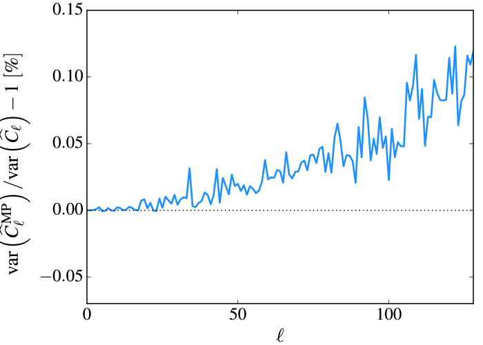
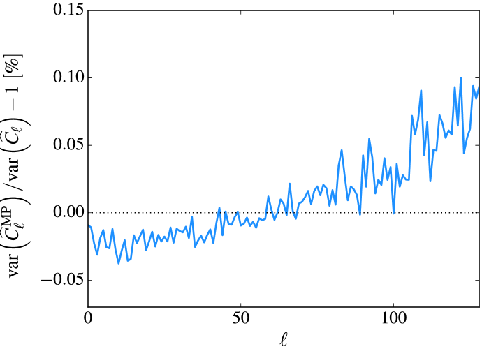
Figure 5: Mode projection induces changes in the estimator variance that depend on the details of the bias removal. Debiasing power spectrum estimates iteratively increases the estimator variance on all scales (left-hand panel), while the use of a prior power spectrum can result in a multipole range with reduced variance (right-hand panel).

4 Summary and conclusions

In modern cosmology, two-point correlation function measurements play a fundamental role in constraining theoretical models with observational data. In practical application, however, extracting statistical information about cosmological signals is often hampered by the presence of contaminants. As a consequence, a number of strategies have been developed to mitigate their impact on the scientific analysis. Here, we focus on mode projection, an algorithm that allows one to marginalize over templates constructed to describe the spatial patterns of possible systematic effects (Rybicki & Press, 1992). While it can be straightforwardly implemented into optimal methods, the application to the popular pseudo-$C_{\ell}$ (PCL) estimator, so far, has remained elusive.

In this paper, we have developed a framework to integrate mode projection into PCL estimation algorithms. We have shown that a naive projection of templates in general leads to biased power spectrum estimates. Based on a rigorous mathematical treatment, we then derived exact closed-form equations for the estimator bias. Recasting the analytical expressions allowed us to compute them efficiently, thereby preserving the overall ${{\cal O}\!\left(\ell_{\mathrm{max}}^{3}\right)}$ time complexity of PCL algorithms.

Applied to a large number of simulations with various input parameters, we have systematically studied the impact of mode projection on PCL power spectrum estimates. We identified a nontrivial dependence of the cleaning procedure on the shape of signal and template power spectra. We further studied the scaling of the bias with the band limit of the maps, number of templates projected, and sky fraction available to the analysis, and discussed the impact of mode projection on the covariance properties of the power spectrum estimates. In all cases, we found a good agreement between the bias observed in simulations and our analytical prediction. We conclude that the framework presented here allows for a reliable correction of power spectrum estimates to obtain unbiased results. Possible future extensions of the algorithm include the generalization to spin-2 fields to allow more robust measurements of, for example, the cosmic shear signal (e.g., Bacon et al., 2000; Kaiser et al., 2000; Wittman et al., 2000; Lin et al., 2012; Kilbinger et al., 2013; Kuijken et al., 2015; Becker et al., 2016), or the CMB polarization power spectrum (e.g., Kovac et al., 2002; BICEP2 Collaboration et al., 2014; Naess et al., 2014; The Polarbear Collaboration: P. A. R. Ade et al., 2014; Planck Collaboration et al., 2016).

Effective strategies for systematics mitigation are instrumental to fully exploring the information content of ongoing and future large scale structure surveys like the Sloan Digital Sky Survey (York et al., 2000), the Dark Energy Survey (Frieman & Dark Energy Survey Collaboration, 2013), or observations planned with the Dark Energy Spectroscopic Instrument (Levi et al., 2013), or the Large Synoptic Survey Telescope (LSST Science Collaboration et al., 2009). The results of our studies indicate that the combination of mode projection and pseudo-$C_{\ell}$ power spectrum estimation offers an attractive means to robustly measure the two-point correlation function in the presence of contaminants, an important milestone on the way to reliable clustering estimates.

Appendix A Equivalence between mode projection and masking

Analyzing a specifically designed toy experiment, we now demonstrate the conceptual equivalence of mode projection and masking. For a data map with $n_{\mathrm{pix}}$ pixels, where $n_{\mathrm{pix}}$ is large, we consider a template with real space representation $(f)_{i}=\delta_{ij}$, i.e., only a single template pixel with index $j$ is different from zero. We will now show that the mode projection algorithm yields identical results compared to a PCL analysis, where pixel $j$ has been masked.

Applying the cleaning procedure Eq. (7) to obtain the filtered data vector, we find

$$(\widetilde{d})_{i}=\begin{cases}0&i=j\\ d_{i}&\mathrm{otherwise.}\end{cases}$$ (34)

To debias mode projection results requires the exact knowledge of the template power spectrum, a quantity that will depend on the details of the pixelization scheme in our test case (e.g., pixel shape, size, position, assumed sub-pixel model). In favour of a fully analytical treatment of the problem, however, we choose to work with an approximate expression of the template power spectrum instead,

$$\widehat{C}_{\ell{}}^{\,\mathrm{f}}\approx\frac{4\pi}{n_{\mathrm{pix}}^{2}}\,.$$ (35)

Since maximally localized fields in real space in general do not possess a well-defined band limit in Fourier space, we further impose a hard limit at $\ell_{\mathrm{max}}$, chosen such that the total number of Fourier modes equals the number of pixels, $(\ell_{\mathrm{max}}+1)^{2}=n_{\mathrm{pix}}$, finding

$$\sum_{\ell}(2{\ell{}}+1)\widehat{C}_{\ell{}}^{\,\mathrm{f}}=\frac{4\pi}{n_{\mathrm{pix}}}\,.$$ (36)

The matrix used to debias power spectrum measurements with mode projection (Eqs. (15) and (16)) then takes the simple form

$$(\mathbb{1}+B)_{\ell_{1}\ell_{2}}=\left(1-\frac{2}{n_{\mathrm{pix}}}\right)\cdot\delta_{\ell_{1}\ell_{2}}+\frac{2\ell_{2}+1}{n_{\mathrm{pix}}^{2}}\,.$$ (37)

After a full analysis of the template projection algorithm for this specific case, we now derive the corresponding equations for a PCL power spectrum estimator. Masking the input map will set the pixel with index $j$ to zero while leaving all other entries untouched. Using identical assumptions as before, the power spectrum of the mask $W=1-f$ is approximately given by

$$\widehat{C}_{\ell{}}^{\,\mathrm{w}}\approx\begin{cases}4\pi\left(1-\frac{1}{n_{\mathrm{pix}}}\right)^{2}&\ell=0\\ \frac{4\pi}{n_{\mathrm{pix}}^{2}}&\mathrm{otherwise.}\end{cases}$$ (38)

Using this expression, we obtain for the PCL coupling matrix, see Eq. (42) below,

$$M_{\ell_{1}\ell_{2}} =\frac{2\ell_{2}+1}{4\pi}\left[4\pi\left(1-\frac{2}{n_{\mathrm{pix}}}\right)\begin{pmatrix}\ell_{1}&\ell_{2}&0\\ 0&0&0\end{pmatrix}^{2}\right.$$

$$+\left.\frac{4\pi}{n_{\mathrm{pix}}^{2}}\sum_{\ell_{3}}(2{\ell{{}_{3}}}+1)\begin{pmatrix}\ell_{1}&\ell_{2}&\ell_{3}\\ 0&0&0\end{pmatrix}^{2}\right]$$

$$=\left(1-\frac{2}{n_{\mathrm{pix}}}\right)\cdot\delta_{\ell_{1}\ell_{2}}+\frac{2\ell_{2}+1}{n_{\mathrm{pix}}^{2}}\,.$$ (39)

Finding identical results for the filtered (mode projection) or masked (PCL power spectrum estimation) data vector as well as for the debiasing procedures (Eqs. (37) and (A)), we conclude the full equivalence of the two schemes.

We note in closing that the effect of any binary mask can therefore be interpreted as projecting a collection of template maps. In this case, each template would be non-zero only for a single pixel that falls inside the masked area. For more general weight maps that are not restricted to the numerical values zero and one, this equivalence is no longer true and we have to resort to the more complicated schemes discussed in Sects. 2.3 and 2.4.

Appendix B PCL coupling kernels

We start from the Gaunt integral that allows to express the product of three spin-0 spherical harmonics in terms of Wigner 3j symbols (Gaunt, 1929),

$$\int\mathrm{d}\bm{n}\,Y_{\ell_{1}m_{1}}(\bm{n}) \,Y_{\ell_{2}m_{2}}(\bm{n})\,Y_{\ell_{3}m_{3}}(\bm{n})$$

$$=\left[\frac{(2{\ell{{}_{1}}}+1)(2{\ell{{}_{2}}}+1)(2{\ell{{}_{3}}}+1)}{4\pi}\right]^{1/2}$$

$$\times\begin{pmatrix}\ell_{1}&\ell_{2}&\ell_{3}\\ 0&0&0\end{pmatrix}\begin{pmatrix}\ell_{1}&\ell_{2}&\ell_{3}\\ m_{1}&m_{2}&m_{3}\end{pmatrix}\,.$$ (40)

Given this useful relation, the following Fourier space representation of the coupling kernel can straightforwardly be obtained from Eq. (2.3) (Hivon et al., 2002),

$$K_{\ell_{1}m_{1}\ell_{2}m_{2}}\\ =\sum_{\ell_{3}m_{3}}w_{\ell{{}_{3}}m{{}_{3}}}(-1)^{m_{2}}\left[\frac{(2\ell_{1}+1)(2\ell_{2}+1)(2\ell_{3}+1)}{4\pi}\right]^{1/2}\\ \times\begin{pmatrix}\ell_{1}&\ell_{2}&\ell_{3}\\ 0&0&0\end{pmatrix}\begin{pmatrix}\ell_{1}&\ell_{2}&\ell_{3}\\ m_{1}&-m_{2}&m_{3}\end{pmatrix}\,,$$ (41)

where we have introduced the spherical harmonic coefficients of the mask, $w_{\ell{}m{}}$.

Making use of the orthogonality relations of the Wigner 3j symbols (e.g., Edmonds, 1996), the coupling matrix that connects the ensemble average of full- and cut-sky power spectra is given by

$$M_{\ell_{1}\ell_{2}}=\frac{2\ell_{2}+1}{4\pi}\sum_{\ell_{3}}(2{\ell{{}_{3}}}+1)\widehat{C}_{\ell{{}_{3}}}^{\,\mathrm{w}}\begin{pmatrix}\ell_{1}&\ell_{2}&\ell_{3}\\ 0&0&0\end{pmatrix}^{2}\,.$$ (42)

It is a function of the mask power spectrum $\widehat{C}_{\ell{}}^{\,\mathrm{w}}$ only.

References

- Awan et al. (2016) Awan H., et al., 2016, ApJ, 829, 50
- BICEP2 Collaboration et al. (2014) BICEP2 Collaboration et al., 2014, Physical Review Letters, 112, 241101
- BICEP2/Keck and Planck Collaborations et al. (2015) BICEP2/Keck and Planck Collaborations et al., 2015, Physical Review Letters, 114, 101301
- Bacon et al. (2000) Bacon D. J., Refregier A. R., Ellis R. S., 2000, MNRAS, 318, 625
- Becker et al. (2016) Becker M. R., et al., 2016, Phys. Rev. D, 94, 022002
- Bennett et al. (1992) Bennett C. L., et al., 1992, ApJ, 396, L7
- Bennett et al. (2003) Bennett C. L., et al., 2003, ApJS, 148, 97
- Beutler et al. (2011) Beutler F., et al., 2011, MNRAS, 416, 3017
- Blake & Wall (2002) Blake C., Wall J., 2002, MNRAS, 329, L37
- Bond et al. (1998) Bond J. R., Jaffe A. H., Knox L., 1998, Phys. Rev. D, 57, 2117
- Borrill (1999) Borrill J., 1999, Phys. Rev. D, 59, 027302
- Coil et al. (2008) Coil A. L., et al., 2008, ApJ, 672, 153
- Crocce et al. (2016) Crocce M., et al., 2016, MNRAS, 455, 4301
- Croom et al. (2005) Croom S. M., et al., 2005, MNRAS, 356, 415
- Edmonds (1996) Edmonds A. R., 1996, Angular Momentum in Quantum Mechanics. Investigations in Physics Series, Princeton University Press, http://press.princeton.edu/titles/478.html
- Eisenstein et al. (2005) Eisenstein D. J., et al., 2005, ApJ, 633, 560
- Elsner & Wandelt (2013) Elsner F., Wandelt B. D., 2013, A&A, 549, A111
- Elsner et al. (2016) Elsner F., Leistedt B., Peiris H. V., 2016, MNRAS, 456, 2095
- Eriksen et al. (2004) Eriksen H. K., Banday A. J., Górski K. M., Lilje P. B., 2004, ApJ, 612, 633
- Feldman et al. (1994) Feldman H. A., Kaiser N., Peacock J. A., 1994, ApJ, 426, 23
- Fowler et al. (2010) Fowler J. W., et al., 2010, ApJ, 722, 1148
- Frieman & Dark Energy Survey Collaboration (2013) Frieman J., Dark Energy Survey Collaboration 2013, in American Astronomical Society Meeting Abstracts #221. p. 335.01, http://adsabs.harvard.edu/abs/2013AAS...22133501F
- Gaunt (1929) Gaunt J. A., 1929, Royal Society of London Philosophical Transactions Series A, 228, 151
- Górski et al. (2005) Górski K. M., Hivon E., Banday A. J., Wandelt B. D., Hansen F. K., Reinecke M., Bartelmann M., 2005, ApJ, 622, 759
- Gundersen et al. (1995) Gundersen J. O., et al., 1995, ApJ, 443, L57
- Halverson et al. (2002) Halverson N. W., et al., 2002, ApJ, 568, 38
- Hanany et al. (2000) Hanany S., et al., 2000, ApJ, 545, L5
- Hancock et al. (1994) Hancock S., Davies R. D., Lasenby A. N., de La Cruz C. M. G., Watson R. A., Rebolo R., Beckman J. E., 1994, Nature, 367, 333
- Hermit et al. (1996) Hermit S., Santiago B. X., Lahav O., Strauss M. A., Davis M., Dressler A., Huchra J. P., 1996, MNRAS, 283, 709
- Hinshaw et al. (2003) Hinshaw G., et al., 2003, ApJS, 148, 135
- Hinshaw et al. (2007) Hinshaw G., et al., 2007, ApJS, 170, 288
- Hivon et al. (2002) Hivon E., Górski K. M., Netterfield C. B., Crill B. P., Prunet S., Hansen F., 2002, ApJ, 567, 2
- Ho et al. (2012) Ho S., et al., 2012, ApJ, 761, 14
- Huffenberger & Wandelt (2010) Huffenberger K. M., Wandelt B. D., 2010, ApJS, 189, 255
- Huterer et al. (2013) Huterer D., Cunha C. E., Fang W., 2013, MNRAS, 432, 2945
- Kaiser et al. (2000) Kaiser N., Wilson G., Luppino G. A., 2000, ArXiv e-prints, astro-ph/0003338
- Kalus et al. (2016) Kalus B., Percival W. J., Bacon D. J., Samushia L., 2016, MNRAS, 463, 467
- Kilbinger et al. (2013) Kilbinger M., et al., 2013, MNRAS, 430, 2200
- Kim et al. (2014) Kim J.-W., et al., 2014, MNRAS, 438, 825
- Kovac et al. (2002) Kovac J. M., Leitch E. M., Pryke C., Carlstrom J. E., Halverson N. W., Holzapfel W. L., 2002, Nature, 420, 772
- Kuijken et al. (2015) Kuijken K., et al., 2015, MNRAS, 454, 3500
- LSST Science Collaboration et al. (2009) LSST Science Collaboration et al., 2009, ArXiv e-prints, 0912.0201
- Leistedt & Peiris (2014) Leistedt B., Peiris H. V., 2014, MNRAS, 444, 2
- Leistedt et al. (2013) Leistedt B., Peiris H. V., Mortlock D. J., Benoit-Lévy A., Pontzen A., 2013, MNRAS, 435, 1857
- Leistedt et al. (2016) Leistedt B., et al., 2016, ApJS, 226, 24
- Levi et al. (2013) Levi M., et al., 2013, preprint (arXiv:1308.0847)
- Lin et al. (2012) Lin H., et al., 2012, ApJ, 761, 15
- Lueker et al. (2010) Lueker M., et al., 2010, ApJ, 719, 1045
- Maller et al. (2005) Maller A. H., McIntosh D. H., Katz N., Weinberg M. D., 2005, ApJ, 619, 147
- Naess et al. (2014) Naess S., et al., 2014, J. Cosmology Astropart. Phys., 10, 007
- Netterfield et al. (1997) Netterfield C. B., Devlin M. J., Jarosik N., Page L., Wollack E. J., 1997, ApJ, 474, 47
- Norberg et al. (2001) Norberg P., et al., 2001, MNRAS, 328, 64
- Planck Collaboration et al. (2014) Planck Collaboration et al., 2014, A&A, 571, A15
- Planck Collaboration et al. (2016) Planck Collaboration et al., 2016, A&A, 594, A11
- Reid et al. (2010) Reid B. A., et al., 2010, MNRAS, 404, 60
- Reinecke (2011) Reinecke M., 2011, A&A, 526, A108+
- Reinecke & Seljebotn (2013) Reinecke M., Seljebotn D. S., 2013, A&A, 554, A112
- Ross et al. (2011) Ross A. J., et al., 2011, MNRAS, 417, 1350
- Ross et al. (2012) Ross A. J., et al., 2012, MNRAS, 424, 564
- Ross et al. (2016) Ross A. J., et al., 2016, preprint (arXiv:1607.03145)
- Rybicki & Press (1992) Rybicki G. B., Press W. H., 1992, ApJ, 398, 169
- Saha et al. (2008) Saha R., Prunet S., Jain P., Souradeep T., 2008, Phys. Rev. D, 78, 023003
- Schaeffer (2013) Schaeffer N., 2013, Geochemistry, Geophysics, Geosystems, 14, 751
- Scranton et al. (2002) Scranton R., et al., 2002, ApJ, 579, 48
- Slosar et al. (2004) Slosar A., Seljak U., Makarov A., 2004, Phys. Rev. D, 69, 123003
- Smith et al. (2009) Smith K. M., Senatore L., Zaldarriaga M., 2009, J. Cosmology Astropart. Phys., 9, 6
- Smoot et al. (1992) Smoot G. F., et al., 1992, ApJ, 396, L1
- Tegmark (1997) Tegmark M., 1997, Phys. Rev. D, 55, 5895
- Tegmark et al. (1998) Tegmark M., Hamilton A. J. S., Strauss M. A., Vogeley M. S., Szalay A. S., 1998, ApJ, 499, 555
- Tegmark et al. (2004) Tegmark M., et al., 2004, ApJ, 606, 702
- The Polarbear Collaboration: P. A. R. Ade et al. (2014) The Polarbear Collaboration: P. A. R. Ade et al., 2014, ApJ, 794, 171
- Totsuji & Kihara (1969) Totsuji H., Kihara T., 1969, PASJ, 21, 221
- Wittman et al. (2000) Wittman D. M., Tyson J. A., Kirkman D., Dell’Antonio I., Bernstein G., 2000, Nature, 405, 143
- York et al. (2000) York D. G., et al., 2000, AJ, 120, 1579
- Zehavi et al. (2002) Zehavi I., et al., 2002, ApJ, 571, 172