Semiclassical Hartree-Fock theory of a rotating Bose-Einstein condensation

Abstract

In this paper, we investigate the thermodynamic behavior of a rotating Bose-Einstein condensation with non-zero interatomic interactions theoretically. The analysis relies on a semiclassical Hartree-Fock approximation where an integral is performed over the phase space and function of the grand canonical ensemble is derived. Subsequently, we use this result to derive several thermodynamic quantities including the condensate fraction, critical temperature, entropy and heat capacity. Thereby, we investigate the effect of the rotation rate and interactions parameter on the thermodynamic behavior. The role of finite size is discussed. Our approach can be extended to consider the rotating condensate in optical potential.

I Introduction

One of the most remarkable characteristics of a Bose-Einstein condensate (BEC) is its response to rotate with superfluid nature madison ; mattews ; codd . This property makes the inclusion of interatomic interactions an essential requirement for the correct description of the system. In spite of the basic phenomenon of BEC may be illustrated with an ideal gas, it became clear that the interatomic interactions play a predominant role in determining both the qualitative and the quantitative properties of the ultracold gases, especially, for temperatures below the transition.

However, the statistical mechanics of the interacting system remains unsolvable and one has to resort to approximated schemes such as Hartree-Fock (HF) approximations dal . In this respect, the semiclassical HF description has produced excellent agreement with experimentally measured equilibrium quantities gio . While HF is still very useful, since it does take into account interatomic interactions and being a mean-field theory, it should give rise to a correct qualitative picture of the phase transition. Many open questions remain predominantly related to exploring the effects of interatomic interactions on the behavior of this system under different circumstances tammuz . These include: the effect of interaction on the BEC transition temperature strn ; sss ; the heat capacity for the system, which enabled us to discuss the order of phase transition ket1 ; Shiozaki and the entropy of the system Olf , which required to investigate the adiabatic cooling of the boson system in lattice to magnetic ordering.

In the present paper, motivated by the careful study of harmonically confined Bose gas in a rotating trap Kling ; fetter ; qiang , we employed a developed semiclassical approximation. The sum over the discrete spectrum for the grand thermodynamic potential is converted into an integral over phase space. Performing the integral over this phase space required to calculate many system parameters, such as the condensate density, the effective potential as well as the chemical potential. However, all of them may be self-consistently parametrized using the Hartree-Fock approximation Sinha ; Sandoval ; Jae . Using the thermodynamical potential, the condensed fraction, the transition temperature, entropy and the heat capacity are calculated. Our numerical results are calculated by using the trap parameters of Coddington et al. experimentcodd . The calculated results showed that the thermodynamic properties depend strongly on the interatomic interaction and the rotation rate on the whole temperature range.

The paper is planned as follows: section two includes the system definition and a systematic method for calculating the accurate thermodynamic potential. The thermodynamic quantities are given in section three. Conclusion is given in the last section.

II Basic formalism

We consider a mesoscopic sample of weakly interacting $N$ bosonic atoms of mass $m$ placed in an axially symmetric harmonic potential, $V_{trap}(r_{\bot},z)=\frac{m}{2}(\omega_{\bot}^{2}r_{\bot}^{2}+\omega_{z}^{2}z^{2})$, with $r_{\bot}^{2}=x^{2}+y^{2}$ is the perpendicular radius and $\{\omega_{\bot}\equiv\omega_{x}=\omega_{y},\omega_{z}\}$ are the effective trapping frequencies of the harmonic potential. The gas is set in rotation using an anisotropic quadratic potential $V$ in the $xy$ plane, rotating at angular frequency $\Omega$ around the $z$ axis. In the rotating frame, this stirring potential reads bargi ; peta ,

$$V_{rot}(r_{\bot},z)=\frac{1}{2}m[\omega_{\bot}^{2}(\kappa_{+}\kappa_{-})r_{\bot}^{2}+\omega_{z}^{2}z^{2}]$$ (1)

where $\kappa_{\pm}={(1\mp\alpha)}$ and $\alpha=\frac{\Omega}{\omega_{\bot}}$, is the rotation rate.

The Hamiltonian describing the interacting atomic gas in the potential (1) is given bycooper

$$H=\frac{|{\bf{p_{\bot}}}-m{\bf\Omega\times r_{\bot}}|^{2}}{2m}+\frac{p_{z}^{2}}{2m}+V_{eff}(r_{\bot},z),$$ (2)

where $V_{eff}(r_{\bot},z)$ is the effective potential for rotating interacting condensate boson,

$$V_{eff}(r_{\bot},z)=V_{rot}(r_{\bot},z)+2g[n_{th}(r_{\bot},z)+n_{0}(r_{\bot},z)],$$ (3)

with $g=\frac{4\pi\hbar^{2}a}{m}$ is the interaction strength, $n_{0}(r_{\bot},z)$ and $n_{th}(r_{\bot},z)$ are the density of condensate and thermal atoms in the rotating frame.

Usually, BEC is described within the grand canonical ensemble. All relevant thermodynamic quantities can be calculated from partial derivative of the grand potential $q$, which is the logarithm of the grand canonical partition function kir ; pat .

$$q(\alpha,T)=-\sum_{n=0}^{\infty}\ln(1-e^{-\beta(E_{n}-\mu(\alpha))})$$ (4)

where $\beta=1/(k_{B}T)$ and $\mu(\alpha)$ is the chemical potential of the rotating Bose condensate boson. It is convenient to separate out the ground state contribution and expand the logarithm, $\ln(1-y)=-\sum_{j=1}^{\infty}\frac{y^{j}}{j}$, to express $q$ as a sum over Bose-Einstein distributionket1 , $N_{n}=\frac{{\textsc{z}}e^{-\beta E_{n}}}{1-{\textsc{z}}e^{-\beta E_{n}}}=\sum_{j=1}^{\infty}{\textsc{z}}^{j}\sum_{n=0}^{\infty}e^{-j\beta E_{n}}$. Thus, Eq.(4) can be rewritten as,

$$q(\alpha,T) = q_{o}+\sum_{j}\frac{{\textsc{z}}^{j}}{j}\sum_{n=1}^{\infty}e^{-j\beta E_{n}}$$ (5)

$$\equiv q_{0}+q_{th}$$

where $q_{o}=-\ln(1-{\textsc{z}})$ is the grand potential for the atoms in the ground state, with ${\textsc{z}}=e^{\beta\mu(\alpha)}$ is the effective fugacity and $q_{th}$ is the grand potential for thermal atoms.

The sum in Eq.(5) cannot be evaluated analytically in a closed form. Another possible way to do this analysis is to approximate the sum by integral (semiclassical approximation) over the phase space or converting the sum into an integral weighted by an appropriate smooth density of states (DOS), $\rho(E)$. These two approximations required that the condition $K_{B}T$ is much larger than the energy level spacing of the system.

III Semiclassical approximation

III.1 Hartree-Fock approximation

The sum over $n$ in Eq.(5) can be converted into an integral over the phase space by replacing the discrete $E_{n}$ with a continuous variable $\epsilon({\bf r;p})$ depends on position $\bf r$ and momentum $\bf p$, which corresponds to the classical energy associated with the single-particle Hamiltonian for the system given in Eq.(2). This does not take into account the contribution from $n=0$. In three dimensions, there is on average one quantum state per volume of phase space $(2\pi\hbar)^{3}$. Integrating over all phase space and dividing by this factor thus yields the thermodynamic potential, $q_{th}$, for the atoms that occupied the excited states, Sinha ; hau ,

$$q_{th}({\bf p,r}) = -\frac{1}{(2\pi\hbar)^{3}}\sum_{j=1}^{\infty}\frac{{\textsc{z}}^{j}}{j}\int{d^{2}p_{\bot}dp_{z}d^{2}r_{\bot}dz}$$ (6)

$$\times e^{-j\beta[\frac{|{\bf{p_{\bot}}}-m{\bf\Omega\times r_{\bot}}|^{2}}{2m}+\frac{p_{z}^{2}}{2m}+V_{eff}(r_{\bot},z)]}$$

After doing the $p$ integration by making the change of variables ${\bf p\to p}-m{\bf\Omega}\times{\bf r}$, the integral in Eq.(6) takes the same form as in the absence of synthetic magnetic field with an effective frequencies $\sqrt{\omega_{\bot}^{2}(\kappa_{+}\kappa_{-})}$ and $\omega_{z}$, respectively. Finally, the local grand potential is given by

$$q_{th}({\bf r})=\frac{1}{\lambda_{th}^{3}}\int\sum_{j=1}^{\infty}\frac{{\textsc{z}}^{j}}{j^{5/2}}\int e^{-j\beta V_{eff}(r_{\bot},z)}{d^{2}r_{\bot}dz}$$ (7)

where $\lambda_{th}=\sqrt{\frac{2\pi\hbar^{2}}{mk_{B}T}}$ is the thermal de-Broglie wavelength. However, calculating the phase space integral required calculating some of the system parameters, include the effective potential, chemical potential and the densities of condensate and thermal atoms. The above mentioned parameters can be calculated using the Hartree-Fock approximation.

In the self-consistent Hartree-Fock model, the thermal atoms are treated as a non-interacting gas with density $n_{th}(r_{\bot},z)$ confined by the effective potential $V_{eff}(r_{\bot},z)$ given in Eq.(3). The densities of the thermal and condensate component are given as a solution of the two coupled equations: the thermal atoms satisfy Schrödinger’s equation

$$\Big{[}\frac{|{\bf{p_{\bot}}}-m{\bf\Omega\times r_{\bot}}|^{2}}{2m}+\frac{p_{z}^{2}}{2m} + V_{eff}(r_{\bot},z)\Big{]}\psi_{i}(r_{\bot},z)$$ (8)

$$= \epsilon_{i}\psi_{i}(r_{\bot},z)$$

and the condensate part satisfies the time independent Gross-Pitaevskii equation,

$$\Big{[}\frac{|{\bf{p_{\bot}}}-m{\bf\Omega\times r_{\bot}}|^{2}}{2m}+\frac{p_{z}^{2}}{2m} + V_{rot}(r_{\bot},z)+gn_{0}(r_{\bot},z)$$

$$+2gn_{th}(r_{\bot},z)\Big{]}\phi(r_{\bot},z) = \mu(\alpha)\phi(r_{\bot},z),$$ (9)

Eq’s. (6), (8) and (9) along with the constraint that the total number of atoms $N$ is fixed,

$$N=\int n_{th}{(r_{\bot},z)}d^{2}r_{\bot}dz+\int n_{0}{(r_{\bot},z)}d^{2}r_{\bot}dz$$ (10)

form a closed set of equations which must be solved self-consistently.

Both the condensate density $n_{0}{(r_{\bot},z)}$ and $\mu(\alpha)$ can be calculated from the time independent Gross-Pitaevskii equation for the condensate part, Eq.(9). Moreover, the situation may be simplified by taking advantage of the small density of the thermal component (at very low temperature, this requirement may be achieved). In this case, the effect of thermal atoms on the condensate can be neglected and $n_{0}(r_{\bot},z)$ is given by the Thomas-Fermi approximation (the kinetic energy term is omitted) of Eq.(9), leaving an algebraic equation for the condensate density,

$$n_{0}(r_{\bot},z)=\frac{\mu(\alpha)-V_{rot}(r_{\bot},z)}{g}$$ (11)

For all $\mu(\alpha)>V_{rot}(r_{\bot},z)$ and $n_{0}(r_{\bot},z)$ = 0 elsewhere. Substituting from Eq.(1) into Eq.(11) leads to,

$$n_{0}(r_{\bot},z)=\frac{\mu(\alpha)}{g}\Big{[}1-\frac{r_{\bot}^{2}}{R_{\bot}^{2}(\alpha)}-\frac{z^{2}}{R_{z}^{2}(\alpha)}\Big{]}$$ (12)

where

$$R_{\bot}(\alpha)=\sqrt{\frac{2\mu(\alpha)}{m\omega_{\bot}^{2}(\kappa_{+}\kappa_{-})}}\ {\rm and}\ R_{z}(\alpha)=\sqrt{\frac{2\mu(\alpha)}{m\omega_{z}^{2}}},$$ (13)

is the Thomas-Fermi radius at which the condensate density drops to zero along the $r_{\bot}$ or $z$ axis. Both $R_{\bot}(\alpha)$ and $R_{z}(\alpha)$ accounted for the condensate radius in terms of the trap parameters. These two radius can be expressed in terms of the condensate number of atoms through the relation between $\mu(\alpha)$ and $N_{0}$. The relation between $\mu(\alpha)$ and $N_{0}$ may be founded by integrating (12) over the ellipsoid with semi-axes $R_{\bot}$ and $R_{z}$,

$$N_{0} = \int n_{0}(r_{\bot},z)d^{2}r_{\bot}dz$$ (14)

$$= \frac{8\pi}{15}\frac{\mu(\alpha)}{g}(R_{\bot}^{2}(\alpha)R_{z}(\alpha))=\frac{8\pi}{15}\frac{\mu(\alpha)}{g}{\bar{R}}^{3}(\alpha)$$

$\bar{R}(\alpha)$ is representing the geometric mean $(R_{\bot}^{2}(\alpha)R_{z}(\alpha))^{1/3}$. Eq.(14) can be inverted to give ${\mu(\alpha)}$ in terms of $N_{0}$ such as

$$\mu(\alpha)=\frac{1}{2}\hbar\omega_{g}\Big{(}\frac{15N_{0}a}{a_{har}}\big{)}^{2/5}(\kappa_{+}\kappa_{-})^{\frac{2}{5}}=\mu(0)(\kappa_{+}\kappa_{-})^{\frac{2}{5}}$$ (15)

where $\mu(0)=\frac{1}{2}\hbar\omega_{g}\Big{(}\frac{15N_{0}a}{a_{har}}\big{)}^{2/5}$ is the chemical potential for non rotating condensate, $a$ is the s-wave scattering length, $a_{har}=\sqrt{\hbar/m\omega_{g}}$ and $\omega_{g}=(\omega_{\bot}^{2}\omega_{z})^{1/3}$.

Further, within the same approximation the effective potential is simply given by

$$V_{eff}(r_{\bot},z) = V_{rot}(r_{\bot},z)+2gn_{0}(r_{\bot},z),$$ (16)

$$= |V_{rot}(r_{\bot},z)-\mu(\alpha)|+\mu(\alpha)$$

Eq.(16) shows that the condensate density is drastically altered from the ideal case, reflecting that the shape of the confining potential has a three-dimensional ‘Mexican-hat’ shape bretin . Moreover, $\mu(\alpha)$ is the relevant energy scale parameterizing the effects of interactions, up to the point in the trap where $\mu(\alpha)=V_{rot}(r_{\bot},z)$.

Finally, in order to calculate the integral given in Eq.(7), we follow the Hadzibabic and co-worker tammuz approach’s and consider the same approximation. This approach consider that (compared with $\mu(\alpha)/k_{B}$) the majority of thermal atoms lie outside the condensate in the region where $V_{eff}(r_{\bot},z)>\mu(\alpha)$ and $V_{eff}(r_{\bot},z)=V_{rot}(r_{\bot},z)$, for relatively high temperature. Therefore, it is reasonable to approximate the full effective potential as the bare trapping potential and consider only the region outside the condensate, i. e.

$$q_{th}({\bf r}) = \frac{1}{\lambda_{th}^{3}}\sum_{j=1}^{\infty}\frac{{\textsc{z}}^{j}}{j^{5/2}}\int e^{-j\beta V_{rot}(r_{\bot},z)}d^{2}r_{\bot}dz$$ (17)

$$= \frac{1}{\lambda_{th}^{3}}\sum_{j=1}^{\infty}\frac{1}{j^{5/2}}\int e^{-j\beta(\frac{1}{2}m[\omega_{\bot}^{2}(\kappa_{+}\kappa_{-})r_{\bot}^{2}+\omega_{z}^{2}z^{2}]-\mu(\alpha))}$$

$$\hskip 85.35826ptd^{2}r_{\bot}dz$$

introducing a thermal radii, equivalent to the Thomas-Fermi radii given in Eq.(13), which fixed the maximum value of the chemical potential compared to $k_{B}T$,

$$R_{\bot}^{\prime}(T) = \sqrt{\frac{2k_{B}T}{m\omega_{\bot}^{2}(\kappa_{+}\kappa_{-})}},\ R_{z}^{\prime}(T)=\sqrt{\frac{2k_{B}T}{m\omega_{z}^{2}}},$$ (18)

these radii are equivalent to the condensate Thomas-Fermi radii at which the thermal density drops to zero along $T\to 0$. Overall, the aspect ratio for the thermal density has the same behavior for the condensate density,

$$\frac{R_{z}^{\prime}(T)}{R_{\bot}^{\prime}(T)}=(\kappa_{+}\kappa_{-})^{1/2}$$ (19)

In terms of $R_{\bot}^{\prime}$ and $R_{z}^{\prime}$, Eq.(17) becomes,

$$q_{th}({\bf r}) = \frac{1}{\lambda_{th}^{3}}\sum_{j=1}^{\infty}\frac{1}{j^{5/2}}\int e^{-j\big{(}\frac{r_{\bot}^{2}}{{R_{\bot}^{\prime}}^{2}}+\frac{{z}^{2}}{{R_{z}^{\prime}}^{2}}-\alpha_{0}\big{)}}d^{2}r_{\bot}dz$$

$$= 4\pi\frac{{R_{\bot}^{\prime}}^{2}R_{z}^{\prime}}{\lambda_{th}^{3}}\sum_{j=1}^{\infty}\frac{1}{j^{5/2}}\int_{\sqrt{\alpha_{0}}}^{\infty}R^{2}e^{-j(R^{2}-\alpha_{0})}dR$$

where the factor $4\pi$ is due to the integration over the angles and

$$\alpha_{0} = \frac{\mu(\alpha)}{k_{B}T},\ \ R^{2}=\frac{r_{\bot}^{2}}{{R_{\bot}^{\prime}}^{2}}+\frac{{z}^{2}}{{R_{z}^{\prime}}^{2}},$$ (21)

it is sensible to introduce the variable $Q$, where

$${Q^{2}}={R^{2}}-\alpha_{0}$$ (22)

to rewrite Eq.(LABEL:eq15-1) as

$$q_{th}({\bf r}) = 4\pi\frac{{R_{\bot}^{\prime}}^{2}R_{z}^{\prime}}{\lambda_{th}^{3}}\sum_{j=1}^{\infty}\frac{1}{j^{5/2}}\int_{0}^{\infty}Q^{2}\Big{(}1+\frac{\alpha_{0}}{Q^{2}}\Big{)}^{\frac{1}{2}}$$

$$\times e^{-j\frac{Q^{2}}{2}}dQ$$

$$= 4\pi\frac{{R_{\bot}^{\prime}}^{2}R_{z}^{\prime}}{\lambda_{th}^{3}}\sum_{j=1}^{\infty}\frac{1}{j^{5/2}}\int_{0}^{\infty}(Q^{2}+\frac{\alpha_{0}}{2})e^{-j{Q^{2}}}dQ$$

where the binomial expansion has been evaluated to first order in $\alpha_{0}$ . Evaluating the Gaussian integral in Eq.(LABEL:eq106) gives

$$q_{th}({\bf r}) = 4\pi\frac{{R_{\bot}^{\prime}}^{2}R_{z}^{\prime}}{\lambda_{th}^{3}}\sum_{j=1}^{\infty}\frac{1}{j^{5/2}}\Big{(}\frac{\sqrt{\pi}/4}{j^{3/2}}+\frac{\sqrt{\pi}/4}{j^{1/2}}\ \alpha_{0}\Big{)}$$ (24)

$$= (2\pi)^{3/2}\frac{{R_{\bot}^{\prime}}^{2}R_{z}^{\prime}}{\lambda_{th}^{3}}\sum_{j=1}^{\infty}\Big{(}\frac{1}{j^{4}}+\frac{1}{j^{3}}\ \alpha_{0}\Big{)}$$

$$= \frac{1}{\kappa_{+}\kappa_{-}}\Big{(}\frac{k_{B}T}{\hbar\omega_{g}}\Big{)}^{3}\Big{(}\zeta(4)+\alpha_{0}\zeta(3)\Big{)}$$

Gathering Eq’s(24) and (5) leads to,

$$q=q_{0}+\frac{1}{\kappa_{+}\kappa_{-}}\Big{\{}\Big{(}\frac{k_{B}T}{\hbar\omega_{g}}\Big{)}^{3}\zeta(4)+\frac{\mu(\alpha)}{k_{B}T}\Big{(}\frac{k_{B}T}{\hbar\omega_{g}}\Big{)}^{3}\zeta(3)\Big{\}}$$ (25)

Using the same procedure, one can also obtained results for the total number of particles $N$ Campbell and the total energy $E$ dal . The total number of particles is given by

$$N=N_{0}+\frac{1}{\kappa_{+}\kappa_{-}}\Big{\{}\Big{(}\frac{k_{B}T}{\hbar\omega_{g}}\Big{)}^{3}\zeta(3)+\frac{\mu(\alpha)}{k_{B}T}\Big{(}\frac{k_{B}T}{\hbar\omega_{g}}\Big{)}^{3}\zeta(2)\Big{\}}$$ (26)

While in terms of the $q$-potential, the total energy is given by $E=k_{B}T^{2}\ \Big{(}\frac{\partial q}{\partial T}\Big{)}_{\textsl{z}}$, thus,

$${E}={E_{0}}+\frac{3k_{B}T}{\kappa_{+}\kappa_{-}}\Big{\{}\Big{(}\frac{k_{B}T}{\hbar\omega_{g}}\Big{)}^{3}\zeta(4)+\frac{\mu(\alpha)}{k_{B}T}\Big{(}\frac{k_{B}T}{\hbar\omega_{g}}\Big{)}^{3}\zeta(3)\Big{\}}$$ (27)

The contribution of the second term in Eq’s.(25), (26) and (27) required to calculate the temperature dependence of the chemical potential. This dependence is given by nar

$$\frac{\mu(\alpha)}{k_{B}T} = \frac{\mu(0)}{k_{B}T}\ (\kappa_{+}\kappa_{-})^{\frac{2}{5}}$$ (28)

where $\mu(0)$ is the chemical potential for non-rotating boson gas.

The above approximation is valid for large number of condensate atoms $N_{0}$ and for strong repulsive interaction. For small number of particles finite size effect should be considered. However, the effect of finite particle number has been found via the density of state approximation.

III.2 Density of states approximation

Another possible way to calculate $q_{th}(\alpha,T)$ is to approximate the sum over the discrete spectrum $E_{n}$ in Eq.(5) into an integral weighted by an appropriate density of states (DOS), $\rho(E)$ ket1 ; kir ; gro ,

$$q_{th}(\alpha,T)=\sum_{j=1}^{\infty}\frac{{\textsc{z}}^{j}}{j}\int\rho(E)e^{-j\beta E_{n}}dE$$ (29)

However, calculating $\rho(E)$ in Eq.(29) required to calculate the spectrum of the single-particle energy for the Hamiltonian (2), which is given by stock ,

$$E(n_{+},n_{-},n_{z})=n_{+}\hbar\omega_{\bot}\kappa_{-}+n_{-}\hbar\omega_{\bot}\kappa_{+}+n_{z}\hbar\omega_{z}+E_{0}$$ (30)

where $E_{0}=\frac{1}{2}\hbar(2\omega_{\bot}+\omega_{z})$ is the ground state energy and $n_{+}$, $n_{-}$ and $n_{z}$ are non-negative integers. To follow up the method outlined in our previous paper ahm1 ; ahm2 ; kir ; gro , the accurate DOS for a many particles system is given by,

$$\rho(\epsilon) = \frac{1}{\kappa_{+}\kappa_{-}}\Big{\{}\frac{1}{2}\frac{\epsilon^{2}}{(\hbar\omega_{g})^{3}}+\frac{3}{2}\frac{\bar{\omega}}{\omega_{g}}\frac{\epsilon}{(\hbar\omega_{g})^{2}}\Big{\}}$$ (31)

where $\omega_{g}=(\omega_{\bot}^{2}\omega_{z})^{1/3}$ and $\bar{\omega}=(2\omega_{\perp}+\omega_{z})/3$.

Substituting Eq.(31) into (29), we have the thermodynamical potential for the confined ideal Bose gas in a rotating trap,

$$q_{th}^{DOS}=\frac{1}{\kappa_{+}\kappa_{-}}\Big{\{}\Big{(}\frac{k_{B}T}{\hbar\omega_{g}}\Big{)}^{3}g_{4}({\textsl{z}})+\frac{3}{2}\frac{\bar{\omega}}{\omega_{g}}\Big{(}\frac{k_{B}T}{\hbar\omega_{g}}\Big{)}^{2}g_{3}({\textsl{z}})\Big{\}}$$ (32)

with $g_{k}({\textsl{z}})=\sum_{j=1}^{\infty}({\textsl{z}}^{j}/j^{k})$ is the usual Bose function. Gathering Eq’s(32) and (5) leads to,

$$q^{DOS}=q_{0}+\frac{1}{\kappa_{+}\kappa_{-}}\Big{\{}\Big{(}\frac{k_{B}T}{\hbar\omega_{g}}\Big{)}^{3}g_{4}({\textsl{z}})+\frac{3}{2}\frac{\bar{\omega}}{\omega_{g}}\Big{(}\frac{k_{B}T}{\hbar\omega_{g}}\Big{)}^{2}g_{3}({\textsl{z}})\Big{\}}$$ (33)

However, using $q^{DOS}$ to calculate the thermodynamic parameters of BEC is basically identical to that found in our previous work dal ; ahm1 ; ahm2 ; su ; ahm3 ; ahm0 , and there is no need to repeat the analysis here.

III.3 Critical rotation frequency

One also must bear in mind that our results are based on the interacting Bose gas model. As the rotation frequency increase from the slow rotation, there exists a dynamically unstable region of rotating velocities, i.e. there exist a critical rotation frequency. However, rotation effect leads to a shift in the radial harmonic oscillator frequencies, bur still fulfill the condition $\hbar\omega_{\bot}(1\pm\alpha_{c})$, with $\alpha_{c}$ be the critical rotation rate. The latter provides the criterion stability of the rotating condensate, it does not necessarily indicate the critical frequency for vortex nucleation. The corresponding thermodynamic rotation rate can be estimated using the relationfet1 ,

$$\alpha_{c}\approx 1-\frac{Na}{\sqrt{8\pi}d_{z}}$$

where $a$ is the scattering length and $d_{z}=\sqrt{\frac{\hbar}{m\omega_{z}}}$ is the ground state spatial extension for the harmonic potential.

IV Thermodynamic parameters

IV.1 Condensate fraction and critical temperature

Gathering Eq’s.(25) and (28) leads to,

$$\frac{N_{0}}{N}=\Big{(}\frac{N_{0}}{N}\Big{)}_{id}-K_{1}(\alpha){\cal T}^{2}$$ (34)

where

$$\Big{(}\frac{N_{0}}{N}\Big{)}_{id}=1-\frac{1}{\kappa_{+}\kappa_{-}}{\cal T}^{3}$$ (35)

with ${\cal T}=\frac{T}{T_{0}}$ is the normalized temperature and

$$T_{0}=\frac{\hbar\omega_{g}}{k_{B}}\Big{(}\frac{N}{\zeta(3)}\Big{)}^{\frac{1}{3}}$$ (36)

is the transition temperature of a trapped non-rotating ideal gas¿ The parameter $K_{1}(\alpha)$ is given by,

$$K_{1}(\alpha)=\eta\ \big{(}1-{\cal T}^{3}\big{)}^{\frac{2}{5}}\ \frac{\zeta(2)}{\zeta(3)}\ (\kappa_{+}\kappa_{-})^{-\frac{3}{5}}$$ (37)

with $\zeta$ is the Riemann zeta function. The parameter $\eta$ in Eq.(37), first introduced by Stringari et al. dal ; strin , is determined by the ratio between the chemical potential at $T=0$ value calculated in Thomas-Fermi approximation and the transition temperature for the non-interacting particles in the same trap i.e. $\eta=\frac{\mu_{0}(T=0)}{K_{B}T_{0}}$ ( the typical values for $\eta$ for most experiments ranges from 0.3 to 0.4.)

In Eq.(34), the first term provides the condensate fraction in the thermodynamic limit. The second term, which is vanishes for ${\cal T}>1$, provides a consistent way for treating the interaction effect hadz1 ; hadz2 ; hadz3 ; hadz4 .

In the following, the calculated results will be considered for the experimental trap parameters of codd : the oscillation frequencies are $\omega_{x}/2\pi=\omega_{y}/2\pi=7$ Hz and $\omega_{z}/2\pi=13$ Hz. The interaction parameter for non-rotating gas is taken to be $\eta(0)=0.4$ and the number of particles is $N=4.5\times 10^{4}$. In figures 1, 2 and 3, the rotation rate and interatomic interaction dependence for the condensate fraction as a function of reduced temperature are given. These figures show that the condensate fraction decreases as compared with the non-interacting case due to the repulsive nature of the interaction. As well as, for a given values of $N$ and $T$, the values of $N_{0}$ decreases depending on the rotation rates. Which means that, in a rotating harmonic trap, the condensate gets lost when the rotation frequency comes close to the harmonic trap frequency. Thus, the dependence of losing the condensate on the interatomic interaction and the rotation rate $\alpha$ should be taken into consideration for a safe estimate of the critical rotating frequency (rotating frequency required to achieve the vortex state) and critical temperature.

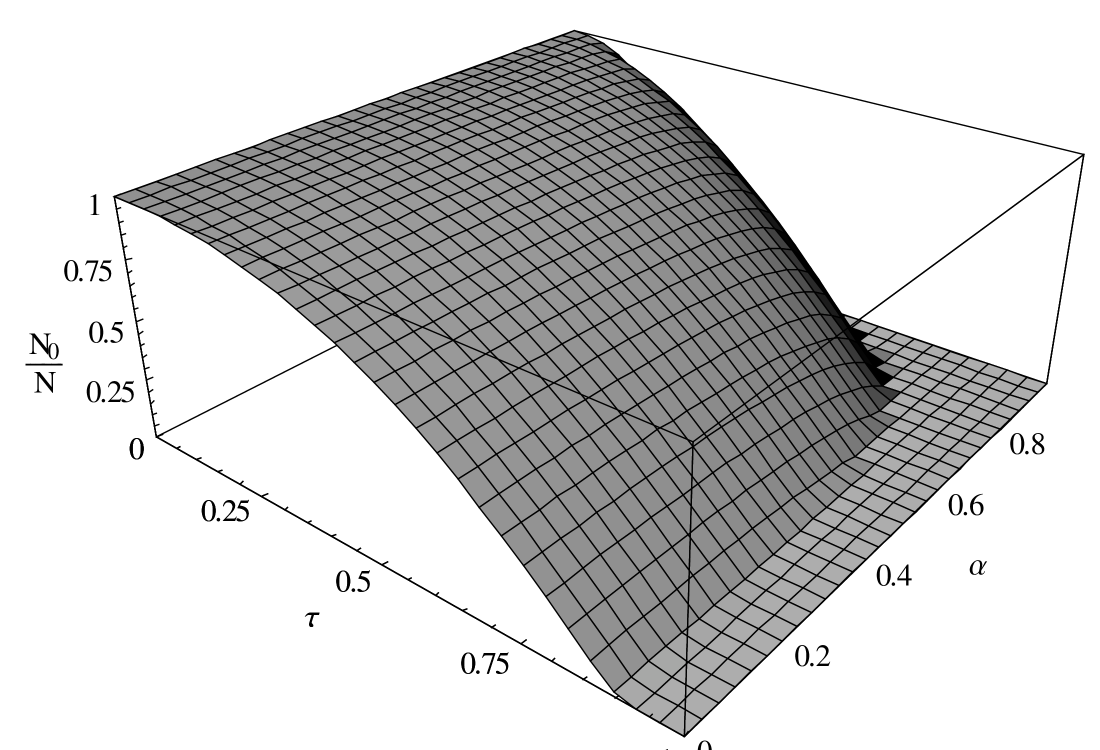
Figure 1: Condensate fraction versus the reduced temperature for different values of rotation rates $\alpha$ and $\eta=0.4$.

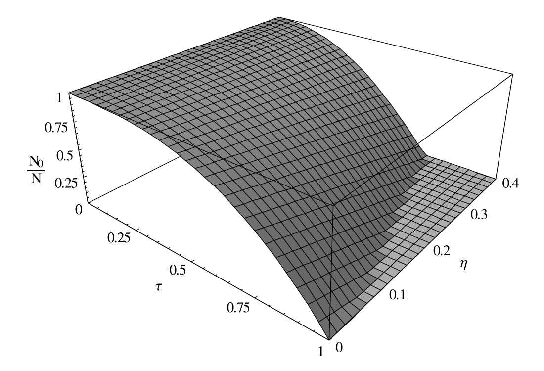
Figure 2: Condensate fraction versus the reduced temperature for different values of interaction parameter $\eta$ and rotation rate $\alpha=0.9$.

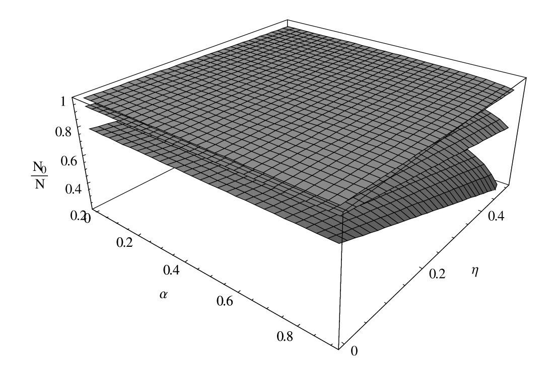
Figure 3: Condensate fraction versus the reduced temperature for different values of rotation rates $\alpha$ and interaction parameters $\eta$ for ${\cal T}=0.2,0.5$ and 0.8.

The second term in Eq.(34) leads to a reduction of the condensate fraction, as well as, it affected the transition temperature. This effect can be seen more clearly by calculating the critical temperature $T_{c}$. The latter is obtained as usual ket1 ; kir ; gro by setting $N_{0}/N$ in Eq.(34) equal to zero, thus

$$T_{c}=T_{0}[1-\frac{1}{3}K_{1}(\alpha)]$$ (38)

In the thermodynamic limit, the parameter $K_{1}(\alpha)$ vanishes and the critical temperature reduced to ideal Bose gas in a non-rotating frame $T_{0}$. Eq.(38) enabled us to investigate the effects of the rotation on $T_{c}(\Omega)$ in presence of the interatomic interaction. Indeed, in figure 4, the normalized critical temperature $(T_{c}(\Omega)/T_{0})$ is represented graphically as a function of rotation rate $\alpha$ and interaction effect $\eta$. This figure shows that the critical temperature $T_{c}$ decreases as compared with the non-interacting case due to the repulsive nature of the interaction.

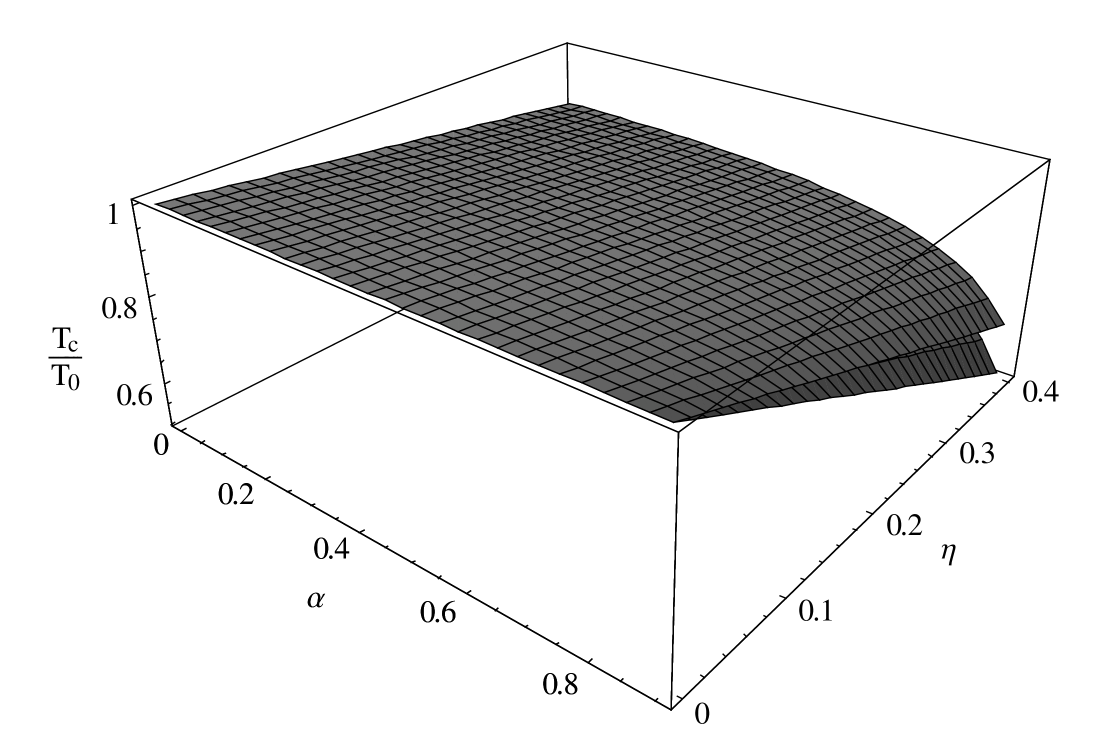
Figure 4: Critical temperature $T_{c}$, scaled by the non-rotating transition temperature $T_{0}$ for an interacting system, as a function of rotation rates $\alpha$.

IV.2 Entropy of the system

A major goal in the field of degenerate quantum gases is to reach a suitable very low temperature. Such low temperatures are necessary to reach phases relevant to condensed matter physics, such as quantum magnetism. However, to ascertain whether a given quantum phases is accessible, it is convenient to focus on its entropy, rather than temperature. Thus, it is important to determine and investigate the entropy-temperature curvesBlakie . The behavior of these curves is used in analyzing the process of adiabatic cooling Catani ; Schachenmayer ; Olf .

For the rotating condensate, the normalized entropy per particle is given by,

$$\frac{S}{Nk_{B}}=\frac{q}{N}+\frac{E}{Nk_{B}T}-\frac{\mu(\alpha)}{k_{B}T}$$ (39)

Following the usual procedure, the thermodynamic potential for one particle in terms of the normalized temperature ${\cal T}$ is

$$\frac{q}{N}=\frac{q_{0}}{N}+\frac{1}{\kappa_{+}\kappa_{-}}\frac{\zeta(4)}{\zeta(3)}{\cal T}^{3}+{\frac{\zeta(3)}{\zeta(2)}}K_{1}(\alpha){\cal T}^{2}$$ (40)

While in terms of the $q$-potential the total energy is given by $E=k_{B}T^{2}\ \Big{(}\frac{\partial q}{\partial T}\Big{)}_{\textsl{z}}$, thus

$$\frac{E}{Nk_{B}T}=\frac{E_{0}}{Nk_{B}T}+\frac{3}{\kappa_{+}\kappa_{-}}\frac{\zeta(4)}{\zeta(3)}{\cal T}^{3}+2{\frac{\zeta(3)}{\zeta(2)}}K_{1}(\alpha){\cal T}^{2}$$ (41)

Substituting from Eq’s.(40) and (41) in Eq.(39) we have,

$$\frac{S}{Nk_{B}}=\frac{S_{0}}{Nk_{B}}+\frac{4}{\kappa_{+}\kappa_{-}}\frac{\zeta(4)}{\zeta(3)}{\cal T}^{3}+{\frac{\zeta(3)}{\zeta(2)}}K_{1}(\alpha)\big{(}3{\cal T}^{2}-\frac{\kappa_{+}\kappa_{-}}{{\cal T}}\big{)}$$ (42)

where $S_{0}$ is the ground state entropy.

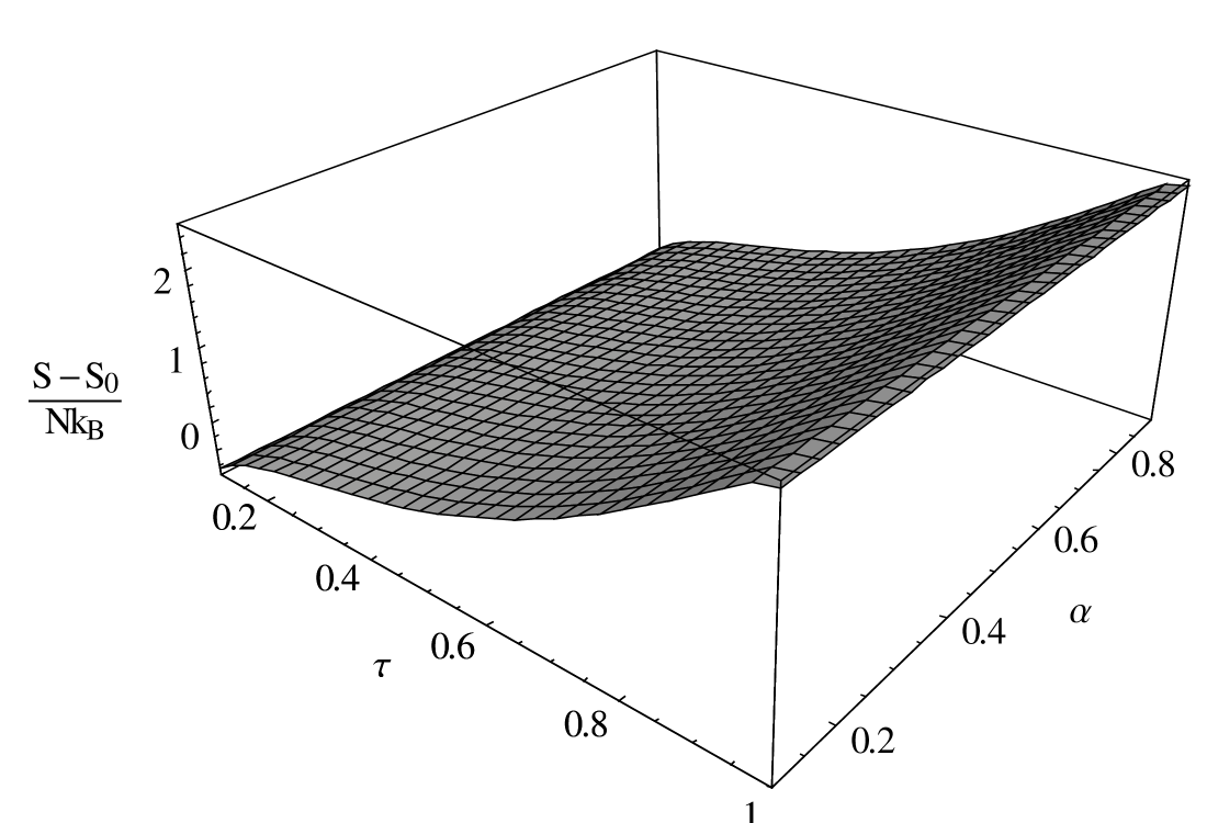
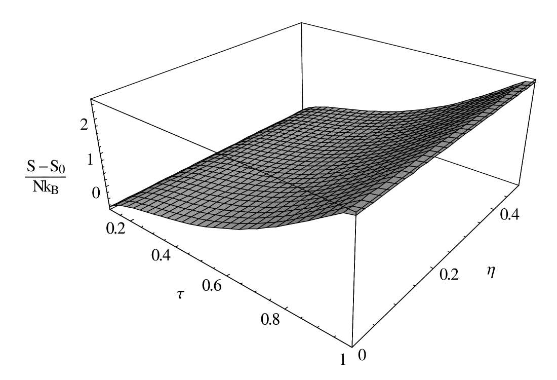
Figure 5: Entropy versus normalized temperature ${\cal T}$ with $\alpha$ and $\eta$ play as parameters.

In Fig(5), the entropy versus temperature curves as a function of $\alpha$ and $\eta$ are given. These figures show, as it is expected from standard thermodynamic arguments, that: as the temperature increases the entropy has a monotonically increasing nature everywhere. Consequently, in order to achieve thermal equilibrium in rotating frame, the trap should contain an asymmetry in the $xy-$plane. Even very small asymmetries are sufficient to ensure thermal equilibrium and safely calculation of the relevant thermodynamic parameters. However, one of the sensitive quantity to clear up the effects of the rotation and the interatomic interaction on the condensate is the behavior of the heat capacity as a function of the reduced temperature.

IV.3 Heat capacity

The essential features of BEC as a phase transition are clearly exhibited in the behavior of the specific heat, such as in the case of the $\lambda$ point superfluid transition of liquid helium, which is observed in its heat capacity.

The heat capacity per a particle at constant volume $\frac{C_{V}(T)}{Nk_{B}}$ is of considerable interest. It can be used as an indicator for the order of the phase transition and for the reduction of the system dimensionality.

In our approach,

$$C_{V}(T)=\Big{(}\frac{\partial E}{\partial\textsl{T}}\Big{)}_{N,V}=-\ \Big{(}\frac{\partial q}{\partial\beta}\Big{)}_{\textsl{z}},$$ (43)

However, it is known that for a given number of atoms, $C_{V}(T)$ increases to a maximum, then falls rapidly to a saturation value as $T$ increases greater than $T_{0}$. In such a situation, we must take into consideration two different temperature regimes, which are $T$ less or greater than $T_{0}$.

For ${\cal T}<1$, the heat capacity is given by

$$\frac{C_{V,{\cal T}<1}}{Nk_{B}}=\frac{1}{\kappa_{+}\kappa_{-}}\Big{\{}12{\cal T}^{3}\frac{\zeta(4)}{\zeta(3)}+6\ {K_{1}(\alpha)}{\cal T}^{2}\Big{\}}$$ (44)

While the heat capacity above ${\cal T}>1$ is given by

$$\frac{C_{V,{\cal T}>1}}{Nk_{B}} = \frac{1}{\kappa_{+}\kappa_{-}}\Big{\{}12\frac{\zeta(4)}{\zeta(3)}{\cal T}^{3}+6\ K_{1}(\alpha){\cal T}^{2}-\Big{[}3{\cal T}^{3}+$$ (45)

$$2 \frac{\zeta(2)}{\zeta(3)}K_{1}(\alpha){\cal T}^{2}\Big{]}\frac{3\zeta(3)+2K_{1}(\alpha)\zeta(2)/{\cal T}}{g_{2}(z)+K_{1}(\alpha)g_{1}(z)/{\cal T}}\Big{\}}$$

For non-rotating condensation, i.e. $\alpha=0$, the results previously obtained by Grossmann and Holthaus gro are recovered. While in the thermodynamic limit $N\to\infty(K_{1}=0)$, Eq’s.(44) and (45) are considerably simplify to,

$$\frac{C_{V,T<T_{0}}^{(\infty)}}{Nk_{B}}=\frac{12}{\kappa_{+}\kappa_{-}}\ \frac{\zeta(4)}{\zeta(3)}{\cal T}^{3}$$ (46)

$$\frac{C_{V,T>T_{0}}^{(\infty)}}{Nk_{B}}=\frac{3}{\kappa_{+}\kappa_{-}}\ \Big{[}4\ \frac{\zeta(4)}{g_{3}(z)}-3\ \frac{\zeta(3)}{g_{2}(z)}\Big{]}$$ (47)

Thus, at $T=T_{0}$ the heat capacity is discontinuous. The investigation of the heat capacity jump of a trapped gas near $T_{0}$ is important to understand the overall behavior of such phase transition; especially, for the non-homogeneous confinement case. However, the magnitude of the jump increases with the rotation rate according to $\frac{6.577}{\kappa_{+}\kappa_{-}}$. This discontinuity characterizes the phase transition to be of second order according to the Ehrenfest definition. This means that the system can be described by any potential of our choice. The choice then depends upon the thermodynamic variables you need, rather than upon the transition order. For completeness, in the case of the first order transition, the situation is basically the same. So, we can choose the potential whose variables are more suitable for us. The important difference only arises in the case when a limited portion of the system transforms into a new phase, while the rest of the body stays in the old one. Since we have simultaneously the jump of the solid volume and of the number of particles under the first order transition. So, we cannot fix the volume and the number of particles simultaneously. In this case, it is illegal to use the free energy or other potential whose variables are temperature, volume and the number of particles. We need, instead, to use the so-called thermodynamic-potential with the variables temperature, number of particles and the chemical potential.

Finally, one observes that the heat capacity Eq.(46) obeys the third law of thermodynamics which demands a vanishing of the heat capacity at zero temperature, and above $T_{0}$ is quite linear, in very good agreement with the standard theoretical result: $3k_{B}/N$ (corresponds to the Dulong-Petit law in the very high temperature limit). This interesting general shape of the heat capacity is accepted in the literaturegro ; sss ; Kling ; Jae .

The results calculated from Eq’s.(44) and (45) are represented in Fig.(6) and (7) for different values of $\alpha$ and $\eta$ respectively. The approximation used in pel is considered here to calculate Bose function $g_{l}(z)$ in Eq.(45).

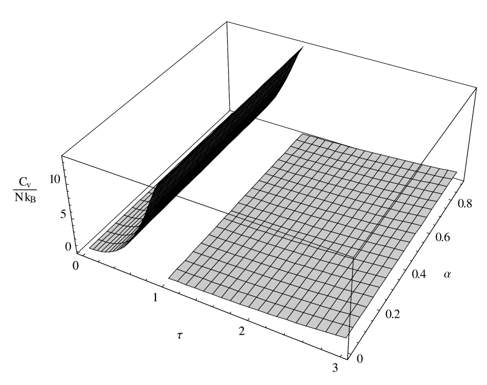
Figure 6: Variation of the heat capacity $C_{V}/Nk_{B}$ with the reduced temperature $T/T_{0}$ with $\alpha$ play as a parameter. The horizontal solid line corresponds to the Dulong-Petit law.

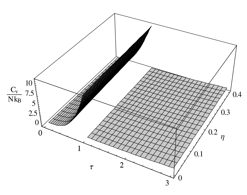
Figure 7: Variation of the heat capacity $C_{V}/Nk_{B}$ with the reduced temperature ${\cal T}$ with $\alpha$ play as a parameter, for $\eta=0.4.$

In Fig.6 and Fig.7, we plot the normalized heat capacity $C_{V}/Nk_{B}$ versus the normalized temperature, ${\cal T}$ with the rotation rate $\alpha$ and the interaction parameter $\eta$ plays as a parameter. The heat capacity evolves, starting from zero, with increasing values proportional to the third power of the normalized temperature, that is: $C_{V}\propto{\cal T}^{3}$. At ${\cal T}=1$ a steep jump takes place while it goes from ${\cal T}<1$ to ${\cal T}>1$. Right above the critical temperature, a slow decrease with the temperature is observed in $C_{V}$. And, at high temperatures, the heat capacity approaches the temperature independent behavior expected for the non-interacting Bose gas: $3Nk_{B}$.

It is interesting to note that signatures of a phase transition appear in the specific heat behavior as a function of ${\cal T},\alpha$ and $\eta$. As T decreases, the phase transition, observed at ${\cal T}=1$, reveals the transition from noncondensed state to those which is in condensed phase.

V Conclusion

In conclusion, by employing the semiclassical Hartree-Fock approximation, we obtain the analytical expression of the thermodynamic potential of a rotating interacting Bose gas in an anisotropic harmonic trap. Then, the expressions for the condensate fraction: transition temperature, entropy and the specific heat are derived. The calculated results showed that these thermodynamic quantities depend on the rotation rate as well as the interatomic interaction for all temperature range. The critical temperature and the condensate fraction are decreasing compared with the ideal Bose gas case. Using $C_{v}$ as the indicator, we also investigated the phase transition from the gas phase to condensed phase. The method we have outlined here can be extended to study and investigate the thermodynamic properties of a rotating boson gas in the presence of a combined harmonic lattice potential.

References

- (1) K. Madison, F. Chevy, W. Wohlleben, and J. Dalibard, Phys. Rev. Lett 84 (2000) 806.
- (2) M. R. Matthews, B. P. Anderson, P. C. Haljan, D. S. Hall, C. E. Wieman, and E. A. Cornell Phys. Rev. Lett. 83 (1999) 2498.
- (3) I. Coddington, P. C. Haljan, P. Engels, V. Schweikhard, S. Tung and E. A. Cornell, Phys. Rev. A 70 (2004) 063607.
- (4) F. Dalfovo, S. Giorgini, L.P. Pitaevskii and S. Stringari, Rev. of Mod. Phys. 71 (1999) 463.
- (5) S. Giorgini, L. P. Pitaevskii, and S. Stringari, Journal of Low Temperature Physics 109 (1997) 309.
- (6) N. Tammuz, Thermodynamics of ultracold atomic Bose gases with tuneable interactions (Ph.D. thesis, Cavendish Laboratory, University of Cambridge, UK, 2011).
- (7) S. Stringari, Phys. Rev. Lett 82 (1999) 4371; Phys. Rev. Lett 86 (2001) 4725.
- (8) S. Stock,Quantized Vortices in a Bose-Einstein Condensate:Thermal Activation and Dynamic Nucleation, PhD thesis, Université Paris 6, France, January (2006) ch. 9.
- (9) N. van Druten and W. Ketterle, Phys. Lett. Lett. 79 (1997) 549.
- (10) R. F. Shiozaki, G. D. Telles, P. Castilho, F. J. Poveda Cuevas, S. R. Muniz, G. Roati, V. Romero-Rochin, and V. S. Bagnato, Phys. Rev. A 90 (2014) 043640.
- (11) R. Olf, F. Fang, G. E. Marti, A. MacRae, and D. M. Stamper-Kurn, Nature Physics 11 (2015) 720.
- (12) S. Kling and A. Pelster, Phys. Rev. A 76 (2007) 023609.
- (13) A. L. Fetter, Phys. Rev. A 64 (2001) 063608; Physica C 404 (2004) 158; Rev. Mod. Phys. 81 (2009) 647.
- (14) Y. Li, and Q. Gu, Phys. Lett. A 378 (2014) 1233; F. Jing-Han, G. Qiang, G. Wei, Chin. Phys. Lett. 28 (2011) 060306; Y. X. Chen, J. H. Qin, Q. Gu, Phys. Lett. A 378 (2014) 421; X. L. Jian, J. H. Qin, Q. Gu, J. Phys. Condens. Matter 23 (2011) 026003.
- (15) S. Sinha, Phys. Rev. A 58 (1998) 3159.
- (16) N. Sandoval-Figueroa and V. Romero-Rochin, Phys. Rev. E 78 (2008) 061129.
- (17) J. G. Kim and E. K. Lee, J. Phys. B: At. Mol. Opt. Phys. 32 (1999) 5575.
- (18) S. Bargi, G. M. Kavoulakis, and S. M. Reimann, Phys.Rev. A 73 (2006) 033613.
- (19) L. Pitaevskii and S. Stringari, Bose-Einstein condensation condensation, Clarendon Press. Oxford (2003) chapter 14.
- (20) N. R. Cooper, Adv. Phys 57 (2008) 539.
- (21) Pathria R K , Statistical Mechanics, (Pergammon, London ,1972).
- (22) K. Kirsten, and D. J. Toms, Phys. Lett. A, 222 (1996) 148 ; K. Kirsten, and D. J. Toms, Phys. Rev. A 54 (1996) 4188; K. Kirsten, and D. J. Toms, Phys. Lett. A, 243 (1998) 137; K. Kirsten, and D. J. Toms, Phys. Rev. E, 59 (1999) 158.
- (23) H. Haugerud, T. Haugset, and F. Ravndal, Phys. Lett. A 225 (1997) 18.
- (24) V. Bretin, S. Stock, Y. Seurin, and J. Dalibard, Phys. Rev. Lett. 92 (2004) 050403.
- (25) R. Campbell, Thermodynamic properties of a Bose gas with tuneable interactions (Ph.D. thesis, Cavendish Laboratory, University of Cambridge, UK, 2011).
- (26) M. Naraschewski, D. M. Stamper-Kurn, Phys. Rev. A 58 (1998) 2423.
- (27) S. Grossmann, S. and M. Holthaus, Phys. Lett. A 208 (1995) 188.
- (28) S. Stock, B. Battelier, V. Bretin, Z. Hadzibabic, J. Dalibard, Laser Physics Letters 2 (2005) 275; A. Aftalion, X. Blanc, and J. Dalibard, Phys. Rev. A 71 (2005) 023611.
- (29) A. S. Hassan and A. M. El-Badry, Eur. Phys. J. D 68 (2014) 76.
- (30) A. S. Hassan, A. M. El-Badry, and S. S. M. Soliman, Eur. Phys. J. D 64 (2011) 465.
- (31) A. S. Hassan, Phys. Lett. A 374 (2010) 2106.
- (32) A. S. Hassan, A. M. El-Badry, and S. S. M. Soliman, Physica B 405 (2010) 4768.
- (33) G. Su, L. Chen, and J. Chen, Phys. Lett. A 326 (2004) 252.
- (34) M. Linn and A. L. Fetter, Phys. Rev. A 60, (1999) 4910.
- (35) S. Giorgini and L.P. Pitaevskii and S. Stringari, Phys. Rev. Lett. 78 (1997) 3987.
- (36) R. L. D. Campbell, R. P. Smith, N. Tammuz, S. Beattie, S. Moulder, and Z. Hadzibabic, Phys. Rev. A 82 (2010) 063611.
- (37) N. Tammuz, R. P. Smith, R. L. D. Campbell, S. Beattie, S. Moulder, J. Dalibard, and Z. Hadzibabic, Phys. Rev. Lett. 106 (2011) 230401.
- (38) R. P. Smith, R. L. D. Campbell, N. Tammuz, and Z. Hadzibabic, Phys. Rev. Lett. 106 (2011) 250403.
- (39) R. P. Smith, N. Tammuz, R. L. D. Campbell, M. Holzmann, and Z. Hadzibabic, Phys. Rev. Lett. 107 (2011) 190403.
- (40) P. B. Blakie and J. V. Porto, Phys. Lett. A 69 (2004) 013603.
- (41) J. Catani, G. Barontini, G. Lamporesi, F. Rabatti, G. Thalhammer, F. Minardi, S. Stringari, and M. Inguscio, Phys. Lett. A 103 (2009) 140401.
- (42) J. Schachenmayer, D. M. Weld, H. Miyake, G. A. Siviloglou, W. Ketterle, and A. J. Daley, Phys. Rev. A 92, (2015) 041602.
- (43) B. Klünder, and A. Pelster, Eur. Phys. J. B 68 (2009) 457.