Convergence Rates of Inertial Splitting Schemes for Nonconvex Composite Optimization

Abstract

We study the convergence properties of a general inertial first-order proximal splitting algorithm for solving nonconvex nonsmooth optimization problems. Using the Kurdyka–Łojaziewicz (KL) inequality we establish new convergence rates which apply to several inertial algorithms in the literature. Our basic assumption is that the objective function is semialgebraic, which lends our results broad applicability in the fields of signal processing and machine learning. The convergence rates depend on the exponent of the “desingularizing function” arising in the KL inequality. Depending on this exponent, convergence may be finite, linear, or sublinear and of the form $O(k^{-p})$ for $p>1$.

Index Terms—  Kurdyka–Łojaziewicz Inequality, Inertial forward-backward splitting, heavy-ball method, convergence rate, first-order methods.

1 Introduction

We are interested in solving the following optimization problem

$$\min_{x\in\mathbb{R}^{n}}\Phi(x)=f(x)+g(x)$$ (1)

where $g:\mathbb{R}^{n}\to\mathbb{R}\cup\{+\infty\}$ is lower semicontinuous (l.s.c.) and $f:\mathbb{R}^{n}\to\mathbb{R}$ is differentiable with Lipschitz continuous gradient. We also assume that $\Phi$ is semialgebraic [1], meaning there integers $p,q\geq 0$ and polynomial functions $P_{ij},Q_{ij}:\mathbb{R}^{n+1}\to\mathbb{R}$ such that

$$\{(x,y):y\geq f(x)\}=\underset{j=1}{\overset{p}{\cup}}\underset{i=1}{\overset{q}{\cap}}\{z\in\mathbb{R}^{n+1}:P_{ij}(z)=0,Q_{ij}(z)<0\}.$$

We make no assumption of convexity. Semialgebraic objective functions in the form of (1) are widespread in machine learning, image processing, compressed sensing, matrix completion, and computer vision [2, 3, 4, 5, 6, 7, 8]. We will list a few examples below.

In this paper we focus on the application of Prob. (1) to sparse least-squares and regression. This problem arises when looking for a sparse solution to a set of underdetermined linear equations. Such problems occur in compressed sensing, computer vision, machine learning and many other related fields. Suppose we observe $y=Ax+b$ where $b$ is noise and wish to recover $x$ which is known to be sparse, however the matrix $A$ is “fat” or poorly conditioned. One approach is to solve (1) with $f$ a loss function modeling the noise $b$ and $g$ a regularizer modeling prior knowledge of $x$, in this case sparsity. The correct choice for $f$ will depend on the noise model and may be nonconvex. Examples of appropriate nonconvex semialgebraic choices for $g$ are the $\ell_{0}$ pseudo-norm, and the smoothly clipped absolute deviation (SCAD) [9]. The prevailing convex choice is the $\ell_{1}$ norm which is also semialgebraic. SCAD has the advantage over the $\ell_{1}$-norm that it leads to nearly unbiased estimates of large coefficients [9]. Furthermore unlike the $\ell_{0}$ norm SCAD leads to a solution which is continuous in the data matrix $A$. Nevertheless $\ell_{1}$-based methods continue to be the standard throughout the literature due to convexity and computational simplicity.

For Problem (1), first-order methods have been found to be computationally inexpensive, simple to implement, and effective solvers [10]. In this paper we are interested in first order methods of the inertial type, also known as momentum methods. These methods generate the next iterate using more than one previous iterate so as to mimic the inertial dynamics of a model differential equation. In many instances both in theory and in practice, inertial methods have been shown to converge faster than noninertial ones [11]. Furthermore for nonconvex problems it has been observed that using inertia can help the algorithm escape local minima and saddle points that would capture other first-order algorithms [12, Sec 4.1]. A prominent example of the use of inertia in nonconvex optimization is training neural networks, which goes under the name of back propagation with momentum [13]. In convex optimization a prominent example is the heavy ball method [11].

Over the past decade the KL inequality has come to prominence in the optimization community as a powerful tool for studying both convex and nonconvex problems. It is very general, applicable to almost all problems encountered in real applications, and powerful because it allows researchers to precisely understand the local convergence properties of first-order methods. The inequality goes back to [14, 15]. In [16, 17, 18] the KL inequality was used to derive convergence rates of descent-type first order methods. The KL inequality was used to study convex optimization problems in [19, 20].

Nonconvex optimization has traditionally been challenging for researchers to study since generally they cannot distinguish a local minimum from a global minimum. Nevertheless, for some applications such as empirical risk minimization in machine learning, finding a good local minimum is all that is required of the optimization solver [21, Sec. 3]. In other problems local minima have been shown to be global minima [22].

Contributions: The main contribution of this paper is to determine for the first time the local convergence rate of a broad family of inertial proximal splitting methods for solving Prob. (1). The family of methods we study includes several algorithms proposed in the literature for which convergence rates are unknown. The family was proposed in [23], where it was proved that the iterates converge to a critical point. However the convergence rate, e.g. how fast the iterates converge, was not determined. In fact in [23], local linear convergence was shown under a partial smoothness assumption. In contrast we do not assume partial smoothness and our results are far more general. We use the KL inequality and show finite, linear, or sublinear convergence, depending on the KL exponent (see Sec. 2). The main inspiration for our work is [18] which studied convergence rates of several noninertial schemes using the KL property. However, the analysis of [18] cannot be applied to inertial methods. Our approach is to extend the framework of [18] to the inertial setting. This is done by proving convergence rates of a multistep Lyapunov potential function which upper bounds the objective function. We also prove convergence rates of the iterates and extend a result of [20, Thm. 3.7 ] to show that our multistep Lyapunov potential has the same KL exponent as the objective function. Finally we include experiments to illustrate the derived convergence rates.

Notation: Given a closed set $C$ and point $x$, define $d(x,C)\triangleq\min\{\|x-c\|:c\in C\}$. For a sequence $\{x_{k}\}_{k\in\mathbb{N}}$ let $\Delta_{k}\triangleq\|x_{k}-x_{k-1}\|$. We say that $x_{k}\to x^{*}$ linearly with convergence factor $q\in(0,1)$ if there exists $C>0$ such that $\|x_{k}-x^{*}\|\leq Cq^{k}$.

2 Mathematical Background

In this section we give an overview of the relevant mathematical concepts. We use the notion of the limiting subdifferential $\partial\Phi(x)$ of a l.s.c. function $\Phi$. For the definition and properties we refer to [1, Sec 2.1]. A necessary (but not sufficient) condition for $x$ to be a minimizer of $\Phi$ is $0\in\partial\Phi(x)$. The set of critical points of $\Phi$ is $\text{crit}(\Phi)\triangleq\{x:0\in\partial\Phi(x)\}$. A useful notion is the proximal operator w.r.t. a l.s.c. proper function $g$, defined as

$${\text{prox}}_{g}(x)=\underset{x^{\prime}\in\mathbb{R}^{n}}{\arg\min}\,\,\,g(x^{\prime})+\frac{1}{2}\|x-x^{\prime}\|^{2},$$

which is always nonempty. Note that, unlike the convex case, this operator is not necessarily single-valued.

• A function $f:\mathbb{R}^{n}\to\overline{\mathbb{R}}$ is said to have the Kurdyka-Lojasiewicz (KL) property at $x^{*}\in\text{dom}\,\partial f$ if there exists $\eta\in(0,+\infty]$, a neighborhood $U$ of $x^{*}$, and a continuous and concave function $\varphi:[0,\eta)\to\mathbb{R}_{+}$ such that

  1. $\varphi(0)=0$,

  2. $\varphi$ is $C^{1}$ on $(0,\eta)$ and for all $s\in(0,\eta)$, $\varphi^{\prime}(s)>0$,

  3. for all $x\in U\cap\{x:f(x^{*})<f(x)<f(x^{*})+\eta\}$ the KL inequality holds:

     $$\varphi^{\prime}(f(x)-f(x^{*}))d(0,\partial f(x))\geq 1.$$ (2)

  If $f$ is semialgebraic, then it has the KL property at all points in $\text{dom}\,\partial f$, and $\varphi(t)=\frac{c}{\theta}t^{\theta}$ for $\theta\in(0,1]$.

In the semialgebraic case we will refer to $\theta$ as the KL exponent (note that some other papers use $1-\theta$ [20]). For the special case where $f$ is smooth, (2) can be rewritten as $\|\nabla(\varphi\circ(f(x)-f(x^{*}))\|\geq 1,$ which shows why $\varphi$ is called a “desingularizing function”. The slope of $\varphi$ near the origin encodes information about the “flatness” of the function about a point, thus the KL exponent provides a way to quantify convergence rates of iterative first-order methods.

For example the 1D function $f(x)=|x|^{p}$ for $p\geq 2$ has desingluarizing function $\varphi(t)=t^{\frac{1}{p}}$. The larger $p$, the flatter $f$ is around the origin, and the slower gradient-based methods will converge. In general, functions with smaller exponent $\theta$ have slower convergence near a critical point [18]. Thus, determining the KL exponent of an objective function holds the key to assessing convergence rates near critical points. Note that for most prominent optimization problems, determining the KL exponent is an open problem. Nevertheless many important examples have been determined recently, such as least-squares and logistic regression with an $\ell_{1}$, $\ell_{0}$, or SCAD penalty [20]. A very interesting recent work showed that for convex functions the KL property is equivalent to an error bound condition which is often easier to check in practice [19].

We now precisely state our assumptions on Problem (1), which will be in effect throughout the rest of the paper.

Assumption 1. The function $\Phi:\mathbb{R}^{n}\to\mathbb{R}\cup\{+\infty\}$ is semialgebraic, bounded from below, and has desingularizing function $\varphi(t)=\frac{c}{\theta}t^{\theta}$ where $c>0$ and $\theta\in(0,1]$. The function $g:\mathbb{R}^{n}\to\overline{\mathbb{R}}$ is l.s.c., and $f:\mathbb{R}^{n}\to\mathbb{R}$ has Lipschitz continuous gradient with constant $L$.

3 A Family of Inertial Algorithms

We study the family of inertial algorithms proposed in [23]. In what follows $s\geq 1$ is an integer, and $I=\{0,1,\ldots,s-1\}$.

Algorithm 1 Multi-step Inertial Forward-Backward splitting (MiFB)

0:  $x_{0}\in\mathbb{R}^{n}$, $0<\underline{\gamma}\leq\overline{\gamma}<1/L$.

  Set $x_{-s}=\ldots=x_{-1}=x_{0}$, $k=1$

  repeat

     Choose $0<\underline{\gamma}\leq\gamma_{k}\leq\overline{\gamma}<1/L$, $\{a_{k,0},a_{k,1},\ldots\}\in(-1,1]^{s}$, $\{b_{k,0},b_{k,1},\ldots\}\in(-1,1]^{s}$.

     $y_{a,k}=x_{k}+\sum_{i\in I}a_{k,i}(x_{k-i}-x_{k-i-1})$

     $y_{b,k}=x_{k}+\sum_{i\in I}b_{k,i}(x_{k-i}-x_{k-i-1})$

     $x_{k+1}\in{\text{prox}}_{\gamma_{k}g}\left(y_{a,k}-\gamma_{k}\nabla f(y_{b,k})\right)$

     $k=k+1$

  until convergence

Note the algorithm as stated leaves open the choice of the parameters $\{a_{k,i},b_{k,i},\gamma_{k}\}$. For convergence conditions on the parameters we refer to Section 4 and [24, Thm. 1].

The algorithm is very general and covers several inertial algorithms proposed in the literature as special cases. For instance the inertial forward-backward method proposed in [12] corresponds to MiFB with $s=1$, and $b_{k,0}=0$. The well-known iPiano algorithm also corresponds to this same parameter choice, however the original analysis of this algorithm assumed $g$ was convex [25]. The heavy-ball method is an early and prominent inertial first-order method which also corresponds to this parameter choice when $g=0$. The heavy-ball method was originally proposed for strongly convex quadratic problems but was considered in the context of nonconvex problems in [26]. The analysis of [27] applies to MiFB for the special case when $s=1$ and $a_{k,0}=b_{k,0}$. However [27] only derived convergence rates of the iterates and not the function values, which are our main interest. Furthermore [27] used a different proof technique to the one used here. This same parameter choice has been considered for convex optimization in [24, 28], albeit without the sharp convergence rates derived here. In both the convex and nonconvex settings, employing inertia has been found to improve either the convergence rate or the quality of the obtained local minimum in several studies [12, 25, 23, 24].

General convergence rates have not been derived for MiFB under nonconvexity and semialgebraicity assumptions. The convergence rate of iPiano has been examined in a limited situation where the KL exponent $\theta=1/2$ in [20, Thm 5.2]. Note that the primary motivation for studying this framework is its generality - allowing our analysis to cover many special cases from the literature. However the case $s=1$ is the most interesting in practice and corresponds to the most prominent inertial algorithms.

4 Convergence Rate Analysis

Throughout the analysis, Assumption 1 is in effect. Before providing our convergence rate analysis, we need a few results from [23].

Theorem 1.

Fix $s\geq 1$ and recall $I=\{0,1,\ldots,s-1\}$. Fix $\{\gamma_{k}\}$, $\{a_{k,i}\}$ and $\{b_{k,i}\}$ for $k\in\mathbb{N}$ and $i\in I$. Fix $\mu,\nu>0$ and define

$$\beta_{k} \triangleq \frac{1-\gamma_{k}L-\mu-\nu\gamma_{k}}{2\gamma_{k}},\quad\underline{\beta}\triangleq\underset{k\in\mathbb{N}}{\lim\inf}\,\beta_{k},$$

$$\alpha_{k,i} \triangleq \frac{sa_{k,i}^{2}}{2\gamma_{k}\mu}+\frac{sb_{k,i}^{2}L^{2}}{2\nu},\quad\overline{\alpha}_{i}\triangleq\underset{k\in\mathbb{N}}{\lim\sup}\,\alpha_{k,i},$$

and $z_{k}\triangleq(x_{k}^{\top},x_{k-1}^{\top},\ldots,x_{k-s}^{\top})^{\top}$. Define the multi-step Lyapunov function as

$$\Psi(z_{k})\triangleq\Phi(x_{k})+\sum_{i\in I}\left(\sum_{j=i}^{s-1}\overline{\alpha}_{j}\right)\Delta_{k-i}^{2}.$$ (3)

and

$$\delta\triangleq\underline{\beta}-\sum_{i\in I}\overline{\alpha}_{i}>0.$$ (4)

If the parameters are chosen so that $\delta>0$ then

1. for all $k$, $\Psi(z_{k+1})\leq\Psi(z_{k})-\delta\Delta_{k+1}^{2}$,

2. for all $k$, there is a $\sigma>0$ such that $d(0,\partial\Psi(z_{k}))\leq\sigma\sum_{j=k+1-s}^{k}\Delta_{j}$,

3. If $\{x_{k}\}$ is bounded there exists $x^{*}\in\text{crit}(\Phi)$ such that $x_{k}\to x^{*}$ and $\Phi(x_{k})\to\Phi(x^{*})$.

Proof.

Statements (i) and (ii) are shown in [23, Lemma A.5] and [23, Fact (R.2)] respectively. The fact that $\Phi(x_{k})\to\Phi(x^{*})$ is shown in [23, Lemma A.6]. The fact that $x_{k}\to x^{*}$ is the main result of [23, Thm 2.2].

The assumption that $\{x_{k}\}$ is bounded is standard in the analysis of algorithms for nonconvex optimization and is guaranteed under ordinary conditions such as coercivity. Since the set of semialgebraic functions is closed under addition, $\Psi$ is semialgebraic [29]. We now give our convergence result.

Theorem 2.

Assume the parameters of MiFB are chosen such that $\delta>0$ where $\delta$ is defined in (4), thus there exists a critical point $x^{*}$ such that $x_{k}\to x^{*}$. Let $\theta$ be the KL exponent of $\Psi$ defined in (3).

1. If $\theta=1$, then $x_{k}$ converges to $x^{*}$ in a finite number of iterations.

2. If $\frac{1}{2}\leq\theta<1$, then $\Phi(x_{k})\to\Phi(x^{*})$ linearly.

3. If $0<\theta<1/2$, then $\Phi(x_{k})-\Phi(x^{*})=O\left(k^{\frac{1}{2\theta-1}}\right)$.

Proof.

The starting point is the KL inequality applied to the multi-step Lyapunov function defined in (3). Let $z^{*}\triangleq((x^{*})^{\top},\ldots,(x^{*})^{\top})^{\top}$. Suppose $\Psi(z_{K})=\Psi(z^{*})$ for some $K>0$. Then the descent property of Thm. 1(i), along with the fact that $\Psi(z_{k})\to\Psi(z^{*})$, implies that $\Delta_{K+1}=0$ and therefore $\Psi(z_{k})=\Psi(z^{*})$ holds for all $k>K$. Therefore assume $\Psi(z_{k})>\Psi(z^{*})$. Now since $z_{k}\to z^{*}$ and $\Psi(z_{k})\to\Psi(z^{*})$, there exists $k_{0}>0$ such that for $k>k_{0}$ (2) holds with $f=\Psi$. Assume $k>k_{0}$. Squaring both sides of (2) yields

$$\varphi^{\prime 2}(\Psi(z_{k})-\Psi(z^{*}))d(0,\partial\Psi(z_{k}))^{2}\geq 1,$$ (5)

Now substituting Thm.1 (ii) into (5) yields

$$\sigma^{2}\varphi^{\prime 2}(\Psi(z_{k})-\Psi(z^{*}))\left(\sum_{j=k+1-s}^{k}\Delta_{j}\right)^{2}\geq 1.$$ (6)

Now

$$\left(\sum_{j=k+1-s}^{k}\Delta_{j}\right)^{2} \leq s\sum_{j=k+1-s}^{k}\Delta_{j}^{2}$$

$$\leq \frac{s}{\delta}\sum_{j=k+1-s}^{k}\left(\Psi(z_{j-1})-\Psi(z_{j})\right)$$

$$= \frac{s}{\delta}\left(\Psi(z_{k-s})-\Psi(z_{k})\right),$$

where in the first inequality we have used the fact that $(\sum_{i=1}^{s}a_{i})^{2}\leq s\sum_{i=1}^{n}a_{i}^{2}$, and in the second inequality we have used Thm. 1(i). Substituting this into (6) yields

$$\frac{\sigma^{2}s}{\delta}\varphi^{\prime 2}(\Psi(z_{k})-\Psi(z^{*}))\left(\Psi(z_{k-s})-\Psi(z_{k})\right)\geq 1,$$

from which convergence rates can be derived by extending the arguments in [18, Thm 4].

Proceeding, let $r_{k}\triangleq\Psi(z_{k})-\Psi(z^{*})$, and $C_{1}\triangleq\frac{\delta}{\sigma^{2}c^{2}s}$, then using $\varphi^{\prime}(t)=ct^{\theta-1}$, we get

$$r_{k-s}-r_{k}\geq C_{1}r_{k}^{2(1-\theta)}.$$ (7)

If $\theta=1$, then the recursion becomes $r_{k-s}-r_{k}\geq C_{1},\quad\forall k>k_{0}.$ Since by Theorem 1 (iii), $r_{k}$ converges, this would require $C_{1}=0$, which is a contradiction. Therefore there exists $k_{1}$ such that $r_{k}=0$ for all $k>k_{1}$.

Suppose $\theta\geq 1/2$, then since $r_{k}\to 0$, there exists $k_{2}$ such that for all $k>k_{2}$, $r_{k}\leq 1$, and $r_{k}^{2(1-\theta)}\geq r_{k}$. Therefore for all $k>k_{2}$,

$$r_{k-s}-r_{k}\geq C_{1}r_{k}\implies r_{k} \leq (1+C_{1})^{-1}r_{k-s}$$ (8)

$$\leq (1+C_{1})^{-p_{1}}r_{k_{2}},$$

where $p_{1}\triangleq\lfloor\frac{k-k_{2}}{s}\rfloor$ Note that $p_{1}>\frac{k-k_{2}-s}{s}$. Therefore $r_{k}\to 0$ linearly. Note that if $\theta=\frac{1}{2}$, $2(1-\theta)=1$ and (8) holds for all $k\geq k_{0}$.

Finally suppose $\theta<1/2$. Define $\phi(t)\triangleq\frac{D}{1-2\theta}t^{2\theta-1}$ where $D>0$, so $\phi^{\prime}(t)=-Dt^{2\theta-2}$. Now

$$\phi(r_{k})-\phi(r_{k-s})=\int_{r_{k-s}}^{r_{k}}\phi^{\prime}(t)dt = D\int^{r_{k-s}}_{r_{k}}t^{2\theta-2}dt.$$

Therefore since $r_{k-s}\geq r_{k}$ and $t^{2\theta-2}$ is nonincreasing,

$$\phi(r_{k})-\phi(r_{k-s})\geq D(r_{k-s}-r_{k})r_{k-s}^{2\theta-2}.$$

Now we consider two cases.

Case 1: suppose $2r_{k-s}^{2\theta-2}\geq r_{k}^{2\theta-2}$, then

$$\phi(r_{k})-\phi(r_{k-s})\geq\frac{D}{2}(r_{k-s}-r_{k})r_{k}^{2\theta-2}\geq\frac{C_{1}D}{2}.$$ (9)

where in the second inequality we have used (7).

Case 2: suppose that $2r_{k-s}^{2\theta-2}<r_{k}^{2\theta-2}$. Now $2\theta-2<2\theta-1<0$, therefore $(2\theta-1)/(2\theta-2)>0$, thus $r_{k}^{2\theta-1}>qr_{k-s}^{2\theta-1}$ where $q=2^{\frac{2\theta-1}{2\theta-2}}>1$. Thus

$$\phi(r_{k})-\phi(r_{k-s}) = \frac{D}{1-2\theta}\left(r_{k}^{2\theta-1}-r_{k-s}^{2\theta-1}\right)$$ (10)

$$> \frac{D}{1-2\theta}(q-1)r_{k-s}^{2\theta-1}$$

$$\geq \frac{D}{1-2\theta}(q-1)r_{k_{0}}^{2\theta-1}\triangleq C_{2}.$$

Thus putting together (9) and (10) yields $\phi(r_{k})\geq\phi(r_{k-s})+C_{3}$ where $C_{3}=\max(C_{2},\frac{C_{1}D}{2})$. Therefore

$$\phi(r_{k}) \geq \phi(r_{k})-\phi(r_{k-p_{2}s})\geq p_{2}C_{3}$$

where $p_{2}\triangleq\lfloor\frac{k-k_{0}}{s}\rfloor$. Therefore

$$r_{k}\leq\left(\frac{1-2\theta}{D}\right)^{\frac{1}{2\theta-1}}{(p_{2}C_{3})}^{\frac{1}{2\theta-1}}\leq C_{4}\left(\frac{k-s-k_{0}}{s}\right)^{\frac{1}{2\theta-1}}.$$

where $C_{4}=\left(\frac{C_{3}(1-2\theta)}{D}\right)^{\frac{1}{2\theta-1}}$. To end the proof, note that $\Phi(x_{k})\leq\Psi(z_{k})$.

In the case where $f$ and $g$ are also convex, we can use parameter choices specified in [24, Thm. 1].

5 Convergence Rates of the Iterates

The convergence rates of $\|x_{k}-x^{*}\|$ can also be quantified. To do so we need another result from [23].

Lemma 3.

Recall the notation $r_{k}\triangleq\Psi(z_{k})-\Psi(z^{*})$. Let $\epsilon_{k}\triangleq\frac{\sigma}{\delta}\left(\varphi(r_{k})-\varphi(r_{k+1})\right)$ where $\sigma$ is defined in Theorem 1 (ii) and $\delta$ in (4). Fix $\kappa>0$ so that $\kappa<2/s$. Assume the parameters of MiFB are chosen to so that $\delta>0$ and $\{x_{k}\}$ is bounded. Then there exists a $k_{0}>0$ such that for all $k>k_{0}$

$$r_{k}>0\implies\Delta_{k}\leq\frac{\kappa}{2}\sum_{j=k-s}^{k-1}\Delta_{j}+\frac{1}{2\kappa}\epsilon_{k-1}.$$ (11)

Proof.

This inequality is proved on page 14 of [23] as part of the proof of [23, Thm 2.2].

We now state our result.

Theorem 4.

Assume $\{x_{k}\}$ is bounded and the parameters of MiFB are chosen so that $\delta>0$ where $\delta$ is defined in (4). Let $\theta$ be the KL exponent of $\Psi$ defined in (3). Then

1. If $\theta=1$, then $x_{k}=x^{*}$ after finitely many iterations.

2. If $\frac{1}{2}\leq\theta<1$, $x_{k}\to x^{*}$ linearly.

3. If $0<\theta<\frac{1}{2}$, $\|x_{k}-x^{*}\|=O\left(k^{\frac{\theta}{2\theta-1}}\right)$.

Proof.

Statement (a) follows trivially from the fact that $r_{k}=0$ after finitely many iterations, and therefore $\Delta_{k}=0$. We proceed to prove statements (b) and (c). As with Theorem 2 the basic idea is to extend the techniques of [18] to allow for the inertial nature of the algorithm. The starting point is (11). Fix $K>k_{0}$. Then

$$\sum_{k\geq K}\Delta_{k} \leq \frac{\kappa}{2}\sum_{k\geq K}\sum_{j=k-s}^{k-1}\Delta_{j}+\frac{1}{2\kappa}\sum_{k\geq K}\epsilon_{k-1}$$

$$\leq \frac{\kappa s}{2}\sum_{k\geq K-s}\Delta_{k}+\frac{1}{2\kappa}\sum_{k\geq K}\epsilon_{k-1}$$

Let $C=\frac{\kappa s}{2}$ and note that $0<C<1$. Therefore subtracting $C\sum_{k\geq K}\Delta_{k}$ from both sides yields

$$\sum_{k\geq K}\Delta_{k}\leq\frac{1}{1-C}\left(C\sum_{k=K-s}^{K-1}\Delta_{k}+\frac{1}{2\kappa}\sum_{k\geq K}\epsilon_{k-1}\right).$$

Next note that

$$\sum_{k=K-s}^{K-1}\Delta_{k} \leq \sqrt{\frac{s}{\delta}}\left(\Psi(z_{K-s-1})-\Psi(z_{K-1})\right)^{1/2}$$

$$\leq \sqrt{\frac{s}{\delta}}\sqrt{r_{K-s-1}}$$

Let $C^{\prime}\triangleq C\sqrt{\frac{s}{\delta}}$ then using $\sum_{k\geq K}\epsilon_{k-1}=\frac{\sigma}{\delta}\varphi(r_{K-1})$,

$$\sum_{k\geq K}\Delta_{k} \leq \frac{1}{1-C}\left(C^{\prime}\sqrt{r_{K-s-1}}+\frac{\sigma}{\delta}\varphi(r_{K-1})\right)$$

$$\leq \frac{1}{1-C}\left(C^{\prime}\sqrt{r_{K-s-1}}+\frac{\sigma}{\delta}\varphi(r_{K-s-1})\right),$$

where in the second inequality we used the fact that $r_{k}$ is nonincreasing and $\varphi$ is a monotonic increasing function. Thus using the triangle inequality and the fact that $\lim_{k}\|x_{k}-x^{*}\|=0$,

$$\|x_{K}-x^{*}\|\leq\sum_{k\geq K}\Delta_{k}\leq\frac{1}{1-C}\left(C^{\prime}\sqrt{r_{K-s-1}}+\frac{\sigma}{\delta}\varphi(r_{K-s-1})\right).$$

Hence if $r_{k}\to 0$ linearly, then so does $\|x_{k}-x^{*}\|$, which proves (b). On the other hand if $0<\theta<1/2$, for $k$ sufficiently large we see that $\|x_{k}-x^{*}\|=O(\varphi(r_{k-s-1}))$, which proves statement (c).

6 KL Exponent of the Lyapunov Function

We now extend the result of [20, Thm 3.7] so that it covers the Lyapunov function defined in (3).

Theorem 5.

Let $s\geq 1$ and consider

$$\Psi^{(s)}(x_{1},x_{2},\ldots,x_{s})\triangleq\Phi(x_{1})+\sum_{i=1}^{s-1}c_{i}\|x_{i+1}-x_{i}\|^{2}.$$ (12)

If $\Phi$ has KL exponent $\theta\in(0,1/2]$ at $\bar{x}$ then $\Psi^{(s)}$ has KL exponent $\theta$ at $[\bar{x},\bar{x},\ldots,\bar{x}]^{\top}$.

Proof.

Before commencing, note that if $\Phi$ has desingularizing function $\varphi(t)=\frac{c}{\theta}t^{\theta}$, the KL inequality (2) can be written in the equivalent “error bound” form:

$$d(0,\partial\Phi(x))^{1/\alpha}\geq c^{\prime}(\Phi(x)-\Phi(x^{*}))$$

where $c^{\prime}\triangleq c^{-1}>0$, and $\alpha\triangleq 1-\theta$. We now show that this error bound holds for the Lyapunov function in (12).

The key is to notice the recursive nature of the Lyapunov function. In particular for all $s\geq 2$

$$\Psi^{(s)}(x^{1}_{s}) = \Psi^{(s-1)}(x^{s-1}_{1})$$

$$+ c_{s-1}\|x_{s-1}-x_{s}\|^{2},$$

with $\Psi^{(1)}(x_{1}^{1})\triangleq\Phi(x_{1})$, and $x^{s}_{1}\triangleq[x_{1}^{\top},\ldots,x_{s}^{\top}]^{\top}$. Since $\Phi$ has KL exponent $\theta$ at $\bar{x}$, $\Psi^{(1)}$ has KL exponent $\theta$ at $\bar{x}$. We will prove the following inductive step for $s\geq 2$: If $\Psi^{(s-1)}$ has KL exponent $\alpha$ (with constant $c^{\prime}$) at $\bar{x}^{s-1}_{1}$, then $\Psi^{(s)}$ has KL exponent $\alpha$ at $\bar{x}^{s}_{1}$ where $\bar{x}^{s}_{1}\triangleq[\bar{x},\bar{x},\ldots,\bar{x}]^{\top}$ where $\bar{x}$ is repeated $s$ times.

Proceeding, for $s\geq 2$ assume $x_{1},x_{2},\ldots,x_{s}$ are such that $\|x_{s}-x_{s-1}\|\leq 1$ and the KL inequality (2) applies to $\Psi^{(s-1)}$ at $\bar{x}^{s}_{1}$. Then

$$\partial\Psi^{(s)}(\bar{x}_{s}^{1})\ni\left(\begin{array}[]{c}\xi^{s-2}_{1}\\ \xi_{s-1}\\ 0\end{array}\right)+\left(\begin{array}[]{c}0\\ c_{s-1}(x_{s-1}-x_{s})\\ c_{s-1}(x_{s}-x_{s-1})\end{array}\right)$$

where $(\xi^{s-2}_{1},\xi_{s-1})\in\partial\Psi^{(s-1)}(x^{s-2}_{1},x_{s-1})$. Therefore

$$d(0,\partial\Psi^{(s)}(x^{s}_{1}))^{1/\alpha}$$

$$\overset{(a)}{\geq} C_{1}\left(\inf_{(\xi^{s-2}_{1},\xi_{s-1})\in\partial\Psi^{(s-1)}(x^{s-2}_{1},x_{s-1})}\|\xi_{s-1}^{c}\|^{1/\alpha}\right.$$

$$\left.+\|\xi_{s-1}+c_{s-1}(x_{s-1}-x_{s})\|^{1/\alpha}+\|c_{s-1}(x_{s}-x_{s-1})\|^{1/\alpha}\right)$$

$$\overset{(b)}{\geq} C_{1}\left(\inf_{(\xi_{s-1}^{c},\xi_{s-1})\in\partial\Psi^{(s-1)}(x^{s-2}_{1},x_{s-1})}\|\xi_{s-1}^{c}\|^{1/\alpha}+\eta_{1}\|\xi_{s-1}\|^{1/\alpha}\right.$$

$$\left.-\eta_{2}\|c_{s-1}(x_{s-1}-x_{s})\|^{1/\alpha}+\|c_{s-1}(x_{s}-x_{s-1})\|^{1/\alpha}\right)$$

$$\overset{(c)}{\geq} C_{2}\left(\inf_{(\xi_{s-1}^{c},\xi_{s-1})\in\partial\Psi^{(s-1)}(x^{s-2}_{1},x_{s-1})}\|\xi_{s-1}^{c}\|^{1/\alpha}+\|\xi_{s-1}\|^{1/\alpha}\right.$$

$$\left.+\frac{c_{s-1}c^{\prime}}{2}\|x_{s}-x_{s-1}\|^{1/\alpha}\right)$$

$$\overset{(d)}{\geq} C_{3}\left(\inf_{(\xi_{s-1}^{c},\xi_{s-1})\in\partial\Psi^{(s-1)}(x^{s-2}_{1},x_{s-1})}\left\|\begin{array}[]{c}\xi_{s-1}^{c}\\ \xi_{s-1}\end{array}\right\|^{1/\alpha}\right.$$

$$\left.+\frac{c_{s-1}c^{\prime}}{2}\|x_{s}-x_{s-1}\|^{1/\alpha}\right)$$

$$\overset{(e)}{\geq} C_{3}c^{\prime}\left(\Psi^{(s-1)}(x^{s-1}_{1})-\Psi^{(s-1)}(\bar{x}^{s-1}_{1})\right.$$

$$\left.+\frac{c_{s-1}}{2}\|x_{s}-x_{s-1}\|^{1/\alpha}\right)$$

$$\overset{(f)}{\geq} C_{3}c^{\prime}\left(\Psi^{(s-1)}(x^{s-1}_{1})-\Psi^{(s-1)}(\bar{x}^{s-1}_{1})\right.$$

$$\left.+\frac{c_{s-1}}{2}\|x_{s}-x_{s-1}\|^{2}\right)$$

$$= C_{3}c^{\prime}\left(\Psi^{(s)}(x^{s}_{1})-\Psi^{(s)}(\bar{x}^{s}_{1})\right).$$

Now (a) and (d) follow from [20, Lemma 2.2], and (b) follows from [20, Lemma 3.1]. Next (c) follows because $\eta_{1}>0$, $0<\eta_{2}<1$, and we have decreased $C_{2}$ to compensate for factoring out these coefficients. Further (e) follows by the KL inequality. Finally (f) follows because $\|x_{s}-x_{s-1}\|\leq 1$ and $\alpha^{-1}\in(1,2]$. Since $\Psi^{(1)}$ has KL exponent $\alpha$ at $\bar{x}$, then so does $\Psi^{(s)}$ at $[\bar{x},\bar{x},\ldots,\bar{x}]^{\top}$ (of length $s$) for all $s\geq 2$, which concludes the proof.

The power of this theorem is that when the KL exponent of the objective function $\Phi$ is known, it also applies to the Lyapunov function in (3). This allows us to exactly determine the convergence rate of MiFB via Theorems 2 and 4.

7 Numerical Results

7.1 One Dimensional Polynomial

This simple experiment verifies the convergence rates derived in Theorem 2 for MiFB. Consider the one dimensional function $f(x)=|x|^{p}$ for $p>2$. Use $g(x)=+\infty$ if $|x|>1$ and $0$ otherwise. The proximal operator is simple projection and $f$ is $p(p-1)$-smooth on this set. The function $\Phi=f+g$ is semialgebraic with $\varphi(t)=pt^{1/p}$, i.e. $\theta=1/p$. Therefore Theorem 2 predicts $O\left(k^{-\frac{p}{p-2}}\right)$ rates for MiFB, which is verified in Fig. 1 for three parameter choices in the cases $p=4,18$. For simplicity we ignore constants and focus on the sublinear order. For $p\leq 4$ this convergence rate is better than that of Nesterov’s accelerated method [30], for which only $O(1/k^{2})$ worst-case rate is known. Faster rates are achievable due to the additional knowledge of the KL exponent.

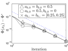
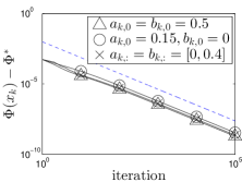
Fig. 1: (Left) $p=4$, (Right) $p=18$, $\Phi^{*}=0$. The dotted line is the slope of the predicted $O\left(k^{-\frac{p}{p-2}}\right)$ rate (i.e. ignoring constants). Note $a_{k,:}\triangleq[a_{k,0},a_{k,1}]$ and these are log-log plots.

7.2 SCAD and $\ell_{1}$ regularized Least-Squares

We solve Prob. (1) with $f(x)=\frac{1}{2}\|Ax-b\|_{2}^{2}$ and $g(x)=\sum_{i=1}^{n}r(x_{i})$ where $r$ is: 1) the SCAD regularizer defined as

$$r(x_{i})=\left\{\begin{array}[]{ll}\lambda|x_{i}|&\text{if }|x_{i}|\leq\lambda\\ -\frac{|x_{i}|^{2}-2a\lambda|x_{i}|+\lambda^{2}}{2(a-1)}&\text{if }\lambda<|x_{i}|\leq a\lambda\\ \frac{(a+1)\lambda^{2}}{2}&\text{if }|x_{i}|>a\lambda,\end{array}\right.$$

and 2) the absolute value $r(x_{i})=\lambda|x_{i}|$ leading to the $\ell_{1}$-norm. In both cases the proximal operator w.r.t. $r$ is easily computed. It was shown in [20, Sec. 5.2] and [19, Lemma 10] that both of these objective functions are KL functions with exponent $\theta=1/2$.

We choose $A\in\mathbb{R}^{500\times 1000}$ having i.i.d. $\mathcal{N}(0,10^{-4})$ entries, and $b=Ax_{0}$, where $x_{0}\in\mathbb{R}^{1000}$ has $50$ nonzero $\mathcal{N}(0,1)$-distributed entries. For SCAD we use $a=5$ and $\lambda=1$ and for the $\ell_{1}$ norm we use $\lambda=0.01$.

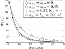
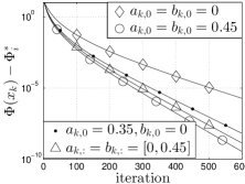
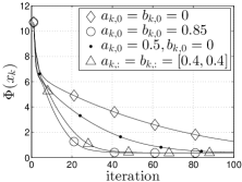
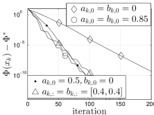
Fig. 2: (Top Left) Plot of $\Phi(x_{k})$ for SCAD least-squares. (Top Right) Plot of $\Phi(x_{k})-\Phi_{i}^{*}$ with a logarithmic $y$-axis for SCAD least-squares. As SCAD least-squares is a nonconvex problem, each of the four considered parameter choices may converge to a different objective function value $\Phi_{i}^{*}$ for $i=1,2,3,4$. (Bottom Left) Plot of $\Phi(x_{k})$ for $\ell_{1}$ least-squares. (Bottom Right) Plot of $\Phi(x_{k})-\Phi^{*}$ with a logarithmic $y$-axis for $\ell_{1}$ least-squares.

We consider four valid parameter choices. To isolate the effect of inertia, all choices used the same randomly chosen starting point and fixed stepsize, $\gamma_{k}=0.1/L$ for SCAD and $\gamma_{k}=1/L$ for $\ell_{1}$. The inertial parameters were chosen so that $\delta>0$ (defined in (4)) for SCAD and to satisfy [24, Thm. 1] for the $\ell_{1}$ problem. The two figures on the right corroborate Theorem 2 in that all considered parameter choices converge linearly to their limit, which was estimated by using the attained objective function value after $1000$ iterations. For the nonconvex SCAD this is a new result. For $\ell_{1}$-regularized least squares, inertial methods have been shown to achieve local linear convergence in [24, 31] under additional strict complementarity or restricted strong convexity assumptions. However, our analysis, which is based on the KL inequality, does not explicitly require these additional assumptions, as the objective function always has a KL exponent of $1/2$ [19, Lemma 10]. Furthermore our result proves global linear convergence, in that the KL inequality (2) holds for all $k$, implying $k_{0}=1$ in (5) and (8) holds for all $k$. In addition the two left figures show that the inertial choices appear to provide acceleration relative to the standard non-inertial choice which for SCAD is a new observation. This does not conflict with Theorem 2 which only shows that both non-inertial and inertial methods will converge linearly, however the convergence factor may be different. Estimating the factor is beyond the scope of this paper and we leave it for future work. Finally we mention that FISTA [32] and other Nesterov-accelerated methods [30] are not applicable to SCAD as it is nonconvex.

References

• [1] H. Attouch, J. Bolte, and B. F. Svaiter, “Convergence of descent methods for semi-algebraic and tame problems: proximal algorithms, forward–backward splitting, and regularized Gauss–Seidel methods,” Mathematical Programming, vol. 137, no. 1-2, pp. 91–129, 2013.
• [2] T. Blumensath and M. E. Davies, “Iterative thresholding for Sparse approximations,” Journal of Fourier Analysis and Applications, vol. 14, no. 5, pp. 629–654, Dec. 2008.
• [3] D. Lazzaro, “A nonconvex approach to low-rank matrix completion using convex optimization,” Numerical Linear Algebra with Applications, 2016.
• [4] M. Elad and M. Aharon, “Image denoising via sparse and redundant representations over learned dictionaries,” IEEE Transactions on Image processing, vol. 15, no. 12, pp. 3736–3745, 2006.
• [5] P. Chen and D. Suter, “Recovering the missing components in a large noisy low-rank matrix: Application to SFM,” IEEE transactions on pattern analysis and machine intelligence, vol. 26, no. 8, pp. 1051–1063, 2004.
• [6] H. H. Zhang, J. Ahn, X. Lin, and C. Park, “Gene selection using support vector machines with non-convex penalty,” Bioinformatics, vol. 22, no. 1, pp. 88–95, 2006.
• [7] E. J. Candes, Y. C. Eldar, T. Strohmer, and V. Voroninski, “Phase retrieval via matrix completion,” SIAM review, vol. 57, no. 2, pp. 225–251, 2015.
• [8] H. Ji, C. Liu, Z. Shen, and Y. Xu, “Robust video denoising using low rank matrix completion.,” in CVPR. Citeseer, 2010, pp. 1791–1798.
• [9] J. Fan and R. Li, “Variable selection via nonconcave penalized likelihood and its oracle properties,” Journal of the American statistical Association, vol. 96, no. 456, pp. 1348–1360, 2001.
• [10] P. L. Combettes and J.-C. Pesquet, “Proximal splitting methods in signal processing,” in Fixed-Point Algorithms for Inverse Problems in Science and Engineering, pp. 185–212. Springer, 2011.
• [11] B. T. Polyak, “Some methods of speeding up the convergence of iteration methods,” USSR Computational Mathematics and Mathematical Physics, vol. 4, no. 5, pp. 1–17, 1964.
• [12] R. I. Boţ, E. R. Csetnek, and S. C. László, “An inertial forward–backward algorithm for the minimization of the sum of two nonconvex functions,” EURO Journal on Computational Optimization, vol. 4, no. 1, pp. 3–25, 2016.
• [13] I. Sutskever, J. Martens, G. Dahl, and G. Hinton, “On the importance of initialization and momentum in deep learning,” in Proceedings of the 30th international conference on machine learning (ICML-13), 2013, pp. 1139–1147.
• [14] K. Kurdyka, “On gradients of functions definable in o-minimal structures,” in Annales de l’institut Fourier, 1998, vol. 48, pp. 769–783.
• [15] S. Lojasiewicz, “Une propriété topologique des sous-ensembles analytiques réels,” Les équations aux dérivées partielles, pp. 87–89, 1963.
• [16] H. Attouch, J. Bolte, P. Redont, and A. Soubeyran, “Proximal alternating minimization and projection methods for nonconvex problems: An approach based on the kurdyka-lojasiewicz inequality,” Mathematics of Operations Research, vol. 35, no. 2, pp. 438–457, 2010.
• [17] H. Attouch and J. Bolte, “On the convergence of the proximal algorithm for nonsmooth functions involving analytic features,” Mathematical Programming, vol. 116, no. 1-2, pp. 5–16, 2009.
• [18] P. Frankel, G. Garrigos, and J. Peypouquet, “Splitting methods with variable metric for KL functions,” arXiv preprint arXiv:1405.1357, 2014.
• [19] J. Bolte, T. P. Nguyen, J. Peypouquet, and B. Suter, “From error bounds to the complexity of first-order descent methods for convex functions,” arXiv preprint arXiv:1510.08234, 2015.
• [20] G. Li and T. K. Pong, “Calculus of the exponent of kurdyka-lojasiewicz inequality and its applications to linear convergence of first-order methods,” arXiv preprint arXiv:1602.02915, 2016.
• [21] P. Domingos, “A few useful things to know about machine learning,” Communications of the ACM, vol. 55, no. 10, pp. 78–87, 2012.
• [22] R. Ge, J. D. Lee, and T. Ma, “Matrix completion has no spurious local minimum,” arXiv preprint arXiv:1605.07272, 2016.
• [23] J. Liang, J. Fadili, and G. Peyré, “A multi-step inertial forward–backward splitting method for non-convex optimization,” arXiv preprint arXiv:1606.02118, 2016.
• [24] P. R. Johnstone and P. Moulin, “Local and global convergence of a general inertial proximal splitting scheme,” arXiv preprint arXiv:1602.02726, 2016.
• [25] P. Ochs, Y. Chen, T. Brox, and T. Pock, “iPiano: Inertial proximal algorithm for nonconvex optimization,” SIAM Journal on Imaging Sciences, vol. 7, no. 2, pp. 1388–1419, 2014.
• [26] S. Zavriev and F. Kostyuk, “Heavy-ball method in nonconvex optimization problems,” Computational Mathematics and Modeling, vol. 4, no. 4, pp. 336–341, 1993.
• [27] Y. Xu and W. Yin, “A block coordinate descent method for regularized multiconvex optimization with applications to nonnegative tensor factorization and completion,” SIAM Journal on imaging sciences, vol. 6, no. 3, pp. 1758–1789, 2013.
• [28] D. A. Lorenz and T. Pock, “An inertial forward-backward algorithm for monotone inclusions,” Journal of Mathematical Imaging and Vision, pp. 1–15, 2014.
• [29] J. Bolte, S. Sabach, and M. Teboulle, “Proximal alternating linearized minimization for nonconvex and nonsmooth problems,” Mathematical Programming, vol. 146, no. 1-2, pp. 459–494, 2014.
• [30] Y. Nesterov, Introductory lectures on convex optimization: a basic course, Springer, 2004.
• [31] J. Liang, J. Fadili, and G. Peyré, “Activity identification and local linear convergence of inertial forward-backward splitting,” arXiv preprint arXiv:1503.03703, 2015.
• [32] A. Beck and M. Teboulle, “Fast gradient-based algorithms for constrained total variation image denoising and deblurring problems,” Image Processing, IEEE Transactions on, vol. 18, no. 11, pp. 2419–2434, 2009.