h KA-TP-31-2016
2HDM Higgs-to-Higgs Decays
at Next-to-Leading Order

Abstract

The detailed investigation of the Higgs sector at present and future colliders necessitates from the theory side as precise predictions as possible, including higher order corrections. An important ingredient for the computation of higher order corrections is the renormalization of the model parameters and fields. In this paper we complete the renormalization of the 2-Higgs-Doublet Model (2HDM) Higgs sector launched in a previous contribution with the investigation of the renormalization of the mixing angles $\alpha$ and $\beta$. Here, we treat the renormalization of the mass parameter $m_{12}^{2}$ that softly breaks the $\mathbb{Z}_{2}$ symmetry of the 2HDM Higgs sector. We investigate the impact of two different renormalization schemes on the sample Higgs-to-Higgs decay $H\to hh$. This decay also allows us to analyze the renormalization of the mixing angles and to confirm the properties extracted before in other Higgs decays. In conclusion we find that a gauge-independent, process-independent and numerically stable renormalization of the 2HDM Higgs sector is given by the application of the tadpole-pinched scheme for the mixing angles $\alpha$ and $\beta$ and by the use of the $\overline{\mbox{MS}}$ scheme for $m_{12}^{2}$.

1 Introduction

The experimental data [1, 2, 3, 4] on the properties of the Higgs boson discovered in 2012 by the LHC experiments ATLAS [5] and CMS [6] are compatible with a Standard Model (SM)-like Higgs boson. Still they leave room for interpretations in models beyond the SM (BSM). Theoretical and experimental considerations lead to the conclusion that the SM cannot be the ultimate theory of nature. In view of no direct discovery of BSM manifestations in form of new particles so far, we are bound to study the Higgs sector in great detail in order to gain insights in possibly existing new physics (NP). Among the plethora of BSM extensions of the Higgs sector, 2-Higgs-Doublet Models (2HDM) [7, 8, 9] play an important role. They feature five physical Higgs bosons, two CP-even ones $h$ and $H$, a CP-odd scalar $A$ and two charged Higgs bosons $H^{\pm}$. The couplings of these Higgs bosons to SM particles are modified by two mixing angles, the angle $\alpha$ arising from the diagonalization of the CP-even Higgs mass matrix, and $\beta$ originating from the CP-odd and charged Higgs sectors. Together with singlet models, 2HDMs form the simplest SM extensions that are compatible with theoretical and experimental constraints [10, 11, 12, 13, 14]. Additionally, the Higgs sector of the Minimal Supersymmetric Extension of the SM (MSSM) [7, 15, 16, 17] represents a special case of the 2HDM type II. This allows to map insights gained in investigations of the 2HDM onto the MSSM and to compare effects that are possible in the less restricted 2HDM to the situation in the more restrained supersymmetric Higgs sector. The comparison of different models and, ultimately, the identification of the underlying theory requires experimental data at highest precision. Besides excellent experimental analysis techniques and the accumulation of a large amount of data at sufficiently high energy, this necessitates from the theory side precise predictions on observables and parameters, including higher order corrections. In a previous paper [18] we have provided an important basis for the computation of higher order (HO) corrections in the 2HDM by working out a manifestly gauge-independent renormalization of the two 2HDM mixing angles $\alpha$ and $\beta$, which is additionally process independent and numerically stable. The mixing angles play an important role for phenomenology, and we have investigated our renormalization scheme in the sample decays of the charged Higgs boson into a $W$ boson and a CP-even scalar, $H^{\pm}\to W^{\pm}h/H$, and of the heavy CP-even Higgs decay into a pair of $Z$ bosons, $H\to ZZ$.

In this paper we complete our renormalization of the 2HDM Higgs sector by computing the next-to-leading order (NLO) corrections to Higgs-to-Higgs decays. The investigation of these decays is of particular phenomenological interest. Not only they are a clear manifestation of an extended Higgs sector, they also give access to the trilinear Higgs self-couplings. The determination of these self-interactions constitutes a first important step towards the reconstruction of the Higgs potential [20, 21, 22], which is the final missing piece in the experimental verification of the Higgs mechanism. Higgs-to-Higgs decays can also be exploited for the discovery of non-SM Higgs bosons through cascade decays that are not accessible directly (see e.g. [23, 24, 25, 26, 27, 28, 29]). Interestingly, they can also be used to distinguish between different models [30]. It might even be that we see NP in Higgs pair production before anywhere else, i.e. in particular for Higgs couplings of the 125 GeV resonance which are SM-like [31].

Compared to the NLO computation of the Higgs decays presented in [18], the HO corrections to Higgs-to-Higgs decays require in addition the renormalization of the mass parameter $m_{12}^{2}$ of the Higgs potential. This parameter softly breaks the discrete $\mathbb{Z}_{2}$ symmetry, imposed to avoid tree-level flavour changing neutral currents (FCNC). We suggest different renormalization schemes for $m_{12}^{2}$ and investigate their numerical stability with respect to typical sizes of higher order corrections encountered in 2HDM Higgs-to-Higgs decays. The sample decay chosen in our analysis additionally allows us to study the numerical stability of the angular renormalization schemes proposed in [18] in a process which shows in the Higgs self-coupling a much more involved dependence on the mixing angles than the previously studied decays. In order to do so we identify the 2HDM parameter regions that lead to parametrically enhanced loop corrections due to non-decoupling effects. Subsequently, we analyze the loop corrections with respect to numerical stability in the decoupling regime where the heavy Higgs masses are due to a large mass scale independently of the Higgs self-couplings.

The paper is organized as follows. In section 2 we briefly introduce our model and set the notation. In the following section 3 we shortly review our renormalization conditions of [18], also needed here, and introduce the additionally required renormalization of $m_{12}^{2}$ entering the loop-corrected Higgs-to-Higgs decays. In section 4 we describe the calculation of the electroweak one-loop correction to the sample decay $H\to hh$. The numerical analysis is presented in section 5 in which we investigate our proposed renormalization procedures with respect to gauge independence, process independence and numerical stability. Our conclusions are given in section 6.

2 Description of the Model

Our work is performed within the framework of a general 2HDM with a global softly broken discrete $\mathbb{Z}_{2}$ symmetry. For the kinetic term of the two $SU(2)_{L}$ Higgs doublets $\Phi_{1}$ and $\Phi_{2}$ we introduce the covariant derivative

$$D_{\mu}=\partial_{\mu}+\frac{i}{2}g\sum_{a=1}^{3}\tau^{a}W_{\mu}^{a}+\frac{i}{2}g^{\prime}B_{\mu}\;,$$ (2.1)

where $\tau^{a}$ denote the Pauli matrices, $W_{\mu}^{a}$ and $B_{\mu}$ the $SU(2)_{L}$ and $U(1)_{Y}$ gauge bosons, respectively, and $g$ and $g^{\prime}$ the corresponding gauge couplings. The Higgs sector is described by the kinetic Lagrangian

$${\cal L}_{\text{kin}}=\sum_{i=1}^{2}(D_{\mu}\Phi_{i})^{\dagger}(D^{\mu}\Phi_{i})$$ (2.2)

and the scalar potential, which can be cast into the form

$$V = m_{11}^{2}|\Phi_{1}|^{2}+m_{22}^{2}|\Phi_{2}|^{2}-m_{12}^{2}(\Phi_{1}^{\dagger}\Phi_{2}+h.c.)+\frac{\lambda_{1}}{2}(\Phi_{1}^{\dagger}\Phi_{1})^{2}+\frac{\lambda_{2}}{2}(\Phi_{2}^{\dagger}\Phi_{2})^{2}$$ (2.3)

$$+\lambda_{3}(\Phi_{1}^{\dagger}\Phi_{1})(\Phi_{2}^{\dagger}\Phi_{2})+\lambda_{4}(\Phi_{1}^{\dagger}\Phi_{2})(\Phi_{2}^{\dagger}\Phi_{1})+\frac{\lambda_{5}}{2}[(\Phi_{1}^{\dagger}\Phi_{2})^{2}+h.c.]\;.$$

The absence of FCNCs at tree level is ensured by imposing the discrete $\mathbb{Z}_{2}$ symmetry under which the doublets transform as $\Phi_{1}\to-\Phi_{1}$ and $\Phi_{2}\to\Phi_{2}$. We assume CP conservation so that the 2HDM potential depends on eight real parameters, three mass parameters, $m_{11}$, $m_{22}$ and $m_{12}$, and five coupling parameters $\lambda_{1}$-$\lambda_{5}$. As can be inferred from the potential, a non-zero value of $m_{12}^{2}$ softly breaks the discrete $\mathbb{Z}_{2}$ symmetry. The two doublet fields $\Phi_{1}$ and $\Phi_{2}$ can be expressed in terms of charged complex fields $\phi_{i}^{+}$ and real neutral CP-even and CP-odd fields $\rho_{i}$ and $\eta_{i}$ ($i=1,2$), respectively. By expanding the two Higgs doublets about their vacuum expectation values (VEVs), developed after electroweak symmetry breaking (EWSB), which are real in the CP-conserving case,

$$\Phi_{1}=\left(\begin{array}[]{c}\phi_{1}^{+}\\ \frac{\rho_{1}+i\eta_{1}+v_{1}}{\sqrt{2}}\end{array}\right)\qquad\mbox{and}\qquad\Phi_{2}=\left(\begin{array}[]{c}\phi_{2}^{+}\\ \frac{\rho_{2}+i\eta_{2}+v_{2}}{\sqrt{2}}\end{array}\right)\;,$$ (2.8)

the mass matrices can be derived from the terms bilinear in the Higgs fields in the Higgs potential. Under the assumption of charge and CP conservation they decompose into $2\times 2$ matrices ${\cal M}_{S}$, ${\cal M}_{P}$ and ${\cal M}_{C}$ for the neutral CP-even, neutral CP-odd and charged Higgs sectors. For the two Higgs doublets $\Phi_{i}$ to take their minimum at $\langle\Phi_{i}\rangle\equiv v_{i}$ the minimum conditions

$$\left.\frac{\partial V}{\partial\Phi_{1}}\right|_{\langle\Phi_{i}\rangle}=\left.\frac{\partial V}{\partial\Phi_{2}}\right|_{\langle\Phi_{i}\rangle}=0\;,$$ (2.9)

have to be fulfilled. This is equivalent to the requirement of the two terms linear in $\rho_{1}$ and $\rho_{2}$ to vanish, i.e.

$$\frac{T_{1}}{v_{1}} = m_{11}^{2}-m_{12}^{2}\frac{v_{2}}{v_{1}}+\frac{\lambda_{1}v_{1}^{2}}{2}+\frac{\lambda_{345}v_{2}^{2}}{2}$$ (2.10)

$$\frac{T_{2}}{v_{2}} = m_{22}^{2}-m_{12}^{2}\frac{v_{1}}{v_{2}}+\frac{\lambda_{2}v_{2}^{2}}{2}+\frac{\lambda_{345}v_{1}^{2}}{2}\;.$$ (2.11)

The tadpole conditions can be exploited to replace $m_{11}^{2}$ and $m_{22}^{2}$ by the tadpole parameters $T_{1}$ and $T_{2}$. This yields the following explicit form of the mass matrices

$${\cal M}_{S} = \left(\begin{array}[]{cc}m_{12}^{2}\frac{v_{2}}{v_{1}}+\lambda_{1}v_{1}^{2}&-m_{12}^{2}+\lambda_{345}v_{1}v_{2}\\ -m_{12}^{2}+\lambda_{345}v_{1}v_{2}&m_{12}^{2}\frac{v_{1}}{v_{2}}+\lambda_{2}v_{2}^{2}\end{array}\right)+\left(\begin{array}[]{cc}\frac{T_{1}}{v_{1}}&0\\ 0&\frac{T_{2}}{v_{2}}\end{array}\right)$$ (2.16)

$${\cal M}_{P} = \left(\frac{m_{12}^{2}}{v_{1}v_{2}}-\lambda_{5}\right)\left(\begin{array}[]{cc}v_{2}^{2}&-v_{1}v_{2}\\ -v_{1}v_{2}&v_{1}^{2}\end{array}\right)+\left(\begin{array}[]{cc}\frac{T_{1}}{v_{1}}&0\\ 0&\frac{T_{2}}{v_{2}}\end{array}\right)$$ (2.21)

$${\cal M}_{C} = \left(\frac{m_{12}^{2}}{v_{1}v_{2}}-\frac{\lambda_{4}+\lambda_{5}}{2}\right)\left(\begin{array}[]{cc}v_{2}^{2}&-v_{1}v_{2}\\ -v_{1}v_{2}&v_{1}^{2}\end{array}\right)+\left(\begin{array}[]{cc}\frac{T_{1}}{v_{1}}&0\\ 0&\frac{T_{2}}{v_{2}}\end{array}\right)\;,$$ (2.26)

where we introduced the abbreviation

$$\lambda_{345}\equiv\lambda_{3}+\lambda_{4}+\lambda_{5}\;.$$ (2.27)

In Eqs. (2.16)-(2.26) we explicitly kept the tadpole parameters $T_{1}$ and $T_{2}$, which vanish at tree level, in order to ensure the correct treatment of the minimum conditions beyond leading order (LO). The diagonal mass matrices of the physical states can be obtained by performing the following orthogonal transformations

$$\left(\begin{array}[]{c}\rho_{1}\\ \rho_{2}\end{array}\right) = R(\alpha)\left(\begin{array}[]{c}H\\ h\end{array}\right)\;,$$ (2.32)

$$\left(\begin{array}[]{c}\eta_{1}\\ \eta_{2}\end{array}\right) = R(\beta)\left(\begin{array}[]{c}G^{0}\\ A\end{array}\right)\;,$$ (2.37)

$$\left(\begin{array}[]{c}\phi_{1}^{\pm}\\ \phi^{\pm}_{2}\end{array}\right) = R(\beta)\left(\begin{array}[]{c}G^{\pm}\\ H^{\pm}\end{array}\right)\;,$$ (2.42)

which lead to the physical Higgs states, a neutral light CP-even, $h$, a neutral heavy CP-even, $H$, a neutral CP-odd, $A$, and two charged Higgs bosons, $H^{\pm}$. The also obtained massless pseudo-Nambu-Goldstone bosons $G^{\pm}$ and $G^{0}$ form the longitudinal components of the massive gauge bosons, the charged $W^{\pm}$ and the $Z$ boson, respectively. In terms of the mixing angles $\vartheta=\alpha$ and $\beta$, respectively, the rotation matrices read

$$R(\vartheta)=\left(\begin{array}[]{cc}\cos\vartheta&-\sin\vartheta\\ \sin\vartheta&\cos\vartheta\end{array}\right)\;.$$ (2.45)

The mixing angle $\beta$ can be expressed through the ratio of the two VEVs,

$$\tan\beta=\frac{v_{2}}{v_{1}}\;,$$ (2.46)

with the phenomenological constraint $v_{1}^{2}+v_{2}^{2}=v^{2}\approx(246\mbox{ GeV})^{2}$. The mixing angle $\alpha$ on the other hand can be parametrized in terms of the entries $({\cal M}_{S})_{ij}$ ($i,j=1,2$) of the CP-even scalar mass matrix as

$$\tan 2\alpha=\frac{2({\cal M}_{S})_{12}}{({\cal M}_{S})_{11}-({\cal M}_{S})_{22}}\;.$$ (2.47)

Introducing the abbreviation

$$M^{2}\equiv\frac{m_{12}^{2}}{s_{\beta}c_{\beta}}$$ (2.48)

and the short-hand notation $s_{x}\equiv\sin x$ etc., we have [32]

$$\tan 2\alpha=\frac{s_{2\beta}(M^{2}-\lambda_{345}v^{2})}{c_{\beta}^{2}(M^{2}-\lambda_{1}v^{2})-s_{\beta}^{2}(M^{2}-\lambda_{2}v^{2})}\;.$$ (2.49)

After diagonalization the physical masses are given by

$$m_{h,H}^{2} = \frac{1}{2}\left[({\cal M}_{S})_{11}+({\cal M}_{S})_{22}\mp\sqrt{\left(({\cal M}_{S})_{11}-({\cal M}_{S})_{22}\right)^{2}+4(({\cal M}_{S})_{12})^{2}}\right]$$ (2.50)

$$m_{A}^{2} = M^{2}-\lambda_{5}v^{2}$$ (2.51)

$$m_{H^{\pm}}^{2} = M^{2}-\frac{\lambda_{4}+\lambda_{5}}{2}v^{2}\;.$$ (2.52)

Note, in particular, that the masses of the heavier Higgs bosons, $\phi_{\text{heavy}}=H,A$ and $H^{\pm}$, take the form [32]

$$m_{\phi_{\text{heavy}}}^{2}=c_{\phi_{\text{heavy}}}^{2}M^{2}+f(\lambda_{i})\,v^{2}+{\cal O}(v^{4}/M^{2})\;,$$ (2.53)

where $f(\lambda_{i})$ denotes a linear combination of $\lambda_{1}-\lambda_{5}$. The coefficient $c_{\phi_{\text{heavy}}}$ is given by

$$c_{\phi_{\text{heavy}}}=\left\{\begin{array}[]{ll}1&\mbox{for }\;\phi_{\text{heavy}}=A,H^{\pm}\\ s_{\beta-\alpha}&\mbox{for }\;\phi_{{\text{heavy}}}=H\end{array}\right.\;.$$ (2.56)

There are two interesting limits that will play an important role in the relative size of the NLO corrections. For $c_{\phi_{\text{heavy}}}^{2}M^{2}\gg f(\lambda_{i})\,v^{2}$ we are in the decoupling limit. In the opposite case, if $M^{2}\raisebox{-3.69899pt}{~{}\shortstack{$<$ \\ [-0.07cm] $\sim$}}~{}f(\lambda_{i})\,v^{2}$ and the Higgs boson masses are large, we are in the strong coupling regime, as we then need the coupling strengths to be significant. Both regimes will be investigated in detail in the numerical analysis.

For the parametrization of the Higgs potential $V$ there are various possibilities to choose the set of independent parameters. Our guideline is given by the wish to relate the parameters to as many physical quantities as possible. Thus we express the VEV $v$ in terms of the physical gauge boson masses $M_{W}$ and $M_{Z}$ and the electric charge $e$, and replace $m_{11}^{2}$ and $m_{22}^{2}$ by the tadpole parameters $T_{1}$ and $T_{2}$. Later, we will also choose the renormalization through Higgs decays. For this we need the fermion masses $m_{f}$. Our set of independent parameters is then given by the Higgs boson masses, the tadpole parameters, the two mixing angles, the soft breaking parameter, the massive gauge boson masses, the electric charge and the fermion masses:

$$\mbox{\text@underline{Input parameters:}}\quad m_{h},\;m_{H},\;m_{A},\;m_{H^{\pm}},\;T_{1},\;T_{2},\;\alpha,\;\tan\beta,\;m_{12}^{2},\;M_{W}^{2},\;M_{Z}^{2},\;e,\;m_{f}\;.$$ (2.57)

3 Renormalization

The one-loop computation of our sample Higgs-to-Higgs decay process

$$H\to hh\;,$$ (3.1)

encounters ultraviolet (UV) divergences. These are cancelled by the renormalization of the parameters and wave functions involved in the process. In particular, the process requires the renormalization of the gauge sector and the Higgs sector of the 2HDM. In [18] we proposed several renormalization schemes for the mixing angles $\alpha$ and $\beta$, among these also the process-dependent renormalization through the decays $H\to\tau\tau$ and $A\to\tau\tau$. These processes additionally require the renormalization of the fermion sector. Here, we first briefly repeat the basic features of our chosen renormalization conditions that have been described in [18], with emphasis on the renormalization of the mixing angles. For further details, we refer the reader to [18]. We then present the renormalization of the soft breaking parameter $m_{12}^{2}$, which is required in the loop-corrected Higgs-to-Higgs decays.

For the renormalization, the bare parameters $p_{0}$ involved in the process have to be replaced by the renormalized ones, $p$, and the corresponding counterterms $\delta p$,

$$p_{0}=p+\delta p\;.$$ (3.2)

Additionally the fields $\Psi$ are renormalized by their field renormalization constants $\delta Z_{\Psi}$ as

$$\Psi_{0}=\sqrt{Z_{\Psi}}\Psi\;,$$ (3.3)

where $\Psi$ generically stands for scalar, vector and fermion fields. Note, that $Z_{\Psi}$ is a matrix in case of mixing fields. All Higgs bosons, gauge bosons and fermions are renormalized on-shell (OS). The electric charge, which enters the weak gauge couplings, is defined to be the full electron-positron photon coupling for OS particles in the Thomson limit. Note, that we will use the fine-structure constant at the $Z$ boson mass, $\alpha(M_{Z}^{2})$, as input in order to avoid large logarithms due to light fermions $f\neq t$. The renormalization conditions for the tadpoles are chosen such that the correct vacuum is reproduced at one-loop order which implies

$$\delta T_{i}=T_{i}\;,\qquad i=1,2\;,$$ (3.4)

where the $T_{i}$ stand for the contributions from the genuine Higgs boson tadpole graphs in the gauge basis.

3.1 Renormalization of the Mixing Angles

In [18] we discussed in great detail the renormalization of the mixing angles $\alpha$ and $\beta$. In particular, schemes used in the literature before were shown to lead to gauge-dependent decay amplitudes. This is based on the fact that the standard treatment of the tadpoles, the standard tadpole scheme, leads to gauge-dependent counterterms for the masses and mixing angles. In particular, a gauge-independent decay amplitude can then only be obtained through a physical, e.g. a process-dependent, definition of the angular counterterms. In the standard tadpole scheme the correct vacuum at higher orders is given by the VEV that is derived from the gauge-dependent loop-corrected Higgs potential, and is therefore also gauge dependent. Consequently, all bare quantities and counterterms given in terms of the VEV become gauge dependent as well. In the alternative tadpole scheme [33], the bare quantities are not gauge dependent, as they are expressed in terms of the tree-level VEV, which is gauge independent. The correct minimum at higher orders is reproduced by shifting the VEV. The shift affects the counterterms but not the bare quantities. With the exception of the wave function renormalization constants, the counterterms are gauge independent in the alternative tadpole scheme. In practice the change from the standard to the alternative tadpole scheme, also referred to as standard and tadpole scheme, respectively, requires the following modifications:

• Self-energies: The self-energies in the wave function renormalization constants and counterterms have to be changed to contain additional tadpole contributions: $\Sigma(p^{2})\to\Sigma^{\text{tad}}(p^{2})$.

• Tadpole counterterms: In turn, the tadpole counterterms do not appear any more in the scalar sector: $\delta T_{\phi_{i}\phi_{j}}\to 0$.

• Vertex corrections: In the virtual corrections additional tadpole contributions have be taken into account if the extension of the corresponding coupling by an external CP-even Higgs boson $h,H$, which carries the tadpole, exists.

For all details, we refer the reader to Appendix A of [18].

In [18] the tadpole-pinched scheme was introduced as a manifestly gauge-independent renormalization scheme for the angular counterterms. It relies on the use of the alternative tadpole scheme together with the modified Higgs self-energies defined by means of the pinch technique [34, 35, 36, 37, 38, 39, 40]. The angular counterterms are obtained in terms of the pinched self-energies $\overline{\Sigma}(p^{2})$, where $p^{2}$ denotes the four-momenta squared at which they are evaluated. Note that they have to be evaluated in the tadpole scheme and can be related to the tadpole self-energies in the Feynman gauge through

$$\overline{\Sigma}(p^{2})=\left.\Sigma^{\text{tad}}(p^{2})\right|_{\xi=1}+\Sigma^{\text{add}}(p^{2})\;.$$ (3.5)

Here $\xi$ represents the gauge fixing parameters $\xi_{Z},$ $\xi_{W}$ and $\xi_{\gamma}$ of the $R_{\xi}$ gauge. For the renormalization of the mixing angle $\beta$ the pseudoscalar or the charged sector can be used, leading to different counterterm definitions. We will use two different definitions, specified below. We will furthermore apply two different tadpole-pinched schemes which differ by their choice of the renormalization scale:

On-shell tadpole-pinched scheme: The renormalization scale is chosen to be the on-shell scale in the appearing self-energies. Applying [56], the angular counterterms are given by

$$\delta\alpha = \frac{\mbox{Re}\left(\left[\Sigma_{Hh}^{\text{tad}}(m_{H}^{2})+\Sigma^{\text{tad}}_{Hh}(m_{h}^{2})\right]_{\xi=1}+\Sigma^{\text{add}}_{Hh}(m_{H}^{2})+\Sigma^{\text{add}}_{Hh}(m_{h}^{2})\right)}{2(m_{H}^{2}-m_{h}^{2})}$$ (3.6)

$$\delta\beta^{(1)} = -\frac{\mbox{Re}\left(\left[\Sigma_{G^{\pm}H^{\pm}}^{\text{tad}}(0)+\Sigma^{\text{tad}}_{G^{\pm}H^{\pm}}(m_{H^{\pm}}^{2})\right]_{\xi=1}+\Sigma^{\text{add}}_{G^{\pm}H^{\pm}}(0)+\Sigma^{\text{add}}_{G^{\pm}H^{\pm}}(m_{H^{\pm}}^{2})\right)}{2m_{H^{\pm}}^{2}}$$ (3.7)

$$\delta\beta^{(2)} = -\frac{\mbox{Re}\left(\left[\Sigma_{G^{0}A}^{\text{tad}}(0)+\Sigma^{\text{tad}}_{G^{0}A}(m_{A}^{2})\right]_{\xi=1}+\Sigma^{\text{add}}_{G^{0}A}(0)+\Sigma^{\text{add}}_{G^{0}A}(m_{A}^{2})\right)}{2m_{A}^{2}}\;.$$ (3.8)

The additional contributions read (see also [56] for the CP-even case in the MSSM),

$$\Sigma^{\text{add}}_{Hh}(p^{2}) = \frac{g^{2}s_{\beta-\alpha}c_{\beta-\alpha}}{32\pi^{2}c_{W}^{2}}\left(p^{2}-\frac{m_{H}^{2}+m_{h}^{2}}{2}\right)\Big{\{}B_{0}(p^{2};m_{Z}^{2},m_{A}^{2})-B_{0}(p^{2};m_{Z}^{2},m_{Z}^{2})$$ (3.9)

$$+2c_{W}^{2}\left[B_{0}(p^{2};m_{W}^{2},m_{H^{\pm}}^{2})-B_{0}(p^{2};m_{W}^{2},m_{W}^{2})\right]\Big{\}}$$

$$\Sigma^{\text{add}}_{G^{0}A}(p^{2}) = \frac{g^{2}s_{\beta-\alpha}c_{\beta-\alpha}}{32\pi^{2}c_{W}^{2}}\left(p^{2}-\frac{m_{A}^{2}}{2}\right)\left[B_{0}(p^{2};m_{Z}^{2},m_{H}^{2})-B_{0}(p^{2};m_{Z}^{2},m_{h}^{2})\right]$$ (3.10)

$$\Sigma^{\text{add}}_{G^{\pm}H^{\pm}}(p^{2}) = \frac{g^{2}s_{\beta-\alpha}c_{\beta-\alpha}}{16\pi^{2}}\left(p^{2}-\frac{m_{H^{\pm}}^{2}}{2}\right)\left[B_{0}(p^{2};m_{W}^{2},m_{H}^{2})-B_{0}(p^{2};m_{W}^{2},m_{h}^{2})\right]\;,$$ (3.11)

where $B_{0}$ is the scalar two-point function [57, 58] and $c_{W}$ refers to the cosine of the Weinberg angle $\theta_{W}$.

$p_{\star}$ tadpole-pinched scheme: In this scheme the self-energies are evaluated at the average of the particle momenta squared [56],

$$p_{\star}^{2}=\frac{m_{\phi_{1}}^{2}+m_{\phi_{2}}^{2}}{2}\;,$$ (3.12)

with $(\phi_{1},\phi_{2})=(H,h)$, $(G^{\pm},H^{\pm})$ and $(G^{0},A)$, respectively. The additional contributions then obviously vanish and the angular counterterms simplify to

$$\delta\alpha = \frac{\mbox{Re}\left[\overline{\Sigma}_{Hh}\left(\frac{m_{h}^{2}+m_{H}^{2}}{2}\right)\right]}{m_{H}^{2}-m_{h}^{2}}$$ (3.13)

$$\delta\beta^{(1)} = -\frac{\mbox{Re}\left[\overline{\Sigma}_{G^{\pm}H^{\pm}}\left(\frac{m_{H^{\pm}}^{2}}{2}\right)\right]}{m_{H^{\pm}}^{2}}$$ (3.14)

$$\delta\beta^{(2)} = -\frac{\mbox{Re}\left[\overline{\Sigma}_{G^{0}A}\left(\frac{m_{A}^{2}}{2}\right)\right]}{m_{A}^{2}}\;.$$ (3.15)

Process-dependent renormalization: We also apply a process-dependent renormalization of the mixing angles. The angular counterterm $\delta\beta$ is obtained from the requirement that the loop-corrected Higgs decay $A\to\tau\tau$ including only the weak corrections is equal to the LO width,

$$\Gamma^{\text{LO}}(A\to\tau\tau)\stackrel{{\scriptstyle!}}{{=}}\Gamma^{\text{NLO}}_{\text{weak}}(A\to\tau\tau)\;.$$ (3.16)

The counterterm $\delta\alpha$ is obtained by applying the same condition, but on the $H\to\tau\tau$ decay,

$$\Gamma^{\text{LO}}(H\to\tau\tau)\stackrel{{\scriptstyle!}}{{=}}\Gamma^{\text{NLO}}_{\text{weak}}(H\to\tau\tau)\;.$$ (3.17)

The process-dependent renormalization leads to gauge-dependent angular counterterms if the standard tadpole scheme is applied. The angular counterterms are manifestly gauge independent, on the other hand, in case the alternative tadpole scheme is used.

3.2 Renormalization of $m_{12}^{2}$

For the renormalization of the soft $\mathbb{Z}_{2}$ breaking parameter $m_{12}^{2}$ the bare parameter is replaced by the renormalized one and its counterterm,

$$(m_{12}^{2})_{0}=m_{12}^{2}+\delta m_{12}^{2}\;.$$ (3.18)

We will apply two different renormalization schemes.

Modified Minimal Subtraction Scheme: In the modified minimal subtraction ($\overline{\mbox{MS}}$) scheme the counterterm $\delta m_{12}^{2}$ is chosen such that it cancels all residual terms of the amplitude, which are proportional to

$$\Delta=\frac{1}{\epsilon}-\gamma_{E}+\ln(4\pi)\;,$$ (3.19)

where $\gamma_{E}$ denotes the Euler-Mascheroni constant. These terms obviously contain the remaining UV divergences given as poles in $\epsilon$ plus additional finite constants that appear universally in all loop integrals [61]. The renormalization of $\delta m_{12}^{2}$ in this scheme is hence given by

$$\delta m_{12}^{2}=\delta m_{12}^{2}(\Delta)|_{\overline{\text{MS}}}\;,$$ (3.20)

where the right-hand side of the equation symbolically denotes all terms proportional to $\Delta$ that are necessary to cancel the $\Delta$ dependence of the remainder of the amplitude.

Process-dependent renormalization: A more physical definition of the counterterm is provided by the renormalization through a physical process. As $m_{12}^{2}$ only appears in the couplings between Higgs bosons, the simplest processes that can be chosen to fix the counterterm are given by the on-shell decays

$$H \to hh$$ (3.21)

$$H \to H^{+}H^{-}$$ (3.22)

$$h \to AA$$ (3.23)

$$H \to AA\;.$$ (3.24)

As the scalar $h$ is identified with the 125 GeV Higgs boson the decay $h\to H^{+}H^{-}$ is kinematically not possible, since we restrict the charged Higgs mass to $m_{H^{\pm}}>m_{h}$, see e.g. [62] for a type II 2HDM. We will compute the loop corrections to the decay $H\to hh$ in order to study the impact of the various renormalization schemes, so that this process cannot be used for the determination of $\delta m_{12}^{2}$. With $H^{\pm}$ masses above 480 GeV in the type II 2HDM [62], which we will choose for the numerical analysis, the decay $H\to H^{+}H^{-}$ would require very heavy $H$ bosons, so that we do not consider this process either. The OS process $h\to AA$ is kinematically very restricted as it requires pseudoscalars $A$ with masses below 125 GeV/2 that additionally have escaped detection at collider experiments so far. Although such scenarios are possible in principle, they are very rare, and the measurement of the decay is challenging. This leaves us with the process $H\to AA$ as the least restrictive one to fix the counterterm of $\delta m_{12}^{2}$.

Note, that $\delta m_{12}^{2}$ in both schemes is gauge independent irrespective of the chosen tadpole scheme. Being a parameter of the original 2HDM Higgs potential before EWSB, it is not related to the VEV and hence cannot encounter any gauge dependences arising from the treatment of the VEV at higher orders.

4 Decay Widths at Electroweak One-Loop Order

We will present here the details for the computation of the electroweak one-loop corrections to the Higgs-to-Higgs decay widths

$$H \to hh\qquad\mbox{ and}$$ (4.25)

$$H \to AA\;.$$ (4.26)

The first process will be used to study numerically the impact of the various renormalization schemes that we propose on the NLO corrections. The second process serves for a process-dependent definition of the counterterm $\delta m_{12}^{2}$.

4.1 Electroweak One-Loop Corrections to $H\to hh$

The heavy Higgs decay into a pair of SM-like Higgs bosons,

$$H\to hh\;,$$ (4.27)

depends through the trilinear Higgs self-coupling

$$\lambda_{Hhh}\equiv g\cdot g_{Hhh}=g\frac{-c_{\beta-\alpha}}{2M_{W}s_{2\beta}}\left(s_{2\alpha}(2m_{h}^{2}+m_{H}^{2})-\frac{m_{12}^{2}}{s_{\beta}c_{\beta}}(3s_{2\alpha}-s_{2\beta})\right)$$ (4.28)

not only on the mixing angles $\alpha$ and $\beta$ but also on $m_{12}^{2}$. The LO decay width is given by

$$\Gamma^{\text{LO}}(H\to hh)=\frac{G_{F}M_{W}^{2}m_{H}g_{Hhh}^{2}}{4\sqrt{2}\pi}\sqrt{1-\frac{4m_{h}^{2}}{m_{H}^{2}}}\;,$$ (4.29)

where $G_{F}$ denotes the Fermi constant. The NLO decay width can be written as the sum of the LO width and the one-loop corrected decay width $\Gamma^{(1)}$,

$$\Gamma^{\text{NLO}}=\Gamma^{\text{LO}}+\Gamma^{(1)}\;.$$ (4.30)

The one-loop correction $\Gamma^{(1)}$ is obtained from the interference of the LO decay amplitude with the one at NLO. The contributions to the NLO decay amplitude are given by the virtual corrections and the counterterm diagrams. The virtual corrections consist of the pure vertex corrections, shown in Fig. 1, and the corrections to the external legs. The vertex corrections comprise the one-particle irreducible (1PI) diagrams given by the triangle diagrams with fermions, scalars, ghosts and gauge bosons in the loops and the diagrams involving four-particle vertices.

Figure 1: Generic diagrams contributing to the vertex corrections in $H\to hh$ with fermions $F$, scalar bosons $S$, ghosts $U$ and gauge bosons $V$ in the loops.

The external leg corrections consist of off-diagonal and diagonal field mixing contributions $hH,Hh,HH$ and $hh$, which all vanish due to the OS renormalization conditions of the external fields. The counterterm diagrams are shown in Fig. 2. They are given by all possible counterterm insertions on the external legs and the genuine vertex counterterm.

Figure 2: Counterterm diagrams contributing to the NLO decay $H\to hh$.

For the correct derivation of the symmetry factors associated with the various counterterm contributions we start from the bare Lagrangian describing the involved trilinear Higgs self-interactions. In terms of the coupling factors

$$g_{hhh} = \frac{3}{2M_{W}s_{2\beta}}\left(\frac{2m_{12}^{2}}{s_{\beta}c_{\beta}}c_{\alpha+\beta}c_{\beta-\alpha}^{2}-m_{h}^{2}(2c_{\alpha+\beta}+s_{2\alpha}s_{\beta-\alpha})\right)$$ (4.31)

$$g_{HHh} = \frac{s_{\beta-\alpha}}{2M_{W}s_{2\beta}}\left(-\frac{m_{12}^{2}}{s_{\beta}c_{\beta}}(3s_{2\alpha}+s_{2\beta})+s_{2\alpha}(m_{h}^{2}+2m_{H}^{2})\right)$$ (4.32)

and $g_{Hhh}$ defined in Eq. (4.28) it reads

$${\cal L}_{\text{int}}^{Hhh} = g\left[\frac{-g_{hhh}}{3!}h_{0}h_{0}h_{0}-\frac{g_{Hhh}}{2!}H_{0}h_{0}h_{0}-\frac{g_{HHh}}{2!}H_{0}H_{0}h_{0}\right]\;,$$ (4.33)

where $h_{0}$ and $H_{0}$ denote the bare fields. At NLO we obtain in terms of the renormalized fields $h$ and $H$,

$${\cal L}_{\text{int}}^{Hhh} \stackrel{{\scriptstyle\text{NLO}}}{{\approx}} g\left[\frac{-g_{hhh}}{3!}\frac{3\delta Z_{hH}}{2}-\frac{g_{Hhh}}{2!}\left(\delta Z_{hh}+\frac{\delta Z_{HH}}{2}\right)-\frac{g_{HHh}}{2!}\delta Z_{Hh}\right]Hhh\;,$$ (4.34)

where the $\delta Z$’s denote the wave function renormalization constants. The Feynman rule $\lambda_{\text{CT,WR}}^{Hhh}$ for this counterterm contribution from the wave function renormalization is derived by applying the functional derivatives with respect to the external renormalized fields,

$$\lambda_{\text{CT,WR}}^{Hhh} = i\frac{\delta}{i\delta H}\frac{\delta}{i\delta h}\frac{\delta}{i\delta h}{\cal L}_{\text{int}}^{Hhh}\;.$$ (4.35)

Adding the genuine vertex counterterm $\delta(g\cdot g_{Hhh})$ we have for the counterterm amplitude

$${\cal M}_{Hhh}^{\text{CT}}=g\left[g_{hhh}\frac{\delta Z_{hH}}{2}+g_{Hhh}\left(\delta Z_{hh}+\frac{\delta Z_{HH}}{2}\right)+g_{HHh}\delta Z_{Hh}+\frac{1}{g}\delta(g\cdot g_{Hhh})\right]\;.$$ (4.36)

The genuine vertex counterterm at NLO is given by

$$\delta(g\cdot g_{Hhh}) = g\Big{\{}g_{Hhh}\left(\frac{\delta g}{g}-\frac{\delta M_{W}}{M_{W}}\right)$$ (4.37)

$$\;+\left(\frac{-c_{\beta-\alpha}}{M_{W}s_{2\beta}}\right)\left[\frac{s_{2\alpha}}{2}(2\delta m_{h}^{2}+\delta m_{H}^{2})-\left(\frac{3s_{2\alpha}-s_{2\beta}}{s_{2\beta}}\right)\delta m_{12}^{2}\right]$$

$$\;+\left[g_{Hhh}\left(-t_{\beta-\alpha}-\frac{2}{t_{2\beta}}\right)-\frac{m_{12}^{2}}{M_{W}}\left(\frac{c_{\beta-\alpha}}{s_{2\beta}^{2}}\right)\frac{6s_{2\alpha}}{t_{2\beta}}\right]\delta\beta$$

$$\;+\left[g_{Hhh}t_{\beta-\alpha}-\frac{2m_{h}^{2}+m_{H}^{2}-3m_{12}^{2}/(s_{\beta}c_{\beta})}{M_{W}}\frac{c_{\beta-\alpha}c_{2\alpha}}{s_{2\beta}}\right]\delta\alpha\Big{\}}\;.$$

The NLO corrections factorize from the LO amplitude so that the one-loop corrected decay width can be cast into the form

$$\Gamma^{\text{NLO}}(H\to hh)=\Gamma^{\text{LO}}\left[1+\Delta^{\text{virt}}_{Hhh}+\Delta^{\text{ct}}_{Hhh}\right]\;,$$ (4.38)

with $\Delta^{\text{ct}}_{Hhh}$ given by

$$\Delta^{\text{ct}}=\frac{2{\cal M}_{Hhh}^{\text{CT}}}{g\cdot g_{Hhh}}\;.$$ (4.39)

The expression $\Delta^{\text{virt}}_{Hhh}$ is quite lengthy so that we do not display it explicitly here.

Figure 3: Additional vertex diagrams in the alternative tadpole scheme contributing to the decay $H\to hh$.

In case the alternative tadpole scheme is applied, additional diagrams have to be included in the virtual corrections. They are depicted in Fig. 3 and involve quartic Higgs self-couplings where the additionally attached Higgs to the original trilinear vertex is connected to a tadpole diagram. The inclusion of these additional diagrams in combination with the change of the mass, angular and wave function counterterms in the alternative tadpole scheme leaves the overall NLO decay width invariant, provided the angular counterterms are defined in a process dependent scheme.

4.2 Electroweak One-Loop Corrections to $H\to AA$

We use the decay of the heavy scalar $H$ into a pair of pseudoscalars $A$,

$$H\to AA\;,$$ (4.40)

for a process-dependent renormalization of $m_{12}^{2}$. The leading order decay width depends through the trilinear coupling

$$\lambda_{HAA}\equiv g\cdot g_{HAA}=-\frac{g}{2M_{W}}\left[c_{\beta-\alpha}(2m_{A}^{2}-m_{H}^{2})+\frac{s_{\alpha+\beta}}{s_{2\beta}}\left(2m_{H}^{2}-\frac{2m_{12}^{2}}{s_{\beta}c_{\beta}}\right)\right]$$ (4.41)

besides on the mixing angles $\alpha$ and $\beta$ in particular on $m_{12}^{2}$. The LO decay width is given by

$$\Gamma^{\text{LO}}(H\to AA)=\frac{G_{F}M_{W}^{2}m_{H}g_{HAA}^{2}}{4\sqrt{2}\pi}\sqrt{1-\frac{4m_{A}^{2}}{m_{H}^{2}}}\;.$$ (4.42)

The electroweak (EW) one-loop corrections consist of the virtual corrections and the counterterm contributions which guarantee the UV-finiteness of the decay amplitude. The virtual corrections, which comprise the corrections to the external legs and the pure vertex corrections, are depicted in Fig. 4. The corrections to the external legs in Fig. 4 (b), (c) and (d) vanish because of the OS renormalization of the external fields. Diagrams (e) and (f) are zero due to a Slavnov-Taylor identity [63].

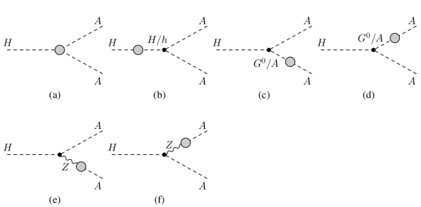
Figure 4: Generic diagrams contributing to the virtual corrections of $H\to AA$: vertex corrections (a) and corrections to the external legs (b)-(f).

The 1PI diagrams of the vertex corrections are displayed in Fig. 5. They consist of the 1PI diagrams given by the triangle diagrams with fermions, scalars and gauge bosons in the loops and by the diagrams containing four-particle vertices.

Figure 5: Generic diagrams contributing to the vertex corrections in $H\to AA$ with fermions $F$, scalar bosons $S$ and gauge bosons $V$ in the loops.

The counterterm contributions are given by the genuine vertex counterterm and by the counterterm insertions on the external legs, cf. Fig. 6. For the derivation of the latter we start from the bare Lagrangian involving the relevant trilinear Higgs self-couplings. With the coupling factors

$$g_{hAA} = \frac{1}{2M_{W}}\left[s_{\beta-\alpha}(2m_{A}^{2}-m_{h}^{2})+\frac{c_{\alpha+\beta}}{s_{2\beta}}\left(2m_{h}^{2}-\frac{2m_{12}^{2}}{s_{\beta}c_{\beta}}\right)\right]$$ (4.43)

$$g_{HG^{0}A} = -\frac{s_{\beta-\alpha}}{2M_{W}}(m_{A}^{2}-m_{H}^{2})$$ (4.44)

and $g_{HAA}$ defined in Eq. (4.41) it reads in terms of the bare fields denoted by the subscript $0$,

$${\cal L}_{\text{int}}^{HAA}=g\left[-\frac{g_{hAA}}{2!}h_{0}A_{0}A_{0}-\frac{g_{HAA}}{2!}H_{0}A_{0}A_{0}-g_{HG^{0}A}H_{0}G_{0}^{0}A_{0}\right]\,.$$ (4.45)

Replacing the bare fields by their renormalized ones and the corresponding wave function renormalization constants, the NLO expansion of the Lagrangian reads

$${\cal L}_{\text{int}}^{HAA}\stackrel{{\scriptstyle\text{NLO}}}{{\approx}}g\left[-\frac{g_{hAA}}{2!}\frac{\delta Z_{hH}}{2}-\frac{g_{HAA}}{2!}\left(\delta Z_{AA}+\frac{\delta Z_{HH}}{2}\right)-g_{HG^{0}A}\frac{\delta Z_{G^{0}A}}{2}\right]HAA\;.$$ (4.46)

Figure 6: Counterterm diagrams contributing to the NLO decay $H\to AA$.

The Feynman rule $\lambda_{\text{CT,WR}}^{HAA}$ for the counterterm contribution from the wave function renormalization is obtained by performing the functional derivatives with respect to the external renormalized fields,

$$\lambda_{\text{CT,WR}}^{HAA} = i\frac{\delta}{i\delta H}\frac{\delta}{i\delta A}\frac{\delta}{i\delta A}{\cal L}_{\text{int}}^{HAA}\;.$$ (4.47)

Together with the genuine vertex counterterm $\delta(g\cdot g_{HAA})$

$$\delta(g\cdot g_{HAA}) = g\Big{\{}g_{HAA}\left(\frac{\delta g}{g}-\frac{\delta M_{W}}{M_{W}}\right)$$ (4.48)

$$-\frac{1}{2M_{W}}\left[c_{\beta-\alpha}(2\delta m_{A}^{2}-\delta m_{H}^{2})+\frac{s_{\alpha+\beta}}{s_{2\beta}}\left(2\delta m_{H}^{2}-\frac{4}{s_{2\beta}}\delta m_{12}^{2}\right)\right]$$

$$-\frac{1}{2M_{W}}\left[s_{\alpha-\beta}(2m_{A}^{2}-m_{H}^{2})+\frac{2(c_{\alpha}s_{\beta}^{3}-s_{\alpha}c_{\beta}^{3})}{s_{2\beta}^{2}}\left(2m_{H}^{2}-\frac{4m_{12}^{2}}{s_{2\beta}}\right)+\frac{8c_{2\beta}s_{\alpha+\beta}m_{12}^{2}}{s_{2\beta}^{3}}\right]\delta\beta$$

$$-\frac{1}{2M_{W}}\left[-s_{\alpha-\beta}(2m_{A}^{2}-m_{H}^{2})+\frac{c_{\alpha+\beta}}{s_{2\beta}}\left(2m_{H}^{2}-\frac{4m_{12}^{2}}{s_{2\beta}}\right)\right]\delta\alpha\Big{\}}\;.$$

we obtain for the counterterm amplitude

$${\cal M}^{\text{CT}}_{HAA}=g\left[g_{hAA}\frac{\delta Z_{hH}}{2}+g_{HAA}\left(\delta Z_{AA}+\frac{\delta Z_{HH}}{2}\right)+g_{HG^{0}A}\delta Z_{G^{0}A}+\frac{1}{g}\delta(g\cdot g_{HAA})\right]\;.$$ (4.49)

The one-loop amplitude ${\cal M}_{HAA}^{\text{1loop}}$ of the decay $H\to AA$ consists of the amplitude built from the vertex corrections ${\cal M}_{HAA}^{\text{VC}}$ and of the counterterm amplitude,

$${\cal M}_{HAA}^{\text{1loop}}={\cal M}_{HAA}^{\text{VC}}+{\cal M}^{\text{CT}}_{HAA}\;.$$ (4.50)

With the LO amplitude ${\cal M}_{HAA}^{\text{LO}}$ we then obtain the NLO partial decay width as

$$\Gamma^{\text{NLO}}=\Gamma^{\text{LO}}+\frac{m_{H}}{32\pi}\sqrt{1-\frac{4m_{A}^{2}}{m_{H}^{2}}}\,2\,\mbox{Re}\left[({\cal M}_{HAA}^{\text{LO}})^{*}{\cal M}_{HAA}^{\text{1loop}}\right]\;.$$ (4.51)

The counterterm $\delta m_{12}^{2}$ is fixed by the process-dependent renormalization condition

$$\Gamma^{\text{LO}}(H\to AA)\stackrel{{\scriptstyle!}}{{=}}\Gamma^{\text{NLO}}(H\to AA)\;.$$ (4.52)

This leads to the counterterm definition

$$\delta m_{12}^{2}=-\frac{vs_{2\beta}^{2}}{4s_{\alpha+\beta}}\mbox{Re}\left[{\cal M}_{HAA}^{\text{VC}}+({\cal M}^{\text{CT}}_{HAA})_{\delta m_{12}^{2}=0}\right]\;.$$ (4.53)

The additional diagrams that must be taken into account when the alternative tadpole scheme is a applied are displayed in Fig. 7. Note that the overall NLO amplitude is invariant under a change of the tadpole schemes, provided the angular counterterms are determined in a process-dependent way.

Figure 7: Additional vertex diagrams in the alternative tadpole scheme contributing to the decay $H\to AA$.

4.3 Gauge (In)dependence of the NLO amplitude

As the expressions for the vertex corrections and counterterms are quite involved we limit our discussion here to a qualitative level. The quantitative corroboration of our statements will be presented in the numerical analysis.

In case the standard tadpole scheme is applied the computation of the NLO decay amplitude in the general $R_{\xi}$ gauge reveals that the residual amplitude ${\cal M}$ with the counterterms

$$\delta p\equiv\delta\alpha\;,\;\delta\beta\mbox{ and }\delta m_{12}^{2}$$ (4.54)

set to zero exhibits a UV-divergent gauge dependence,

$$\underline{\mbox{\it Standard tadpole scheme:}}\qquad{\cal M}_{H\to hh}|_{\text{NLO},\xi,\delta p=0}^{\text{standard}}\neq 0\;\to\infty\;.$$ (4.55)

This divergence can only be cancelled by the angular counterterms, so that in this scheme they necessarily have to be gauge dependent. Renormalizing $\alpha$ and $\beta$ through the process-dependent scheme cancels all UV-divergent gauge-dependent parts. The remaining UV-divergent gauge-independent terms are then cancelled by $\delta m_{12}^{2}$. It can be defined either via an $\overline{\mbox{MS}}$ condition or through the process $H\to AA$. The overall NLO amplitude will finally be gauge independent as it should be.

Applying the alternative tadpole scheme instead leads to the cancellation of the UV-divergent gauge-dependent parts within the residual amplitude, i.e.

$$\underline{\mbox{\it Alternative tadpole scheme:}}\qquad{\cal M}_{H\to hh}|_{\text{NLO},\xi,\delta p=0}^{\text{tad}}=0\;.$$ (4.56)

The angular counterterms in turn can then be defined gauge-independently. The unambiguous gauge-independent definition of the angular counterterms is achieved through the pinched scheme or the definition via a physical process. The counterterm for $m_{12}^{2}$ is gauge-independent irrespective of the tadpole scheme and can be renormalized in the $\overline{\mbox{MS}}$ or the process-dependent scheme.

We can summarize that a gauge-independent decay amplitude for the process $H\to hh$ is achieved by applying the following renormalization schemes for the angular counterterms:

tadpole treatment	$\delta\alpha,\delta\beta$	gauge dependence $\delta\alpha$, $\delta\beta$
standard tadpole scheme	process dependent	gauge dependent
alternative tadpole scheme	pinched scheme	gauge independent
	process dependent

Throughout the calculation we employ the alternative tadpole scheme. This guarantees the manifestly gauge-independent renormalization of the counterterms. It is furthermore indispensable for a gauge-independent decay amplitude if the angular counterterms are not obtained via a physical process.

Concerning a scheme with process-dependent counterterm definitions, note, that the results for the NLO decay widths are the same in the standard and in the alternative tadpole scheme. A change of the tadpole scheme leaves the total NLO amplitude invariant, it only moves around the gauge dependencies between the various building blocks, so that in the alternative tadpole scheme the counterterms become gauge independent.

5 Numerical analysis

The NLO EW corrections to the Higgs decay width $H\to hh$ have been performed in two independent calculations and all results have been cross-checked against each other. They agree within numerical errors. The two computations use the Mathematica package FeynArts 3.9 and 3.7 [64, 65], respectively, for the generation of the LO and NLO amplitudes in the general $R_{\xi}$ gauge. For this, the model file for the CP-conserving 2HDM was used, which is already implemented in the package. The additionally needed tadpole and self-energy amplitudes for the definition of the counterterms and wave function renormalization constants have been generated in the general $R_{\xi}$ gauge. For the contraction of the Dirac matrices and the expression of the results in terms of scalar loop integrals FeynCalc 8.2.0 [66, 67] has been applied in one calculation and FormCalc 8.1 [68] in the other. The C++ library LoopTools 2.12 and 2.9 [68], respectively, has been used for the numerical evaluation of the dimensionally regularized [69, 70] integrals.

Our numerical evaluation has been performed with the following input parameters. The fine structure constant $\alpha$ is taken at the $Z$ boson mass scale [71],

$$\alpha(M_{Z}^{2})=\frac{1}{128.962}\;,$$ (5.57)

and for the massive gauge boson masses we use [71, 72]

$$M_{W}=80.385\mbox{ GeV}\qquad\mbox{and}\qquad M_{Z}=91.1876\mbox{ GeV}\;.$$ (5.58)

The lepton masses are chosen as [71, 72]

$$m_{e}=0.510998928\mbox{ MeV}\;,\quad m_{\mu}=105.6583715\mbox{ MeV}\;,\quad m_{\tau}=1.77682\mbox{ GeV}\;,$$ (5.59)

and the light quark masses, following [73], are set to

$$m_{u}=100\mbox{ MeV}\;,\quad m_{d}=100\mbox{ MeV}\;,\quad m_{s}=100\mbox{ MeV}\;.$$ (5.60)

The leptons and light quarks have only a small influence on the results. For consistency with the ATLAS and CMS analyses the following OS value for the top quark mass is taken,

$$m_{t}=172.5\mbox{ GeV}\;,$$ (5.61)

as recommended by the LHC Higgs Cross Section Working Group (HXSWG) [72, 74]. For the charm and bottom quark OS masses we use [72]

$$m_{c}=1.51\mbox{ GeV}\qquad\mbox{and}\qquad m_{b}=4.92\mbox{ GeV}\;.$$ (5.62)

As we do not include CP violation the CKM matrix is real, with the CKM matrix elements given by [71]

$$V_{\text{CKM}}=\left(\begin{array}[]{ccc}V_{ud}&V_{us}&V_{ub}\\ V_{cd}&V_{cs}&V_{cb}\\ V_{td}&V_{ts}&V_{tb}\end{array}\right)=\left(\begin{array}[]{ccc}0.97427&0.22536&0.00355\\ -0.22522&0.97343&0.0414\\ 0.00886&-0.0405&0.99914\end{array}\right)\;.$$ (5.69)

Finally for the SM-like Higgs mass value, denoted by $m_{H^{\text{SM}}}$, we take the most recent combined value from ATLAS and CMS [75],

$$m_{H^{\text{SM}}}=125.09\mbox{ GeV}\;.$$ (5.70)

In the 2HDM both the heavier and the lighter of the two CP-even Higgs bosons can play the role of the SM-like Higgs boson, depending on the chosen parameter set. In our investigated cases it is the lighter of the CP-even Higgs bosons, $h$, that corresponds to $H^{\text{SM}}$.

For the numerical analysis only those 2HDM parameter sets have been taken into account that have not yet been excluded by experimental and the most relevant theoretical constraints. These parameter points have been obtained by scans performed in the 2HDM parameter space with the tool ScannerS [76]. It checks if the chosen CP-conserving vacuum represents the global minimum [77], if the 2HDM potential is bounded from below[78] and if tree-level unitarity holds [79, 80]. The consistency with the electroweak precision constraints [81, 82, 83, 84, 85, 86, 87] is assumed to be fulfilled if the $S,T$ and $U$ variables [81] predicted by the 2HDM are within the 95% ellipsoid centered on the best fit point to the EW data. Loop processes with charged Higgs bosons induce indirect constraints that depend on $\tan\beta$ via the charged Higgs coupling to the fermions. They dominantly stem from $B$ physics observables [88, 89, 90] and the measurement of $R_{b}$ [91, 92, 93, 94]. In our analysis we take the most recent bound of $m_{H^{\pm}}\raisebox{-3.69899pt}{~{}\shortstack{$>$ \\ [-0.07cm] $\sim$}}~{}480$ GeV for the type II and flipped 2HDM [62]. Note, that the results from LEP [95] and the LHC [96, 97] require the charged Higgs mass to be above ${\cal O}(100\mbox{ GeV})$ depending on the model type. For the check of the compatibility with the LHC Higgs data ScannerS uses the Higgs production cross sections through gluon fusion and $b$-quark fusion at NNLO QCD, which are obtained from an interface with SusHi [99]. The remaining production cross sections are taken at NLO QCD [73], and the 2HDM Higgs decays are computed with HDECAY [100, 101]. The EW corrections are consistently neglected in the computation of these processes as they have not been provided for the 2HDM so far. The program HiggsBounds [102, 103, 104] is used for the check of the exclusion limits and HiggsSignals [105] is used to test the compatibility with the observed signal for the 125 GeV Higgs. Further details can be found in [106]. All results shown in the following analysis are for the 2HDM type II.

For the numerical analysis we exploit three different sets of parameter points that are distinguished with respect to their Higgs spectra but that all fulfill the above listed experimental and theoretical constraints:

• The parameter sets are chosen such that the decay $H\to hh$ is kinematically possible, hence

  $${\mbox{\it Condition (i): }}\quad M_{H}\stackrel{{\scriptstyle!}}{{\geq}}2M_{h}\;.$$ (5.71)

• The parameter sets are chosen such that the decay $H\to hh$ is kinematically possible. Additionally, we require the heavy Higgs boson masses to maximally deviate by $\pm 5\%$ from $M$, with $M^{2}\equiv m_{12}^{2}/(s_{\beta}c_{\beta})$. We hence have

  Condition (ii): $$M_{H}\stackrel{{\scriptstyle!}}{{\geq}}2M_{h}\qquad\qquad\mbox{ and }$$ (5.73)

  $$m_{\phi_{\text{heavy}}}\stackrel{{\scriptstyle!}}{{=}}M\pm 5\%\;,\;\mbox{ with }m_{\phi_{\text{heavy}}}\in\{m_{H},m_{A},m_{H^{\pm}}\}\;.$$

  In these scenarios the non-SM Higgs bosons are approximately mass degenerate and of the order of the ${\mathbb{Z}}_{2}$ breaking scale.

• The conditions for the parameter sets chosen here are that both the decay $H\to hh$ and the decay $H\to AA$ are kinematically possible, i.e.

  $${\mbox{\it Condition (iii): }}\quad M_{H}\stackrel{{\scriptstyle!}}{{\geq}}2M_{h}\qquad\mbox{and}\qquad M_{H}\stackrel{{\scriptstyle!}}{{\geq}}2M_{A}\;.$$ (5.74)

As we have seen in subsection 4.1 the decay $H\to hh$ depends through the Higgs self-coupling $\lambda_{Hhh}$ on both mixing angles $\alpha$ and $\beta$ and on the soft $\mathbb{Z}_{2}$ breaking parameter $m_{12}^{2}$. This process hence allows us to study the numerical stability of the renormalization schemes for the mixing angles but in particular also of the mass parameter $m_{12}^{2}$. The possible renormalization schemes for the angular counterterms are denoted as follows,

$$\begin{array}[]{lll}\mbox{proc}&:&\quad\mbox{process-dependent}\\ p_{\star}^{c,o}&:&\quad p_{\star}\mbox{ tadpole-pinched},\;\delta\beta^{(1)}\mbox{ ('$c$') or }\delta\beta^{(2)}\mbox{ ('$o$')}\\ \mbox{pOS}^{c,o}&:&\quad\mbox{on-shell tadpole-pinched},\;\delta\beta^{(1)}\mbox{ ('$c$') or }\delta\beta^{(2)}\mbox{ ('$o$')}\;.\end{array}$$ (5.78)

As explained above, the process-dependent renormalization for $\alpha$ proceeds through the decay $H\to\tau\tau$ and the one for $\beta$ exploits $A\to\tau\tau$. In the tadpole-pinched schemes, $p_{\star}$ or pOS, $\beta$ can be renormalized through the charged sector, with the counterterm denoted by $\delta\beta^{(1)}$, or through the CP-odd sector, with the counterterm given by $\delta\beta^{(2)}$. For $m_{12}^{2}$ we adopt the two schemes

$$\begin{array}[]{lll}\mbox{proc}&:&\quad\mbox{process-dependent via }H\to AA\mbox{ and}\\ \overline{\mbox{MS}}&:&\quad\mbox{modified minimal subtraction scheme}\;.\end{array}$$ (5.81)

We investigate the size of the NLO corrections by defining

$$\Delta\Gamma\equiv\frac{\Gamma^{\text{NLO}}-\Gamma^{\text{LO}}}{\Gamma^{\text{LO}}}\;.$$ (5.82)

This ratio measures the relative size of the NLO corrections compared to the LO decay width. We start by investigating the impact of the angular renormalization schemes on the NLO corrections to the Higgs-to-Higgs decays. To this end we show in Fig. 8 for all parameter sets of $(i)$ the relative NLO corrections $\Delta\Gamma^{H\to hh}$ as a function of the LO width for all possible angular schemes defined in (5.78). For $\beta$ both possible renormalization choices through the charged and through the CP-odd sector have been applied in the tadpole-pinched schemes. For $\delta m_{12}^{2}$ the $\overline{\mbox{MS}}$ scheme has been applied with the renormalization scale set to $\mu_{R}=2m_{h}$. As can be inferred from the plot, the relative corrections can be huge. Discarding the region for small LO widths, where $\Delta\Gamma^{H\to hh}$ diverges, we have relative corrections of up to about 400% (not shown in the plot) in the process dependent scheme and of up to about 200% for the tadpole-pinched schemes. Note that we cut the plot at $\Delta\Gamma^{Hhh}=-100\%$ in order to avoid negative widths.

The appearance of huge corrections is not necessarily due to numerical instability. It is rather the non-decoupling effects, generically arising in the 2HDM [32, 107], that blow up the NLO corrections. This shall be explained in the following. For the decay $H\to hh$ being kinematically possible large enough $H$ masses are needed. As can be read off from Eq. (2.53), heavy masses can either be obtained through a large mass parameter $M$ or through the VEVs. They enter the mass relation with a coefficient proportional to a linear combination of the Higgs potential couplings $\lambda_{i}$. In the decoupling limit we have $c_{\phi}^{2}M^{2}\gg f(\lambda_{i})v^{2}$, and the spectrum effectively consists of heavy Higgs bosons whose masses are given by the scale $c_{\phi_{\text{heavy}}}M$ independently of the $\lambda_{i}$, and of one light resonance that represents the SM-like Higgs boson. The trilinear and quartic scalar couplings controlled by $\lambda_{i}$ are comparatively small and all loop effects due to the heavier Higgs bosons vanish in the limit $m_{\phi_{\text{heavy}}}^{2}\to\infty$ because of the decoupling theorem [108]. This situation corresponds to the decoupling limit of the MSSM, where supersymmetry requires the couplings $\lambda_{i}$ to be replaced by the gauge couplings $g$ and $g^{\prime}$ and where heavy masses can only be obtained through a large mass scale $M$ usually chosen to be the pseudoscalar mass $M_{A}$. In the opposite case, the strong coupling regime, we have $c_{\phi_{\text{heavy}}}^{2}M^{2}\raisebox{-3.69899pt}{~{}\shortstack{$<$ \\ [-0.07cm] $\sim$}}~{}f(\lambda_{i})\,v^{2}$ for at least one of the non-SM-like Higgs bosons, and large mass values can only be obtained for large couplings $\lambda_{i}$. The decoupling theorem does not apply and the radiative corrections of the heavy Higgs bosons develop a power-like behaviour in $m_{\phi_{\text{heavy}}}$, also known as non-decoupling effects [109, 110, 111, 112, 113, 114, 115, 116, 117, 118]. They grow proportional to $m_{\phi_{\text{heavy}}}^{4}$ [32, 107]. The huge corrections in Fig. 8 are due to this power law for scenarios with heavy non-SM Higgs bosons.

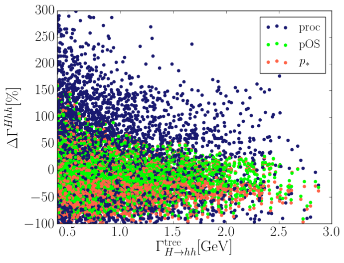
Figure 8: Scatter plot for the relative NLO corrections to $H\to hh$ for all parameter points passing the theoretical and experimental constraints and fulfilling the kinematic condition $(i)$, as a function of the LO width; shown for various angular renormalization schemes: process-dependent (blue), pOS tadpole-pinched (green), $p_{\star}$ tadpole-pinched (red); $m_{12}^{2}$ has been $\overline{\mbox{MS}}$ renormalized with $\mu_{R}=2m_{h}$. Scenarios leading to negative widths for one of the renormalization schemes have been discarded, and we have cut at 300% for positive corrections.

From the above discussion it becomes clear that for a meaningful discussion of the numerical stability of the different renormalization schemes we have to separate the two effects: huge corrections due to large couplings $\lambda_{i}$ and corrections that are blown-up due to numerical instability of the chosen renormalization scheme. We therefore investigate the relative NLO corrections for the parameter set $(ii)$ where we require all non-SM heavy Higgs masses to lie within 5% around the mass scale $M$ set by the soft $\mathbb{Z}_{2}$ breaking mass parameter. In this limit, the loop effects of the heavy particles are expected to decouple. However, even if Eq. (5.73) is fulfilled, the decoupling does not necessarily take place. It is found to be impossible, in fact, in the limit $s_{\alpha+\beta}\to 1$. This limit is referred to as the wrong sign limit as for the 2HDM type II (and F) it implies a relative minus sign in the couplings of the SM-like Higgs boson to down-type fermions with respect to its couplings to massive gauge bosons (and up-type fermions) [106, 119, 120, 121]. In Ref. [119] it was shown that non-decoupling properties inevitably arise for $s_{\beta+\alpha}\to 1$ in the 2HDM. The non-decoupling of charged Higgs contributions in the loop induced $h\gamma\gamma$ coupling was also discussed in [12, 122, 123].

In order to examine the non-decoupling properties of the loop contributions to $H\to hh$ we focus on the trigonometric relations relevant for the involved Higgs couplings. Two limiting cases are of interest, given by $s_{\beta-\alpha}\approx 1$ and $s_{\beta-\alpha}<1$. While $s_{\beta-\alpha}\to 1$ corresponds to the SM limit, in the wrong sign regime significant deviations from this limit are still compatible with LHC data. Thus it was shown in [106, 120, 121] that values of $s_{\beta-\alpha}\approx 0.55$ (0.62) are compatible with the LHC Higgs data at 3 (2)$\sigma$ and additionally fulfill the other constraints tested by ScannerS. Relatively small values of $s_{\beta-\alpha}$, however, require significant contributions from the second term in Eq. (2.53), given by $f(\lambda_{i})v^{2}$, even if $m_{H}^{2}\approx M^{2}$, in order to acquire a sufficiently large $m_{H}$ for the decay $H\to hh$ to take place. This, however, drives us back to the non-decoupling limit.

Also in the limit $s_{\beta-\alpha}\to 1$, corresponding to SM-like $h$ couplings to the massive gauge bosons, the trilinear coupling $\lambda_{Hhh}$ can become large in the wrong sign limit. Analogous to the non-decoupling of the charged Higgs contribution in the decay $h\to\gamma\gamma$ studied in Ref. [119], also the other heavy Higgs bosons $H$ and $A$ exhibit a non-decoupling behaviour in the wrong sign limit. In order to show this, we consider the ratio $\lambda_{HHh}/m_{H}^{2}$, which plays a role in the EW corrections to $H\to hh$. We analyze this ratio for both the correct and the wrong sign regime in the limit $s_{\beta-\alpha}\to 1$, where $m_{H}^{2}\approx M^{2}$. In the wrong sign regime, where $s_{\beta+\alpha}\to 1$, $t_{\beta}$ has to be large in order to come close to the SM limit. We thus obtain

$$\frac{\lambda_{HHh}}{m_{H}^{2}} = -\frac{1}{m_{H}^{2}v}\frac{s_{\beta-\alpha}}{s_{2\beta}}\left[s_{2\alpha}(2m_{H}^{2}+m_{h}^{2})-M^{2}(3s_{2\alpha}+s_{2\beta})\right]$$ (5.87)

$$\approx \frac{1}{v}\frac{s_{\beta-\alpha}}{s_{2\beta}}[s_{2\alpha}+s_{2\beta}]+{\cal O}\left(\frac{m_{h}^{2}}{vm_{H}^{2}}\right)$$

$$= \frac{1}{v}s_{\beta-\alpha}\left(1-\frac{s_{\beta-\alpha}-c_{\beta-\alpha}t_{\beta}}{s_{\beta-\alpha}+c_{\beta-\alpha}t_{\alpha}}\right)+{\cal O}\left(\frac{m_{h}^{2}}{vm_{H}^{2}}\right)$$

$$\left\{\begin{array}[]{cll}\stackrel{{\scriptstyle s_{\beta-\alpha}\to 1}}{{\approx}}&0&\;\mbox{ correct sign limit}\\ \stackrel{{\scriptstyle{\scriptsize\begin{array}[]{l}s_{\beta+\alpha}\to 1,\\ t_{\beta}\to\infty\end{array}}}}{{\approx}}&2/v&\;\mbox{ wrong sign limit}\end{array}\right.+{\cal O}\left(\frac{m_{h}^{2}}{vm_{H}^{2}}\right)\;.$$

As can be inferred from Eq. (5.87) the ratio $\lambda_{HHh}/m_{H}^{2}$ approaches a constant value in the wrong sign regime so that the heavy Higgs loop contributions do not decouple for $m_{H}^{2}\to\infty$. In contrast, in the correct sign limit the ratio vanishes and the decoupling of heavy $H$ loop effects takes place. Analogously, the ratio $\lambda_{Hhh}/m_{H}^{2}$ yields a constant value in the wrong sign regime and prevents a decoupling of heavy loop particle contributions. The same holds for $\lambda_{hAA}/m_{A}^{2}$ where we find

$$\frac{\lambda_{hAA}}{m_{A}^{2}} = \frac{2}{v}c_{\beta-\alpha}\left(\frac{1}{t_{\beta}}-t_{\beta}\right)+{\cal O}\left(\frac{m_{h}^{2}}{vm_{A}^{2}}\right)$$ (5.92)

$$\left\{\begin{array}[]{cll}\stackrel{{\scriptstyle s_{\beta-\alpha}\to 1}}{{\approx}}&0&\;\mbox{ correct sign limit}\\ \stackrel{{\scriptstyle{\scriptsize\begin{array}[]{l}s_{\beta+\alpha}\to 1,\\ t_{\beta}\to\infty\end{array}}}}{{\approx}}&-2/v&\;\mbox{ wrong sign limit}\end{array}\right.+{\cal O}\left(\frac{m_{h}^{2}}{vm_{A}^{2}}\right)\;.$$

This non-decoupling behaviour in the wrong sign regime explains why even in the case where the heavy Higgs boson masses are controlled by

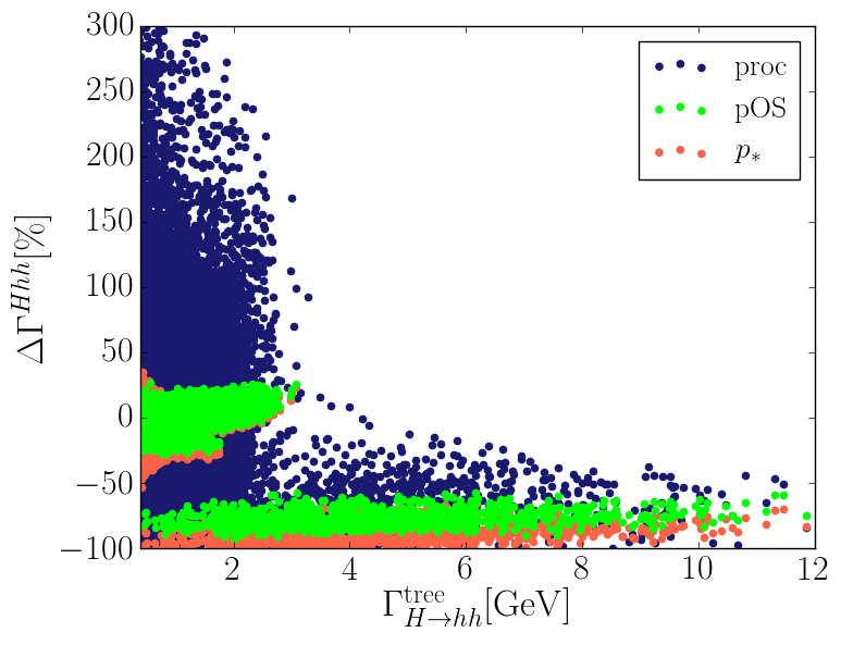
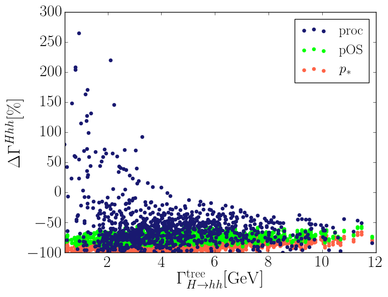
Figure 9: Scatter plot for the relative NLO corrections to $H\to hh$ for all parameter points passing the theoretical and experimental constraints and fulfilling the kinematic condition $(ii)$, as a function of the LO width; shown for various angular renormalization schemes: process-dependent (blue), pOS tadpole-pinched (green), $p_{\star}$ tadpole-pinched (red); $m_{12}^{2}$ has been $\overline{\mbox{MS}}$ renormalized with $\mu_{R}=2m_{h}$. Scenarios leading to negative widths for one of the renormalization schemes have been discarded, and we have cut at 300% for positive corrections. Left: all points, right: only those with $\sin\alpha>0$, corresponding to the wrong sign regime.

the mass parameter $M$ the loop effects do not decouple and give rise to large radiative corrections. This behaviour is shown in the following plots. In Fig. 9 (left) we first display for all points of parameter set $(ii)$ that pass the theoretical and experimental constraints the relative NLO corrections as a function of the LO width for the process-dependent and the two tadpole-pinched schemes in the angular renormalization. For $m_{12}^{2}$ $\overline{\text{MS}}$ renormalization has been applied at $\mu_{R}=2m_{h}$. Although our involved heavy Higgs masses are due to a large value of $M$, we observe huge relative corrections of up to 300% and larger. Note that in the plot we cut at -100% in order to avoid negative widths. Following our considerations on the decoupling behaviour of loop corrections in the SM-limit, we now divide our parameter points into those of the wrong sign regime, where $s_{\beta+\alpha}\approx 1$, and those of the correct sign regime with $s_{\beta-\alpha}\approx 1$. We used the sign of $s_{\alpha}$ as discriminator between the two regimes, collecting the parameter sets with $s_{\alpha}>0$ for the former and the ones with $s_{\alpha}<0$ for the latter case. This leads to Fig. 9 (right) which displays the relative corrections for the wrong sign regime and Fig. 10 for the correct sign regime. We show results for all applied renormalization schemes, discard points with small LO widths and cut at +300% and -100%, the latter to avoid negative widths. As expected, in Fig. 9 (right), despite the fact that all heavy 2HDM Higgs masses have been chosen within 5% around $M$, the corrections can be huge, reaching up to 300% and larger (not shown in the plot). The plot shows that in the tadpole pinched schemes for the displayed parameter points the relative corrections for all scenarios are within about -50% to -100%. In the process-dependent scheme we can have rather small corrections, but also huge corrections, exceeding largely those of the process-independent schemes. Large corrections as found for the tadpole pinched schemes are to be expected for significant coupling strengths as involved in the NLO diagrams here. This is confirmed by the explicit verification that in this non-decoupling regime the pure vertex corrections become large. The small corrections found for some scenarios in the process-dependent scheme are due to accidental cancellations between the various terms contributing at NLO and not because of more numerical stability in this renormalization scheme. This is why we observe here also huge corrections of up to 300% and beyond while this is not the case for the process-independent schemes. In order to be able to draw more conclusive statements on the numerical stability, corrections beyond the one-loop level would have to be calculated in this regime of strong coupling constants. This is beyond the scope of this paper.

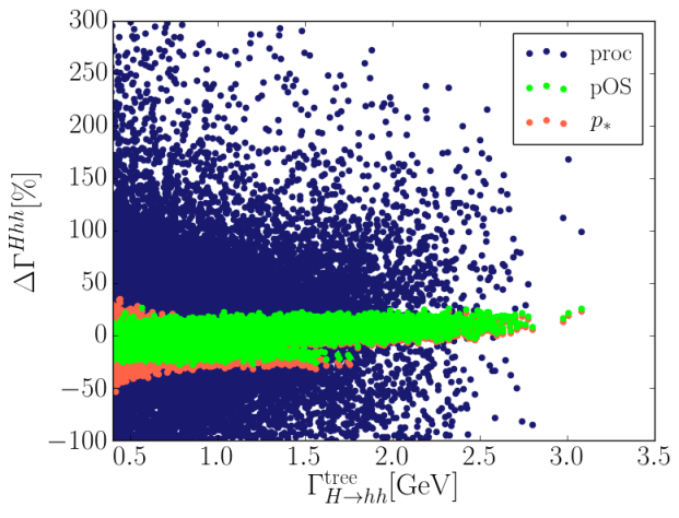
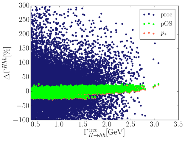
Figure 10: Same as Fig. 9 but only with points featuring scenarios in the correct sign limit, i.e. $\sin\alpha<0$. Left: all schemes, right: without $\beta$ renormalization in the $p_{\star}^{o}$ scheme, see text.

Taking into account only scenarios in the correct sign limit, we are left with Fig. 10, where we cut on scenarios leading to relative corrections beyond $+300$% and $-100$%, respectively, and discarded those with small LO widths. As explained above in detail, we are now truly in the decoupling limit. This is reflected by the plot. Since the involved trilinear couplings are not as large as in the wrong sign regime, for the process-independent renormalization schemes the relative NLO corrections have become considerably smaller as compared to the wrong sign case. Also of course, the LO widths are smaller. Having excluded scenarios with enhanced corrections due to non-decoupling, we can now proceed to investigate the numerical stability of the applied schemes. Inspecting Fig. 10 (left), we see that the corrections in the tadpole-pinched schemes all lie between about -60 and +40%. The process-dependent renormalization on the other hand induces much larger corrections, of the order of up to 300% and larger. While again we can also have small corrections in the process-dependent scheme, this is due to accidental cancellations and not a sign of numerical stability. This statement is underlined by the fact that the corrections in this scheme can become huge as well, whereas in the process-independent schemes they do not exceed $-60$%. In Fig. 10 (left) we furthermore see a difference between the pOS and the $p_{\star}$ tadpole-pinched scheme. For small LO widths the relative NLO corrections in the $p_{\star}$ tadpole-pinched scheme increase more quickly. This behaviour can be traced back to the appearance of the top resonance in the $G^{0}A$ self-energy encountered in the $\beta$ renormalization through the CP-odd Higgs sector, i.e. in $\delta\beta^{(2)}$. For masses $m_{A}^{2}/2=4m_{t}^{2}$ the diagram shown in Fig. 11 becomes resonant. This requires relatively light pseudoscalar masses of about 488 GeV. The tail of this effect is, however, still visible for masses up to $m_{A}\approx 700$ GeV. In the renormalization through the charged sector no self-energy diagrams with pure top loop contributions are encountered in the mixed $G^{\pm}H^{\pm}$ self-energy so that the counterterm $\delta\beta^{(1)}$ is not affected by the top resonance. Note furthermore that the counterterm $\delta\beta^{(2)}$ in the pOS scheme would require $A$ masses as low as 350 GeV to hit the top resonance. These are not included in set $(ii)$ so that no resonant enhancement is visible in the pOS scheme.

Figure 11: Top loop diagram contributing to the mixed self-energy $\Sigma^{\text{tad}}_{G^{0}A}$ in the $\beta$ renormalization.

In Fig. 10 (right) we have excluded the $p_{\star}^{o}$ renormalization of $\delta\beta$ from the plot. As expected all tadpole-pinched schemes now show the same behaviour. For scenarios with light pseudoscalar masses the $\beta$ renormalization through the charged sector might therefore be preferable. From these investigations we furthermore conclude that the tadpole-pinched schemes are numerically stable and can hence be advocated as renormalization schemes for the mixing angles that are numerically stable, gauge independent and process independent. This confirms our findings of [18] in a process involving a coupling that has a complicated dependence on $\alpha$ and $\beta$ so that the cancellation of huge tadpole contributions is non-trivial. Moreover, the plots show the good numerical behaviour of the $\overline{\mbox{MS}}$ scheme applied for $\delta m_{12}^{2}$. Independently of the discussion with respect to numerical stability we have seen that also in the tadpole-pinched schemes the corrections can be significant due to non-decoupling behaviour of the corrections. In these cases clearly higher order corrections have to be included in order to make reliable predictions. This is beyond the scope of this paper.

We finalize the discussion of the angular counterterms by examining a specific scenario in the decoupling limit. It is given by

$$\begin{array}[]{llll}\mbox{\it\text@underline{Scen1:}}&\;m_{H}=(671.05...803.12)\mbox{ GeV}\,,&\;m_{A}=700.13\mbox{ GeV}\,,&\;m_{H^{\pm}}=700.35\mbox{ GeV}\,,\\[2.84544pt] &\;\tan\beta=1.45851\,,&\;\alpha=-0.570376\,,&\;m_{12}^{2}=2.0761\cdot 10^{5}\mbox{ GeV}^{2}\end{array}$$ (5.95)

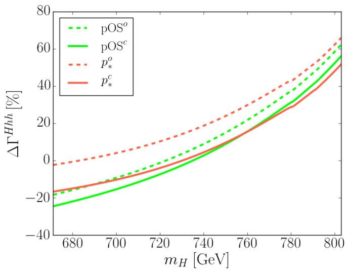
Figure 12: Relative NLO corrections to $H\to hh$ for angular renormalization in the tadpole-pinched schemes as defined in Eq. (5.78), with the 2HDM parameters given by Scen1, Eq. (5.95). $m_{12}^{2}$ has been $\overline{\mbox{MS}}$ renormalized with $\mu_{R}=2m_{h}$.

The chosen pseudoscalar Higgs mass is far above the top resonance so that no enhanced contributions in the $p_{\star}$ scheme are to be expected. Figure 12 displays the relative NLO correction to the decay $H\to hh$ for Scen1 as a function of the heavy Higgs boson mass $m_{H}$ for the renormalization of the mixing angles in the $p_{\star}$ and in the OS tadpole-pinched schemes. The angle $\beta$ has been renormalized both through the charged and through the CP-odd sector. We do not include the numerically unstable process-dependent renormalization. The kinks in the curves which appear independently of the renormalization scheme at $m_{H}\approx 781$ GeV and 791 GeV (not visible in the plot) are due to threshold effects in the scalar two-point function $B_{0}$ appearing in the counterterms. They are given by the following parameter configurations and counterterms

Kink	Kinematic point	Origin
1	$m_{H}(780.74\mbox{ GeV})=m_{H^{\pm}}(700.34\mbox{ GeV})+M_{W}$	$\delta Z_{hh},\delta Z_{HH},\delta Z_{Hh}$
2	$m_{H}(791.31\mbox{ GeV})=m_{A}(700.13\mbox{ GeV})+M_{Z}$	$\delta Z_{hh},\delta Z_{HH},\delta Z_{Hh}$

In the investigated mass range the LO width varies between 0.356 GeV at the lowest and 0.221 GeV at the highest $m_{H}$ value. As can be inferred from the plot, the relative corrections range between about -25% and +66% depending on $m_{H}$ and on the renormalization scheme. The corrections are large, but not numerically unstable. Comparing the results in the $p_{\star}^{c}$ and $p_{\star}^{o}$ scheme and those of the pOS^c and pOS^o scheme, the remaining theoretical uncertainty due to missing higher order corrections can be estimated based on a change of the renormalization scheme for $\beta$. The $p_{\star}$ scheme is more affected by the change of the renormalization scheme and induces an estimated theoretical uncertainty which varies between about 17% and 9% from the lower to the upper $m_{H}$ range. The residual theoretical uncertainty can also be estimated from the scale change by comparing the pOS^o with the $p_{\star}^{o}$ scheme on the one hand and pOS^c with the $p_{\star}^{c}$ scheme on the other hand. In the lower mass range the $\beta$ renormalization through the CP-odd sector suffers more from a change of the renormalization scale than the one through the charged Higgs sector. For the former the theoretical uncertainty is estimated to be about 20% here. At $m_{H}=803$ GeV for both schemes the uncertainties are similar with about 2-3%. Note that with growing $m_{H}$ the scenario departs more and more from the decoupling regime which is reflected in the increase of the NLO corrections.

So far we have used the renormalization scale $\mu_{R}=2m_{h}$ in the $\overline{\text{MS}}$ renormalization of $\delta m_{12}^{2}$. This scale choice is justified by Fig. 13. It shows the relative NLO corrections for the parameter points of set $(i)$ with $m_{12}^{2}$ $\overline{\mbox{MS}}$ renormalized at three different renormalization scales, given by $\mu_{R}=m_{H}$, $m_{h}$ and $2m_{h}$. Scenarios with small LO widths have been discarded, and we have cut the relative negative and positive corrections at -100% and 300%, respectively. The angles have been renormalized in the OS tadpole-pinched scheme.

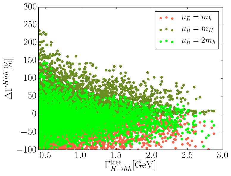
Figure 13: Scatter plot for the relative NLO corrections to $H\to hh$ for all parameter points passing the theoretical and experimental constraints and fulfilling the kinematic condition $(i)$, as a function of the LO width; shown for three different renormalization scales in the $\overline{\mbox{MS}}$ renormalized $m_{12}^{2}$: $\mu_{R}=m_{h}$ (red), $m_{H}$ (dark green) and $2m_{h}$ (light green); angles are pOS tadpole-pinched renormalized. Scenarios with negative NLO widths have been excluded, and the relative positive corrections have been cut at 300%.

As can be inferred from the plot, $\mu_{R}=2m_{h}$ yields the smallest corrections and is hence the recommended scale among the three.

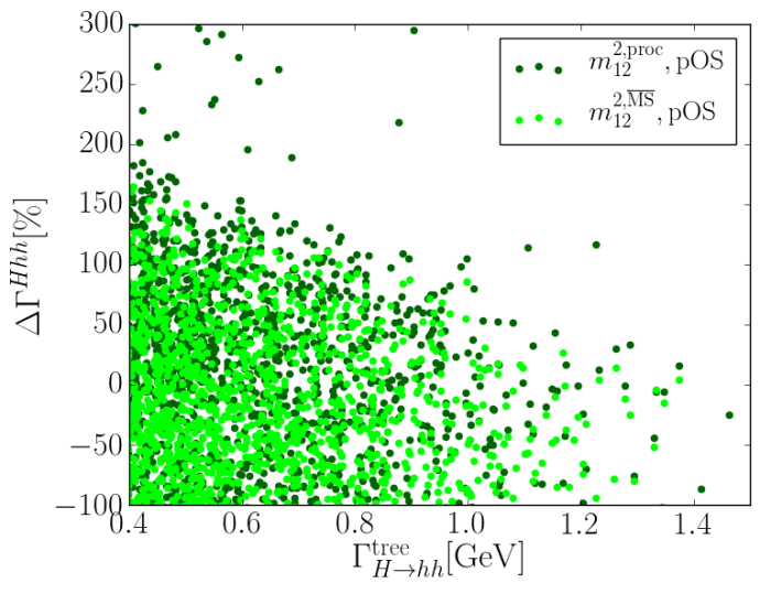
Figure 14: Scatter plot for the relative NLO corrections to $H\to hh$ for all parameter points passing the theoretical and experimental constraints and fulfilling the kinematic condition $(iii)$, as a function of the LO width; shown for the process-dependent renormalization of $m_{12}^{2}$ (dark green) and $\overline{\mbox{MS}}$ renormalization with $\mu_{R}=2m_{h}$. The angles have been renormalized in the pOS scheme. Scenarios with negative NLO widths have been excluded, and the relative positive corrections have been cut at 300%.

We now turn to the investigation of the process-dependent renormalization of $m_{12}^{2}$. For this purpose we use the parameter points of set $(iii)$ for which $H\to AA$ decays are kinematically allowed. Clearly, here we are not in the decoupling regime any more due to the mass hierarchy among the heavy non-SM Higgs bosons, so that large radiative corrections are to be expected. This is confirmed by Fig. 14 which shows the relative NLO corrections to the decay width $H\to hh$ as a function of the LO width for all points fulfilling condition (5.74) in accordance with the experimental and theoretical constraints. It compares the renormalization of $m_{12}^{2}$ through the process $H\to AA$ with the one in the $\overline{\mbox{MS}}$ scheme with $\mu_{R}=2m_{h}$. In both cases the mixing angles are renormalized in the pOS scheme. Due to the large involved couplings the corrections are found to be extremely large. In the $\overline{\mbox{MS}}$ scheme the corrections are restricted to values within about -300 and 150% discarding small LO widths. Corrections of this size can also be found in the process-dependent scheme, due to accidental cancellations among the various NLO terms. However, there are also scenarios yielding much larger relative corrections with values beyond 600% (not visible in the plot). In conclusion, the $\overline{\mbox{MS}}$ scheme is the preferable scheme for $m_{12}^{2}$ due to its better numerical stability that has been verified in the investigations in the decoupling regime. Again, of course, independent of the question of numerical stability, the overall large corrections also in the process-independent schemes call for the inclusion of higher order corrections that are beyond the scope of this paper.

6 Conclusions

We investigated the renormalization of the mass parameter $m_{12}^{2}$, which softly breaks the $\mathbb{Z}_{2}$ symmetry imposed on the 2HDM Higgs potential. The impact of the renormalization through the $\overline{\mbox{MS}}$ scheme and through a process-dependent definition via the decay $H\to AA$ was analyzed in the sample decay $H\to hh$. While the process-dependent scheme cannot be tested in the decoupling regime and hence a statement on its numerical stability is prevented by huge radiative corrections, our analysis still indicates an unfavourable numerical behaviour of the process-dependent scheme when compared to the $\overline{\mbox{MS}}$ scheme. The latter behaves better in the regime where the loop corrections are dominated by strong coupling contributions and the higher order corrections are hence parametrically enhanced. Furthermore, it has proven good numerical properties in the decoupling limit. The Higgs decay into lighter Higgs pairs also gave us the opportunity to reconfirm the good properties found previously in the tadpole-pinched renormalization scheme for the mixing angles $\alpha$ and $\beta$. Based on our findings we propose for the renormalization of the 2HDM Higgs sector the application of the tadpole-pinched scheme for the mixing angles $\alpha$ and $\beta$ and the $\overline{\mbox{MS}}$ scheme for $m_{12}^{2}$. These schemes lead to manifestly gauge-independent counterterms, are process independent and numerically stable. In scenarios featuring light CP-odd Higgs bosons ($m_{A}\raisebox{-3.69899pt}{~{}\shortstack{$<$ \\ [-0.07cm] $\sim$}}~{}700$ GeV), the $p_{\star}^{o}$ scheme is less preferable, due to the impact of the top resonance on $\delta\beta$ in this scheme.

Acknowledgments

The authors acknowledge financial support from the DAAD project “PPP Portugal 2015” (ID: 57128671). Hanna Ziesche acknowledges financial support from the Graduiertenkolleg “GRK 1694: Elementarteilchenphysik bei höchster Energie und höchster Präzision”. We are indebted to Marco Sampaio for kindly providing us with 2HDM data sets.

References

- [1] CMS, V. Khachatryan et al., Phys. Rev. D92, 012004 (2015) [arXiv:1411.3441 [hep-ex]].
- [2] ATLAS, G. Aad et al., Eur. Phys. J. C75, 476 (2015) [1506.05669 [hep-ex]].
- [3] CMS, V. Khachatryan et al., Eur. Phys. J. C75, 212 (2015) [1412.8662 [hep-ex]].
- [4] ATLAS, G. Aad et al., Eur. Phys. J. C76, 6 (2016) [1507.04548 [hep-ex]].
- [5] ATLAS Collaboration, G. Aad et al., Phys.Lett. B716, 1 (2012) [1207.7214 [hep-ex]].
- [6] CMS Collaboration, S. Chatrchyan et al., Phys.Lett. B716, 30 (2012) [1207.7235 [hep-ex]].
- [7] J. F. Gunion, H. E. Haber, G. L. Kane, and S. Dawson, Front.Phys. 80, 1 (2000).
- [8] T. D. Lee, Phys. Rev. D8, 1226 (1973).
- [9] G. C. Branco et al., Phys. Rept. 516, 1 (2012) [1106.0034 [hep-ph]].
- [10] A. Barroso, P. M. Ferreira, R. Santos, M. Sher, and J. P. Silva, 1304.5225 [hep-ph].
- [11] P. M. Ferreira, R. Santos, M. Sher, and J. P. Silva, 1305.4587 [hep-ph].
- [12] B. Dumont, J. F. Gunion, Y. Jiang, and S. Kraml, Phys. Rev. D90, 035021 (2014) [1405.3584 [hep-ph]].
- [13] J. Bernon, B. Dumont, and S. Kraml, Phys. Rev. D90, 071301 (2014) [1409.1588 [hep-ph]].
- [14] B. Dumont, J. F. Gunion, Y. Jiang, and S. Kraml, (2014) [1409.4088 [hep-ph]].
- [15] S. P. Martin, Adv.Ser.Direct.High Energy Phys. 21, 1 (2010) [hep-ph/9709356].
- [16] S. Dawson, hep-ph/9712464.
- [17] A. Djouadi, Phys.Rept. 459, 1 (2008) [hep-ph/0503173].
- [18] M. Krause, R. Lorenz, M. Muhlleitner, R. Santos, and H. Ziesche, 1605.04853 [hep-ph].
- [19] A. Denner, L. Jenniches, J.-N. Lang, and C. Sturm, (2016) [1607.07352 [hep-ph]].
- [20] A. Djouadi, W. Kilian, M. Muhlleitner, and P. M. Zerwas, Eur. Phys. J. C10, 27 (1999) [hep-ph/9903229].
- [21] A. Djouadi, W. Kilian, M. Muhlleitner, and P. M. Zerwas, Eur. Phys. J. C10, 45 (1999) [hep-ph/9904287].
- [22] M. M. Muhlleitner, Higgs particles in the standard model and supersymmetric theories, PhD thesis, Hamburg U., 2000, hep-ph/0008127.
- [23] D. T. Nhung, M. Muhlleitner, J. Streicher, and K. Walz, JHEP 11, 181 (2013) [1306.3926 [hep-ph]].
- [24] J. M. No and M. Ramsey-Musolf, Phys. Rev. D89, 095031 (2014) [1310.6035 [hep-ph]].
- [25] A. Arhrib, P. M. Ferreira, and R. Santos, JHEP 03, 053 (2014) [1311.1520 [hep-ph]].
- [26] J. Baglio, O. Eberhardt, U. Nierste, and M. Wiebusch, Phys. Rev. D90, 015008 (2014) [1403.1264 [hep-ph]].
- [27] S. F. King, M. Muhlleitner, R. Nevzorov, and K. Walz, Phys. Rev. D90, 095014 (2014) [1408.1120 [hep-ph]].
- [28] V. Barger, L. L. Everett, C. B. Jackson, A. D. Peterson, and G. Shaughnessy, Phys. Rev. D90, 095006 (2014) [1408.2525 [hep-ph]].
- [29] N.-E. Bomark, S. Moretti, S. Munir, and L. Roszkowski, JHEP 02, 044 (2015) [1409.8393 [hep-ph]].
- [30] R. Costa, M. Muhlleitner, M. O. P. Sampaio, and R. Santos, JHEP 06, 034 (2016) [1512.05355 [hep-ph]].
- [31] R. Grober, M. Muhlleitner, and M. Spira, JHEP 06, 080 (2016) [1602.05851 [hep-ph]].
- [32] S. Kanemura, Y. Okada, E. Senaha, and C. P. Yuan, Phys. Rev. D70, 115002 (2004) [hep-ph/0408364].
- [33] J. Fleischer and F. Jegerlehner, Phys. Rev. D23, 2001 (1981).
- [34] J. M. Cornwall and J. Papavassiliou, Phys. Rev. D40, 3474 (1989).
- [35] J. Papavassiliou, Phys. Rev. D41, 3179 (1990).
- [36] G. Degrassi and A. Sirlin, Phys. Rev. D46, 3104 (1992).
- [37] J. Papavassiliou, Phys. Rev. D50, 5958 (1994) [hep-ph/9406258].
- [38] N. J. Watson, Phys. Lett. B349, 155 (1995) [hep-ph/9412319].
- [39] D. Binosi and J. Papavassiliou, Phys. Rev. D66, 111901 (2002) [hep-ph/0208189].
- [40] D. Binosi and J. Papavassiliou, Phys. Rept. 479, 1 (2009) [0909.2536 [hep-ph]].
- [41] J. Papavassiliou and A. Pilaftsis, Phys. Rev. Lett. 75, 3060 (1995) [hep-ph/9506417].
- [42] J. Papavassiliou and A. Pilaftsis, Phys. Rev. D53, 2128 (1996) [hep-ph/9507246].
- [43] J. Papavassiliou and A. Pilaftsis, Phys. Rev. D54, 5315 (1996) [hep-ph/9605385].
- [44] A. Pilaftsis, Nucl. Phys. B487, 467 (1997) [hep-ph/9607451].
- [45] J. Papavassiliou and A. Pilaftsis, Phys. Rev. Lett. 80, 2785 (1998) [hep-ph/9710380].
- [46] J. Papavassiliou and A. Pilaftsis, Phys. Rev. D58, 053002 (1998) [hep-ph/9710426].
- [47] D. Binosi, J. Phys. G30, 1021 (2004) [hep-ph/0401182].
- [48] L. F. Abbott, Nucl. Phys. B185, 189 (1981).
- [49] L. F. Abbott, Acta Phys. Polon. B13, 33 (1982).
- [50] H. Kluberg-Stern and J. B. Zuber, Phys. Rev. D12, 482 (1975).
- [51] H. Kluberg-Stern and J. B. Zuber, Phys. Rev. D12, 3159 (1975).
- [52] D. G. Boulware, Phys. Rev. D23, 389 (1981).
- [53] C. F. Hart, Phys. Rev. D28, 1993 (1983).
- [54] A. Denner, G. Weiglein, and S. Dittmaier, Nucl. Phys. B440, 95 (1995) [hep-ph/9410338].
- [55] A. Denner, G. Weiglein, and S. Dittmaier, Phys. Lett. B333, 420 (1994) [hep-ph/9406204].
- [56] J. R. Espinosa and Y. Yamada, Phys. Rev. D67, 036003 (2003) [hep-ph/0207351].
- [57] G. ’t Hooft and M. Veltman, Nucl.Phys. B153, 365 (1979).
- [58] G. Passarino and M. J. G. Veltman, Nucl. Phys. B160, 151 (1979).
- [59] A. Freitas and D. Stockinger, Phys. Rev. D66, 095014 (2002) [hep-ph/0205281].
- [60] R. Lorenz, Master Thesis, 2015, Karlsruhe Institute of Technology.
- [61] F. Olness and R. Scalise, Am. J. Phys. 79, 306 (2011) [0812.3578 [hep-ph]].
- [62] M. Misiak et al., Phys. Rev. Lett. 114, 221801 (2015) [1503.01789 [hep-ph]].
- [63] K. E. Williams, H. Rzehak, and G. Weiglein, Eur. Phys. J. C71, 1669 (2011) [1103.1335 [hep-ph]].
- [64] J. Kublbeck, M. Bohm, and A. Denner, Comput. Phys. Commun. 60, 165 (1990).
- [65] T. Hahn, Comput. Phys. Commun. 140, 418 (2001) [hep-ph/0012260].
- [66] R. Mertig, M. Bohm, and A. Denner, Comput. Phys. Commun. 64, 345 (1991).
- [67] V. Shtabovenko, R. Mertig, and F. Orellana, Comput. Phys. Commun. 207, 432 (2016) [1601.01167 [hep-ph]].
- [68] T. Hahn and M. Perez-Victoria, Comput. Phys. Commun. 118, 153 (1999) [hep-ph/9807565].
- [69] G. ’t Hooft and M. J. G. Veltman, Nucl. Phys. B44, 189 (1972).
- [70] C. G. Bollini and J. J. Giambiagi, Nuovo Cim. B12, 20 (1972).
- [71] Particle Data Group, K. A. Olive et al., Chin. Phys. C38, 090001 (2014).
- [72] A. Denner et al., LHCHXSWG-INT-2015-006 (2015).
- [73] LHC Higgs Cross Section Working Group, https://twiki.cern.ch/twiki/bin/view/LHCPhysics/ LHCHXSWG .
- [74] LHC Higgs Cross Section Working Group, S. Dittmaier et al., 1101.0593 [hep-ph].
- [75] ATLAS, CMS, G. Aad et al., Phys. Rev. Lett. 114, 191803 (2015) [1503.07589 [hep-ex]].
- [76] R. Coimbra, M. O. P. Sampaio, and R. Santos, Eur. Phys. J. C73, 2428 (2013) [1301.2599 [hep-ph]].
- [77] A. Barroso, P. M. Ferreira, I. P. Ivanov, and R. Santos, JHEP 06, 045 (2013) [1303.5098 [hep-ph]].
- [78] N. G. Deshpande and E. Ma, Phys. Rev. D18, 2574 (1978).
- [79] S. Kanemura, T. Kubota, and E. Takasugi, Phys. Lett. B313, 155 (1993) [hep-ph/9303263].
- [80] A. G. Akeroyd, A. Arhrib, and E.-M. Naimi, Phys. Lett. B490, 119 (2000) [hep-ph/0006035].
- [81] M. E. Peskin and T. Takeuchi, Phys. Rev. D46, 381 (1992).
- [82] C. D. Froggatt, R. G. Moorhouse, and I. G. Knowles, Phys. Rev. D 45, 2471 (1992).
- [83] W. Grimus, L. Lavoura, O. M. Ogreid, and P. Osland, Nucl. Phys. B801, 81 (2008) [0802.4353 [hep-ph]].
- [84] H. E. Haber and D. O’Neil, Phys. Rev. D83, 055017 (2011) [1011.6188 [hep-ph]].
- [85] Tevatron Electroweak Working Group, CDF, DELPHI, SLD Electroweak and Heavy Flavour Groups, ALEPH, LEP Electroweak Working Group, SLD, OPAL, D0, L3, L. E. W. Group, (2010) [1012.2367 [hep-ex]].
- [86] M. Baak et al., Eur. Phys. J. C72, 2003 (2012) [1107.0975 [hep-ph]].
- [87] M. Baak et al., Eur. Phys. J. C72, 2205 (2012) [1209.2716 [hep-ph]].
- [88] F. Mahmoudi and O. Stal, Phys. Rev. D81, 035016 (2010) [0907.1791 [hep-ph]].
- [89] O. Deschamps et al., Phys. Rev. D82, 073012 (2010) [0907.5135 [hep-ph]].
- [90] T. Hermann, M. Misiak, and M. Steinhauser, JHEP 11, 036 (2012) [1208.2788 [hep-ph]].
- [91] A. Denner, R. J. Guth, W. Hollik, and J. H. Kuhn, Z. Phys. C51, 695 (1991).
- [92] A. K. Grant, Phys. Rev. D51, 207 (1995) [hep-ph/9410267].
- [93] H. E. Haber and H. E. Logan, Phys. Rev. D62, 015011 (2000) [hep-ph/9909335].
- [94] A. Freitas and Y.-C. Huang, JHEP 08, 050 (2012) [1205.0299 [hep-ph]], [Erratum: JHEP10,044(2013)].
- [95] LEP, DELPHI, OPAL, ALEPH, L3, G. Abbiendi et al., Eur. Phys. J. C73, 2463 (2013) [1301.6065 [hep-ex]].
- [96] ATLAS, G. Aad et al., JHEP 03, 088 (2015) [1412.6663 [hep-ex]].
- [97] CMS, V. Khachatryan et al., JHEP 11, 018 (2015) [1508.07774 [hep-ex]].
- [98] ATLAS, G. Aad et al., JHEP 03, 127 (2016) [1512.03704 [hep-ex]].
- [99] R. V. Harlander, S. Liebler, and H. Mantler, Comput. Phys. Commun. 184, 1605 (2013) [1212.3249 [hep-ph]].
- [100] A. Djouadi, J. Kalinowski, and M. Spira, Comput. Phys. Commun. 108, 56 (1998) [hep-ph/9704448].
- [101] R. Harlander, M. Muhlleitner, J. Rathsman, M. Spira, and O. Stal, 1312.5571 [hep-ph].
- [102] P. Bechtle, O. Brein, S. Heinemeyer, G. Weiglein, and K. E. Williams, Comput. Phys. Commun. 181, 138 (2010) [0811.4169 [hep-ph]].
- [103] P. Bechtle, O. Brein, S. Heinemeyer, G. Weiglein, and K. E. Williams, Comput. Phys. Commun. 182, 2605 (2011) [1102.1898 [hep-ph]].
- [104] P. Bechtle et al., Eur. Phys. J. C74, 2693 (2014) [1311.0055 [hep-ph]].
- [105] P. Bechtle, S. Heinemeyer, O. Stal, T. Stefaniak, and G. Weiglein, Eur. Phys. J. C74, 2711 (2014) [1305.1933 [hep-ph]].
- [106] P. M. Ferreira, R. Guedes, M. O. P. Sampaio, and R. Santos, JHEP 12, 067 (2014) [1409.6723 [hep-ph]].
- [107] S. Kanemura, S. Kiyoura, Y. Okada, E. Senaha, and C. P. Yuan, Phys. Lett. B558, 157 (2003) [hep-ph/0211308].
- [108] T. Appelquist and J. Carazzone, Phys. Rev. D11, 2856 (1975).
- [109] P. Ciafaloni and D. Espriu, Phys. Rev. D56, 1752 (1997) [hep-ph/9612383].
- [110] S. Kanemura and H.-A. Tohyama, Phys. Rev. D57, 2949 (1998) [hep-ph/9707454].
- [111] I. F. Ginzburg, M. Krawczyk, and P. Osland, hep-ph/9909455.
- [112] S. Kanemura, Eur. Phys. J. C17, 473 (2000) [hep-ph/9911541].
- [113] A. Arhrib, M. Capdequi Peyranere, W. Hollik, and G. Moultaka, Nucl. Phys. B581, 34 (2000) [hep-ph/9912527], [Erratum: Nucl. Phys.2004,400(2004)].
- [114] S. Kanemura, Phys. Rev. D61, 095001 (2000) [hep-ph/9710237].
- [115] I. F. Ginzburg, M. Krawczyk, and P. Osland, p. 304 (2001) [hep-ph/0101331], [AIP Conf. Proc.578,304(2001)].
- [116] M. Malinsky, Acta Phys. Slov. 52, 259 (2002), hep-ph/0207066.
- [117] A. Arhrib, M. Capdequi Peyranere, W. Hollik, and S. Penaranda, Phys. Lett. B579, 361 (2004) [hep-ph/0307391].
- [118] M. Malinsky and J. Horejsi, Eur. Phys. J. C34, 477 (2004) [hep-ph/0308247].
- [119] P. M. Ferreira, J. F. Gunion, H. E. Haber, and R. Santos, Phys. Rev. D89, 115003 (2014) [1403.4736 [hep-ph]].
- [120] P. M. Ferreira et al., 1407.4396 [hep-ph].
- [121] P. M. Ferreira et al., 1410.1926 [hep-ph].
- [122] D. Fontes, J. C. Romao, and J. P. Silva, Phys. Rev. D90, 015021 (2014) [1406.6080 [hep-ph]].
- [123] D. Fontes, J. C. Romao, and J. P. Silva, JHEP 12, 043 (2014) [1408.2534 [hep-ph]].