Measurement of the $\omega\to\pi^{0}e^{+}e^{-}$ and $\eta\to e^{+}e^{-}\gamma$ Dalitz decays with the A2 setup at MAMI

Abstract

The Dalitz decays $\eta\to e^{+}e^{-}\gamma$ and $\omega\to\pi^{0}e^{+}e^{-}$ have been measured in the $\gamma p\to\eta p$ and $\gamma p\to\omega p$ reactions, respectively, with the A2 tagged-photon facility at the Mainz Microtron, MAMI. The value obtained for the slope parameter of the electromagnetic transition form factor of $\eta$, $\Lambda^{-2}_{\eta}=(1.97\pm 0.11_{\mathrm{tot}})$ GeV^-2, is in good agreement with previous measurements of the $\eta\to e^{+}e^{-}\gamma$ and $\eta\to\mu^{+}\mu^{-}\gamma$ decays. The uncertainty obtained in the value of $\Lambda^{-2}_{\eta}$ is lower than in previous results based on the $\eta\to e^{+}e^{-}\gamma$ decay. The value obtained for the $\omega$ slope parameter, $\Lambda^{-2}_{\omega\pi^{0}}=(1.99\pm 0.21_{\mathrm{tot}})$ GeV^-2, is somewhat lower than previous measurements based on $\omega\to\pi^{0}\mu^{+}\mu^{-}$, but the results for the $\omega$ transition form factor are in better agreement with theoretical calculations, compared to earlier experiments.

I Introduction

The electromagnetic (e/m) transition form factors (TFFs) of light mesons play an important role in understanding the properties of these particles as well as in low-energy precision tests of the Standard Model (SM) and Quantum Chromodynamics (QCD) TFFW12 . In particular, these TFFs enter as contributions to the hadronic light-by-light (HLbL) scattering calculations Colangelo_2014 ; Colangelo_2015 that are important for more accurate theoretical determinations of the anomalous magnetic moment of the muon, $(g-2)_{\mu}$, within the SM g_2 ; Nyffeler_2016 . Recently, data-driven approaches, using dispersion relations, have been proposed Colangelo_2014 ; Colangelo_2015 ; Pauk_2014 to make a substantial and model-independent improvement to the determination of the HLbL contribution to $(g-2)_{\mu}$. The precision of the calculations used to describe the HLbL contributions to $(g-2)_{\mu}$ can then be tested by directly comparing theoretical predictions from these approaches for e/m TFFs of light mesons with experimental data. The precise knowledge of TFFs for light mesons is essential for precision calculation of the decay rates of those mesons in rare dilepton modes, $e^{+}e^{-}$ and $\mu^{+}\mu^{-}$ Leupold_2015 ; Pere_1512 . So far there are discrepancies between theoretical calculations and experimental data for these rare decays, and the Dalitz decays of the corresponding mesons in the timelike (the energy transfer larger than the momentum transfer) momentum-transfer ($q$) region can be used in such calculations for both the normalization of these rare decays and as a background. The same applies to rare decays of light mesons into four leptons.

I.1 Amplitudes for Dalitz decays

For a structureless (pointlike) meson $A$, its decays into a lepton pair plus a photon or another meson, $A\to\ell^{+}\ell^{-}B$, can be described within Quantum Electrodynamics (QED) via $A\to\gamma^{*}B$, with the virtual photon $\gamma^{*}$ decaying into the lepton pair QED . QED predicts a specific strong dependence of the meson-$A$ decay rate on the dilepton invariant mass, $m_{\ell\ell}=q$. A deviation from the pure QED dependence, caused by the actual electromagnetic structure of the meson $A$, is formally described by its e/m TFF Landsberg . The Vector-Meson-Dominance (VMD) model Sakurai can be used to describe the coupling of the virtual photon $\gamma^{*}$ to the meson $A$ via an intermediate virtual vector meson $V$. This mechanism is especially strong in the timelike momentum-transfer region, $(2m_{\ell})^{2}<q^{2}<m_{A}^{2}$, where a resonant behavior near $q=m_{V}$ of the virtual photon arises because the virtual vector meson is approaching the mass shell Landsberg , or even reaching it, as for the $\eta^{\prime}\to\ell^{+}\ell^{-}\gamma$ decay. Thus, measuring TFFs of light mesons is ideally suited for testing the VMD model.

Experimentally, timelike TFFs can be determined by measuring the actual decay rate of $A\to\ell^{+}\ell^{-}B$ as a function of the dilepton invariant mass $m_{\ell\ell}=q$, normalizing this dependence to the partial decay width $\Gamma(A\to B\gamma)$, and then taking the ratio to the pure QED dependence for the decay rate of $A\to\gamma^{*}B\to\ell^{+}\ell^{-}B$. Based on QED, the decay rate of $\eta\to\gamma^{*}\gamma\to\ell^{+}\ell^{-}\gamma$ can be parametrized as Landsberg

$$\frac{d\Gamma(\eta\to\ell^{+}\ell^{-}\gamma)}{dm_{\ell\ell}\Gamma(\eta\to\gamma\gamma)}=\frac{4\alpha}{3\pi m_{\ell\ell}}\times$$ (1)

$$\times (1-\frac{4m^{2}_{\ell}}{m^{2}_{\ell\ell}})^{\frac{1}{2}}(1+\frac{2m^{2}_{\ell}}{m^{2}_{\ell\ell}})(1-\frac{m^{2}_{\ell\ell}}{m^{2}_{\eta}})^{3}|F_{\eta}(m_{\ell\ell})|^{2}=$$

$$= [{\rm{QED}}_{\eta}]|F_{\eta}(m_{\ell\ell})|^{2},$$

where $F_{\eta}$ is the TFF of the $\eta$ meson and $m_{\eta}$ is the mass of the $\eta$ meson.

Another feature of the $A\to\gamma^{*}B\to\ell^{+}\ell^{-}B$ decay amplitude is an angular anisotropy of the virtual photon decaying into a lepton pair, which also determines the density of events along $m^{2}(B\ell)$ of the $A\to\ell^{+}\ell^{-}B$ Dalitz plot. For the $\ell^{+}$, $\ell^{-}$, and $B$ in the rest frame of $A$, the angle $\theta^{*}$ between the direction of one of the leptons in the virtual-photon (or the dilepton) rest frame and the direction of the dilepton system (which is opposite to the direction of $B$) follows the dependence NA60_2016 :

$$f(\cos\theta^{*})=1+\cos^{2}\theta^{*}+(\frac{2m_{\ell}}{m_{\ell\ell}})^{2}\sin^{2}\theta^{*},$$ (2)

with the $\sin^{2}\theta^{*}$ term becoming very small when $m_{\ell\ell}>>2m_{\ell}$.

The decay rate of $\omega\to\pi^{0}\gamma^{*}\to\pi^{0}\ell^{+}\ell^{-}$ can be parametrized as Landsberg

$$\frac{d\Gamma(\omega\to\pi^{0}\ell^{+}\ell^{-})}{dm_{\ell\ell}\Gamma(\omega\to\pi^{0}\gamma)}=\frac{2\alpha}{3\pi m_{\ell\ell}}(1-\frac{4m^{2}_{\ell}}{m^{2}_{\ell\ell}})^{\frac{1}{2}}(1+\frac{2m^{2}_{\ell}}{m^{2}_{\ell\ell}})\times$$ (3)

$$\times [(1+\frac{m^{2}_{\ell\ell}}{m^{2}_{\omega}-m^{2}_{\pi^{0}}})^{2}-\frac{4m^{2}_{\omega}m^{2}_{\ell\ell}}{(m^{2}_{\omega}-m^{2}_{\pi^{0}})^{2}}]^{3/2}|F_{\omega\pi^{0}}(m_{\ell\ell})|^{2}=$$

$$= [{\rm{QED}}_{\omega\pi^{0}}]|F_{\omega\pi^{0}}(m_{\ell\ell})|^{2},$$

where $F_{\omega\pi^{0}}$ is the $\omega\to\pi^{0}\gamma^{*}$ TFF, and $m_{\omega}$ and $m_{\pi^{0}}$ are the masses of the $\omega$ and $\pi^{0}$ mesons, respectively. The angular dependence of the virtual photon decaying into a lepton pair for $\omega\to\pi^{0}\gamma^{*}\to\pi^{0}\ell^{+}\ell^{-}$ is the same as Eq. (2).

Note that the $[{\rm{QED}}(m_{\ell\ell})]$ terms in Eqs. (1) and (3) and the angular dependence in Eq. (2) represent only the leading-order term of the decay amplitudes, and, in principle, radiative corrections need to be considered for a more accurate calculation of $[{\rm{QED}}(m_{\ell\ell},\cos\theta^{*})]$. Taking those corrections into account is vital for measuring the Dalitz decay $\pi^{0}\to e^{+}e^{-}\gamma$, where the magnitude of the corrections at the largest $q$ is even larger than the expected TFF contribution. The most recent calculations of radiative corrections to the differential decay rate of the Dalitz decay $\pi^{0}\to e^{+}e^{-}\gamma$ were reported by the Prague group in Ref. Husek_2015 . The authors of that work also mentioned that radiative corrections for $\eta\to e^{+}e^{-}\gamma$ could be evaluated by replacing the $\pi^{0}$ mass with the $\eta$ mass in their code. More precise calculations for $\eta\to e^{+}e^{-}\gamma$ by the Prague group are still in progress. Typically, taking radiative corrections into account makes the angular dependence of the virtual-photon decay weaker. The corrected $[{\rm{QED}}_{\eta}]$ term integrated over $\cos\theta^{*}$ is $\sim$1.5% larger than the leading-order term at low $q$ and becomes $\sim$10% lower at $q=455$ MeV. The magnitude of radiative corrections for $[{\rm{QED}}_{\omega\pi^{0}}]$ is expected to be of the same order.

From the VMD assumption, TFFs are usually parametrized in a pole approximation

$$F(m_{\ell\ell})=(1-\frac{m^{2}_{\ell\ell}}{\Lambda^{2}})^{-1},$$ (4)

where $\Lambda$ is the effective mass of the virtual vector meson, and the parameter $\Lambda^{-2}$ reflects the TFF slope at $m_{\ell\ell}=0$. A simple VMD model would incorporate only the $\rho$, $\omega$, and $\phi$ resonances (in the narrow-width approximation) as virtual vector mesons driving the photon interaction in $A\to\gamma^{*}B$. Using a quark model for the corresponding couplings would yield the TFF slope $\Lambda^{-2}_{\eta}=1.80$ GeV^-2 and $\Lambda^{-2}_{\omega\pi^{0}}=1.68$ GeV^-2 Landsberg , corresponding to $\Lambda_{\eta}=745$ MeV and $\Lambda_{\omega\pi^{0}}=772$ MeV. The nearness of $\Lambda_{\omega\pi^{0}}$ to the $\rho$ mass comes from isospin conservation in the $\omega\to\pi^{0}\gamma^{*}\to\pi^{0}\ell^{+}\ell^{-}$ decay, allowing only $\gamma^{*}\to\ell^{+}\ell^{-}$ with $I=1$, which eliminates contributions from $\omega$ and $\phi$ with $I=0$.

I.2 Dalitz decays of $\eta$

From the experimental and phenomenological point of view, the $\eta\to\gamma^{*}\gamma\to\ell^{+}\ell^{-}\gamma$ TFF is currently the one investigated most. The early measurement of the $\eta$ slope parameter by Lepton-G Lepton_G_eta , $\Lambda^{-2}_{\eta}=(1.90\pm 0.40_{\rm{tot}})$ GeV^-2, was based on quite limited statistics. The first results from the NA60 Collaboration NA60_2009 , $\Lambda^{-2}_{\eta}=(1.95\pm 0.17_{\mathrm{stat}}\pm 0.05_{\mathrm{syst}})$ GeV^-2, was based on $2.6\cdot 10^{4}$ $\mu^{+}\mu^{-}$ pairs detected in peripheral In–In data, $9\cdot 10^{3}$ of which were identified to be from $\eta\to\mu^{+}\mu^{-}\gamma$ decays. The latest experiment by the NA60 Collaboration with p–A collisions NA60_2016 , which increased the statistics of muon pairs by one order of magnitute, reported $\Lambda^{-2}_{\eta}=(1.934\pm 0.067_{\mathrm{stat}}\pm 0.050_{\mathrm{syst}})$ GeV^-2, improving significantly the accuracy, compared to the earlier result. The first measurement by the A2 Collaboration at MAMI, $\Lambda^{-2}_{\eta}=(1.92\pm 0.35_{\mathrm{stat}}\pm 0.13_{\mathrm{syst}})$ GeV^-2, was based on an analysis of $1.35\cdot 10^{3}$ $\eta\to e^{+}e^{-}\gamma$ decays eta_tff_a2_2011 . Later on, a higher-accuracy result, $\Lambda^{-2}_{\eta}=(1.95\pm 0.15_{\mathrm{stat}}\pm 0.10_{\mathrm{syst}})$ GeV^-2, obtained by the A2 Collaboration, was based on an analysis of $2.2\cdot 10^{4}$ $\eta\to e^{+}e^{-}\gamma$ decays from a total of $3\cdot 10^{7}$ $\eta$ mesons produced in the $\gamma p\to\eta p$ reaction eta_tff_a2_2014 . In that work, there is also a detailed discussion of agreement between the experimental data and recent calculations available for the $\eta$ TFF at the moment. Combining those A2 results with available experimental data in the spacelike (the energy transfer less than the momentum transfer) region allowed the Mainz theoretical group to extract the slope parameter with the smallest uncertainty, $\Lambda^{-2}_{\eta}=(1.919\pm 0.039)$ GeV${}^{-}2$ Escribano_2015 . Such synergy between theory and experiment allowed a data-driven calculation of the $\eta\to\ell^{+}\ell^{-}$ rare decay Pere_1512 and the reduction of the uncertainty in the pseudoscalar-exchange HLbL contribution to $(g-2)_{\mu}$ Sanchez-Puertas_2015 . The most recent $\eta\to\gamma^{*}\gamma$ calculation with the updated dispersive analysis by the Jülich group was presented in Ref. Xiao_2015 , demonstrating even better agreement with the data, compared to the previous calculations by this group in Ref. Hanhart . The improvement was based on including the $a_{2}$-meson contribution in the dispersive analysis of the radiative decay $\eta\to\pi^{+}\pi^{-}\gamma$ Kubis_2015 , which is connected to the isovector contributions of the $\eta\to\gamma\gamma^{*}$ TFF. This resulted in a better control of $F_{\eta\gamma^{*}\gamma}$ calculations and a better consistency of these calculations with those for $F_{\eta^{\prime}\gamma^{*}\gamma}$. Also in Ref. Xiao_2015 , a better consistency was reached between the single off-shell form factor $F_{\eta\gamma^{*}\gamma}$ and the double off-shell form factor $F_{\eta\gamma^{*}\gamma^{*}}$, an accurate model-independent determination of which would be an important step towards a reliable evaluation of the HLbL scattering contribution to $(g-2)_{\mu}$.

I.3 Dalitz decays of $\omega$

The situation is quite different for the $\omega\to\pi^{0}\gamma^{*}\to\pi^{0}\ell^{+}\ell^{-}$ decay. The experimental data are available only for the $\omega\to\pi^{0}\mu^{+}\mu^{-}$ decay, showing fair consistency with each other. However, the existing theoretical approaches, which successfully reproduce most recent TFF data available for $\eta$ and other light mesons in different momentum-transfer regions, cannot describe the TFF data based on the $\omega\to\pi^{0}\gamma^{*}\to\pi^{0}\mu^{+}\mu^{-}$ decay at large $m(\mu^{+}\mu^{-})$.

The pioneering measurement of $\omega\to\pi^{0}\mu^{+}\mu^{-}$, $\Lambda^{-2}_{\omega\pi^{0}}=(2.36\pm 0.21_{\rm{tot}})$ GeV^-2, by Lepton-G Lepton_G_omega , made a few decades ago, was based on $60\pm 9$ observed events. The level of background events, which comprised 11% from nonresonant sources and 3% from the $\omega\to\pi^{0}\pi^{+}\pi^{-}$ decay (with charged pions decaying into muons) and the $\rho\to\pi^{0}\mu^{+}\mu^{-}$ decay, could be significant at high $m(\mu^{+}\mu^{-})$, where the theoretical predictions were not able to describe the Lepton-G data. Most recent measurements by the NA60 experiment in peripheral In–In data NA60_2009 , $\Lambda^{-2}_{\omega\pi^{0}}=(2.24\pm 0.06_{\mathrm{stat}}\pm 0.02_{\mathrm{syst}})$ GeV^-2 from $3\cdot 10^{3}$ $\omega\to\pi^{0}\mu^{+}\mu^{-}$ decays, and in p–A collisions NA60_2016 , $\Lambda^{-2}_{\omega\pi^{0}}=(2.223\pm 0.026_{\mathrm{stat}}\pm 0.037_{\mathrm{syst}})$ GeV^-2, were based on measuring the entire spectrum of the $\mu^{+}\mu^{-}$ invariant masses, without detecting any neutral final-state particles. All contributions, except $\eta\to\mu^{+}\mu^{-}\gamma$, $\omega\to\pi^{0}\mu^{+}\mu^{-}$, and $\rho\to\mu^{+}\mu^{-}$, were subtracted from this spectrum. The acceptance-corrected spectrum was then fitted with these three contributions. According to a more scrupulous analysis of p–A collisions, involving also much higher statistics than peripheral In–In data, all possible systematic uncertainties were very carefully taken into account. Although these latest $|F_{\omega\pi^{0}}|^{2}$ results were slightly lower than from peripheral In–In data, they confirmed once again the discrepancy with the available predictions in the vicinity of the kinematic limit.

In Refs. TL10 ; Ter12 , the calculations of the $\omega\pi^{0}$ TFF were based on a chiral Lagrangian approach; this included light vector mesons and Goldstone bosons to calculate the decays of light vector mesons into a pseudoscalar meson and a dilepton in leading order. Recent calculations based on dispersion theory were presented in Refs. Schneider_2012 ; Danilkin_2015 . In Ref. Schneider_2012 , these calculations and their theoretical uncertainties relied on a previous dispersive analysis Niecknig_2012 of the corresponding three-pion decays and the pion vector form factor. In Ref. Danilkin_2015 , a similar dispersive analysis is performed for the same three-pion decays ($\omega/\phi\to\pi^{+}\pi^{-}\pi^{0}$) with an additional parametrization of the inelastic contributions by a power series in a suitably chosen conformal variable that took into account the change in the analytical behavior of the amplitude. As a further application of this formalism, the e/m TFFs of $\omega/\phi\to\pi^{0}\gamma^{*}$ were also computed.

Motivated by the discrepancies between the theoretical calculations of the $\omega\pi^{0}$ TFF and the experimental data, a further investigation of this form factor was made by using analyticity and unitarity in a framework known as the method of unitarity bounds Caprini_2014 . The results for the upper and lower bounds on $|F_{\omega\pi^{0}}|^{2}$ in the elastic region provided a significant check on those obtained with standard dispersion relations, confirming the existence of a disagreement with experimental data in the $q$ region around 0.6 GeV. Other tests of the consistency of the $\omega\pi^{0}$ TFF with unitarity and analyticity were recently reported in Ref. Caprini_2015 . A dispersive analysis of the $\omega\pi^{0}$ e/m TFF described in this work used as input the discontinuity provided by unitarity below the $\omega\pi^{0}$ threshold and, for the first time, included experimental data on the modulus measured from $e^{+}e^{-}\to\omega\pi^{0}$ at higher energies. That analysis also confirmed the discrepancy between the experimental data and the theoretical calculation of the $\omega\pi^{0}$ TFF in this $q$ region.

I.4 Dalitz decays with A2

Compared to the $\omega\to\pi^{0}\mu^{+}\mu^{-}$ decay, the advantage of measuring $\omega\to\pi^{0}e^{+}e^{-}$ would be in giving access to the TFF energy dependence at low momentum transfer, which is important for data-driven approaches calculating the corresponding rare decays and the HLbL contribution to $(g-2)_{\mu}$. The capability of the A2 experimental setup to measure Dalitz decays was demonstrated in Refs. eta_tff_a2_2014 ; eta_tff_a2_2011 for $\eta\to e^{+}e^{-}\gamma$. Measuring $\omega\to\pi^{0}e^{+}e^{-}$ with the A2 setup is more challenging because of a much smaller signal, compared to background contributions. Nonresonant contributions, like $\pi^{0}\pi^{0}$ and $\pi^{0}\eta$ final states can cause the same number of electromagnetic showers as the $\pi^{0}e^{+}e^{-}$ final state. Also, both $\pi^{0}$ and $\eta$ have their own $e^{+}e^{-}\gamma$ decay modes, resulting in $e^{+}e^{-}$ pairs that can be detected along with $\pi^{0}$, if the photon from the former decay is not detected. The $\omega\to\pi^{0}\pi^{+}\pi^{-}$ decay, which has a branching ratio one order of magnitude larger than that for $\omega\to\pi^{0}\gamma$, can mimic the $\pi^{0}e^{+}e^{-}$ final state when both charged pions deposit their total energy due to nuclear interactions in an electromagnetic calorimeter. Because of the smallness of the $\eta\to\pi^{+}\pi^{-}\gamma$ branching ratio, such a problem does not exist for the $\eta\to e^{+}e^{-}\gamma$ decay. Another decay, $\eta\to\pi^{+}\pi^{-}\pi^{0}$, with a larger branching ratio, cannot mimic an $\eta\to e^{+}e^{-}\gamma$ peak with one final-state photon being undetected. Thus, the background situation requires a more sophisticated analysis for measuring $\omega\to\pi^{0}e^{+}e^{-}$ than is needed for $\eta\to e^{+}e^{-}\gamma$. To improve the statistical accuracy, two sets of A2 data from 2007 and 2009 were analyzed independently, and their results were combined together. The same technique was tested with $\eta\to e^{+}e^{-}\gamma$ events, which have much better statistics and less background, in order to determine the effect on the systematic uncertainty caused by this more sophisticated analysis. Including 2009 data in the present analysis doubled the $\eta\to e^{+}e^{-}\gamma$ statistics, compared to the previous analysis of only 2007 data eta_tff_a2_2014 , and, along with other improvements, resulted in a better accuracy of the A2 results for this Dalitz decay.

The new results for the $\eta$ and $\omega\pi^{0}$ e/m TFFs presented in this paper are based on measuring $\eta\to e^{+}e^{-}\gamma$ and $\omega\to\pi^{0}e^{+}e^{-}$ decays from a total of $5.87\cdot 10^{7}$ $\eta$ mesons and $2.27\cdot 10^{7}$ $\omega$ mesons produced in the $\gamma p\to\eta p$ and $\gamma p\to\omega p$ reactions, respectively. Previously, the same data sets were used, for instance, in a measurement of the $\eta\to\pi^{0}\gamma\gamma$ decay etapi0gg_a2_2014 . In addition to the increase in the experimental statistics, compared to the previous $\eta\to e^{+}e^{-}\gamma$ measurements eta_tff_a2_2014 ; eta_tff_a2_2011 by the A2 Collaboration, the present TFF results include systematic uncertainties in every individual data point. This allows a more fair comparison of the data with theoretical calculations, especially those calculations which do not follow the VMD pole approximation, typically used to fit the data in experimental analyses. Data-driven approaches would also prefer data points with total uncertainties, rather than measurements with the systematic uncertainties given only for the slope-parameter values. As in the case of the previous measurements, radiative corrections to the QED differential decay rate of the $\eta$ and $\omega$ Dalitz decays were not taken into account in the present work because their precise magnitude had not been calculated, but possible systematic uncertainties due to those corrections are discussed further in the text.

II Experimental setup

The processes $\gamma p\to\eta p\to e^{+}e^{-}\gamma p$ and $\gamma p\to\omega p\to\pi^{0}e^{+}e^{-}p$ were measured by using the Crystal Ball (CB) CB as a central calorimeter and TAPS TAPS ; TAPS2 as a forward calorimeter. These detectors were installed in the energy-tagged bremsstrahlung photon beam of the Mainz Microtron (MAMI) MAMI ; MAMIC . The photon energies were determined by using the Glasgow–Mainz tagging spectrometer TAGGER ; TAGGER1 ; TAGGER2 .

The CB detector is a sphere consisting of 672 optically isolated NaI(Tl) crystals, shaped as truncated triangular pyramids, which point toward the center of the sphere. The crystals are arranged in two hemispheres that cover 93% of $4\pi$, sitting outside a central spherical cavity with a radius of 25 cm, which holds the target and inner detectors. In this experiment, TAPS was arranged in a plane consisting of 384 BaF₂ counters of hexagonal cross section. It was installed 1.5 m downstream of the CB center and covered the full azimuthal range for polar angles from $1^{\circ}$ to $20^{\circ}$. More details on the energy and angular resolution of the CB and TAPS are given in Refs. slopemamic ; etamamic .

The present measurement used electron beams with energies of 1508 and 1557 MeV from the Mainz Microtron, MAMI-C MAMIC . The data with the 1508-MeV beam were taken in 2007 (Run-I) and those with the 1557-MeV beam in 2009 (Run-II). Bremsstrahlung photons, produced by the beam electrons in a 10-$\mu$m Cu radiator and collimated by a 4-mm-diameter Pb collimator, were incident on a liquid hydrogen (LH₂) target located in the center of the CB. The LH₂ target was 5-cm and 10-cm long in Run-I and Run-II, respectively. The total amount of material around the LH₂ target, including the Kapton cell and the 1-mm-thick carbon-fiber beamline, was equivalent to 0.8% of a radiation length $X_{0}$. In the present measurement, it was essential to keep the material budget as low as possible to minimize the background from $\eta\to\gamma\gamma$ and $\omega\to\pi^{0}\gamma$ decays with conversion of the photons into $e^{+}e^{-}$ pairs.

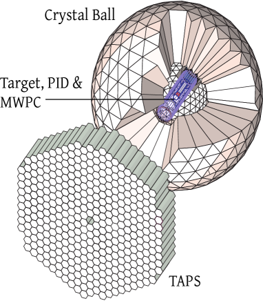
Figure 1: (Color online) A general sketch of the Crystal Ball, TAPS, and particle identification (PID) detectors.

The target was surrounded by a Particle IDentification (PID) detector PID used to distinguish between charged and neutral particles. It is made of 24 scintillator bars (50 cm long, 4 mm thick) arranged as a cylinder with a radius of 12 cm. A general sketch of the CB, TAPS, and PID is shown in Fig. 1. A multiwire proportional chamber, MWPC, also shown in this figure (which consists of two cylindrical MWPCs inside each other), was not installed during Run-I and was not used during Run-II as it could not operate in the high photon flux used in this experiment.

In Run-I, the energies of the incident photons were analyzed up to 1402 MeV by detecting the postbremsstrahlung electrons in the Glasgow tagged-photon spectrometer (Glasgow tagger) TAGGER ; TAGGER1 ; TAGGER2 , and up to 1448 MeV in Run-II. The uncertainty in the energy of the tagged photons is mainly determined by the segmentation of the tagger focal-plane detector in combination with the energy of the MAMI electron beam used in the experiments. Increasing the MAMI energy increases the energy range covered by the spectrometer and also has the corresponding effect on the uncertainty in $E_{\gamma}$. For both the MAMI energy settings of 1508 and 1557 MeV, this uncertainty was about $\pm 2$ MeV. More details on the tagger energy calibration and uncertainties in the energies can be found in Ref. EtaMassA2 .

The experimental trigger in Run-I required the total energy deposited in the CB to exceed $\sim$320 MeV and the number of so-called hardware clusters in the CB (multiplicity trigger) to be two or more. In the trigger, a hardware cluster in the CB was a block of 16 adjacent crystals in which at least one crystal had an energy deposit larger than 30 MeV. Depending on the data-taking period, events with a cluster multiplicity of two were prescaled with different rates. TAPS was not included in the multiplicity trigger for these experiments. In Run-II, the trigger on the total energy in the CB was increased to $\sim$340 MeV, and the multiplicity trigger required $\geq 3$ hardware clusters in the CB.

III Data handling

III.1 Selection of candidate events

To search for a signal from $\eta\to e^{+}e^{-}\gamma$ decays, candidates for the process $\gamma p\to e^{+}e^{-}\gamma p$ were extracted from events having three or four clusters reconstructed by a software analysis in the CB and TAPS together. The offline cluster algorithm was optimized for finding a group of adjacent crystals in which the energy was deposited by a single-photon e/m shower. This algorithm works well for $e^{+/-}$, which also produce e/m showers in the CB and TAPS, and for proton clusters. The software threshold for the cluster energy was chosen to be 12 MeV. For the $\gamma p\to e^{+}e^{-}\gamma p$ candidates, the three-cluster events were analyzed assuming that the final-state proton was not detected. The fraction of such $\eta\to e^{+}e^{-}\gamma$ decays was only about 20% from the total. Compared to the previous analysis of $\eta\to e^{+}e^{-}\gamma$, reported in Ref. eta_tff_a2_2014 , there were some improvements that resulted in a more reliable particle identification and in fewer sources of systematic uncertainties. Such improvements are discussed later in the text, including, for instance, the PID $dE/dx$ analysis for particle identification and adding the angular dependence of the virtual-photon decay in the Monte Carlo (MC) event generator for a more reliable acceptance determination.

To search for a signal from $\omega\to\pi^{0}e^{+}e^{-}$ decays, candidates for the process $\gamma p\to\pi^{0}e^{+}e^{-}p\to\gamma\gamma e^{+}e^{-}p$ were extracted from the analysis of events having five clusters (four from the photons and one from the proton) reconstructed in the CB and TAPS together. Four-cluster events, with only four photons detected, were neglected in the analysis because the proton information missing for such events in the analysis resulted in a much stronger background. In addition, as shown in Ref. a2_omegap_2015 , the fraction of $\gamma p\to\omega p\to\pi^{0}\gamma p$ events without the detected proton was quite small, varying from 2.7% at the reaction threshold to 7.6% at the highest energy of the present experiments.

The selection of candidate events and the reconstruction of the reaction kinematics was based on the kinematic-fit technique. Details of the kinematic-fit parametrization of the detector information and resolutions are given in Ref. slopemamic . Because the three-cluster sample, in which there are good $\gamma p\to\eta p\to e^{+}e^{-}\gamma p$ events without the outgoing proton detected, was mostly dominated by $\gamma p\to\pi^{0}p\to\gamma\gamma p$ and $\gamma p\to\eta p\to\gamma\gamma p$ events, the corresponding kinematic-fit hypotheses were tested first. Then all events for which the confidence level (CL) to be $\gamma p\to\pi^{0}p$ or $\gamma p\to\eta p$ was greater than $10^{-5}$ were discarded from further analysis. It was checked that such a preselection practically does not cause any losses of $\eta\to e^{+}e^{-}\gamma$ decays (which are $<1\%$), but rejects a significant background from two-photon final states. Because e/m showers from electrons and positrons are very similar to those of photons, the hypothesis $\gamma p\to 3\gamma p$ was tested to identify the $\gamma p\to e^{+}e^{-}\gamma p$ candidates. To identify $\omega\to\pi^{0}e^{+}e^{-}$ candidates, two hypotheses, $\gamma p\to 4\gamma p$ and $\gamma p\to\pi^{0}\gamma\gamma p\to 4\gamma p$, were tested. The events that satisfied these hypotheses with the CL greater than 1% were accepted for further analysis. The kinematic-fit output was used to reconstruct the kinematics of the outgoing particles. In this output, there was no separation between e/m showers caused by the outgoing photon, electron, or positron. Because the main purpose of the experiments was to measure the $\eta\to e^{+}e^{-}\gamma$ and $\omega\to\pi^{0}e^{+}e^{-}$ decay rates as a function of the invariant mass $m(e^{+}e^{-})$, the next step in the analysis was the separation of $e^{+}e^{-}$ pairs from final-state photons. This procedure was optimized by using a MC simulation of the processes $\gamma p\to\eta p\to e^{+}e^{-}\gamma p$ and $\gamma p\to\omega p\to\pi^{0}e^{+}e^{-}p\to\gamma\gamma e^{+}e^{-}p$.

III.2 Monte Carlo simulations

Those MC simulations were made to be as similar as possible to the real events to minimize the systematic uncertainties in the determination of experimental acceptances and to properly measure the energy dependence of the TFFs. To reproduce the experimental yield of $\eta$ and $\omega$ mesons and their angular distributions as a function of the incident-photon energy, both the $\gamma p\to\eta p$ and $\gamma p\to\omega p$ reactions were generated according to the numbers of the corresponding events and their angular distributions measured in the same experiment etamamic ; a2_omegap_2015 . The $\eta\to e^{+}e^{-}\gamma$ decays were generated according to Eq. (1), with the phase-space term removed and with $\Lambda^{-2}_{\eta}=1.95$ GeV^-2 from previous experiments NA60_2009 ; eta_tff_a2_2014 . The generation of the $\omega\to\pi^{0}e^{+}e^{-}$ decays were made in two steps. To reproduce the energy dependence of the $\omega$ decay width near the production threshold, the reaction $\gamma p\to\pi^{0}e^{+}e^{-}p$ was generated first according to phase space. Then, the invariant mass $m(\pi^{0}e^{+}e^{-})$ was folded with the Breit-Wigner (BW) function, with the parameters taken for the $\omega$ meson from the Review of Particle Physics (RPP) PDG . This approach allowed one to properly reproduce the folding of the BW shape with phase space. Next, the invariant mass $m(e^{+}e^{-})$ was folded to follow Eq. (3) with $\Lambda^{-2}_{\omega\pi^{0}}=2.24$ GeV^-2 NA60_2009 . The angular dependence of the virtual photon decaying into a lepton pair was generated according to Eq. (2), for both $\eta\to\gamma^{*}\gamma\to\ell^{+}\ell^{-}\gamma$ and $\omega\to\pi^{0}\gamma^{*}\to\pi^{0}\ell^{+}\ell^{-}$.

Possible background processes were also studied by using MC simulations. The reaction $\gamma p\to\eta p$ was simulated for several other decay modes of the $\eta$ meson to check if they could mimic a peak from the $\eta\to e^{+}e^{-}\gamma$ signal. Such MC simulations were made for the $\eta\to\gamma\gamma$, $\eta\to\pi^{0}\pi^{0}\pi^{0}$, $\eta\to\pi^{+}\pi^{-}\pi^{0}$, and $\eta\to\pi^{+}\pi^{-}\gamma$ decays. The yield and the production angular distributions of all $\gamma p\to\eta p$ simulations were generated in the same way as for the process $\gamma p\to\eta p\to e^{+}e^{-}\gamma p$. In contrast to the $\eta\to e^{+}e^{-}\gamma$ decay, all other $\eta$ decays were generated according to phase space. The major background under the peak from $\eta\to e^{+}e^{-}\gamma$ decays was found to be from the reaction $\gamma p\to\pi^{0}\pi^{0}p$. The MC simulation of this reaction was carried out in the same way as reported in Ref. p2pi0mamic . Although this background is smooth in the region of the $\eta$ mass and cannot mimic an $\eta\to e^{+}e^{-}\gamma$ peak, its MC simulation was used to optimize the signal-to-background ratio and to parametrize the background under the signal.

A similar study was also made for the $\omega\to\pi^{0}e^{+}e^{-}$ decay. The reaction $\gamma p\to\omega p$ was simulated for $\omega\to\pi^{0}\gamma$, with both the $\gamma\gamma$ and $\gamma e^{+}e^{-}$ decay modes of the $\pi^{0}$, and for $\omega\to\pi^{+}\pi^{-}\pi^{0}$ decays. The $\omega$ decay width was reproduced by folding $m(\pi^{0}\gamma)$ and $m(\pi^{+}\pi^{-}\pi^{0})$ in the processes $\gamma p\to\pi^{0}\gamma p$ and $\gamma p\to\pi^{+}\pi^{-}\pi^{0}p$ with the BW function having $\omega$ parameters from the RPP PDG . The Dalitz decay of the $\pi^{0}$ in $\omega\to\pi^{0}\gamma$ was generated according to its pure QED dependence. Additionally to the $\gamma p\to\pi^{0}\pi^{0}p$ background, the simulation of which was also needed for $\eta\to e^{+}e^{-}\gamma$, a study of the $\gamma p\to\pi^{0}\eta p$ background was made via its simulation.

For all reactions, the simulated events were propagated through a GEANT (version 3.21) simulation of the experimental setup. To reproduce the resolutions observed in the experimental data, the GEANT output (energy and timing) was subject to additional smearing, thus allowing both the simulated and experimental data to be analyzed in the same way. Matching the energy resolution between the experimental and MC events was achieved by adjusting the invariant-mass resolutions, the kinematic-fit stretch functions (or pulls), and probability distributions. Such an adjustment was based on the analysis of the same data sets for reactions having almost no background from other physical reactions (namely, $\gamma p\to\pi^{0}p$, $\gamma p\to\eta p\to\gamma\gamma p$, and $\gamma p\to\eta p\to 3\pi^{0}p$ slopemamic ). The simulated events were also tested to check whether they passed the trigger requirements.

III.3 Identifying $e^{+}e^{-}$ pairs and suppressing backgrounds

The PID detector was used to identify the final-state $e^{+}e^{-}$ pair (the detection efficiency for $e^{+/-}$ in the PID is close to 100%) in the events initially selected as $\gamma p\to 3\gamma p$ and $\gamma p\to 4\gamma p$ candidates. The $\gamma p\to\pi^{0}\gamma\gamma p\to 4\gamma p$ hypothesis was needed for selecting only $\gamma p\to\pi^{0}e^{+}e^{-}p$ candidates from the five-cluster events. Because, with respect to the LH₂ target, the PID provides a full coverage only for the CB crystals, events with at least three e/m showers in the CB were selected for further analysis, allowing one e/m shower to be detected in TAPS for $\gamma p\to\pi^{0}e^{+}e^{-}p$ candidates, and requiring the electron and positron to be detected in the CB. Requiring at least three e/m showers in the CB also made almost all selected events pass the trigger requirements on both the total energy and the multiplicity. The identification of $e^{+/-}$ in the CB was based on a correlation between the $\phi$ angles of fired PID elements with the angles of e/m showers in the calorimeter. The MC simulations of $\gamma p\to\eta p\to e^{+}e^{-}\gamma p$ and $\gamma p\to\omega p\to\pi^{0}e^{+}e^{-}p\to\gamma\gamma e^{+}e^{-}p$ were used to optimize this procedure, minimizing a probability of misidentification of $e^{+/-}$ with the final-state photons. This procedure is optimized with respect to how close the $\phi$ angle of an e/m shower in the CB should be to the corresponding angle of a fired PID element to be considered as $e^{+/-}$, and how far it should be to be considered as a photon. This decreases the efficiency in selecting true events for which the $\phi$ angle of the electron or the positron is close to the photon $\phi$ angle.

The analysis of the MC simulations of possible background reactions for $\eta\to e^{+}e^{-}\gamma$ revealed that only the process $\gamma p\to\eta p\to\gamma\gamma p$ could mimic $\eta\to e^{+}e^{-}\gamma$ events. This occurs mostly when one of the final-state photons converts into an $e^{+}e^{-}$ pair in the material between the production vertex and the NaI(Tl) surface. Because the opening angle between such electrons and positrons is typically very small, this background can be significantly suppressed by requiring that $e^{+}$ and $e^{-}$ were identified by different PID elements. However, such a requirement also decreases the detection efficiency for actual $\eta\to e^{+}e^{-}\gamma$ events, especially at low invariant masses $m(e^{+}e^{-})$. In further analysis of $\eta\to e^{+}e^{-}\gamma$ events, both the options, with larger and smaller background remaining from $\eta\to\gamma\gamma$, were tested.

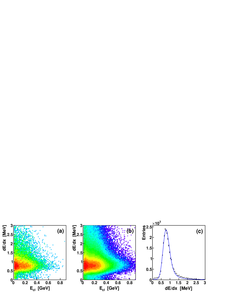
Figure 2: (Color online) Comparison of the $e^{+/-}$ $dE/dx$ of the PID for experimental $\eta\to e^{+}e^{-}\gamma$ decays and their MC simulation. The two-dimensional density distribution (with logarithmic scale along plot axis $z$) for the $e^{+/-}$ $dE/dx$ of the PID versus the energy of the corresponding clusters in the CB is shown in (a) for the experimental data and in (b) for the MC simulation. The $e^{+/-}$ $dE/dx$ distributions for the experimental data (crosses) and the MC simulation (blue solid line) are compared in (c).

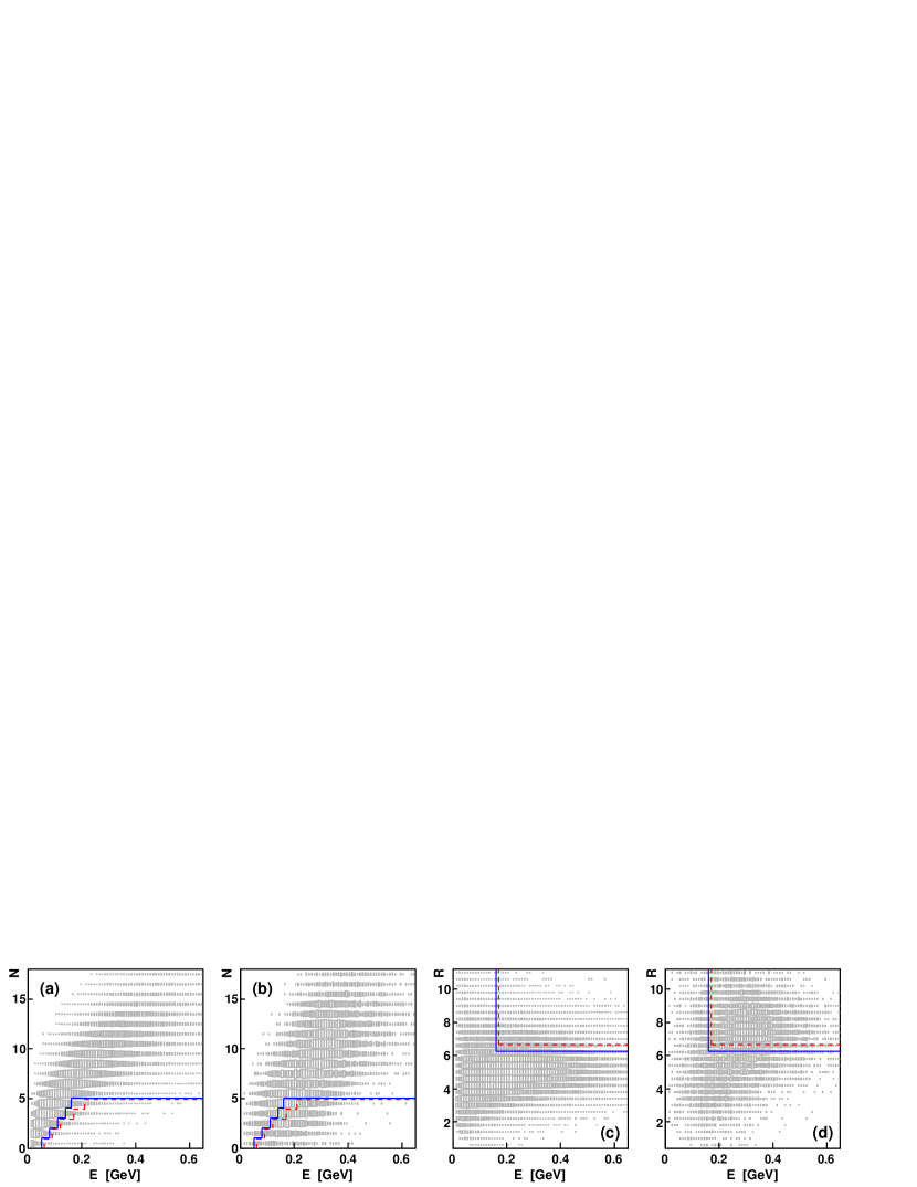
Figure 3: (Color online) (a), (c) Two-dimensional density distributions for events selected as the $\gamma p\to\pi^{0}e^{+}e^{-}p$ candidates obtained from the MC simulations of $\omega\to\pi^{0}e^{+}e^{-}$ decays and (b), (d) $\omega\to\pi^{0}\pi^{+}\pi^{-}$ decays causing background in the vicinity of the $\omega$ mass. Distributions (a) and (b) plot the number $N$ of crystals forming the two clusters ascribed to $e^{+/-}$ versus the cluster energies. Distributions (c) and (d) plot the effective radius $R$ of the two clusters ascribed to $e^{+/-}$ versus the cluster energies. The cuts tested for suppressing the $\omega\to\pi^{0}\pi^{+}\pi^{-}$ background are shown by red dashed lines for looser cuts and by blue solid lines for tighter cuts. The cuts on $N$ discard all events for which at least one of the $e^{+/-}$ clusters has an energy larger than the values shown by the cut lines. The cuts on effective radius discard all events for which at least one of the $e^{+/-}$ clusters has $R$ larger than the values shown by the cut lines.

Similarly, the process $\gamma p\to\omega p\to\pi^{0}\gamma p\to 3\gamma p$ can mimic $\omega\to\pi^{0}e^{+}e^{-}$ events via converting a final-state photon into an $e^{+}e^{-}$ pair. Another source of actual $\omega\to\gamma\gamma e^{+}e^{-}$ events comes from $\omega\to\pi^{0}\gamma$ decays with the Dalitz decay of $\pi^{0}$. Because of the QED dependence of this decay, it dominates at low masses $m(e^{+}e^{-})$ and can be suppressed by requiring that $e^{+}$ and $e^{-}$ were identified by different PID elements. Further reduction of this background can be achieved by requiring the two final-state photons to be from the $\pi^{0}$ decay.

Other background sources that should be significantly suppressed in the analysis of $\omega\to\pi^{0}e^{+}e^{-}$ events are the processes $\gamma p\to\pi^{0}\pi^{0}p$ and $\gamma p\to\pi^{0}\eta p$, with the $\eta$ meson decaying into two photons or into $e^{+}e^{-}\gamma$. In the case of the two-photon decay, both the photons can convert before or inside the PID, mimicking an $e^{+}e^{-}$ pair. In the case of the $e^{+}e^{-}\gamma$ decay, $e^{+}e^{-}$ pairs with very low invariant masses often hit the same PID element and are reconstructed as one cluster in the CB. If the photon from the same decay converts before or inside the PID, such an event could be identified as a $\pi^{0}e^{+}e^{-}$ final state. Similarly, the process $\gamma p\to\pi^{0}\pi^{0}p$ can mimic $\gamma p\to\pi^{0}e^{+}e^{-}p$ events. Without suppressing background from $\gamma p\to\pi^{0}\pi^{0}p$ and $\gamma p\to\pi^{0}\eta p$, the signal from $\omega\to\pi^{0}e^{+}e^{-}$ would be comparable with the statistical fluctuations of the background events, preventing the measurement of the TFF at $m(e^{+}e^{-})$ close to the $\pi^{0}$ and $\eta$ masses, with the $\eta$-mass region being especially important for the $\omega\pi^{0}$ TFF.

The suppression of background from $\gamma p\to\pi^{0}\pi^{0}p$ and $\gamma p\to\pi^{0}\eta p$ was based on the analysis of energy losses, $dE/dx$, in the PID elements. According to the MC simulations of these backgrounds, many photons produce energy losses that are significantly smaller than $dE/dx$ from a single $e^{+/-}$, and the $e^{+}e^{-}$ pairs reconstructed as one cluster in the CB result in a double-magnitude PID signal, compared to a single $e^{+/-}$. To reflect the actual differential energy deposit $dE/dx$ in the PID, the energy signal from each element, ascribed to either $e^{+}$ or $e^{-}$, was multiplied by the sine of the polar angle of the corresponding particle, the magnitude of which is taken from the kinematic-fit output. All PID elements were calibrated so that the $e^{+/-}$ peak position matched the corresponding peak in the MC simulation. To reproduce the actual energy resolution of the PID with the MC simulation, the GEANT output for PID energies was subject to additional smearing, allowing the $e^{+/-}$ selection with $dE/dx$ cuts to be very similar for the experimental data and MC. The PID energy resolution in the MC simulations was adjusted to match the experimental $dE/dx$ spectra for the $e^{+/-}$ particles produced in $\eta\to e^{+}e^{-}\gamma$ decays with $m(e^{+}e^{-})$ below the $\pi^{0}$ mass, the range in which these decays can be selected with very small background, especially if the final-state proton is detected (this will be illustrated further in the text). The same sample was used to check possible systematic uncertainties due to losses of good events while applying $dE/dx$ cuts to suppress background from $\gamma p\to\pi^{0}\pi^{0}p$ and $\gamma p\to\pi^{0}\eta p$.

The experimental $dE/dx$ resolution of the PID for $e^{+/-}$ and the comparison of it with the MC simulation is illustrated in Fig. 2. Figures 2(a) and (b) compare the experimental and MC-simulation plots of the $e^{+/-}$ $dE/dx$ of the PID versus the energy of the corresponding clusters in the CB. As seen, there is no $dE/dx$ dependence of $e^{+/-}$ on their energy in the CB, and applying cuts just on a $dE/dx$ value is sufficient for suppressing background from $\gamma p\to\pi^{0}\pi^{0}p$ and $\gamma p\to\pi^{0}\eta p$. The comparison of the experimental $e^{+/-}$ $dE/dx$ distributions with the MC simulation is depicted in Fig. 2(c). A small difference in the tails of the $e^{+/-}$ peak can be explained by some background remaining in the experimental spectrum. Typical PID cuts, which were tested, varied from requiring $dE/dx<2.7$ MeV to $dE/dx<1.2$ MeV to suppress background events, showing no systematic effects in the final results.

The $\omega\to\pi^{0}\pi^{+}\pi^{-}$ decay can mimic the $\pi^{0}e^{+}e^{-}$ final state when both charged pions deposit their total energy due to nuclear interactions in the CB. The probability of such events is quite low, but the branching ratio for $\omega\to\pi^{0}\pi^{+}\pi^{-}$ is a factor $\sim 2\times 10^{3}$ greater than for $\omega\to\pi^{0}e^{+}e^{-}$. The suppression of the $\omega\to\pi^{0}\pi^{+}\pi^{-}$ background to a level negligible for $\omega\to\pi^{0}e^{+}e^{-}$ events typically requires a combination of a few selection criteria. The energy resolution of the PID is not sufficient to efficiently separate $\pi^{+/-}$ from $e^{+/-}$ by the $dE/dx$ method. Most of the background events from $\omega\to\pi^{0}\pi^{+}\pi^{-}$ decays have a low probability for $\gamma p\to\pi^{0}\gamma\gamma p\to 4\gamma p$, and the position of the event vertex along the beam direction ($z$ axis), reconstructed by the kinematic fit, is strongly shifted in the downstream direction. Such a shift in $z$ is caused by an attempt by the kinematic fit to compensate for an imbalance in energy conservation by changing significantly the polar angles of the outgoing particles, which is only possible by moving the event vertex along the beam direction. Accordingly, applying cuts on the kinematic-fit CL and the vertex coordinate $z$ mostly rejects $\omega\to\pi^{0}\pi^{+}\pi^{-}$ events with cluster energies of $\pi^{+/-}$ below their total energies. Typically, such events are reconstructed by the kinematic fit with invariant masses $m(\pi^{0}e^{+}e^{-})$ below the mass of the $\omega$ meson. Further suppression of the $\omega\to\pi^{0}\pi^{+}\pi^{-}$ background events remaining in the vicinity of the $\omega$ mass can be achieved by using differences in features of e/m and nuclear-interaction showers in the CB. As observed from MC simulations of $\omega\to\pi^{0}e^{+}e^{-}$ and $\omega\to\pi^{0}\pi^{+}\pi^{-}$ decays, nuclear-interaction showers at lower energies typically have a smaller multiplicity of the crystals forming a cluster. At higher energies, nuclear-interaction showers from $\pi^{+/-}$ typically spread more widely than e/m showers. Such a spread can be evaluated via the cluster effective radius. For the CB, the effective radius $R$ of a cluster containing $k$ crystals with energy $E_{i}$ deposited in crystal $i$ can be defined as

$$R=(\sum^{k}_{i}{E_{i}(\Delta r_{i})^{2}}/\sum^{k}_{i}{E_{i}})^{1/2}~{},$$ (5)

where $\Delta r_{i}$ is the opening angle (in degrees) between the cluster direction (as determined by the cluster algorithm) and the crystal-axis direction. The multiplicity $N$ of the crystals forming a cluster ascribed to $e^{+/-}$ is shown as a function of the cluster energy in Figs. 3(a) and (b), respectively for the MC simulations of $\omega\to\pi^{0}e^{+}e^{-}$ decays and $\omega\to\pi^{0}\pi^{+}\pi^{-}$ decays causing background in the vicinity of the $\omega$ mass. Similar distributions for the effective radius $R$ of clusters ascribed to $e^{+/-}$ are shown in Figs. 3(c) and (d). The cuts tested for suppressing the $\omega\to\pi^{0}\pi^{+}\pi^{-}$ background are depicted by red dashed lines for looser cuts and by blue solid lines for tighter cuts. The cuts on $N$ discard all events for which at least one of the clusters ascribed to $e^{+/-}$ has an energy larger than the value shown by the corresponding cut lines. The cuts on effective radius discard all events for which at least one of $e^{+/-}$ clusters has $R$ larger than the values shown by the cut lines. These cuts were optimized to significantly suppress the $\omega\to\pi^{0}\pi^{+}\pi^{-}$ background with minimal losses of $\omega\to\pi^{0}e^{+}e^{-}$ decays. To make sure that these cuts do not cause systematic uncertainties in the $\omega\to\pi^{0}e^{+}e^{-}$ results, the same cuts were tested in the analysis of the $\eta\to e^{+}e^{-}\gamma$ decay, which has much better statistics and less background.

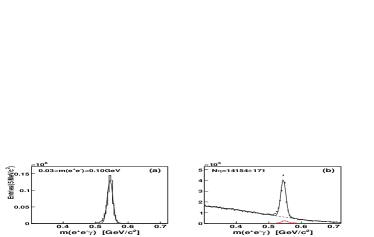
Figure 4: (Color online) $m(e^{+}e^{-}\gamma)$ invariant-mass distributions obtained for the $m(e^{+}e^{-})$ range from 30 to 100 MeV/$c^{2}$ with $\gamma p\to e^{+}e^{-}\gamma p$ candidates initially selected with the kinematic fit and allowing both $e^{+}$ and $e^{-}$ to be identified with the same PID element: (a) MC simulation of $\gamma p\to\eta p\to e^{+}e^{-}\gamma p$ fitted with a Gaussian; (b) experimental events (Run-I) after subtracting the random background and the remaining background from $\gamma p\to\eta p\to\gamma\gamma p$. The distribution for the $\eta\to\gamma\gamma$ background, shown by a red solid line, is normalized to the number of subtracted events. The experimental distribution is fitted with the sum of a Gaussian for the $\eta\to e^{+}e^{-}\gamma$ peak and a polynomial of order four for the background. The total fit is depicted by a solid line, and the dashed line shows the background under the peak.

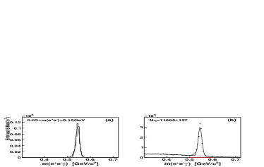
Figure 5: (Color online) Same as Fig. 4, but requiring both $e^{+}$ and $e^{-}$ to be identified by different PID elements.

Figure 6: (Color online) Same as Fig. 5, but after applying the $dE/dx$ PID cut selecting only events with the elements having an energy deposit corresponding to a single $e^{+/-}$, and requiring the final-state proton to be detected.

In addition to the background contributions from other physical reactions, there are two more background sources. The first source comes from interactions of incident photons in the windows of the target cell. The subtraction of this background from experimental spectra is typically based on the analysis of data samples that were taken with an empty target. In the present analysis, the empty-target background was small and did not feature any visible $\eta$ peak in its $m(e^{+}e^{-}\gamma)$ spectra for the $\gamma p\to e^{+}e^{-}\gamma p$ candidates nor any $\omega$ peak in its $m(\pi^{0}e^{+}e^{-})$ spectra for the $\gamma p\to\pi^{0}e^{+}e^{-}p$ candidates. Another background was caused by random coincidences of the tagger counts with the experimental trigger; its subtraction was carried out by using event samples for which all coincidences were random (see Refs. slopemamic ; etamamic for more details).

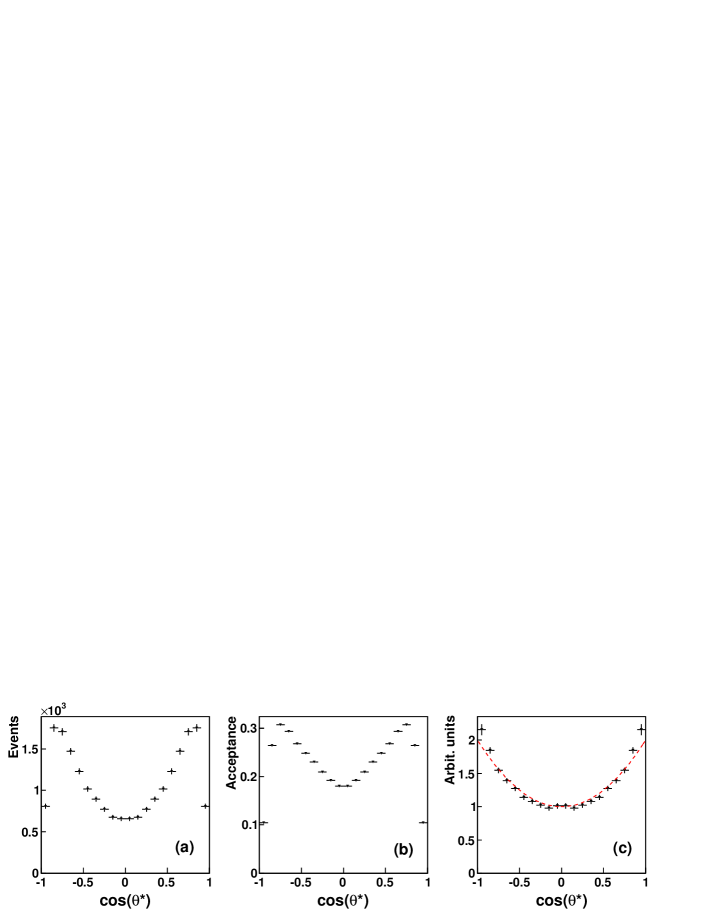
Figure 7: (Color online) The $\eta\to\gamma\gamma^{*}\to\gamma e^{+}e^{-}$ angular dependence (in the $\eta$ rest frame) of the virtual photon decaying into a lepton pair, with $\theta^{*}$ being the angle between the direction of one of the leptons in the virtual-photon (or the dilepton) rest frame and the direction of the dilepton system (which is opposite to the $\gamma$ direction): (a) experimental events from the $\eta\to\gamma e^{+}e^{-}$ peak; (b) angular acceptance based on the MC simulation; (c) the experimental spectrum corrected for the acceptance and normalized for comparing to the $1+\cos^{2}\theta^{*}$ dependence (shown by a red dashed line). Because $e^{+}$ and $e^{-}$ cannot be separated in the present experiment, the angles of both leptons were used, resulting in a symmetric shape with respect to $\cos\theta^{*}=0.$

III.4 Measuring $\eta\to e^{+}e^{-}\gamma$ and $\omega\to\pi^{0}e^{+}e^{-}$ and checking systematic uncertainties

To measure the $\eta\to e^{+}e^{-}\gamma$ and $\omega\to\pi^{0}e^{+}e^{-}$ yield as a function of the invariant mass $m(e^{+}e^{-})$, the corresponding candidate events were divided into several $m(e^{+}e^{-})$ bins. The width of the $m(e^{+}e^{-})$ bins was chosen to be narrower at low masses, where the QED dependence results in much higher statistics of Dalitz decays, and to be wider at large $m(e^{+}e^{-})$ masses with fewer Dalitz decays. Events with $m(e^{+}e^{-})<30$ MeV/$c^{2}$ were not analyzed at all, because e/m showers from those $e^{+}$ and $e^{-}$ start to overlap too much in the CB. The number of $\eta\to e^{+}e^{-}\gamma$ and $\omega\to\pi^{0}e^{+}e^{-}$ decays in every $m(e^{+}e^{-})$ bin was determined by fitting the experimental $m(e^{+}e^{-}\gamma)$ and $m(\pi^{0}e^{+}e^{-})$ spectra with the $\eta$ and $\omega$ peaks rising above a smooth background. Possible systematic uncertainties in the results owing to various cuts on the kinematic-fit CL, the vertex coordinate $z$, $dE/dx$ of PID, the multiplicity $N$ of the crystals forming $e^{+/-}$ clusters, and their effective radius $R$ were studied by using enlarged $m(e^{+}e^{-})$ bins, allowing greater statistics for such a study. The events with $e^{+}$ and $e^{-}$ detected with the same PID element were analyzed only for the $\eta\to e^{+}e^{-}\gamma$ decay. For the $\omega\to\pi^{0}e^{+}e^{-}$ decay, such an option resulted in too much background in the region of the $\omega$ peak.

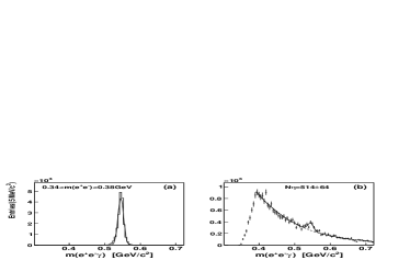
Figure 8: Same as Fig. 4, but for $m(e^{+}e^{-})=(360\pm 20)$ MeV/$c^{2}$. The $\eta\to\gamma\gamma$ background is not shown in (b) because it is negligibly small.

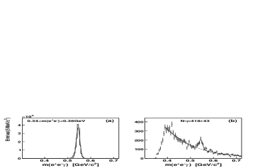
Figure 9: Same as Fig. 8, but after applying the softer cuts on $N$ and $R$ (depicted by red dashed lines in Fig. 3).

The fitting procedure for $\eta\to e^{+}e^{-}\gamma$ and the impact of selection criteria on the background is illustrated in Figs. 4–6 and Figs. 8–10. Figure 4 shows all $\gamma p\to e^{+}e^{-}\gamma p$ candidates in the $m(e^{+}e^{-})$ range from 30 to 100 MeV/$c^{2}$. These were initially selected with the kinematic-fit CL only, also allowing both $e^{+}$ and $e^{-}$ to be identified with the same PID element. Figure 4(a) depicts the $m(e^{+}e^{-}\gamma)$ invariant-mass distribution for the MC simulation of $\gamma p\to\eta p\to e^{+}e^{-}\gamma p$ fitted with a Gaussian. The experimental distribution after subtracting both the random background and the background remaining from $\gamma p\to\eta p\to\gamma\gamma p$ is shown by crosses in Fig. 4(b). The distribution for the $\eta\to\gamma\gamma$ background is normalized to the number of subtracted events and is shown in the same figure by a red solid line. The subtraction normalization was based on the number of events generated for $\gamma p\to\eta p\to\gamma\gamma p$ and the number of $\gamma p\to\eta p$ events produced in the same experiment. The experimental distribution was fitted with the sum of a Gaussian for the $\eta\to e^{+}e^{-}\gamma$ peak and a polynomial of order four for the background. In this fit, the centroid and width of the Gaussian were fixed to the values obtained from the previous Gaussian fit to the $\gamma p\to\eta p\to e^{+}e^{-}\gamma p$ MC simulation, which is shown in Fig. 4(a). As seen, the Gaussian parameters obtained from fitting to the MC simulation suit the experimental peak well. This confirms the agreement of the experimental data and the MC simulation in the energy calibration of the calorimeters and their resolution. The order of the polynomial was chosen to be sufficient for a reasonable description of the background distribution in the range of fitting.

The number of $\eta\to e^{+}e^{-}\gamma$ decays in the experimental $m(e^{+}e^{-}\gamma)$ spectra was determined from the area under the Gaussian. For consistency, the $\gamma p\to\eta p\to e^{+}e^{-}\gamma p$ detection efficiency in each $m(e^{+}e^{-})$ bin was obtained in the same way, i.e., based on the $m(e^{+}e^{-}\gamma)$ spectrum for the MC simulation fitted with a Gaussian, instead of using the number of entries in this spectrum. For the selection criteria and the $m(e^{+}e^{-})$ range used to obtain the spectra shown in Fig. 4, the averaged detection efficiency determined for $\gamma p\to\eta p\to e^{+}e^{-}\gamma p$ in this manner is 33.1%.

Figure 5 illustrates the effect of requiring both $e^{+}$ and $e^{-}$ to be identified by different PID elements. As seen, compared to Fig. 4(b), the $\eta\to\gamma\gamma$ background becomes very small. The signal-to-background ratio improves significantly as well, whereas the $\gamma p\to\eta p\to e^{+}e^{-}\gamma p$ detection efficiency decreases to 25.8%. The results for the $\eta\to e^{+}e^{-}\gamma$ yield obtained with and without adding events with $e^{+}$ and $e^{-}$ identified by the same PID element showed good agreement within the fit uncertainties, confirming the reliability of the $\eta\to\gamma\gamma$ background subtraction.

The almost full elimination of the background contributions under the $\eta\to e^{+}e^{-}\gamma$ peak in this $m(e^{+}e^{-})$ range can be obtained by applying the $dE/dx$ PID cut selecting only events with the elements having a deposit corresponding to a single $e^{+/-}$, and also requiring the final-state proton to be detected. The spectra obtained with such cuts are shown in Fig. 6. Although the $\gamma p\to\eta p\to e^{+}e^{-}\gamma p$ detection efficiency decreases to 22.3%, the smallness of the background under the $\eta\to e^{+}e^{-}\gamma$ peak makes it possible to measure the $\eta\to\gamma\gamma^{*}\to\gamma e^{+}e^{-}$ angular dependence of the virtual photon decaying into a lepton pair and to compare it with Eq. (2).

Figure 10: Same as Fig. 8, but after applying the tighter cuts on $N$ and $R$ (depicted by blue solid lines in Fig. 3).

The experimental results for such an angular dependence are illustrated in Fig. 7. Figure 7(a) shows the experimental $\cos\theta^{*}$ distribution obtained for the events in the $\eta\to e^{+}e^{-}\gamma$ peak from Fig. 6(b). The corresponding angular acceptance determined from the MC simulation is depicted in Fig. 7(b). The experimental $\cos\theta^{*}$ distribution corrected for the acceptance is depicted in Fig. 7(c), showing reasonable agreement with the expected $1+\cos^{2}\theta^{*}$ dependence. Because $e^{+}$ and $e^{-}$ cannot be separated in the present experiment, the angles of both leptons were used to measure the dilepton decay dependence, which resulted in a symmetric shape with respect to $\cos\theta^{*}=0.$

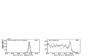
Figure 11: (Color online) $m(\pi^{0}e^{+}e^{-})$ invariant-mass distributions obtained for the $m(e^{+}e^{-})$ range from 30 to 100 MeV/$c^{2}$ with $\gamma p\to\pi^{0}e^{+}e^{-}p$ candidates initially selected with the kinematic fit (a) MC simulation of $\gamma p\to\omega p\to\pi^{0}e^{+}e^{-}p$ fitted with a Gaussian; (b) experimental events (Run-I) after subtracting the random background and the remaining background from $\omega\to\pi^{0}\gamma$ decays (with both the $\pi^{0}\to\gamma\gamma$ and $\pi^{0}\to e^{+}e^{-}\gamma$ decay modes). The distribution for the $\omega\to\pi^{0}\gamma$ background, shown by a red solid line, is normalized to the number of subtracted events. The experimental distribution is fitted with the sum of a Gaussian for the $\omega\to\pi^{0}e^{+}e^{-}$ peak and a polynomial of order five for the background. The total fit is depicted by a solid line, and the dashed line shows the background under the peak.

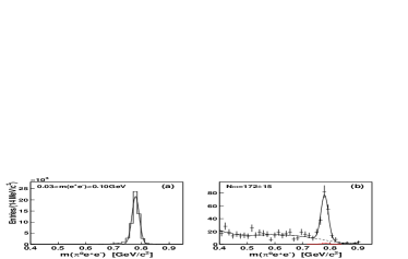
Figure 12: (Color online) Same as Fig. 11, but after applying the softer cuts on $N$ and $R$ (depicted by red dashed lines in Fig. 3) and the $dE/dx$ cut rejecting events with twice the magnitude of a signal from a single $e^{+/-}$ in one PID element.

At higher $m(e^{+}e^{-})$ masses, in addition to $\gamma p\to\pi^{0}\pi^{0}p$ events, there is background from $\eta\to\pi^{+}\pi^{-}\gamma$ and $\eta\to\pi^{+}\pi^{-}\pi^{0}$ decays. These decays do not mimic the $\eta\to e^{+}e^{-}\gamma$ peak, but, without suppression of the $\pi^{+/-}$ background, the signal becomes comparable with the statistical fluctuations of the background events. The suppression of this background with the cuts on the multiplicity $N$ of the crystals forming $e^{+/-}$ clusters and their effective radius $R$ is illustrated in Figs. 8–10.

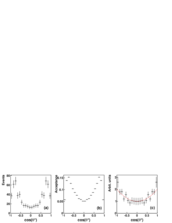
Figure 13: (Color online) The $\omega\to\pi^{0}\gamma^{*}\to\pi^{0}e^{+}e^{-}$ angular dependence (in the $\omega$ rest frame) of the virtual photon decaying into a lepton pair, with $\theta^{*}$ being the angle between the direction of one of the leptons in the virtual-photon (or the dilepton) rest frame and the direction of the dilepton system (which is opposite to the $\pi^{0}$ direction): (a) experimental events from the $\omega\to\pi^{0}e^{+}e^{-}$ peak; (b) angular acceptance based on the MC simulation; (c) the experimental spectrum corrected for the acceptance and normalized for comparing to the $1+\cos^{2}\theta^{*}$ dependence (shown by a red dashed line). Because $e^{+}$ and $e^{-}$ cannot be separated in the present experiment, the angles of both leptons were used, resulting in a symmetric shape with respect to $\cos\theta^{*}=0.$

Figure 8 shows $\gamma p\to e^{+}e^{-}\gamma p$ candidates selected with the kinematic-fit CL in the $m(e^{+}e^{-})$ region, where the magnitude of the $\eta\to e^{+}e^{-}\gamma$ peak is still sufficient to see it above a large background. The result of applying the softer cuts on $N$ and $R$ (depicted by red dashed lines in Fig. 3) is demonstrated in Fig. 9, showing a significant improvement in the signal-to-background ratio. The further improvement with the tighter cuts on $N$ and $R$ (depicted by blue solid lines in Fig. 3) is demonstrated in Fig. 10. The fits with the suppressed background in this $m(e^{+}e^{-})$ range are more reliable, even if the $\gamma p\to\eta p\to e^{+}e^{-}\gamma p$ detection efficiency decreases from 33.4% to 27.8% after applying the softer cuts, and to 24.0% after applying the tighter cuts. It was checked that the results for the $\eta\to e^{+}e^{-}\gamma$ yield obtained with and without cuts on $N$ and $R$ were in good agreement within the fit uncertainties, confirming the reliability of the method based on the difference in the features of $e^{+/-}$ and $\pi^{+/-}$ clusters. Note that the $\eta\to\gamma\gamma$ background is negligibly small in this range of $m(e^{+}e^{-})$ masses, even with both $e^{+}$ and $e^{-}$ being identified by the same PID elements.

Because the $\omega\to\pi^{0}e^{+}e^{-}$ decays were analyzed in the same data sets and by using the same cuts, the systematic uncertainties caused by these cuts should be the same as for $\eta\to e^{+}e^{-}\gamma$. Additional tests were made for $m(e^{+}e^{-})$ ranges with less background and wide $m(e^{+}e^{-})$ bins, giving smaller statistical uncertainties in the results. The fitting procedure for $\omega\to\pi^{0}e^{+}e^{-}$ (which is very similar to $\eta\to e^{+}e^{-}\gamma$) and some of the tests, including the $\omega\to\pi^{0}\gamma^{*}\to\pi^{0}e^{+}e^{-}$ angular dependence of the virtual photon decaying into a lepton pair, are illustrated in Figs. 11–15.

Figure 11 shows $\gamma p\to\pi^{0}e^{+}e^{-}p$ candidates selected only with the kinematic-fit CL, for the $m(e^{+}e^{-})$ region below the $\pi^{0}$ mass, avoiding very large background from $\gamma p\to\pi^{0}\pi^{0}p$. Figure 11(a) depicts the $m(\pi^{0}e^{+}e^{-})$ invariant-mass distribution for the MC simulation of $\gamma p\to\omega p\to\pi^{0}e^{+}e^{-}p$ fitted with a Gaussian. The choice of the normal distribution for fitting the $\omega$ peak is motivated by the facts that the BW shape of the $\omega$ signal is severely cut by phase space near threshold and the $m(\pi^{0}e^{+}e^{-})$ resolution strongly dominates the $\omega$-meson width ($\Gamma=8.49$ MeV PDG ). A similar approach was successfully used for fitting the $\omega\to\pi^{0}\gamma$ peak above background while measuring $\omega$ photoproduction with the same data set a2_omegap_2015 . The experimental distribution after subtracting both the random background and the background remaining from $\omega\to\pi^{0}\gamma$ decays (with both the $\pi^{0}\to\gamma\gamma$ and $\pi^{0}\to e^{+}e^{-}\gamma$ decay modes) is shown by crosses in Fig. 11(b). The distribution for the $\omega\to\pi^{0}\gamma$ background is normalized to the number of subtracted events and is shown in the same figure by a red solid line. The subtraction normalization was based on the number of events generated for $\gamma p\to\omega p\to\pi^{0}\gamma p$ and the number of $\gamma p\to\omega p$ events produced in the experiment. The experimental distribution was fitted with the sum of a Gaussian for the $\omega\to\pi^{0}e^{+}e^{-}$ peak and a polynomial of order five for the background. In this fit, the centroid and width of the Gaussian were fixed to the values obtained from the previous Gaussian fit to the $\gamma p\to\omega p\to\pi^{0}e^{+}e^{-}p$ MC simulation, which is shown in Fig. 11(a). Similar to $\eta\to e^{+}e^{-}\gamma$, the number of $\omega\to\pi^{0}e^{+}e^{-}$ decays in the MC and experimental $m(\pi^{0}e^{+}e^{-})$ spectra was determined from the area under the Gaussian. For the selection criteria used to obtain the spectra in Fig. 11 and the given $m(e^{+}e^{-})$ range, the averaged detection efficiency determined for $\omega\to\pi^{0}e^{+}e^{-}$ is 14.5%.

Figure 12 illustrates the impact of the PID $dE/dx$ cut and the softer cuts on $N$ and $R$ on suppressing background under the $\omega$ peak. As seen, compared to Fig. 11(b), the quantity of background events becomes smaller by a factor of 5 (resulting in a more reliable fit to the signal peak), whereas the detection efficiency for $\omega\to\pi^{0}e^{+}e^{-}$ decreases to 9.1%.

Although the level of the background remaining under the $\omega\to\pi^{0}e^{+}e^{-}$ peak is not negligibly small, it is still possible to check the $\omega\to\pi^{0}\gamma^{*}\to\pi^{0}e^{+}e^{-}$ angular dependence of the virtual photon decaying into a lepton pair, compared to Eq. (2). The experimental results for such an angular dependence are illustrated in Fig. 13.

Figure 13(a) shows the experimental $\cos\theta^{*}$ distribution obtained for the events in the $\omega\to\pi^{0}e^{+}e^{-}$ peak from Fig. 12(b). The corresponding angular acceptance determined from the MC simulation is depicted in Fig. 13(b). The experimental $\cos\theta^{*}$ distribution corrected for the acceptance is depicted in Fig. 13(c), showing, for the very limited statistics and the remaining background, reasonable agreement with the expected $1+\cos^{2}\theta^{*}$ dependence.

Figure 14: Same as Fig. 11, but for the $m(e^{+}e^{-})$ range from 150 to 400 MeV/$c^{2}$ and the tighter cuts on $N$ and $R$ (depicted by blue solid lines in Fig. 3). The $\omega\to\pi^{0}\gamma$ background is not shown in (b) because it is negligibly small.

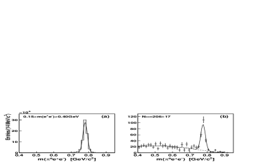
Figure 15: Same as Fig. 14, but after applying the $dE/dx$ cut rejecting events with twice the magnitude of a signal from a single $e^{+/-}$ in one PID element.

Figures 14 and 15 illustrate fits for the $m(e^{+}e^{-})$ region above the $\pi^{0}$ mass, with $\gamma p\to\pi^{0}e^{+}e^{-}p$ candidates selected after the tighter cuts on $N$ and $R$ (better suppressing the $\omega\to\pi^{0}\pi^{+}\pi^{-}$ background), and without and with $dE/dx$ PID cuts. As seen from these figures, the quantity of background events in the vicinity of the $\omega$ peak becomes smaller by a factor of more than 4 after applying the $dE/dx$ PID cut, whereas the detection efficiency, averaged in this $m(e^{+}e^{-})$ range, decreases from 18.9% to 15.1%. The $\omega\to\pi^{0}\gamma$ background is negligibly small in this range of $m(e^{+}e^{-})$ masses, and it is not shown in these figures. The fits made without and with $dE/dx$ PID cuts showed good agreement within the fit uncertainties, confirming the reliability of tests made with the $\eta\to e^{+}e^{-}\gamma$ decay.

To measure the $\eta\to e^{+}e^{-}\gamma$ and $\omega\to\pi^{0}e^{+}e^{-}$ yields as a function of the invariant mass $m(e^{+}e^{-})$, the corresponding candidate events were divided into several $m(e^{+}e^{-})$ bins, separately for Run-I and Run-II. The available statistics and the level of background for $\eta\to e^{+}e^{-}\gamma$ decays enabled division of the $m(e^{+}e^{-})$ range from 30 to 490 MeV/$c^{2}$ into 34 bins, with bin widths increasing from 10 MeV/$c^{2}$ at the lowest masses to 30 MeV/$c^{2}$ at the highest masses. To measure the $\omega\to\pi^{0}e^{+}e^{-}$ decay, the $m(e^{+}e^{-})$ range from 30 to 630 MeV/$c^{2}$ was divided into 14 bins, with bin widths increasing from 20 MeV/$c^{2}$ at the lowest masses to 60 MeV/$c^{2}$ at the highest masses. The size and width of the $m(e^{+}e^{-})$ bins for Run-I and Run-II were identical, which later allowed the results from both runs to be combined. The fitting procedure was the same as those used to check the systematic uncertainties caused by various selection criteria.

IV Results and discussion

IV.1 TFF results and their uncertainties

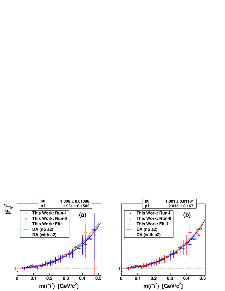
Figure 16: (Color online) Comparison of the $|F_{\eta}(m_{\ell^{+}\ell^{-}})|^{2}$ results obtained individually from the analyses of Run-I (blue filled triangles) and Run-II (red open circles) with each other and with the two solutions for the DA calculations by the Jülich group Xiao_2015 ; Hanhart . The solution without including the $a_{2}$-meson contribution is shown by a red dotted line with an error band, and the solution involving the $a_{2}$ contribution is shown by a blue dashed line. The pole-approximation fits (black solid lines) to the results of Run-I and Run-II are depicted in panels (a) and (b), respectively. The fit parameter $p0$ reflects the general normalization of the data points, and $p1$ is the slope parameter $\Lambda^{-2}$ [GeV^-2]. For a better comparison of the magnitudes of total uncertainties from the two data sets, the error bars of Run-I are plotted in (a) on the top of the error bars of Run-II, and the other way around in (b).

The total number of $\eta\to e^{+}e^{-}\gamma$ and $\omega\to\pi^{0}e^{+}e^{-}$ decays initially produced in each $m(e^{+}e^{-})$ bin was obtained by correcting the number of decays observed in each bin with the corresponding detection efficiency. Values of $d\Gamma(\eta\to e^{+}e^{-}\gamma)/dm(e^{+}e^{-})$ and $d\Gamma(\omega\to\pi^{0}e^{+}e^{-})/dm(e^{+}e^{-})$ for every fit were obtained from those initial numbers of decays by taking into account the full decay width of $\eta$ and $\omega$ PDG , the total number of $\eta$ and $\omega$ mesons produced in the same data sets etamamic ; a2_omegap_2015 , and the width of the corresponding $m(e^{+}e^{-})$ bin. The uncertainty in an individual $d\Gamma/dm(e^{+}e^{-})$ value from a particular fit was based on the uncertainty in the number of decays determined by this fit (i.e., the uncertainty in the area under the Gaussian). The systematic uncertainties in the $d\Gamma/dm(e^{+}e^{-})$ value were estimated for each individual $m(e^{+}e^{-})$ bin by repeating its fitting procedure several times after refilling the $m(e^{+}e^{-}\gamma)$ spectra with different combinations of selection criteria, which were used to improve the signal-to-background ratio, or after slight changes in the parametrization of the background under the signal peak. The changes in selection criteria included cuts on the kinematic-fit CL (such as 2%, 5%, 10%, 15%, and 20%), different cuts on PID $dE/dx$, $N$, $R$, and $z$. As in Ref. eta_tff_a2_2014 , the $\eta\to e^{+}e^{-}\gamma$ results were also checked for excluding three-cluster events (no final-state proton detected) from the analysis. The requirement of making several fits for each $m(e^{+}e^{-})$ bin provided a check on the stability of the $d\Gamma/dm(e^{+}e^{-})$ results. The average of the results of all fits made for one bin was then used to obtain final $d\Gamma/dm$ values that were more reliable than the results based on just one so-called best fit, which was made with a combination of selection criteria, giving the optimal number of events in the signal peak with respect to the background level under it. Typically, such a best fit gives the largest ratio between the corresponding $d\Gamma/dm$ value and its uncertainty.

Table 1: Results of this work for the $\eta$ TFF, $|F_{\eta}|^{2}$, as a function of the invariant mass $m(e^{+}e^{-})$.

$m(e^{+}e^{-})$ [MeV/$c^{2}$]	$35\pm 5$	$45\pm 5$	$55\pm 5$	$65\pm 5$	$75\pm 5$	$85\pm 5$	$95\pm 5$
$|F_{\eta}|^{2}$	$1.006\pm 0.024$	$0.999\pm 0.022$	$1.013\pm 0.021$	$1.037\pm 0.024$	$1.032\pm 0.024$	$1.057\pm 0.031$	$1.070\pm 0.030$
$m(e^{+}e^{-})$ [MeV/$c^{2}$]	$105\pm 5$	$115\pm 5$	$125\pm 5$	$135\pm 5$	$145\pm 5$	$155\pm 5$	$165\pm 5$
$|F_{\eta}|^{2}$	$1.038\pm 0.029$	$1.052\pm 0.032$	$1.030\pm 0.035$	$1.077\pm 0.041$	$1.074\pm 0.042$	$1.101\pm 0.045$	$1.111\pm 0.046$
$m(e^{+}e^{-})$ [MeV/$c^{2}$]	$175\pm 5$	$185\pm 5$	$195\pm 5$	$205\pm 5$	$215\pm 5$	$225\pm 5$	$235\pm 5$
$|F_{\eta}|^{2}$	$1.157\pm 0.060$	$1.146\pm 0.057$	$1.179\pm 0.057$	$1.189\pm 0.067$	$1.207\pm 0.072$	$1.234\pm 0.067$	$1.288\pm 0.085$
$m(e^{+}e^{-})$ [MeV/$c^{2}$]	$245\pm 5$	$255\pm 5$	$265\pm 5$	$280\pm 10$	$300\pm 10$	$320\pm 10$	$340\pm 10$
$|F_{\eta}|^{2}$	$1.300\pm 0.090$	$1.331\pm 0.095$	$1.357\pm 0.107$	$1.443\pm 0.085$	$1.473\pm 0.110$	$1.561\pm 0.124$	$1.607\pm 0.166$
$m(e^{+}e^{-})$ [MeV/$c^{2}$]	$360\pm 10$	$380\pm 10$	$400\pm 10$	$420\pm 10$	$445\pm 15$	$475\pm 15$
$|F_{\eta}|^{2}$	$1.925\pm 0.232$	$1.916\pm 0.257$	$2.137\pm 0.421$	$2.495\pm 0.547$	$2.519\pm 0.685$	$3.17\pm 1.65$

Because the fits for a given $m(e^{+}e^{-})$ bin with different selection criteria or different background parametrizations were based on the same initial data sample, the corresponding $d\Gamma/dm$ results were correlated and could not be considered as independent measurements for calculating the uncertainty in the averaged $d\Gamma/dm$ value. Thus, this uncertainty was taken from the best fit for the given $m(e^{+}e^{-})$ bin, which was a conservative estimate of the uncertainty in the averaged $d\Gamma/dm$ value. The systematic uncertainty in this $d\Gamma/dm$ value was taken as the root mean square of the results from all fits made for this bin. The total uncertainty in this $d\Gamma/dm$ value was calculated by adding in quadrature its fit (partially reflecting experimental statistics in the bin) and systematic uncertainties. The overall statistics of $5.4\cdot 10^{4}$ $\eta\to e^{+}e^{-}\gamma$ decays involved in all the fits provided quite small fit uncertainties, with the average magnitude of the systematic uncertainties being $\sim$35% of the fit uncertainties. Because the overall statistics for $\omega\to\pi^{0}e^{+}e^{-}$ were only $1.1\cdot 10^{3}$ decays, the total uncertainties were dominated by the fit uncertainties, with average magnitude of the systematic uncertainties being $\sim$20% of the fit uncertainties. In the end, the $d\Gamma/dm(e^{+}e^{-})$ results from Run-I and Run-II, which were independent measurements, were combined as a weighted average with weights taken as inverse values of their total uncertainties in quadrature.

The results for $|F_{\eta}(m_{e^{+}e^{-}})|^{2}$ and $|F_{\omega\pi^{0}}(m_{e^{+}e^{-}})|^{2}$ were obtained by dividing the combined results for $d\Gamma(\eta\to e^{+}e^{-}\gamma)/dm(e^{+}e^{-})$ and $d\Gamma(\omega\to\pi^{0}e^{+}e^{-})/dm(e^{+}e^{-})$ by the corresponding QED terms from Eqs. (1) and (3), and using the $\eta\to\gamma\gamma$ and $\omega\to\pi^{0}\gamma$ branching ratios from RPP PDG . To check the consistency of the individual TFF results obtained from Run-I and Run-II, the corresponding $d\Gamma/dm(e^{+}e^{-})$ results were recalculated into $|F_{\eta}(m_{e^{+}e^{-}})|^{2}$ and $|F_{\omega\pi^{0}}(m_{e^{+}e^{-}})|^{2}$ as well.

IV.2 comparison of $\eta$ results with other data and calculations

The individual $|F_{\eta}(m_{e^{+}e^{-}})|^{2}$ results from Run-I and Run-II are compared in Fig. 16. For a better comparison of the magnitudes of total uncertainties in both the measurements, with the same $m(e^{+}e^{-})$ binning, the experimental results are plotted twice. In Fig. 16(a), the error bars of Run-I are plotted on the top of the error bars of Run-II, and the other way around in Fig. 16(b). Correspondingly, the fit to the $|F_{\eta}|^{2}$ results of Run-I with Eq. (4) is shown in Fig. 16(a), and of Run-II in Fig. 16(b). The fits are made with two free parameters, one of which, $p1$, is $\Lambda^{-2}$, and the other, $p0$, reflects the general normalization of the data points. For example, the latter parameter could be different from $p0=1$ because of the uncertainty in the determination of the experimental number of $\eta$ mesons produced. Another possible reason for $p0$ to be slightly more than one is radiative corrections for the QED differential decay rate at low $q$, the magnitude of which is expected to be $\sim$1%.

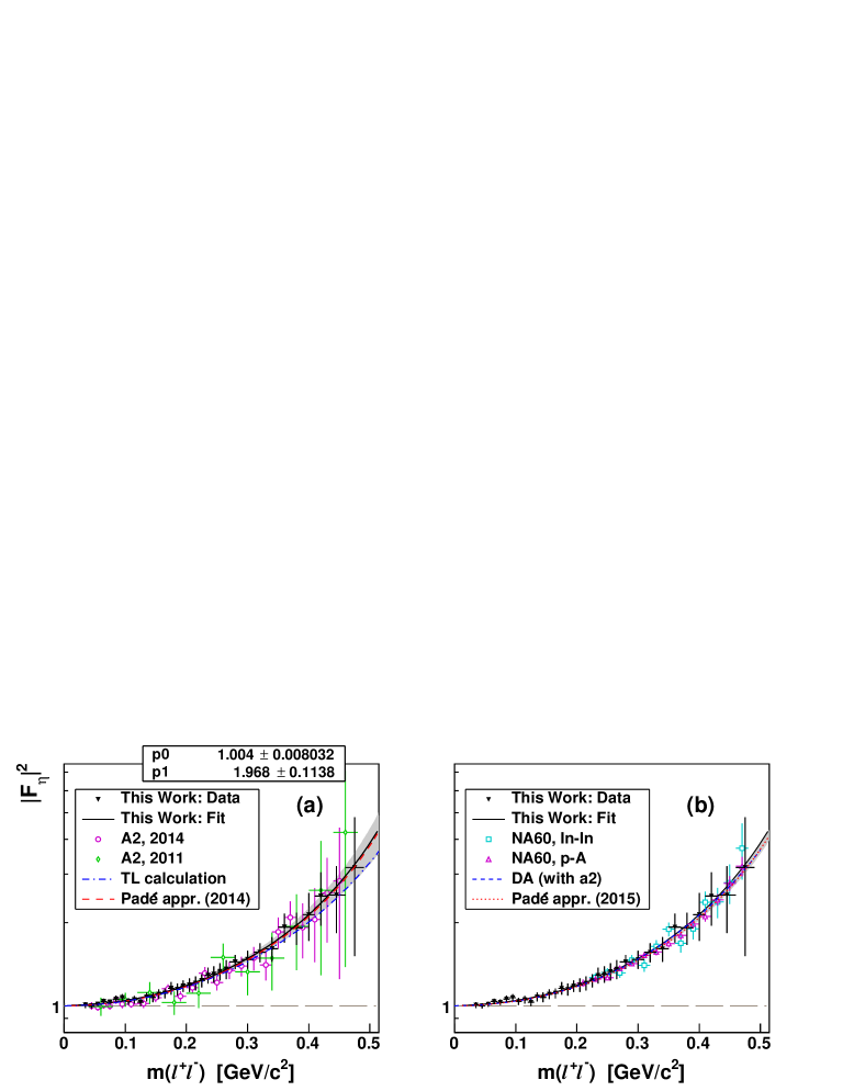
Figure 17: (Color online) $|F_{\eta}(m_{\ell^{+}\ell^{-}})|^{2}$ results (black filled triangles) combined from Run-I and Run-II and their pole-approximation fit (black solid line, with $p0$ and $p1$ being the normalization and the slope parameter $\Lambda^{-2}$, respectively) are compared to previous measurements and various theoretical calculations. The former results by the A2 Collaboration from Ref. eta_tff_a2_2014 (open magenta circles) and Ref. eta_tff_a2_2011 (open green diamonds) are shown in panel (a). The results of NA60 obtained in peripheral In–In data NA60_2009 and in p–A collisions NA60_2016 are shown in panel (b). The calculation from Ref. Ter10 is shown in (a) by a blue dash-dotted line. The most recent DA calculation by the Jülich group Xiao_2015 is shown in (b) by a blue dashed line. The calculations by the Mainz group with the Padé approximants are shown in (a) for their previous solution Esc13 (red dashed line with an error band) and in (b) for their latest solution Escribano_2015 (red dotted line with an error band).

The correlation between the two parameters results in a larger fit error for $\Lambda^{-2}$. However, this error then includes the systematic uncertainty in the general normalization of the data points. Because all $|F_{\eta}|^{2}$ results are obtained with their total uncertainties, the fit error for $\Lambda^{-2}_{\eta}$ gives its total uncertainty as well. As seen in Fig. 16, the fits to both Run-I and Run-II results give normalization parameters compatible with the expected values, indicating the good quality of the results. A value of the second parameter obtained for Run-I, $p1=(1.93\pm 0.15_{\mathrm{tot}})$ GeV^-2, is slightly smaller than the value from Ref. eta_tff_a2_2014 , $\Lambda^{-2}_{\eta}=(1.95\pm 0.15_{\mathrm{stat}}\pm 0.10_{\mathrm{syst}})=(1.95\pm 0.18_{\mathrm{tot}})$ GeV^-2, also obtained from the analysis of Run-I, but is in good agreement within the uncertainties, the magnitude of which became somewhat smaller as well. The value, $p1=(2.02\pm 0.17_{\mathrm{tot}})$ GeV^-2, obtained for Run-II is slightly larger than both the present and the previous results from Run-I, but is in good agreement within the uncertainties. The magnitude of the difference in the $\Lambda^{-2}_{\eta}$ results obtained for Run-I and Run-II is comparable to the uncertainties in the theoretical predictions for $\Lambda^{-2}_{\eta}$. As an example, the most recent calculations with the dispersive analysis (DA) by the Jülich group are shown in Fig. 16 for their new solution Xiao_2015 , obtained after including the $a_{2}$-meson contribution in the analysis, and their previous solution without it Hanhart . As seen, the fit of Run-II practically overlaps with the calculation without $a_{2}$, and the fit of Run-I is very close to the calculation involving the $a_{2}$ contribution.

The $|F_{\eta}(m_{e^{+}e^{-}})|^{2}$ results combined from Run-I and Run-II are compared to previous measurements and various theoretical calculations in Fig. 17. The numerical values for the combined $|F_{\eta}(m_{e^{+}e^{-}})|^{2}$ results are listed in Table 1. As seen in Fig. 17, the present $|F_{\eta}(m_{e^{+}e^{-}})|^{2}$ results are in good agreement, within the error bars, with all previous measurements based on $\eta\to e^{+}e^{-}\gamma$ and $\eta\to\mu^{+}\mu^{-}\gamma$ decays. The pole-approximation fit to the present $|F_{\eta}|^{2}$ data points yields

$$\Lambda^{-2}_{\eta}=(1.97\pm 0.11_{\mathrm{tot}})~{}\mathrm{GeV}^{-2},$$ (6)

which is also in very good agreement within the uncertainties with the results reported in Refs. NA60_2016 ; eta_tff_a2_2014 ; eta_tff_a2_2011 ; NA60_2009 . The uncertainty in the $\Lambda^{-2}_{\eta}$ value obtained in the present work is smaller than those of previous measurements by the A2 collaboration eta_tff_a2_2014 ; eta_tff_a2_2011 and the NA60 collaboration in peripheral In–In data NA60_2009 , but is larger than in the latest NA60 result, $\Lambda^{-2}_{\eta}=(1.934\pm 0.084_{\mathrm{tot}})$ GeV^-2, obtained from p–A collisions NA60_2016 .

Most of the theoretical calculations shown in Fig. 17 have already been discussed in Ref. eta_tff_a2_2014 . The calculation by Terschlüsen and Leupold (TL) combines the vector-meson Lagrangian proposed in Ref. Lut08 and recently extended in Ref. Ter12 , with the Wess-Zumino-Witten contact interaction Ter10 . As seen, the TL calculation lies slightly lower than the pole-approximation fit to the present data points, but is still in good agreement with the data points within their error bars. The calculations by the Jülich group, in which the radiative decay $\eta\to\pi^{+}\pi^{-}\gamma$ Stollenwerk_2012 is connected to the isovector contributions of the $\eta\to\gamma\gamma^{*}$ TFF in a model-independent way, by using dispersion theory, are shown for the latest solution Xiao_2015 , including the $a_{2}$-meson contribution in the analysis. As seen, this solution is very close to the present pole-approximation fit. The calculations by the Mainz group, which are based on a model-independent method using the Padé approximants (initially developed for the $\pi^{0}$ TFF Mas12 ), are shown for both their previous Esc13 and latest Escribano_2015 solutions. As seen, both the solutions are very close to the present pole-approximation fit. However, the latest solution, also involving the previous A2 data on the $\eta$ TFF eta_tff_a2_2014 , has a much smaller uncertainty. It is expected that adding the $|F_{\eta}(m_{e^{+}e^{-}})|^{2}$ results from this work into the corresponding calculation by the Mainz group will allow an even smaller uncertainty in the value for the slope parameter of the $\eta$ TFF to be obtained.

IV.3 comparison of $\omega$ results with other data and calculations

The individual $|F_{\omega\pi^{0}}(m_{e^{+}e^{-}})|^{2}$ results from Run-I and Run-II are compared in Fig. 18. Similarly to the comparison of the two individual sets of $|F_{\eta}(m_{\ell^{+}\ell^{-}})|^{2}$ results and their uncertainties, these experimental results are also plotted twice.

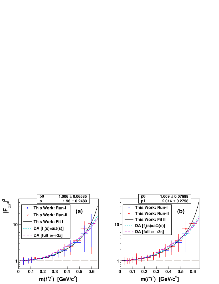
Figure 18: (Color online) Comparison of the $|F_{\omega\pi^{0}}(m_{\ell^{+}\ell^{-}})|^{2}$ results obtained individually from the analyses of Run-I (blue filled triangles) and Run-II (red open circles) with each other and with the two solutions for the DA calculations by the Bonn group Schneider_2012 shown by error-band borders. The solution using a simplified, VMD-inspired $\omega\to 3\pi$ partial wave $f_{1}(s)=\alpha\Omega(s)$ inside the dispersion integral is shown by cyan dashed lines, and the solution using the full rescattering of $3\pi$ by magenta dashed lines. The pole-approximation fits (black solid lines) to the results of Run-I and Run-II are depicted in panels (a) and (b), respectively. The fit parameter $p0$ reflects the general normalization of the data points, and $p1$ is the slope parameter $\Lambda^{-2}$. For a better comparison of the magnitudes of total uncertainties from the two data sets, the error bars of Run-I are plotted in (a) on the top of the error bars of Run-II, and the other way around in (b).

The two-parameter fits of the individual $|F_{\omega\pi^{0}}|^{2}$ results with Eq. (4) are shown in Figs. 18(a) and (b), respectively for Run-I and Run-II. As seen in Fig. 18, the experimental statistics for $\omega\to\pi^{0}e^{+}e^{-}$ decays in Run-I and Run-II and the level of background resulted in quite large total uncertainties in those $|F_{\omega\pi^{0}}|^{2}$ results, especially at large $m(e^{+}e^{-})$ masses. Within those uncertainties, the $|F_{\omega\pi^{0}}|^{2}$ results from both data sets are in good agreement with each other. The same holds for the fit results for the normalization parameter $p0$ and the parameter $p1$, corresponding to $\Lambda^{-2}_{\omega\pi^{0}}$. Despite large uncertainties in $p1=(1.96\pm 0.25_{\mathrm{tot}})$ GeV^-2 obtained for Run-I and in $p1=(2.01\pm 0.28_{\mathrm{tot}})$ GeV^-2 for Run-II, both results indicate a lower value for $\Lambda^{-2}_{\omega\pi^{0}}$ than those reported previously by Lepton-G Lepton_G_omega and NA60 NA60_2016 ; NA60_2009 . At the same time, the comparison of the individual $|F_{\omega\pi^{0}}(m_{e^{+}e^{-}})|^{2}$ results and their pole-approximation fits, for example, with the two different solutions from the dispersive analysis by the Bonn group Schneider_2012 indicates no contradiction with these calculations.

The $|F_{\omega\pi^{0}}(m_{e^{+}e^{-}})|^{2}$ results combined from Run-I and Run-II are compared to previous measurements and various theoretical calculations in Fig. 19. The numerical values for the combined $|F_{\omega\pi^{0}}(m_{e^{+}e^{-}})|^{2}$ results are listed in Table 2.

Table 2: Results of this work for the $\omega\pi^{0}$ TFF, $|F_{\omega\pi^{0}}|^{2}$, as a function of the invariant mass $m(e^{+}e^{-})$.

$m(e^{+}e^{-})$ [MeV/$c^{2}$]	$40\pm 10$	$60\pm 10$	$80\pm 10$	$105\pm 15$	$135\pm 15$	$175\pm 25$	$225\pm 25$
$|F_{\omega\pi^{0}}|^{2}$	$1.002\pm 0.162$	$1.011\pm 0.120$	$1.027\pm 0.121$	$1.058\pm 0.140$	$1.126\pm 0.239$	$1.146\pm 0.128$	$1.227\pm 0.161$
$m(e^{+}e^{-})$ [MeV/$c^{2}$]	$275\pm 25$	$325\pm 25$	$375\pm 25$	$425\pm 25$	$480\pm 30$	$540\pm 30$	$600\pm 30$
$|F_{\omega\pi^{0}}|^{2}$	$1.390\pm 0.215$	$1.648\pm 0.279$	$1.946\pm 0.431$	$2.553\pm 0.692$	$3.32\pm 1.08$	$6.32\pm 2.90$	$10.63\pm 6.14$

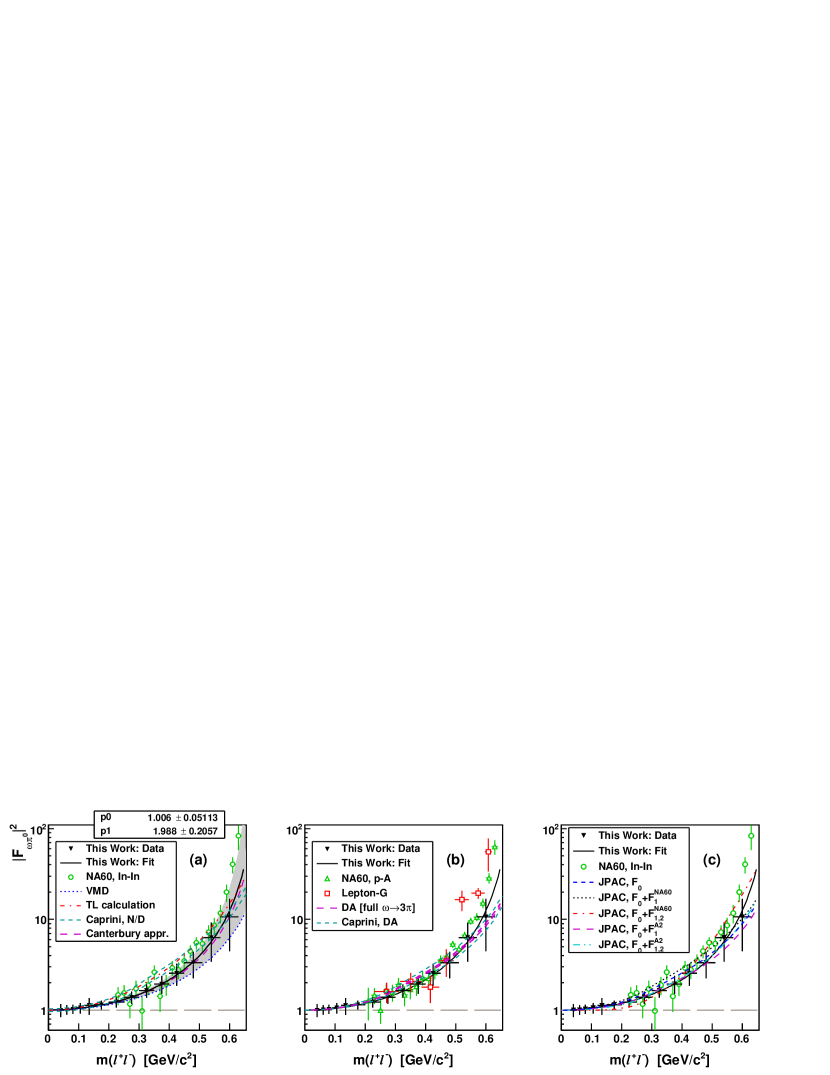
Figure 19: (Color online) $|F_{\omega\pi^{0}}(m_{\ell^{+}\ell^{-}})|^{2}$ results (black filled triangles) combined from Run-I and Run-II and their pole-approximation fit (black solid line, with $p0$ and $p1$ being the normalization and the slope parameter $\Lambda^{-2}$, respectively) are compared to previous measurements and various theoretical calculations. The results by Lepton-G Lepton_G_omega are shown by open red squares in panel (b). The results of NA60 obtained in peripheral In–In data NA60_2009 are shown by open green circles in (a) and (c), and from p–A collisions NA60_2016 by open green triangles in (b). The VMD prediction is shown by a blue dashed line in (a). The calculation from Refs. TL10 ; Ter12 is shown by a red dash-dotted line in (a). The DA calculation by the Bonn group Schneider_2012 for the full $3\pi$ rescattering is shown by error-band borders (magenta dashed lines) in (b). Upper and lower bounds by Caprini Caprini_2015 are shown by cyan dashed lines for two cases of the discontinuity calculated with the partial-wave amplitude $f_{1}(t)$ based on the improved N/D model Koepp_1974 (a), and taken from Ref. Schneider_2012 (b). The calculation based on a model-independent method using Canterbury approximants Pere_2016 is shown by a magenta long-dashed line with a gray error band. The basic calculation (blue dashed line) from JPAC Danilkin_2015 and the effect from including higher order terms of the inelastic contributions in the $\omega\pi^{0}$ TFF by fitting them to the NA60 In–In data is shown in (c) for the solutions with adding one (black dotted line) and two (red dash-dotted line) terms. A similar effect from including higher order terms by fitting them to the present $|F_{\omega\pi^{0}}(m_{\ell^{+}\ell^{-}})|^{2}$ results is shown in (c) for the solutions with one (magenta long-dashed line) and with two (cyan dash-double-dotted line) terms.

As seen in Fig. 19, the present $|F_{\omega\pi^{0}}(m_{e^{+}e^{-}})|^{2}$ results are in general agreement, within the error bars, with the previous measurements based on $\omega\to\pi^{0}\mu^{+}\mu^{-}$ decays. The only deviation observed is for the data points at the largest $m(e^{+}e^{-})$ masses. The pole-approximation fit to the present $|F_{\omega\pi^{0}}|^{2}$ data points gives

$$\Lambda^{-2}_{\omega\pi^{0}}=(1.99\pm 0.21_{\mathrm{tot}})~{}\mathrm{GeV}^{-2},$$ (7)

which is somewhat lower than the corresponding value obtained from the Lepton-G and NA60 data Lepton_G_omega ; NA60_2016 ; NA60_2009 , but does not contradict them within the uncertainties. The uncertainty in the $\Lambda^{-2}_{\omega\pi^{0}}$ value obtained in the present work is similar to that of Lepton-G, but is significantly larger than the accuracy achieved by NA60. Meanwhile, the advantage in measuring the $\omega\to\pi^{0}e^{+}e^{-}$ decay is that the control of the overall normalization of the $|F_{\omega\pi^{0}}|^{2}$ results is much more stringent than in the case of the $\omega\to\pi^{0}\mu^{+}\mu^{-}$ decay, which does not enable measurement at low $m(\ell^{+}\ell^{-})$. The magnitude of the parameter $p0$, obtained from the fit to the present $|F_{\omega\pi^{0}}|^{2}$ results, indicates small values of systematic uncertainties due to the normalization, which depends on the correctness in the reconstruction of both the $\omega\to\pi^{0}e^{+}e^{-}$ and $\omega\to\pi^{0}\gamma$ decays as well as on radiative corrections for the QED differential decay rate at low $q$. As noted previously, the magnitude of those corrections is expected to be $\sim$1%.

The basic ideas of the theoretical calculations shown in Fig. 19 have already been discussed in the Introduction. The calculation from Refs. TL10 ; Ter12 is shown by a red dash-dotted line in Fig. 19(a). The DA calculation by the Bonn group Schneider_2012 is shown in Fig. 19(b) by error-band borders (magenta dashed lines) for the solution with the full $3\pi$ rescattering. The calculations by Caprini Caprini_2015 are shown for two cases. Upper and lower bounds calculated with the discontinuity using the partial-wave amplitude $f_{1}(t)$ from Ref. Schneider_2012 are shown in Fig. 19(b). And bounds obtained with the improved N/D model Koepp_1974 for $f_{1}(t)$ are shown in Fig. 19(a).

There is another $\omega\pi^{0}$-TFF prediction translated to a simple monopole form of Eq. (4) with the parameter $\Lambda=(0.72\pm 0.05)$ GeV, or $\Lambda^{-2}=(1.93\pm 0.26)$ GeV^-2 Pere_2016 , which is depicted by a magenta long-dashed line with a gray error band in Fig. 19(a). This calculation is based on a model-independent method using Canterbury approximants, which are an extension of the Padé theory for bivariate functions Pere_2015 . The parameter $\Lambda$ is obtained by requiring that the slope of the $\omega\pi^{0}$ TFF in the variable $q^{2}$ should be the same as for the $\pi^{0}$ TFF, taking into account isospin breaking. In the approach used, the $\omega\pi^{0}$ TFF is considered as the $\pi^{0}$ TFF of double virtuality, with the virtuality of one of the photons fixed to the $\omega$-meson mass, and the other photon to the invariant mass of the lepton pair. The relatively large uncertainty in this prediction at higher $m(\ell^{+}\ell^{-})$ is determined by the uncertainty in the $\pi^{0}$ TFF extrapolated in the region of larger $q^{2}$.

Among the calculations depicted in Figs. 19(a) and (b), those by the Bonn group and by Caprini with the $f_{1}(t)$ amplitude from the same work Schneider_2012 seem to be in reasonable agreement with the present data points. The prediction based on the method using Canterbury approximants is fairly close to the curve showing the data fit, but the uncertainty in this prediction at higher $m(\ell^{+}\ell^{-})$ is larger, compared to the other calculations. Although the magnitude of the uncertainties in the present $|F_{\omega\pi^{0}}|^{2}$ results does not allow ruling out any of the calculations shown, it does challenge the understanding of the energy dependence of the $\omega\pi^{0}$ TFF at intermediate and high $q^{2}$.

The calculations made for $|F_{\omega\pi^{0}}|^{2}$ by the Joint Physics Analysis Center (JPAC) Danilkin_2015 and also the two new solutions, involving a fit to the present results, are shown in Fig. 19(c). The basic calculation (shown by a blue dashed line) was obtained by using only the first term in the expansion of the inelastic contribution in terms of conformal variables $\omega^{i}(s)$, with its weight parameter determined from the experimental value for $\Gamma(\omega\to\pi^{0}\gamma)$. Other solutions were obtained by including higher-order inelastic-contribution terms (the next one or two orders) in the $\omega\pi^{0}$ TFF by fitting their parameters to the experimental $|F_{\omega\pi^{0}}|^{2}$ data. The solutions with fits to the NA60 In–In data are shown by a black dotted line for one additional term, and by a red dash-dotted line for two. The solutions with fits to the present data are shown by a magenta long-dashed line for one additional term, and by a cyan dash-double-dotted line for two. As seen in Fig. 19(c), the basic calculation from Ref. Danilkin_2015 lies below the NA60 In–In data points at large $m(\ell^{+}\ell^{-})$ masses, but comes very close to the data points of the present measurement. Including one more $\omega^{i}(s)$ term, with fitting its weight to the data, does not change much for either the NA60 In–In or the present results. Including two additional $\omega^{i}(s)$ terms in the fitting to the NA60 In–In data results in a better agreement with their results, but it is difficult to justify such a strong rise of the inelastic form factor Caprini_2014 . For the present data, the solution with two additional $\omega^{i}(s)$ terms is very close to the basic calculation, which agrees with the small magnitude expected for higher-order terms of the inelastic contributions.

Thus, the results of the present work for $|F_{\omega\pi^{0}}|^{2}$ indicate a better agreement with existing theoretical calculations than observed for previous measurements. Although the statistical accuracy of the present data points at large $m(\ell^{+}\ell^{-})$ masses does not allow a final conclusion to be drawn regarding the energy dependence of the $\omega\pi^{0}$ TFF in this region, the present $|F_{\omega\pi^{0}}|^{2}$ results for intermediate $m(\ell^{+}\ell^{-})$ masses obviously do not favor some of the calculations. More measurements of the $\omega\to\pi^{0}e^{+}e^{-}$ decay, with much better statistical accuracy, especially at large $m(\ell^{+}\ell^{-})$ masses, are needed to solve the problem of the inconsistency remaining between the calculations and the experimental data. Once the agreement between the theory and the experiment is established for the $\omega\to\pi^{0}\gamma^{*}$ TFF, or the origin of the potential disagreement is understood, then such data could make an improvement in the theoretical uncertainties, in particular the dispersive model-independent calculations and the Padé-approximants method, which could then result in a better determination of the corresponding HLbL contribution to $(g-2)_{\mu}$.

A better knowledge of radiative corrections for QED differential decay rates of Dalitz decays will be important for more reliable TFF measurements. It was checked in the present analysis that the correction for the QED energy dependence makes this dependence lower by $\sim$10% at the largest $q$ measured. However, because the radiative corrections suppress the decay amplitude at extreme $\cos\theta^{*}$, taken together with the lower acceptance for those angles, the detection efficiency improves at large $q$. This partially compensates the impact from using lower QED values for measuring TFFs at large $q$.

V Summary and conclusions

The Dalitz decays $\eta\to e^{+}e^{-}\gamma$ and $\omega\to\pi^{0}e^{+}e^{-}$ have been measured in the $\gamma p\to\eta p$ and $\gamma p\to\omega p$ reactions, respectively, with the A2 tagged-photon facility at the Mainz Microtron, MAMI. The value obtained for the slope parameter of the $\eta$ e/m TFF, $\Lambda^{-2}_{\eta}=(1.97\pm 0.11_{\mathrm{tot}})$ GeV^-2, is in good agreement with previous measurements of the $\eta\to e^{+}e^{-}\gamma$ and $\eta\to\mu^{+}\mu^{-}\gamma$ decays, and the $|F_{\eta}|^{2}$ results are in good agreement with recent theoretical calculations. The uncertainty obtained in the value of $\Lambda^{-2}_{\eta}$ is lower than in previous results based on the $\eta\to e^{+}e^{-}\gamma$ decay and the NA60 result based on $\eta\to\mu^{+}\mu^{-}\gamma$ decays from peripheral In–In collisions. The value obtained for $\omega$, $\Lambda^{-2}_{\omega\pi^{0}}=(1.99\pm 0.21_{\mathrm{tot}})$ GeV^-2, is somewhat lower than previous measurements based on the $\omega\to\pi^{0}\mu^{+}\mu^{-}$ decay. The results of this work for $|F_{\omega\pi^{0}}|^{2}$ are in better agreement with theoretical calculations than the data from earlier experiments. However, the statistical accuracy of the present data points at large $m(e^{+}e^{-})$ masses does not allow a final conclusion to be drawn about the energy dependence in this region. More measurements of the $\omega\to\pi^{0}e^{+}e^{-}$ decay, with much better statistical accuracy, especially at large $m(e^{+}e^{-})$ masses, are needed to solve the problem in the inconsistency remaining between the calculations and the experimental data. Compared to the $\eta\to\mu^{+}\mu^{-}\gamma$ and $\omega\to\pi^{0}\mu^{+}\mu^{-}$ decays, measuring $\eta\to e^{+}e^{-}\gamma$ and $\omega\to\pi^{0}e^{+}e^{-}$ decays gives access to the TFF energy dependence at low momentum transfer, which is important for data-driven approaches calculating the corresponding rare decays and the HLbL contribution to $(g-2)_{\mu}$.

References

- (1) Proceedings of the First MesonNet Workshop on Meson Transition Form Factors, 2012, Cracow, Poland, edited by E. Czerwinski, S. Eidelman, C. Hanhart, B. Kubis, A. Kupść, S. Leupold, P. Moskal, and S. Schadmand, arXiv:1207.6556 [hep-ph].
- (2) G. Colangelo, M. Hoferichter, B. Kubis, M. Procura, and P. Stoffer, Phys. Lett. B 738, 6 (2014).
- (3) G. Colangelo, M. Hoferichter, M. Procura, and P. Stoffer, J. High Energy Phys. 09 (2015) 074.
- (4) F. Jegerlehner and A. Nyffeler, Phys. Rep. 477, 1 (2009).
- (5) A. Nyffeler, Phys. Rev. D 94, 053006 (2016).
- (6) V. Pauk and M. Vanderhaeghen, Phys. Rev. D 90, 113012 (2014).
- (7) T. Husek and S. Leupold, Eur. Phys. J. C 75, 586 (2015).
- (8) P. Masjuan and P. Sanchez-Puertas, J. High Energy Phys. 08 (2016) 108.
- (9) N. M. Kroll and W. Wada, Phys. Rev. 98, 1355 (1955).
- (10) L. G. Landsberg, Phys. Rep. 128, 301 (1985).
- (11) J. J. Sakurai, Currents and mesons, University of Chicago Press, Chicago, USA, 1969.
- (12) R. Arnaldi et al., Phys. Lett. B 757, 47 (2016).
- (13) T. Husek, K. Kampf, and J. Novotný, Phys. Rev. D 92, 054027 (2015).
- (14) R. I. Dzhelyadin et al., Phys. Lett. B 94, 548 (1980).
- (15) R. Arnaldi et al., Phys. Lett. B 677, 260 (2009).
- (16) H. Berghäuser et al., Phys. Lett. B 701, 562 (2011).
- (17) P. Aguar-Bartolome et al. Phys. Rev. C 89, 044608 (2014).
- (18) R. Escribano, P. Masjuan, and P. Sanchez-Puertas, Eur. Phys. J. C 75, 414 (2015).
- (19) P. Sanchez-Puertas and P. Masjuan, arXiv:1510.05607 [hep-ph].
- (20) C. W. Xiao, T. Dato, C. Hanhart, B. Kubis, U.-G. Meißner, and A. Wirzba, arXiv:1509.02194 [hep-ph].
- (21) C. Hanhart, A. Kupść, U.-G. Meißner, F. Stollenwerk, and A. Wirzba, Eur. Phys. J. C 73, 2668 (2013); ibid. 75, 242 (2015).
- (22) B. Kubis and J. Plenter, Eur. Phys. J. C 75, 283 (2015).
- (23) R. I. Dzhelyadin et al., Phys. Lett. B 102, 296 (1981).
- (24) C. Terschlüsen and S. Leupold, Phys. Lett. B 691, 191 (2010).
- (25) C. Terschlüsen, S. Leupold, and M. F. M. Lutz, Eur. Phys. J. A 48, 190 (2012).
- (26) S. P. Schneider, B. Kubis, and F. Niecknig, Phys. Rev. D 86, 054013 (2012).
- (27) I. V. Danilkin, C. Fernández-Ramírez, P. Guo, V. Mathieu, D. Schott, M. Shi, and A. P. Szczepaniak, Phys. Rev. D 91, 094029 (2015).
- (28) F. Niecknig, B. Kubis, and S. P. Schneider, Eur. Phys. J. C 72, 2014 (2012)
- (29) B. Ananthanarayan, I. Caprini, and B. Kubis, Eur. Phys. J. C 74, 3209 (2014).
- (30) I. Caprini, Phys. Rev. D 92, 014014 (2015).
- (31) B. M. K. Nefkens et al., Phys. Rev. C 90, 025206 (2014).
- (32) A. Starostin et al., Phys. Rev. C 64, 055205 (2001).
- (33) R. Novotny, IEEE Trans. Nucl. Sci. 38, 379 (1991).
- (34) A. R. Gabler et al., Nucl. Instrum. Methods Phys. Res. A 346, 168 (1994).
- (35) H. Herminghaus et al., IEEE Trans. Nucl. Sci. 30, 3274 (1983).
- (36) K.-H. Kaiser et al., Nucl. Instrum. Methods Phys. Res. A 593, 159 (2008).
- (37) I. Anthony et al., Nucl. Instrum. Methods Phys. Res. A 301, 230 (1991).
- (38) S. J. Hall et al., Nucl. Instrum. Methods Phys. Res. A 368, 698 (1996).
- (39) J. C. McGeorge et al., Eur. Phys. J. A 37, 129 (2008).
- (40) S. Prakhov et al., Phys. Rev. C 79, 035204 (2009).
- (41) E. F. McNicoll et al., Phys. Rev. C 82, 035208 (2010).
- (42) A. Nikolaev et al., Eur. Phys. J. A 50, 58 (2014).
- (43) D. Watts, Proceedings of the 11th International Conference on Calorimetry in Particle Physics, Perugia, Italy, 2004 (World Scientific, Singapore, 2005), p. 560.
- (44) I. I. Strakovsky et al., Phys. Rev. C 91, 045207 (2015).
- (45) K. A. Olive et al., (Particle Data Group), Chin. Phys. C 38, 090001 (2014).
- (46) V. L. Kashevarov et al., Phys. Rev. C 85, 064610 (2012).
- (47) M. F. M. Lutz and S. Leupold, Nucl. Phys. A 813, 96 (2008).
- (48) C. Terschlüsen, Diploma Thesis, University of Gießen, 2010.
- (49) F. Stollenwerk, C. Hanhart, A. Kupść, U.-G. Meißner, and A. Wirzba, Phys. Lett. B 707, 184 (2012).
- (50) P. Masjuan, Phys. Rev. D 86, 094021 (2012).
- (51) R. Escribano, P. Masjuan, and P. Sanchez-Puertas, Phys. Rev. D 89, 034014 (2014).
- (52) G. Köpp, Phys. Rev. D 10, 932 (1974).
- (53) P. Masjuan, private communication.
- (54) P. Masjuan and P. Sanchez-Puertas, arXiv:1504.07001 [hep-ph].