53 Avenue des Martyrs, 38026 Grenoble, France 55institutetext: Theoretische Natuurkunde and IIHE/ELEM, Vrije Universiteit Brussel, and International Solvay Institutes,
Pleinlaan 2, 1050 Brussels, Belgium 66institutetext: Department of Physics and Astronomy, University of Sussex, Brighton BN1 9QH, UK 77institutetext: Centre for Cosmology, Particle Physics and Phenomenology (CP3), Université catholique de Louvain,
Chemin du Cyclotron, 1348 Louvain-la-Neuve, Belgium
Electroweak Higgs boson production in the standard model effective field theory beyond leading order in QCD
Abstract
We study the impact of dimension-six operators of the standard model effective field theory relevant for vector-boson fusion and associated Higgs boson production at the LHC. We present predictions at the next-to-leading order accuracy in QCD that include matching to parton showers and that rely on fully automated simulations. We show the importance of the subsequent reduction of the theoretical uncertainties in improving the possible discrimination between effective field theory and standard model results, and we demonstrate that the range of the Wilson coefficient values allowed by a global fit to LEP and LHC Run I data can be further constrained by LHC Run II future results.
IPPP/16/80, LPSC16198
1 Introduction
The LHC Run I and early Run II data have not yet put forward any strong evidence of physics beyond the standard model (SM) and limits on new states have instead been pushed to higher and higher energies. As a consequence, the effective field theory (EFT) extension of the SM (SMEFT) has become increasingly relevant. The SMEFT is built from the SM symmetries and degrees of freedom (including the Higgs sector) by adding new operators of dimension higher than four to the SM Lagrangian. Being a tool to parameterise the search for new anomalous interactions, it is fully complementary to direct searches for new particles. Interpreting data in the context of the SMEFT hence allows us to be sensitive to new physics beyond the current energy reach of the LHC in a model-independent way.
The formulation of the effective Lagrangian restricted to operators of dimension of at most six relies on the definition of a complete and non-redundant operator basis Grzadkowski:2010es ; Contino:2013kra ; Gupta:2014rxa and should additionally include the translations among the possible choices Falkowski:2015wza . This has been intensively discussed and will be soon reported by the Higgs cross section working group YR4 . Moreover, since we try to observe small deviations from the SM, precise theoretical predictions are required both in the SM and in the SMEFT framework. The accumulation of LHC data and the subsequent precision obtained indeed call for a similar accuracy on the theoretical side, which demands the inclusion of higher-order corrections.
What we present in this paper is a part of the current theoretical activities aiming for precision predictions for electroweak Higgs-boson production at the LHC, i.e. Higgs boson production in association with a weak boson (VH) and via vector-boson fusion (VBF). In this context, NLO+PS (next-to-leading order plus parton-shower) matched predictions for VH and VBF production in the SM have been released both in the MC@NLO Frixione:2002ik ; LatundeDada:2009rr ; Frixione:2013mta and Powheg Nason:2004rx ; Hamilton:2009za ; Nason:2009ai frameworks, and merged NLO samples describing VH production including up to one additional jet have been generated in both the Powheg Luisoni:2013kna and Sherpa Goncalves:2015mfa platforms. NLO QCD corrections along with the inclusion of anomalous interactions have been further investigated for VH Campanario:2014lza and VBF Hankele:2006ma Higgs boson production, and matched to parton showers in the Higgs characterisation framework Artoisenet:2013puc ; Maltoni:2013sma . Finally, electroweak corrections as well as anomalous coupling effects for VH production have been included in the Hawk program Denner:2011id that also contains NLO QCD contributions. In contrast, fixed-order predictions are known to a higher accuracy for both VH and VBF SM Higgs production processes Kumar:2014uwa ; Campbell:2016jau ; Dreyer:2016oyx ; Cacciari:2015jma .
In the SMEFT framework (in contrast to the anomalous coupling approach), the VH process has been studied at the NLO+PS accuracy within the Powheg-Box framework Mimasu:2015nqa , where a subset of the 59 independent dimension-six operators was taken into account. In this paper, similarly, we consider five operators which are relevant for VH production. Firstly, we independently provide NLO+PS predictions for the VH process by using a different framework via a joint use of FeynRules Alloul:2013bka , NloCT Degrande:2014vpa and MadGraph5_aMC@NLO (MG5_aMC) Alwall:2014hca programs. This approach provides a fully automatic procedure linking the model Lagrangian to event generation matched to parton showers at NLO. Our work hence not only independently validates the previous results obtained with Powheg-Box but also includes the additional benefits stemming from the flexibility of the FeynRules program. As a result, one can exploit generators like MG5_aMC for simulating any desired process at the NLO+PS accuracy (i.e. the VBF process in our case) for which the same operators play a role. This is the second part of our paper, which presents the first SMEFT results for this process. Although we only present results for a couple of benchmark scenarios motivated by global fit results, our predictions can be straightforwardly generalised to any scenario by using our public Universal FeynRules Output (UFO) model FR-HEL:Online within MG5_aMC Christensen:2009jx ; Degrande:2011ua ; deAquino:2011ub .
We emphasise that, following some recent results in the channel Maltoni:2016yxb , this work represents a step towards a complete SMEFT operator basis implementation for Higgs physics at the NLO QCD accuracy, which will be beneficial to both the theoretical and experimental communities.
In Sect. 2 we provide the necessary theoretical ingredients to calculate NLO-QCD corrections for VH and VBF Higgs production in the SMEFT. We also discuss current constraints on the Wilson coefficients originating from a LEP and LHC Run I global fit analysis with which we inform our benchmark point selection. In Sect. 3 we describe our setup for NLO computations matched to parton showers. We present our numerical results in Sects. 4 and 5, and also assess the validity of the EFT given the current constraints on the Wilson coefficients. We asses the reach of the future LHC reach in Sect. 6, before concluding in Sect. 7. Practical information for event simulation and model validations are provided in the appendix.
2 Theoretical framework
2.1 Model description
In the SM of particle physics, the elementary particles and their interactions are described by a quantum field theory based on the gauge symmetry. The vector fields mediating the gauge interactions lie in the adjoint representation of the relevant gauge group,
| (1) |
where the notations for the representation refer to the full SM symmetry group. The chiral content of the theory is defined by three generations of left-handed and right-handed quark (, and ) and lepton ( and ) fields whose representation under the SM gauge group is given by
| (2) |
The Higgs sector contains a single doublet of fields that is responsible for the breaking of electroweak symmetry,
| (3) |
where the components of the doublet are given in terms of the physical Higgs field shifted by its vacuum expectation value and the Goldstone bosons and that are eaten by the weak bosons to give them their longitudinal degree of freedom.
In the EFT framework, new physics is expected to appear at a scale large enough so that the new degrees of freedom can be integrated out. As a result, the SM Lagrangian is supplemented by higher-dimensional operators parameterising all effects beyond the SM,
| (4) |
Restricting ourselves to operators of dimension six, the most general gauge-invariant Lagrangian has been known for a long time Burges:1983zg ; Leung:1984ni ; Buchmuller:1985jz and can be expressed in a suitable form by choosing a convenient basis of independent operators Grzadkowski:2010es ; Contino:2013kra ; Gupta:2014rxa . In this work, we focus on five specific, bosonic operators,111The relevant fermionic operators are also considered in, e.g., Ge:2016zro . which are relevant to the VH and VBF processes, taken from the strongly interacting light Higgs (SILH) basis Giudice:2007fh ; Contino:2013kra ; Alloul:2013naa ,222Although the -boson mass and are usually used as expansion parameters in this basis, our model explicitly uses a cutoff scale . For all our numerical results, we set . We also point out a relative factor 2 difference in our definition of and with respect to Refs. Giudice:2007fh ; Contino:2013kra ; Alloul:2013naa .
| (5) |
The Wilson coefficients are free parameters, are the generators of (with ) in the fundamental representation and the Hermitian derivative operators are defined by
| (6) |
In our conventions, the gauge-covariant derivatives and the gauge field strength tensors read
| (7) |
where are the structure constants of . In addition, and denote the coupling constants of and respectively.
After the breaking of the electroweak symmetry down to electromagnetism, the weak and hypercharge gauge eigenstates mix to the physical -boson, -boson and the photon ,
| (8) |
We have introduced in this expression the sine and cosine of the weak mixing angle and which diagonalise the neutral electroweak gauge boson mass matrix. The higher-dimensional operators of Eq. (5) induce a modification of the gauge boson kinetic terms that become, in the mass basis and after integration by parts,
| (9) |
where , and denote the -boson, -boson and photon field strength tensors, respectively. Consequently, canonical normalisation has to be restored by redefining the electroweak boson fields,
| (10) |
We have made use here of the freedom related to the removal of the photon and -boson mixing terms induced by the higher-order operators. This mixing can indeed be absorbed either in a photon field redefinition, or in a -boson field redefinition, or in both (as in Eq. (10)). In order to minimise the modification of the weak interactions with respect to the SM, we additionally redefine the weak and hypercharge coupling constants
| (11) |
As a result of this choice, the relations between the measured values for the electroweak inputs and all internal electroweak parameters are simplified. The -boson mass is now given by
| (12) |
while the photon stays massless and the expression of the -boson mass is unchanged respect to the SM one.
We define the electroweak sector of the theory in terms of the Fermi coupling constant as extracted from the muon decay data, the measured -boson mass and the electromagnetic coupling constant in the low-energy limit of the Compton scattering. The vacuum expectation value of the Higgs field can therefore be derived from the Fermi constant as in the SM, . After the field redefinitions of Eq. (10), the electromagnetic interactions of the fermions to the photon field turn out to be solely modified by the operator, so that the electromagnetic coupling constant is related to the input parameter as
| (13) |
Furthermore, the shift in the cosine of the Weinberg mixing angle can be derived, at first order in , from the -boson mass relation of Eq. (12) along with Eq. (13),
| (14) |
with , and
| (15) |
As a consequence, the and parameters are constrained by the measurement of the -boson mass and by the -boson decay data. Those constraints can nonetheless be modified if other dimension-six operators are added to the Lagrangian of Eq. (5).
| Eq. (16) | Our conventions | Ref. Alloul:2013naa (HEL) | Ref. Artoisenet:2013puc (HC) |
|---|---|---|---|
| + | |||
In unitary gauge and rotating all field to the mass basis, all three-point interactions involving a single (physical) Higgs boson and a pair of electroweak gauge bosons are given by
| (16) |
where integration by parts has been used to reduce the number of independent Lorentz structures. Table 1 shows the relation between the couplings in Eq. (16) and the Wilson coefficients in Eq. (5). As a reference, we also compare our conventions to those of the previous SILH Lagrangian implementation of Ref. Alloul:2013naa and of the Higgs characterisation Lagrangian of Ref. Artoisenet:2013puc .
2.2 Constraints from global fits of LEP and LHC Run I data
In this section we summarise the current bounds on the Wilson coefficients associated with the effective operators under consideration.
We start from the results of previous works Ellis:2014jta ; Ellis:2014dva , where a global fit to LEP and LHC Run I data has been performed. The results imply constraints on several linear combinations of the coefficients appearing in Eq. (5) that we present in Table 2, each limit having been obtained by marginalising over all other coefficients. Leading-order (LO) theoretical predictions have been used and in addition, the modifications of the electroweak parameters computed in Eq. (13) and Eq. (14) have not been considered for LHC predictions. We have nevertheless checked that the corresponding effects are small compared with the LHC Run I sensitivity, as also noted by the ATLAS collaboration Aad:2015tna .
| Coefficients | Bounds |
|---|---|
In many classes of SM extensions (featuring in particular an extended Higgs sector), certain relations among the coefficients appear. For instance, it is common that matching conditions such that appear Gorbahn:2015gxa . In this case, the global fit generates the more stringent constraint when one sets the effective scale to Ellis:2014jta .
2.3 Benchmark points
For both production processes of interest, we consider two benchmark scenarios in the Wilson coefficient parameter space. These two points are selected to be compatible with the global fit results discussed in Sect. 2.2.
We first make use of the fact that, as seen in Table 2, electroweak precision observables strongly constrain a particular linear combination of the and Wilson coefficients beyond a precision than can be hoped for at the LHC. We therefore impose , which in turn leads to an allowed range (setting ) for of , as obtained from the second constraint on these two parameters. In order to highlight the impact of the two new Lorentz structures appearing in the interaction vertices of the Lagrangian of Eq. (16), we allow for non-zero values for both the and coefficients.
Our benchmark scenarios are defined in Table 3. In the first setup, we only switch on the operator (which induces new physics contributions to both the and structures). With the second point, we additionally fix to an equal and opposite value relying on the constraint relation brought up in Sect. 2.2. This allows for turning on solely the coupling (see Table 1).
| Benchmarks | |||
|---|---|---|---|
| A: | 0.03 | 0 | 0 |
| B: | 0.03 | 0.015 |
3 Setup for NLO+PS simulations
Our numerical results are derived at the NLO accuracy in QCD thanks to a joint use of the FeynRules/NloCT and MG5_aMC packages. The EFT Lagrangian of Eq. (5) has been implemented in FeynRules Alloul:2013bka , while the computation of the ultraviolet counterterms and the rational terms necessary for numerical loop-integral evaluation has been done by NloCT Degrande:2014vpa that relies on FeynArts Hahn:2000kx . The model information is then provided to MG5_aMC Alwall:2014hca in the UFO format Degrande:2011ua . Within MG5_aMC, loop-diagram contributions are numerically evaluated Hirschi:2011pa and combined with the real emission pieces within the FKS subtraction scheme Frixione:1995ms ; Frederix:2009yq . Short-distance events are finally matched to parton showers according to the MC@NLO prescription Frixione:2002ik .
We generate events for 13 TeV LHC collisions using the LO and NLO NNPDF2.3 set of parton densities Ball:2013hta for LO and NLO simulations, respectively. Events are then showered and hadronised within the Pythia8 infrastructure Sjostrand:2007gs , which is also used for handling Higgs-boson decays. This latter step relies on eHdecay Contino:2014aaa that computes all branching fractions of the Higgs boson into the relevant final states to the first order in the Wilson coefficients. This procedure has the advantage of providing a correct normalisation for the production rates that includes all effects originating from the EFT operators. For the two adopted benchmark points, the deviations from the SM branching ratios are found to be very small.
Event reconstruction and analysis are performed using the MadAnalysis5 Conte:2012fm framework, which makes use of all jet algorithms implemented in the FastJet program Cacciari:2011ma . Jets are defined using the anti- algorithm Cacciari:2008gp with a radius parameter of 0.4.
Theoretical uncertainties due to renormalisation () and factorisation () scale variations are accounted for thanks to the reweighting features of MG5_aMC Frederix:2011ss . At the event generation stage, nine alternative weights are stored for each event, corresponding to the independent variation of the two scales by a factor of two up and down with respect to a central scale . Since the parton shower is unitary, these could be used to reweight the events after showering and reconstruction, saving a great deal of computational time and storage. The scale variation uncertainty is taken to be the largest difference between the central scale and the alternative scale choice predictions. We use as a central scale and for VH and VBF processes, respectively, where is defined at the parton-level as the scalar sum of the transverse momentum of all visible final-state particles and the missing transverse energy. We refer the reader to the appendix for further technical details on event generation.
4 Higgs production in association with a vector boson
Higgs-boson production in association with a vector boson is an excellent probe for new physics, as the momentum transfer in the process is directly sensitive to the Lorentz structure appearing in the interaction vertices Ellis:2012xd . The use of differential information at the LHC Run I has therefore enhanced the sensitivity of Higgs data to possible new physics effects Ellis:2014dva . Those Run I studies have, however, relied on predictions evaluated at the LO accuracy in QCD. With the improved capabilities of the LHC Run II, NLO QCD effects become more relevant and more precise predictions are in order.
To showcase our NLO simulation setup for associated VH production, we study various differential distributions in the
| (17) |
channel, where stands for the final-state missing energy. We impose the requirement that both -jets and leptons have a pseudorapidity, , and a transverse momentum, , satisfying and GeV, respectively, while non--tagged jets are instead allowed to be more forward, with , for the same requirement. We select events by demanding the presence of one lepton and two -jets based on truth-level hadronic information, a -tagged jet being defined by the presence of a -hadron within a cone of radius centred on the jet direction.
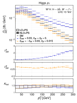
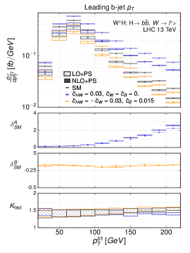
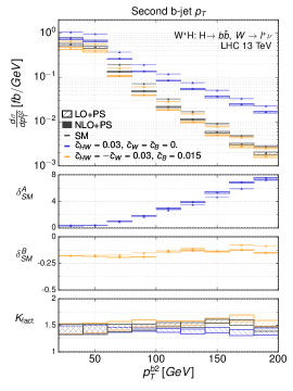
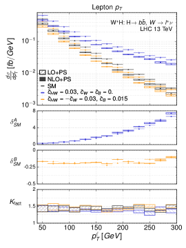
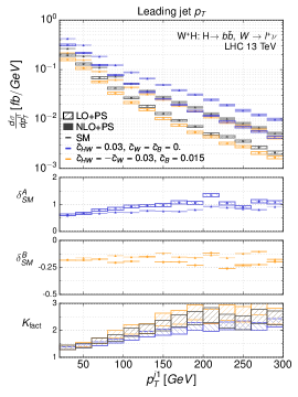
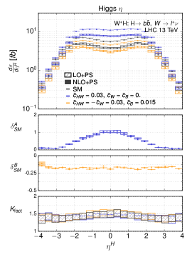
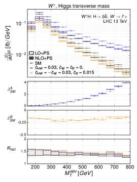
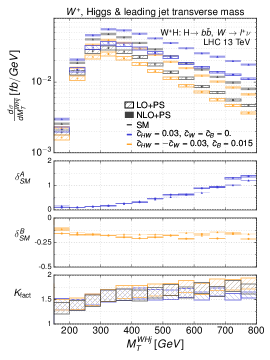
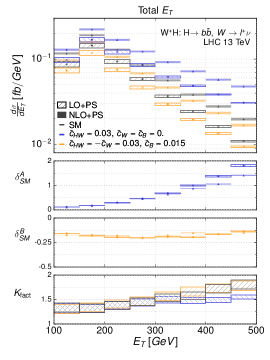
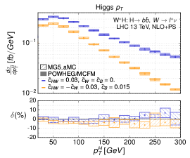
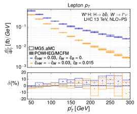
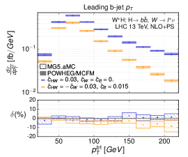
In Fig. 1, we present the transverse momentum spectrum of the system (upper left), of the leading (upper centre) and next-to-leading (upper right) -jets, of the lepton (middle left) and of the leading jet (middle centre). We then focus on the distribution in pseudorapidity for the system (middle right), in the transverse mass of the -boson and Higgs boson (lower left) and of the -boson, Higgs boson and leading-jet system (lower centre) and in the total transverse energy (lower right). In each subfigure, the results are shown both at the LO+PS and NLO+PS accuracies, together with uncertainties related to scale variation.
For each studied observable, we investigate in the first two lower bands of each subfigure the relative difference between the predictions in the SM and in the case of both considered benchmark points A and B,
| (18) |
In the last band, we additionally show differential -factors defined as the binned ratio of NLO to LO predictions taking only the total NLO uncertainty into account.
The predictions are found to be stable under radiative corrections, as expected for any process with a Drell–Yan-like topology. The obtained -factors are indeed relatively flat and independent of the EFT parameters, with the exception of the observables that rely on the leading-jet kinematics which turn out to be much harder at NLO. Hard QCD radiation contributions originating from the matrix element are in this case included, in contrast to the LO setup where QCD radiation is only described by the parton shower and thus modelled in the soft-collinear kinematical limit.
LO predictions are found to be inaccurate and do not overlap with the NLO results even after considering scale variation uncertainties. This is particularly true at high transverse momentum , transverse mass and total transverse energy . This behaviour is once again expected for a Drell–Yan-like process that does not depend on at fixed LO. If one were to use the difference between the LO and NLO results as an error estimate for the LO predictions and the scale variation only for the NLO, then the reduction of the theory error would be better reflected by Fig. 1. The ratios also remain stable with respect to QCD corrections, except at very high energies for the benchmark point A where small differences appear between the LO and NLO predictions. These would, by construction, be covered by the aforementioned improved definition of the LO theoretical uncertainties.
All distributions strongly depend on the value of the EFT Wilson coefficients. For the adopted scenario A, large enhancements are observed in the tails of the , and distributions, which correspond to a centrally produced system (with a small pseudorapidity). In contrast, event rates are only rescaled by about 15–20% with respect to the SM for the scenario B. This originates from the coupling that vanishes in this scenario, so that only the coupling drives the EFT behaviour in the high-energy tails. However, this latter coupling is known to yield a smaller impact than the coupling Maltoni:2013sma ; Mimasu:2015nqa , and it is therefore the presence of the interaction vertex in scenario A that leads to the large observed deviations. This constitutes a very promising avenue for setting limits on EFT parameters from studies and similar behaviour can be observed for production, where the and coefficients additionally play a role. In this case, the gluon fusion initiated contribution should however also be considered, as discussed in Refs. Mimasu:2015nqa ; Bylund:2016phk .
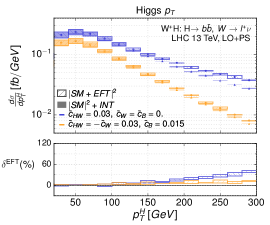
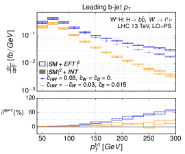
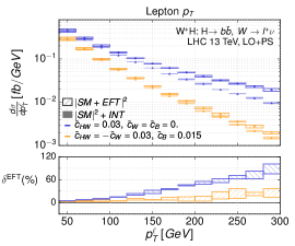
While such large enhancements can be exploited to obtain powerful constraints on the SMEFT Wilson coefficients, they do raise the question of the validity of the EFT approach at large momentum transfer Ellis:2014dva ; Biekoetter:2014jwa ; Englert:2014cva ; Contino:2016jqw . This question could be addressed with the use of dedicated benchmark models to compare the breakdown of the EFT framework against well-motivated ultraviolet-complete models Gorbahn:2015gxa ; Brehmer:2015rna . At a more simplistic level we can also make use of the MG5_aMC ability to select only interference contributions (at LO) to assess the impact of the squared EFT terms given our benchmark choices (technical details are described in Appendix A). Fig. 2 shows a selection of distributions, overlaying predictions with and without this squared term. We observe significant differences between the two choices that are greater than the scale uncertainty of the predictions. Depending on the observable, these can range from 40 to 100% on the interference-only prediction for the benchmark scenario A, while they are much milder for the benchmark scenario B. This suggests that current sensitivities on this region of the Wilson coefficient parameter space may not yet lend themselves to an EFT interpretation within the validity of the framework. A reduction of the production rate from the SM value, as seen for benchmark scenario B, moreover indicates the dominance of the interference term between the SM and EFT contributions given that the squared terms are positive-definite (Fig. 4).
5 Higgs production via vector boson fusion
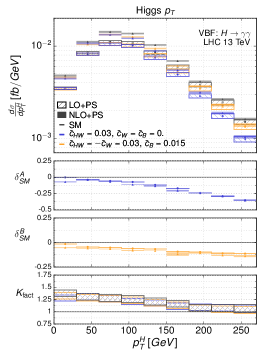
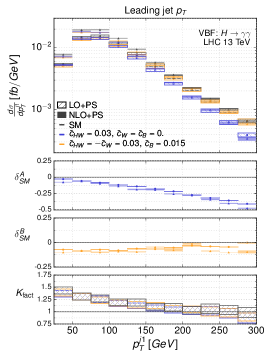
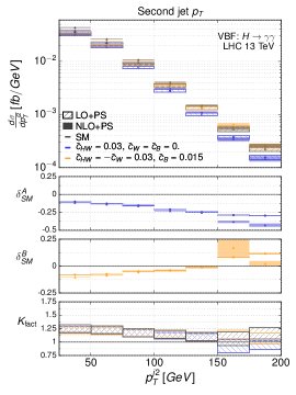
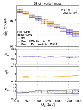
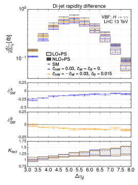
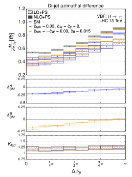
Another powerful probe of anomalous higher-derivative interactions between weak and Higgs bosons consists of the VBF Higgs production mode where it is produced in association with two forward jets,
| (19) |
Our event selection requires the presence of at least two jets with a pseudorapidity and a transverse momentum GeV, and we additionally impose the requirement that the Higgs boson decays into a pair of photons with a pseudorapidity satisfying and a transverse momentum GeV. We moreover include a standard VBF selection on the invariant mass and pseudorapidity separation of the pair of forward jets,
| (20) |
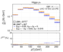
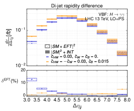
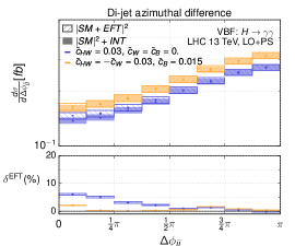
Several kinematical observables are sensitive to the momentum flow in the VBF process, for which EFT contributions deviate from the SM prediction. We consider in Fig. 4 the distribution in the transverse momentum of the diphoton system (upper left), in the of the leading (upper centre) and subleading (upper right) jets, in the invariant mass of the dijet system (lower left), as well as in its pseudorapidity (lower centre) and azimuthal angular (lower right) separations. The consistent definition of scale uncertainties that are possible with the NLO predictions helps to quantify the discriminatory power between the new physics benchmarks and the SM. Similarly to the VH process, the NLO corrections are independent of the EFT parameters and cannot be completely described by an overall -factor.
In contrast to the VH process, we observe a depletion of the production rate for both benchmark scenarios, which mainly impacts the high-energy tails of the differential distributions. This indicates that our predictions may be safer with respect to the validity of the EFT, as it implies that the interference term dominates over the EFT squared one. In particular, the effects for the benchmark scenario B are more pronounced with respect to the SM compared to the production case and show some different shape deformations. This illustrates the complementarity between the VH and VBF processes in disentangling the possible EFT sources for any potential deviation. Although the correlations between the forward jets as well as between the jets and the Higgs boson are known to be sensitive to new physics effects Englert:2012xt ; Djouadi:2013yb , those are less sensitive than the individual Higgs and jet distributions for our two benchmark scenarios.
We also repeat the simple EFT validity analysis performed for the case and assess the impact of the EFT squared terms at LO, as shown in Fig. 4. As suggested by the depletion effect of the EFT operators in the high energy bins of the differential distributions, the squared terms appear much more under control in this process compared to the case. Within the ranges of our predictions the impact of the squared term is again most pronounced for the benchmark A, reaching at most 5–12% while for benchmark B their effect is much smaller.
6 Future LHC reach
Before concluding, we attempt to estimate the reach of the LHC Run II with respect to the Wilson coefficients considered in our benchmark scenarios. Our results so far suggest to make use of the high energy tails of differential distributions as handles for new physics. For concreteness, we focus on the associated production process
which has already been searched for at both LHC Run I ATLAS-CONF-2013-079 and II ATLAS-CONF-2016-091 . In both analyses, a large number of signal and control regions are defined according to the lepton and additional jet multiplicities, as well as to the vector boson transverse momentum . These are combined in a global fit to obtain the corresponding SM Higgs signal strength. In this fitting procedure, several dominant components of the background, namely and -boson production in association with heavy-flavour jets, are left free to float. We consider as signal regions the overflow bin in the single lepton channel for both the zero-jet and one-jet categories. The Run II study, however makes use of multivariate methods in the event selection process that are difficult to reproduce – a task that definitely lies beyond the scope of the simple estimate we are intending to derive. We therefore choose to consider only the cut-based signal selection procedure employed in the Run I analysis and then project the results for various Run II integrated luminosities.
6.1 Signal prediction and background estimation
In order to estimate the number of background events in the single lepton signal regions of a possible cut-based, LHC Run II analysis, we extrapolate the results of the corresponding Run I analysis. We first consider the dominating contribution which arises from semi-leptonic top-antitop decays and which makes up 54 and 85% of the total background in the 0-jet and 1-jet categories, respectively. As a crude estimate for the corresponding 13 TeV yields, we compute a transfer factor (with , 1 for the 0-jet and 1-jet categories) by generating large statistics of SM semi-leptonic events at centre-of-mass energies of 8 and 13 TeV on which we apply the kinematic selection of the Run I analysis summarised in Appendix B. The transfer factor is defined as the ratio of the two fiducial cross sections and we deduce the Run II analysis background contributions by multiplying the 8 TeV SM expectation inferred from the Run I background event counts assuming 25 fb-1 of 8 TeV data. These should not depend much on the actual composition of 7 and 8 TeV data analysed, particularly in the high transverse momentum overflow bin which is dominated by 8 TeV data.
Table 4 summarises the information obtained and used in the subsequent analysis. Our theoretical predictions for the contributions to the 0- and 1-jet signal regions at 8 TeV, , lie within a factor 2 of the cross-sections inferred from the post-selection, fitted background decomposition presented in Table 5 of Ref. ATLAS-CONF-2013-079 . Due to the multi-variate nature of the recent Run II analysis, its fitted background yields cannot be used to validate the results of our projection, which rather represents the scenario in which a cut-based analysis similar to the Run I counterpart were performed at 13 TeV.
| Category(i) | ||||
|---|---|---|---|---|
| 0-jet | 74 | 0.94 fb | 3.92 fb | 4.17 |
| 1-jet | 143 | 3.20 fb | 8.05 fb | 2.52 |
The signal predictions have been generated using the previously described UFO implementation, and both the and contributions have been simulated at the NLO accuracy in QCD as described in previous sections, the fixed-order results being matched with Pythia 8 for both handling the top decays and the parton showering. A grid of points spanning the allowed region of the parameter space, including the SM prediction, was simulated and the generated events were passed through the same kinematic selection of Appendix B. Following the previous discussion on the existing constraints, we assume the simplification . Such a relation would not be retained in a complete global fit including, e.g., LEP data. However, it is instructive to follow this simplified path as it assesses the sensitivity of the LHC to the direction in the plane that is orthogonal, and thus complementary, to the one tightly constrained by precision measurements at the -pole. We have derived least-squares-fitted quadratic polynomial forms for the zero and one-jet overflow bin cross sections in the two-dimensional parameter plane . Our results, moreover, embed a -tagging efficiency of 70%, and more information (in particular on the explicit coefficients of the fits) is given in Appendix B.
6.2 Results
Our results have been derived from the fitted functional forms for the signal cross sections in combination with the projected background yields. We have performed a analysis to extract 95% confidence intervals assuming 30, 300 and 3000 fb-1 of integrated luminosities of 13 TeV proton-proton collisions. Denoting by and the event counts in the signal region in the background-only and signal-plus-background hypotheses, respectively, we have
| (21) |
The 95% confidence intervals are obtained at the boundary of which equates to the corresponding -value for a distribution with two degrees of freedom. Fig. 5 depicts these confidence intervals for the zero- and one-jet bin separately as well as their combination, for the three integrated luminosity points. For comparison, the marginalised single parameter exclusion regions established in Table 2 and the benchmark discussion of Sect. 2.3 are indicated.
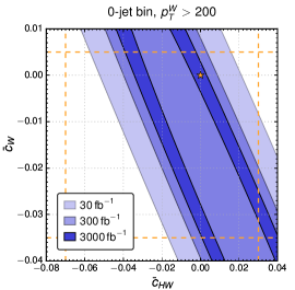
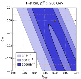
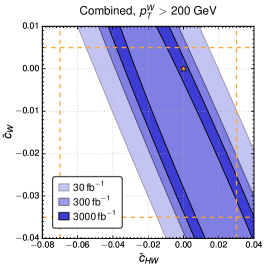
This simplified projection shows that this type of analysis is likely to substantially improve the existing limits on these Wilson coefficients in combination with existing data. Since the one-jet category suffers both from a larger background and smaller signal contribution, its relative impact on the overall reach is small. The blind direction associated with this measurement lies very close to the line, corresponding to the benchmark choice B of the earlier sections. This is consistent with the very mild expected impact of this particular new physics scenario in the high energy tails of the differential distributions for the process (see Sect. 4). Nevertheless, our results suggest that in the general case, taking the full integrated luminosity of LHC Run II will individually allow to constrain Wilson coefficients with a precision of a few per-mille and the results presented in Sec. 5 indicate that combining VBF and WH studies will break this degeneracy.
7 Conclusions
We have presented FeynRules and UFO implementations of dimension-six SMEFT operators affecting electroweak Higgs-boson production, which can be used for NLO(QCD)+PS accurate Monte Carlo event generation within the MG5_aMC framework. We have considered five SILH basis operators and have accounted for all field redefinitions that are necessary to canonically normalise the theory. Moreover, the ensuing modifications of both the gauge couplings and the relationships between the electroweak inputs and the derived parameters have also been included. We have showcased the strength of our approach by simulating both associated VH and VBF Higgs-boson production at the 13 TeV LHC, selecting a pair of benchmark scenarios informed both by recent limits from global fits to the LEP and LHC Run I data and by theoretical motivations originating from integrating out certain popular ultraviolet realisations.
We have found that EFT predictions and deviations from the SM are stable under higher-order corrections. Overall, we have also observed a significant reduction of the theoretical errors, which would have an impact on the future measurements aiming to unravel dimension-six operator contributions.
Furthermore, as a test for the validity of the EFT approach, we have proposed to compare distributions that either include the full matrix element (embedding all SM and new physics contributions) or account solely for the interference of the SM component with the new physics component. For our benchmark choices that saturate current experimental limits, the differences were observed to be large in the kinematic extremes of some of our distributions, particularly for production. This points to the possibility that the EFT description is breaking down in these regions of the parameter space and that the most precise measurements undertaken at the LHC Run II may be required to probe the EFT (while staying in its region of validity).
When comparing results for the VH and VBF channels, we have found that both Higgs-boson production modes are sensitive to new physics, but the VH one seems to have a better handle on -type () structure, since several key distributions display deviations that may be more easily distinguished from the background. Although the QCD -factors have been observed not to depend on the EFT parameters, the reduced theoretical uncertainties are crucial for disentangling a non-vanishing contribution of the -type structure to the predictions from the SM. This has been singled out in our study of the benchmark point B. Moreover, our results exhibit an interesting complementarity of the two Higgs production channels, since the interference pattern between the SM and the SMEFT contributions is quite different and benchmark-dependent.
In order to estimate the reach that might be possible at LHC Run II, we have performed a simplified analysis projecting the Run I SM background expectations in a search for associated production and combining this information with LHC Run II signal predictions obtained using our implementation. Using the overflow bin of the reconstructed -boson transverse momentum distribution in the single lepton channel as a probe for EFT effects suggests that the LHC Run II will significantly improve the current limits obtained from global fits. Clearly both the and VBF processes deserve further investigation including detector effects and an analysis strategy to reject the SM backgrounds. In this case, the new physics contributions to the SM background processes should also correctly be accounted for, since effective operators affecting electroweak Higgs-boson production also impact the normalisation of the triple gauge-boson interactions both directly and indirectly via the aforementioned field redefinitions Corbett:2013pja ; Ellis:2014jta ; Gorbahn:2015gxa ; Mimasu:2015nqa ; Butter:2016cvz .
Finally, our work has demonstrated a proof-of-concept for automated NLO+PS simulations in the SMEFT framework. To this aim, we have limited ourselves to a small set of dimension-six operators and a pair of benchmark points. This is characterised as a first step towards a complete operator basis implementation, in which the renormalisation group running of the Wilson coefficients Elias-Miro:2013gya ; Elias-Miro:2013mua ; Jenkins:2013zja ; Jenkins:2013wua ; Alonso:2013hga ; Maltoni:2016yxb could also be supplemented in the future.
Acknowledgements
We would like to express a special thanks to Fabio Maltoni for useful discussions. We moreover acknowledge the organisers of the 2015 ‘Les Houches–Physics at TeV colliders’ workshop and the Mainz Institute for Theoretical Physics for their hospitality and support during the completion of this work. CD is a Durham International Junior Research Fellow. BF and KMa have been supported by the Theory-LHC-France initiative of the CNRS (INP/IN2P3) and KMi and VS by the Science and Technology Facilities Council (Grant number ST/J000477/1).
Appendix A Simulation in MadGraph5_aMC@NLO
A.1 Technical details
Our HEL@NLO UFO model can be downloaded from the FeynRules model database FR-HEL:Online . It can be used for generating events at the NLO accuracy in QCD using software such as MG5_aMC via to the automated procedure detailed in Sect. 3. Event generation for production is achieved by typing in the MG5_aMC interpreter
   import model HELatNLO
   generate p p > h ve e+ [QCD]
   output
   launch
Since the usual decay syntax of MG5_aMC is not available for NLO event generation, we directly request the presence of the -boson decay products in the final state. An alternative way would require one to simulate the production of a Higgs boson in association with an on-shell -boson that is subsequently decayed within the MadSpin infrastructure Artoisenet:2012st ; Alwall:2014bza before invoking the parton showering. On the other hand, VBF Higgs-boson production is achieved by typing in the generation command
generate p p > h j j $$ w+ w- z a QCD=0 [QCD]
The removal of the -channel gauge boson contributions (via the $$ syntax) avoids the generation of VH topologies where the gauge boson decays hadronically.
In the parameter card, users may set values for the five Wilson coefficients defined in Eq. (5) as well as for the cutoff scale . The modifications to the electroweak parameters in terms of the inputs in the scheme are taken into account, as well as the shifts induced by the field redefinitions discussed in Sect. 2.
At the FeynRules level, the final Lagrangian involving all of the redefined fields and parameters is expanded up to . From the point at which this truncation occurs, all subsequent performed calculations will necessarily induce some (with ) dependence from, e.g., higher powers in the electroweak couplings. Furthermore, MG5_aMC constructs its matrix elements by squaring helicity amplitudes, so that the squared EFT contribution terms that are formally of are by default retained on top of the leading interference terms with the SM of . A positive definite cross section is ensured at the price of including higher-order terms. It is therefore important to remain in the regime where the EFT expansion can be trusted in that higher-order contributions are sufficiently suppressed. Departure from this safe zone may be reflected by a rapid growth of amplitudes with energy leading to extreme deviations in the tails of the distributions, as well as by discrepancies between independent Monte Carlo setups performing their truncation in different ways. Alternatively, this issue could be investigated thanks to some recent developments in MG5_aMC that allow the user to specify an order for the squared matrix element calculation, like QED^2 or QCD^2. However, this feature is currently only available for LO computations. For including the EFT effects in the simulation, the coupling order parameter NP can hence be set either to NP=1 to retain the full amplitude squared or to NP^2<=1 to throw away the aforementioned EFT squared terms, e.g.
generate p p > h ve e+ NP^2<=1
Finally, due to the details of the implementation, we advise users seeking to recover the SM limit to avoid setting the Wilson coefficients to zero. It is preferable to either set them to very small non-zero values or to use restrictions. The cutoff scale parameter NPl may also be alternatively fixed to a very large value.
A.2 Comparison with the MCFM/POWHEG-BOX implementation
We have verified that our results in the channel are compatible with those stemming from an alternative existing implementation, which is based on MCFM Campbell:1999ah ; Campbell:2011bn ; Campbell:2015qma and the Powheg-Box framework Frixione:2007vw ; Alioli:2010xd and that has been introduced in Ref. Mimasu:2015nqa . We have scrutinised several differential distributions for both our benchmark points in the Powheg and MG5_aMC frameworks, as presented in Fig. 6. A good consistency has been found up to statistical uncertainties and despite the difference in the dynamical scale choice which is taken as in MG5_aMC and the invariant mass of the Higgs-vector boson system in the Powheg-Box implementation.
Appendix B Fit to kinematic selection of ATLAS-CONF-2013-079
We summarise here the kinematic selection through which the and signal events have been passed in order to determine the background transfer factor and signal efficiencies of the analysis performed in Ref. ATLAS-CONF-2013-079 . The signal region used is the GeV overflow bin in the 0 and 1-jet categories of the single-lepton channel. The kinematic selection for this channel applied to our event samples after parton shower is as follows:
-
We require the final state to contain exactly one lepton with and GeV.
-
Jets reconstructed by means of the anti- jet algorithm with a radius parameter , and we discard the jet candidates for which the conditions and GeV are not satisfied.
-
We require exactly two -jets with a pseudorapidity , the hardest one being further imposed tho have a transverse momentum 45 GeV.
Not more than one additional jet in the region is allowed and any event with a jet with 30 GeV in the region is also rejected. Events are then split into the zero- and one-jet categories based on the presence of an extra, non-forward jet softer than the two -jets. The vector boson transverse momentum is defined as the vector sum of the transverse momentum of the lepton and the missing transverse energy. Additionally, in the overflow bin, a cut of 50 GeV on the missing energy is imposed as well as a cut on the distance between the two -jets, . A flat -tagging efficiency of 70% is in addition assumed.
34 signal samples have been simulated with the Wilson coefficients being taken in the ranges and , the total rates being rescaled by the Higgs branching fraction to obtained with eHDECAY. These events have then been passed through the above selection in order to determine the functional forms for the zero- and one-jet signal cross sections in overflow bin, and . A least-squares fit yields
| (22) | ||||
| (23) |
The fit coefficients are within 5–10% of one another, which is to be expected given that our signal process receives contributions from an electroweak vertex and should not be directly sensitive to additional QCD radiation.
References
- (1) B. Grzadkowski, M. Iskrzynski, M. Misiak, and J. Rosiek, Dimension-six terms in the standard model Lagrangian, JHEP 1010 (2010) 085, [arXiv:1008.4884].
- (2) R. Contino, M. Ghezzi, C. Grojean, M. Mühlleitner, and M. Spira, Effective Lagrangian for a light Higgs-like scalar, JHEP 1307 (2013) 035, [arXiv:1303.3876].
- (3) R. S. Gupta, A. Pomarol, and F. Riva, BSM primary effects, Phys. Rev. D91 (2015), no. 3 035001, [arXiv:1405.0181].
- (4) A. Falkowski, B. Fuks, K. Mawatari, K. Mimasu, F. Riva, and V. Sanz, Rosetta: an operator basis translator for standard model effective field theory, Eur. Phys. J. C75 (2015), no. 12 583, [arXiv:1508.05895].
- (5) LHC Higgs Cross Section Working Group Collaboration, D. de Florian et al., Handbook of LHC Higgs Cross Sections: 4. Deciphering the Nature of the Higgs Sector, [arXiv:1610.07922].
- (6) S. Frixione and B. R. Webber, Matching NLO QCD computations and parton shower simulations, JHEP 06 (2002) 029, [hep-ph/0204244].
- (7) O. Latunde-Dada, MC and NLO for the hadronic decay of Higgs bosons in associated production with vector bosons, JHEP 05 (2009) 112, [arXiv:0903.4135].
- (8) S. Frixione, P. Torrielli, and M. Zaro, Higgs production through vector-boson fusion at the NLO matched with parton showers, Phys. Lett. B726 (2013) 273–282, [arXiv:1304.7927].
- (9) P. Nason, A new method for combining NLO QCD with shower Monte Carlo algorithms, JHEP 11 (2004) 040, [hep-ph/0409146].
- (10) K. Hamilton, P. Richardson, and J. Tully, A positive-weight next-to-leading order Monte Carlo simulation for Higgs boson production, JHEP 04 (2009) 116, [arXiv:0903.4345].
- (11) P. Nason and C. Oleari, NLO Higgs boson production via vector-boson fusion matched with shower in POWHEG, JHEP 02 (2010) 037, [arXiv:0911.5299].
- (12) G. Luisoni, P. Nason, C. Oleari, and F. Tramontano, /HZ + 0 and 1 jet at NLO with the POWHEG BOX interfaced to GoSam and their merging within MiNLO, JHEP 10 (2013) 083, [arXiv:1306.2542].
- (13) D. Goncalves, F. Krauss, S. Kuttimalai, and P. Maierhöfer, Higgs-Strahlung: merging the NLO Drell-Yan and loop-induced 0+1 jet multiplicities, Phys. Rev. D92 (2015), no. 7 073006, [arXiv:1509.01597].
- (14) F. Campanario, R. Roth, and D. Zeppenfeld, QCD radiation in and production and anomalous coupling measurements, Phys. Rev. D91 (2015) 054039, [arXiv:1410.4840].
- (15) V. Hankele, G. Klamke, D. Zeppenfeld, and T. Figy, Anomalous Higgs boson couplings in vector boson fusion at the CERN LHC, Phys. Rev. D74 (2006) 095001, [hep-ph/0609075].
- (16) P. Artoisenet, P. de Aquino, F. Demartin, R. Frederix, S. Frixione, et al., A framework for Higgs characterisation, JHEP 1311 (2013) 043, [arXiv:1306.6464].
- (17) F. Maltoni, K. Mawatari, and M. Zaro, Higgs characterisation via vector-boson fusion and associated production: NLO and parton-shower effects, Eur. Phys. J. C74 (2014), no. 1 2710, [arXiv:1311.1829].
- (18) A. Denner, S. Dittmaier, S. Kallweit, and A. Muck, Electroweak corrections to Higgs-strahlung off W/Z bosons at the Tevatron and the LHC with HAWK, JHEP 03 (2012) 075, [arXiv:1112.5142].
- (19) M. C. Kumar, M. K. Mandal, and V. Ravindran, Associated production of Higgs boson with vector boson at threshold N3LO in QCD, JHEP 03 (2015) 037, [arXiv:1412.3357].
- (20) J. M. Campbell, R. K. Ellis, and C. Williams, Associated production of a Higgs boson at NNLO, JHEP 06 (2016) 179, [arXiv:1601.00658].
- (21) F. A. Dreyer and A. Karlberg, Vector-boson fusion Higgs production at three loops in QCD, Phys. Rev. Lett. 117 (2016), no. 7 072001, [arXiv:1606.00840].
- (22) M. Cacciari, F. A. Dreyer, A. Karlberg, G. P. Salam, and G. Zanderighi, Fully differential vector-boson-fusion Higgs production at next-to-next-to-leading order, Phys. Rev. Lett. 115 (2015), no. 8 082002, [arXiv:1506.02660].
- (23) K. Mimasu, V. Sanz, and C. Williams, Higher order QCD predictions for associated Higgs production with anomalous couplings to gauge bosons, JHEP 08 (2016) 039, [arXiv:1512.02572].
- (24) A. Alloul, N. D. Christensen, C. Degrande, C. Duhr, and B. Fuks, FeynRules 2.0 - A complete toolbox for tree-level phenomenology, Comput. Phys. Commun. 185 (2014) 2250–2300, [arXiv:1310.1921].
- (25) C. Degrande, Automatic evaluation of UV and R2 terms for beyond the standard model Lagrangians: a proof-of-principle, Comput. Phys. Commun. 197 (2015) 239–262, [arXiv:1406.3030].
- (26) J. Alwall, R. Frederix, S. Frixione, V. Hirschi, F. Maltoni, O. Mattelaer, H. S. Shao, T. Stelzer, P. Torrielli, and M. Zaro, The automated computation of tree-level and next-to-leading order differential cross sections, and their matching to parton shower simulations, JHEP 07 (2014) 079, [arXiv:1405.0301].
- (27) http://feynrules.irmp.ucl.ac.be/wiki/HELatNLO.
- (28) N. D. Christensen, P. de Aquino, C. Degrande, C. Duhr, B. Fuks, M. Herquet, F. Maltoni, and S. Schumann, A Comprehensive approach to new physics simulations, Eur. Phys. J. C71 (2011) 1541, [arXiv:0906.2474].
- (29) C. Degrande, C. Duhr, B. Fuks, D. Grellscheid, O. Mattelaer, and T. Reiter, UFO - the universal FeynRules output, Comput. Phys. Commun. 183 (2012) 1201–1214, [arXiv:1108.2040].
- (30) P. de Aquino, W. Link, F. Maltoni, O. Mattelaer, and T. Stelzer, ALOHA: automatic libraries of helicity amplitudes for Feynman diagram computations, Comput. Phys. Commun. 183 (2012) 2254–2263, [arXiv:1108.2041].
- (31) F. Maltoni, E. Vryonidou, and C. Zhang, Higgs production in association with a top-antitop pair in the standard model Effective Field Theory at NLO in QCD, JHEP 10 (2016) 123, [arXiv:1607.05330].
- (32) C. Burges and H. J. Schnitzer, Virtual effects of excited quarks as probes of a possible new hadronic mass scale, Nucl.Phys. B228 (1983) 464.
- (33) C. N. Leung, S. Love, and S. Rao, Low-energy manifestations of a new interaction scale: operator analysis, Z.Phys. C31 (1986) 433.
- (34) W. Buchmuller and D. Wyler, Effective Lagrangian analysis of new interactions and flavor conservation, Nucl.Phys. B268 (1986) 621.
- (35) S.-F. Ge, H.-J. He, and R.-Q. Xiao, Probing new physics scales from Higgs and electroweak observables at e+ e− Higgs factory, JHEP 10 (2016) 007, [arXiv:1603.03385].
- (36) G. Giudice, C. Grojean, A. Pomarol, and R. Rattazzi, The strongly-interacting light Higgs, JHEP 0706 (2007) 045, [hep-ph/0703164].
- (37) A. Alloul, B. Fuks, and V. Sanz, Phenomenology of the Higgs effective lagrangian via FEYNRULES, JHEP 1404 (2014) 110, [arXiv:1310.5150].
- (38) J. Ellis, V. Sanz, and T. You, The effective standard model after LHC run I, JHEP 03 (2015) 157, [arXiv:1410.7703].
- (39) J. Ellis, V. Sanz, and T. You, Complete Higgs sector constraints on dimension-6 operators, JHEP 07 (2014) 036, [arXiv:1404.3667].
- (40) ATLAS Collaboration, G. Aad et al., Constraints on non-standard model Higgs boson interactions in an effective Lagrangian using differential cross sections measured in the decay channel at TeV with the ATLAS detector, Phys. Lett. B753 (2016) 69–85, [arXiv:1508.02507].
- (41) M. Gorbahn, J. M. No, and V. Sanz, Benchmarks for Higgs effective theory: extended Higgs sectors, JHEP 10 (2015) 036, [arXiv:1502.07352].
- (42) T. Hahn, Generating Feynman diagrams and amplitudes with FeynArts 3, Comput. Phys. Commun. 140 (2001) 418–431, [hep-ph/0012260].
- (43) V. Hirschi, R. Frederix, S. Frixione, M. V. Garzelli, F. Maltoni, and R. Pittau, Automation of one-loop QCD corrections, JHEP 05 (2011) 044, [arXiv:1103.0621].
- (44) S. Frixione, Z. Kunszt, and A. Signer, Three jet cross-sections to next-to-leading order, Nucl. Phys. B467 (1996) 399–442, [hep-ph/9512328].
- (45) R. Frederix, S. Frixione, F. Maltoni, and T. Stelzer, Automation of next-to-leading order computations in QCD: the FKS subtraction, JHEP 10 (2009) 003, [arXiv:0908.4272].
- (46) NNPDF Collaboration, R. D. Ball, V. Bertone, S. Carrazza, L. Del Debbio, S. Forte, A. Guffanti, N. P. Hartland, and J. Rojo, Parton distributions with QED corrections, Nucl. Phys. B877 (2013) 290–320, [arXiv:1308.0598].
- (47) T. Sjostrand, S. Mrenna, and P. Z. Skands, A brief introduction to PYTHIA 8.1, Comput. Phys. Commun. 178 (2008) 852–867, [arXiv:0710.3820].
- (48) R. Contino, M. Ghezzi, C. Grojean, M. Mühlleitner, and M. Spira, ehdecay: an implementation of the higgs effective lagrangian into hdecay, Comput.Phys.Commun. 185 (2014) 3412–3423, [arXiv:1403.3381].
- (49) E. Conte, B. Fuks, and G. Serret, MadAnalysis 5, a user-friendly framework for collider phenomenology, Comput.Phys.Commun. 184 (2013) 222–256, [arXiv:1206.1599].
- (50) M. Cacciari, G. P. Salam, and G. Soyez, FastJet user manual, Eur. Phys. J. C72 (2012) 1896, [arXiv:1111.6097].
- (51) M. Cacciari, G. P. Salam, and G. Soyez, The anti-k(t) jet clustering algorithm, JHEP 04 (2008) 063, [arXiv:0802.1189].
- (52) R. Frederix, S. Frixione, V. Hirschi, F. Maltoni, R. Pittau, and P. Torrielli, Four-lepton production at hadron colliders: aMC@NLO predictions with theoretical uncertainties, JHEP 02 (2012) 099, [arXiv:1110.4738].
- (53) J. Ellis, D. S. Hwang, V. Sanz, and T. You, A fast track towards the ‘Higgs’ spin and parity, JHEP 11 (2012) 134, [arXiv:1208.6002].
- (54) O. Bessidskaia Bylund, F. Maltoni, I. Tsinikos, E. Vryonidou, and C. Zhang, Probing top quark neutral couplings in the standard model effective field theory at NLO in QCD, JHEP 05 (2016) 052, [arXiv:1601.08193].
- (55) A. Biekötter, A. Knochel, M. Krämer, D. Liu, and F. Riva, Vices and virtues of Higgs effective field theories at large energy, Phys. Rev. D91 (2015) 055029, [arXiv:1406.7320].
- (56) C. Englert and M. Spannowsky, Effective theories and measurements at colliders, Phys. Lett. B740 (2015) 8–15, [arXiv:1408.5147].
- (57) R. Contino, A. Falkowski, F. Goertz, C. Grojean, and F. Riva, On the validity of the effective field theory approach to sm precision tests, JHEP 07 (2016) 144, [arXiv:1604.06444].
- (58) J. Brehmer, A. Freitas, D. Lopez-Val, and T. Plehn, Pushing Higgs effective theory to its limits, Phys. Rev. D93 (2016), no. 7 075014, [arXiv:1510.03443].
- (59) C. Englert, D. Goncalves-Netto, K. Mawatari, and T. Plehn, Higgs quantum numbers in weak boson fusion, JHEP 01 (2013) 148, [arXiv:1212.0843].
- (60) A. Djouadi, R. M. Godbole, B. Mellado, and K. Mohan, Probing the spin-parity of the Higgs boson via jet kinematics in vector boson fusion, Phys. Lett. B723 (2013) 307–313, [arXiv:1301.4965].
- (61) ATLAS Collaboration, Search for the bb decay of the standard model Higgs boson in associated W/ZH production with the ATLAS detector, Tech. Rep. ATLAS-CONF-2013-079, CERN, Geneva, (2013).
- (62) ATLAS Collaboration, Search for the standard model Higgs boson produced in association with a vector boson and decaying to a pair in collisions at 13 TeV using the ATLAS detector, Tech. Rep. ATLAS-CONF-2016-091, CERN, Geneva, (2016).
- (63) T. Corbett, O. J. P. Éboli, J. Gonzalez-Fraile, and M. C. Gonzalez-Garcia, Determining triple gauge boson couplings from Higgs data, Phys. Rev. Lett. 111 (2013) 011801, [arXiv:1304.1151].
- (64) A. Butter, O. J. P. Éboli, J. Gonzalez-Fraile, M. C. Gonzalez-Garcia, T. Plehn, and M. Rauch, The gauge-Higgs legacy of the LHC run I, JHEP 07 (2016) 152, [arXiv:1604.03105].
- (65) J. Elias-Miró, J. R. Espinosa, E. Massó, and A. Pomarol, Renormalization of dimension-six operators relevant for the Higgs decays , JHEP 08 (2013) 033, [arXiv:1302.5661].
- (66) J. Elias-Miro, J. R. Espinosa, E. Massó, and A. Pomarol, Higgs windows to new physics through d=6 operators: constraints and one-loop anomalous dimensions, JHEP 11 (2013) 066, [arXiv:1308.1879].
- (67) E. E. Jenkins, A. V. Manohar, and M. Trott, Renormalization group evolution of the standard model dimension six operators I: formalism and lambda dependence, JHEP 10 (2013) 087, [arXiv:1308.2627].
- (68) E. E. Jenkins, A. V. Manohar, and M. Trott, Renormalization group evolution of the standard model dimension six operators II: Yukawa dependence, JHEP 01 (2014) 035, [arXiv:1310.4838].
- (69) R. Alonso, E. E. Jenkins, A. V. Manohar, and M. Trott, Renormalization group evolution of the standard model dimension six operators III: gauge coupling dependence and phenomenology, JHEP 04 (2014) 159, [arXiv:1312.2014].
- (70) P. Artoisenet, R. Frederix, O. Mattelaer, and R. Rietkerk, Automatic spin-entangled decays of heavy resonances in Monte Carlo simulations, JHEP 03 (2013) 015, [arXiv:1212.3460].
- (71) J. Alwall, C. Duhr, B. Fuks, O. Mattelaer, D. G. Ozturk, and C.-H. Shen, Computing decay rates for new physics theories with FeynRules and MadGraph5_aMC@NLO, Comput. Phys. Commun. 197 (2015) 312–323, [arXiv:1402.1178].
- (72) J. M. Campbell and R. K. Ellis, An update on vector boson pair production at hadron colliders, Phys. Rev. D60 (1999) 113006, [hep-ph/9905386].
- (73) J. M. Campbell, R. K. Ellis, and C. Williams, Vector boson pair production at the LHC, JHEP 07 (2011) 018, [arXiv:1105.0020].
- (74) J. M. Campbell, R. K. Ellis, and W. T. Giele, A multi-threaded version of MCFM, Eur. Phys. J. C75 (2015), no. 6 246, [arXiv:1503.06182].
- (75) S. Frixione, P. Nason, and C. Oleari, Matching NLO QCD computations with parton shower simulations: the POWHEG method, JHEP 11 (2007) 070, [arXiv:0709.2092].
- (76) S. Alioli, P. Nason, C. Oleari, and E. Re, A general framework for implementing NLO calculations in shower Monte Carlo programs: the POWHEG BOX, JHEP 06 (2010) 043, [arXiv:1002.2581].