Belt(s) of debris resolved around the Sco-Cen star HIP 67497^,

Abstract

Aims. In 2015, we initiated a survey of Scorpius-Centaurus A-F stars that are predicted to host warm-inner and cold-outer belts of debris similar to the case of the system HR 8799. The survey aims to resolve the disks and detect planets responsible for the disk morphology. In this paper, we study the F-type star HIP 67497 and present a first-order modelisation of the disk in order to derive its main properties.

Methods. We used the near-infrared integral field spectrograph (IFS) and dual-band imager IRDIS of VLT/SPHERE to obtain angular-differential imaging observations of the circumstellar environnement of HIP 67497. We removed the stellar halo with PCA and TLOCI algorithms. We modeled the disk emission with the GRaTeR code.

Results. We resolve a ring-like structure that extends up to $\sim$450 mas ($\sim$50 au) from the star in the IRDIS and IFS data. It is best reproduced by models of a non-eccentric ring with an inclination of $80\pm 1^{\circ}$, a position angle of $-93\pm 1^{\circ}$, and a semi-major axis of $59\pm 3$ au. We also detect an additional, but fainter, arc-like structure with a larger extension (0.65 arcsec) South of the ring that we model as a second belt of debris at $\sim$130 au. We detect 10 candidate companions at separations $\geq$1”. We estimate the mass of putative perturbers responsible for the disk morphology and compare it to our detection limits. Additional data are needed to find those perturbers, and to relate our images to large-scale structures seen with HST/STIS.

1 Introduction

The Scorpius-Centaurus OB association (Sco-Cen) is the nearest site of recent massive star formation (de Zeeuw et al. 1999). The proximity (d=90-200 pc) and young age ($\sim$11-17 Myr) of Sco-Cen all contribute to make it an excellent niche for direct imaging (DI) search of planets and disks. The planet imager instruments GPI (Macintosh & Graham, J. R., et al. 2008) and SPHERE (Beuzit et al. 2008) have initiated surveys of the circumstellar environment of a few Sco-Cen stars at unprecedented contrasts and angular resolution. They have already resolved several new debris disks around those stars (Currie et al. 2015; Kasper et al. 2015; Kalas et al. 2015; Lagrange et al. 2016; Draper et al. 2016) with wing-tilt and ringed morphologies indicative of the presence of planets.

We initiated a DI survey with SPHERE to image new giant planets and circumstellar disks around a sample of Sco-Cen F5-A0 stars with infrared excess. The excesses can be modeled by 2 black-body components, each corresponding to a belt of debris (Chen et al. 2014, hereafter C14). This architecture is reminiscent of the Solar System, and of benchmark systems previously identified by DI like HR 8799 (Marois et al. 2008, 2010), or HD 95086 (Rameau et al. 2013) which is also part of Sco-Cen.
In the course of the survey, we resolved a disk around the F0-type star HIP 67497 (HD 120326). This intermediate-mass star (M$=1.6M_{\odot}$) is located at a distance of $107.4^{+10.4}_{-8.7}$ pc (van Leeuwen 2007) and belongs to the 16 Myr old (Mamajek et al. 2002) Upper Centaurus Lupus sub-group (de Zeeuw et al. 1999). C14 modeled the infrared excess of the star with two belts of debris: a cold ($127\pm 5$ K) bright ($L_{IR}/L_{*}=1.1\times 10^{-3}$) belt at 13.9 au and a second colder ($63\pm 5$ K) dimmer ($L_{IR}/L_{*}=1.4\times 10^{-4}$) belt at 116.5 au. The same team produced an alternative model of the excess requiring only one belt located at 8.82$\pm$1 au (Jang-Condell et al. 2015). Previous observations with adaptive optics systems did not reveal any companion or structure close to HIP 67497 (Janson et al. 2013). Our resolved observations therefore offer the opportunity to better constrain the radial distribution of the dust around this star and to look for the companions responsible for that distribution.

We present the observations and data in § 2, and the models in § 3. We discuss the morphology of the disk and the existence of putative perturbers (planets) in § 4.

2 Observations and data reduction

Table 1: Log of observations, April 6, 2016.

		IRDIS	IFS
UT time	Neutral density	$\mathrm{DIT\times NDIT\times N_{EXP}}$		$\Delta$PA	$<$Seeing$>$	Airmass	$\tau_{0}$	Remarks
HH:MM		(s)	(s)	(∘)	(”)		(ms)
04:49	ND_1.0	4$\times$2$\times$1	8$\times$1$\times$1	0.1	1.2	1.1	3.7	Unsat. PSF
04:50	ND_0.0	32$\times$1$\times$1	64$\times$1$\times$1	0.1	1.2	1.1	4.6	Star center
04:50	ND_0.0	32$\times$8$\times$16	64$\times$4$\times$16	37.5	1.1	1.1	3.5	ADI sequence
06:01	ND_1.0	4$\times$2$\times$1	8$\times$1$\times$1	0.1	1.1	1.1	2.9	Unsat. PSF
06:02	ND_0.0	32$\times$1$\times$1	64$\times$1$\times$1	0.1	1.0	1.1	3.0	Star center

We observed HIP 67497 on April 6, 2016 with the VLT/SPHERE instrument (Beuzit et al. 2008) operated in IRDIFS mode (Tab. 1). The mode enables for pupil-stabilized observations of the source placed behind an apodized Lyot coronagraph (92.5 mas radius) with the IRDIS (Dohlen et al. 2008) and IFS (Claudi et al. 2008) sub-instruments operated in parallel. IRDIS yielded images of $\sim$11.1$\times$12.4” centered onto the star in the H2 ($\lambda_{c}$=1.593$\mu$m, width=52 nm) and H3 ($\lambda_{c}$=1.667$\mu$m, width=54 nm) filters (Vigan et al. 2010). The IFS datacubes are made of 39 images covering the 0.96-1.33$\mu$m spectral range and a square field-of-view of 1.8 arcseconds. For registration purposes — for both sub-instruments before and after the deep exposures — we obtained frames with satellite spots (Star Center) created by a waffle pattern introduced onto the deformable mirror of the instrument. Those frames were used to assess the position of the star behind the coronagraphic mask. We recorded additional non-saturated exposures of the star placed outside of the coronagraphic mask with the neutral density filter ND_1.0 to estimate the flux and position of point sources.

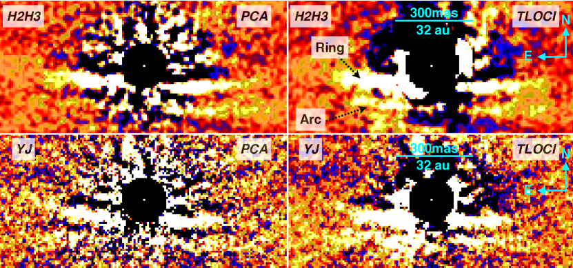
Figure 1: Images of the disk structure around HIP 67497 obtained with the IFS (YJ), and IRDIS (H2H3), and considering PCA and TLOCI reductions.

We reduced the IRDIS data with the Data Reduction Handling software (DRH) of SPHERE (Pavlov et al. 2008). The DRH corrected the raw science frames from the bad pixels, subtracted the dark, and recentered the images onto a common origin using the Star Center images. The field rotation of 37.5^∘ during the sequence of coronagraphic exposures was sufficient to apply the angular differential imaging (ADI) technique and reveal point sources down to 0.1”. We applied a Principal Component Analysis (PCA) algorithm (Soummer et al. 2012) on the H2 and H3 images separately to attenuate the stellar halo. The small number of modes kept in the PCA (10) enabled to look for extended structures. We used the TLOCI algorithm (Marois et al. 2014) to identify point sources and to confirm the structures.

The IFS data were analysed with a custom pipeline (Vigan et al. 2015, hereafter V15). This tool subtracted the background, interpolated the bad pixels, removed the instrument crosstalk, and performed a wavelength calibration of the spectra on the 2D raw frames. The DRH was then used to build the cubes from the 2D calibrated frames. We performed a PCA taking advantage of the wavelength coverage and field rotation to look for point sources (V15). We also performed PCA and TLOCI reductions of the IFS data after collapsing each cube in wavelength in order to reveal the (extended, faint) disk structures.

We used the True North value of $-1.649\pm 0.019^{\circ}$, and platescales of $12.257\pm 0.004$ and $7.46\pm 0.02$ mas/pixel for IRDIS and the IFS, respectively. These values are derived from the observations of the NGC3603 astrometric field obtained as part of the SPHERE GTO survey on March 30, 2016 (priv. com.).

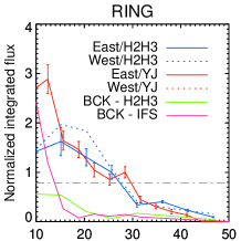
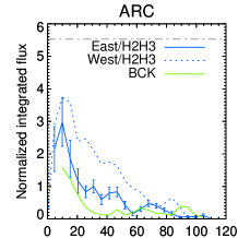
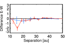
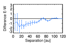
Figure 2: Radial profile along the disk position angle for the ring (left) and for the arc (right), extracted from the H2H3, and YJ PCA images and normalized to the median emission of the east side from 15 to 40 au. The residuals between the East and West disk profiles are shown at bottom. The normalization is different for the right and left panels. The dot-dashed line correspond to the cut of Fig. 1

3 Disk properties

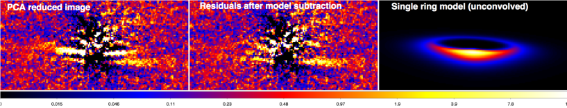
Figure 3: Results of the forward modeling for the case of a single belt. Left: PCA image of the disk. Middle: Residuals after subtraction of the best single ring model, with the same linear color scale as the left image. Right: best single ring model (unconvolved with the SPHERE PSF) in a log scale to show the fainter backward side of the disk.

We detect an inclined ring at the same position in our collapsed YJ, H2, and H3 images (Fig. 1). The ring structure is seen both in our PCA and TLOCI reductions. It is also retrieved when exploiting both the ADI technique and the wavelength diversity of the IFS and IRDIS (ASDI). We are confident this is a real structure, not related to the stellar halo. The ring extends up to 450 mas, or 50 au, from the star in the IRDIS images. It has a smaller apparent extension (40 au) in the YJ images. This is likely due to the lower S/N of those data. We derived the flux profile (non corrected from artifacts introduced by the ADI; Milli et al. 2012) along the position angle of the ring from the H2H3, and YJ PCA images (Fig. 2). To improve the S/N, we averaged the flux over circular apertures of one FWHM diameter centered on that axis. The error bars for the East and West sides are computed from the dispersion of the flux within each aperture. They are of comparable amplitude. We also report the flux profile of the residual background (”BCK”) extracted along the same appertures but tilted at a position angle perpandicular to the disk one (green and pink lines). The profiles indicate that the ring is rougthly symmetric and has a similar flux profile in the YJ and H2/H3 bands from 15 to 50 au. Below 15 au and down to the coronagraph (10 au), the flux profile can be affected by residual speckles.

An additional arc-like structure (”Arc” in Fig. 1) is detected at 40 mas South of the main ring. It extends visually up to 650 mas on the west side (70 au). This arc structure shows a strong flux asymmetry compared to the ring (Fig. 2). It is also retrieved at the same position into the IFS and IRDIS image for both TLOCI and PCA reductions. As for the ring, we are confident this feature is real and not a residual from the stellar halo. In the following section, we attempt a first characterization of the observed structures to better understand their nature. A more detailed modeling will be done in a forthcoming study.

3.1 Model

We injected scattered light disk models into the IRDIS data to interpret the observed features. The disk models were generated with the GRaTeR code (Augereau et al. 1999). GRaTeR considers a power-law for the radial distribution of the dust of index $\alpha_{\text{in}}>0$ and $\alpha_{\text{out}}<0$ inward and outward of a reference radius $r_{0}(\theta)$ respectively. The disk model is rotated to the angles of the initial frames, convolved with the measured PSF and then subtracted from the data. The resulting images are re-reduced using the PCA algorithm used for the data reduction to obtain a disc-subtracted image. This step is repeated iteratively by varying the free parameters of the disk model until a reduced $\chi^{2}$ computed in the part of the model-subtracted image in a zone covering the location of the disk on the averaged H2+H3 images is minimized.

We assumed a grey color for the disk between H2 and H3. To limit the parameter space, we adopted a distribution of optically thin dust with constant effective scattering cross-section.

3.2 Inner ring

To model the inner ring, we fixed the inner and outer slope to $\alpha_{\text{in}}=10$ and $\alpha_{\text{out}}=-5$ to mimic sharp edges. We assumed a circular ring, with anisotropic scattering parametrized by a Henyey-Greenstein parameter g. Therefore, the model has five free parameters (semi-major axis $r_{0}$, position angle PA, inclination $i_{tilt}$, g, and the flux). The $\chi^{2}$ (hereafter $\chi^{2}_{\text{region\>1}}$) is computed in a region encompassing only the inner belt (see App. A). The parameters of the best-fitting model are reported in Tab. 2 and details on the minimization are given in App. A. The initial PCA-reduced image, best model and PCA-reduced image after best model subtraction are shown in Fig. 3.

The ”arc” structure is still present in the residual image (Fig. 3), thus indicating that it is not a product of self-subtraction effects from the ring. We compare two possible models of that structure in the following section.

Table 2: Morphology of the inner belt

PA (∘)	$r_{0}$ (au)	$i_{tilt}$ (∘)	g	$\chi^{2}_{\text{region\>1}}$
-93$\pm 1$	$58.6\pm 3$	$80\pm 1$	0.82$\pm 0.02$	2.6

3.3 Model of the arc

We considered the best model of the inner ring (§ 3.2) and modeled the arc with a second, outer belt. We assumed the same inclination, position angle and g parameter as for the inner belt. The outer slope $\alpha_{\text{out}}$, the radius and the flux ratio with respect to the inner belt are left as free parameters. The $\chi^{2}$ (hereafter $\chi^{2}_{\text{region\>2}}$) is now computed on a region encompassing the pixels where the ring and the arc are detected (App. A).

As an alternative, we investigated whether a narrow belt and a smooth disk halo could reproduce the ring and the arc. We did so by analogy with HR 8799 where such a halo was proposed (Su et al. 2009). We used for the ring the best fit found in §  3.2, and added a smooth halo modeled by an additional disk of outer slope $\alpha_{\text{out,halo}}<\alpha_{\text{out}}$ and with a flux scaling factor lower than that of the narrow belt. In total, there are 3 free parameters: $\alpha_{\text{out,halo}}$, the narrow belt flux, and the halo flux.

Table 3: Results of the modeling of the belt and arc

Model	$\alpha_{\text{out}}$	$r_{0}$ (au)	flux ratio	$\chi^{2}_{\text{region\>2}}$
Two belts	-8${}^{+4}_{-8}$	130$\pm 8$	0.08$\pm 0.03$	3.5
Belt+halo	-1.3${}^{+0.6}_{-0.8}$	n.a.	0.66$\pm$0.40	3.8

The best fit parameters are given in Tab. 3 and the residuals after subtraction of the two models are shown in Fig. 4. The residuals are slightly higher for the case of the ring+halo model. The scenario including two belts of debris is favored by the present data.

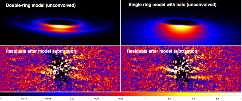
Figure 4: Results of the forward modeling for the case of two belts (left panels, reduced $\chi^{2}=3.5$) and a narrow-ring laid over a smooth halo (right, reduced $\chi^{2}=3.8$). The models are shown on top and the post-ADI residual images at the bottom.

4 Concluding remarks

The disk around HIP 67497 has an infrared luminosity (IL) in the same range as the disks already resolved around the Sco-Cen A-F type stars HD 111520, HIP 79977, HD 106906, and HD 115600 ($L_{IR}/L_{*}\sim 10^{-3}-10^{-4}$). This could explain why we were able to resolve it. For HD 106906, and HD 115600, C14 finds outer belts at shorter separations than observed. In the case of HIP 67497, the second belt corresponds roughly to the location of the coldest belt found by C14, but the flux ratio between the two belt models found in § 3.3 is of the same order as the ratio of the IL of the belts found by C14 (7.85).

HST/STIS images of HIP 67497 show extended emission at large scales (Padgett & Stapelfeldt 2016), which we compare to the SPHERE images in Fig. 5. The inner structures ($\leq$3”) seen with HST have an orientation compatible with the belt and the arc of the SPHERE images. Another asymmetric feature is seen on the east side up to 8 arcsec, but can not be easily related to the rest. Different asymmetries at different scales have already been noticed for HD106906 (Kalas et al. 2015) or HD 32297 (Esposito et al. 2014; Schneider et al. 2014) for instance. One candidate companions (#1, see App. B) could lie within the structures revealed by STIS and the arc seen with SPHERE. The present STIS data are unfortunately affected by blind zones caused by the position of the coronagraphic bars of STIS (only two roll angles).

Several options exist to explain the morphology of the disk of HIP 67497. The observed ring-like structures may be caused by dust-gas interactions (Lyra & Kuchner 2013). Unfortunately, the gas content of the disk remains unknown. Alternately, planets with different individual eccentricities and semi-major axes (Lee & Chiang 2016) may also provide an explanation for the double-ring structure. Our observations are sensitive to 1.5 to 15 M_Jup in-between the ring and the arc when accounting for the disk inclination (Fig. 9). We explore in App. C the case of one, two, or three perturbers on circular orbit, or one and two planets on eccentric orbits using numerical simulations. The predicted masses can reach $\sim$21 M_Jup for the case of a single planet. But the mass estimate of the perturber(s) is sensitive to the eccentricity of the orbit(s). New observations with STIS and SPHERE are required to reveal the full morphology of the disk, improve the detection performances, and to clarify the nature of the CCs.

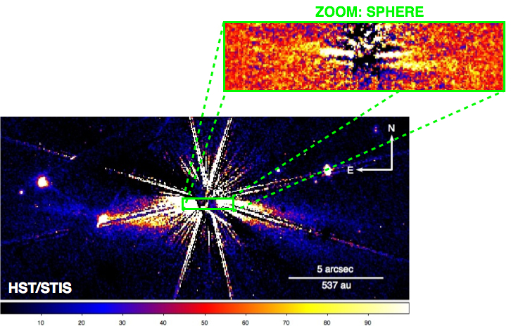
Figure 5: Sketch showing the HST/STIS and the SPHERE images of the debris disk around HIP 67497.

Appendix A Details on the model fitting

We report in Fig. 6 the zones used to compute the $\chi^{2}$ when comparing the disk model to the data. The $\chi^{2}$ for the single belt modelling is computed in the region between the plain green ellipse and the dashed green ellipse. It contains 1041 pixels, or 118 resolution elements. For the case of the model of the outer ring, the $\chi^{2}$ is computed in the region between the plain green ellipse and the black ellipse. It contains 3279 pixels, or 390 resolution elements.

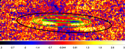
Figure 6: Conservative SNR map showing the regions used to compute the chi square

.

The Fig. 7 show the $\chi^{2}$ minimization for each of the five free parameters of the single ring model (§ 3.2). The Figure 8 show the $\chi^{2}$ minimization for the free parameters of the models with two belts, or one belt and a halo (§ 3.3). The 1$\sigma$ $\chi^{2}$ levels used to estimate the error bars on each parameters are reported in red.

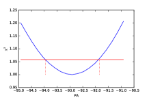
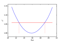
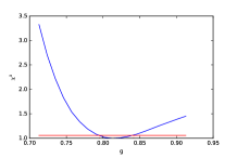
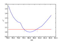
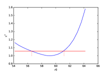
Figure 7: Minimization of the free parameters of the single belt model.

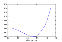
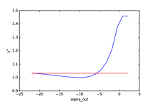
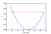
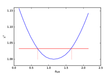
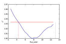
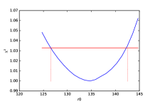
Figure 8: Minimization of the free parameters for the model of a single belt and a halo (left column) and of the model with two belts (right column).

Appendix B Detected point sources and limits

We detect 10 candidate companions (CC) at large separations in the IRDIS H2 and H3 images. Their astrometry and predicted mass – assuming they are bound – are reported in Tab. 4. All those point sources lie outside of the field-of-view of the IFS. None of them is aligned with the disk’s position angle.

The placement of the candidates in color-magnitude diagrams can help to determine if they have both the luminosity and colors typical of cold substellar companions, or if they are rather background objects. Such diagrams have been created for the IRDIS filters (see a description in Mesa et al. 2016). We show the placement of the CCs of HIP 67497 in Figure 10. The CCs #2, 6, and 9 have the luminosities typical of T dwarfs but the colors of MK dwarfs, the most common contaminants. This indicates that these CCs are likely to be background objects. All the remaining CCs, but the CC #1 and 2, are retrieved in the HST/STIS (optical) images of Padgett & Stapelfeldt (2016) and are therefore likely background stars.

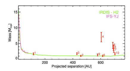
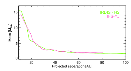
Figure 9: Detection limits (5$\sigma$) for the IFS (spectral PCA) and IRDIS (TLOCI) converted to mass. The candidate companions are reported in red. Top: full separation range. Bottom: zoom at inner working angles.

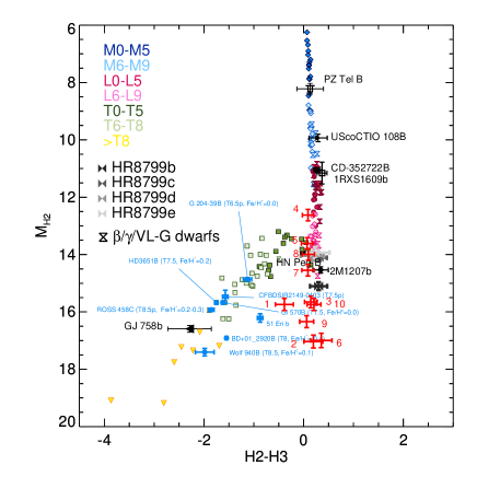
Figure 10: Placement of the candidate companions from Tab. 4 into color-magnitude diagrams.

We estimated the detection limits of the IFS via the injection of fake companions with flat spectra into the datacubes and used the COND evolutionary tracks to convert the derived contrasts to masses (Baraffe et al. 2003). The IRDIS detection limits were estimated from the TLOCI coefficients and the local level of the noise. We report those limits in Fig. 9. The data are sensitive to planetary-mass companions down to 15 au.

Table 4: Photometry and astrometry of point sources. The predicted mass if bound to the star is reported into the last column.

#	Band	Contrast	PA	Sep	$\mathrm{M_{Pred}}$
			(∘)	(mas)	($\mathrm{M_{Jup}}$)
1	H2	13.33$\pm$0.09	185.5$\pm$0.3	1092$\pm$6	2$\pm$1
	H3	13.71$\pm$0.13	185.3$\pm$0.4	1088$\pm$8	2$\pm$1
2	H2	14.62$\pm$0.12	71.9$\pm$0.1	4258$\pm$7	1$\pm$1
	H3	14.42$\pm$0.13	71.9$\pm$0.1	4264$\pm$7	1$\pm$1
3	H2	13.24$\pm$0.08	293.3$\pm$0.1	3996$\pm$3	2$\pm$1
	H3	13.10$\pm$0.07	293.3$\pm$0.1	3998$\pm$3	2$\pm$1
4	H2	10.21$\pm$0.07	100.4$\pm$0.1	5626$\pm$2	7$\pm$2
	H3	10.12$\pm$0.06	100.4$\pm$0.1	5628$\pm$2	7$\pm$2
5	H2	11.20$\pm$0.07	155.8$\pm$0.1	6398$\pm$2	4$\pm$1
	H3	11.13$\pm$0.07	155.8$\pm$0.1	6400$\pm$3	4$\pm$1
6	H2	14.58$\pm$0.16	279.9$\pm$0.1	5721$\pm$6	1$\pm$1
	H3	14.12$\pm$0.12	280.0$\pm$0.1	5724$\pm$7	1$\pm$1
7	H2	12.13$\pm$0.07	285.6$\pm$0.1	6462$\pm$3	3$\pm$1
	H3	12.05$\pm$0.08	285.7$\pm$0.1	6458$\pm$3	3$\pm$1
8	H2	11.58$\pm$0.07	283.7$\pm$0.1	6444$\pm$3	4$\pm$1
	H3	11.48$\pm$0.07	283.7$\pm$0.1	6439$\pm$3	4$\pm$1
9	H2	13.92$\pm$0.09	351.8$\pm$0.1	5376$\pm$4	2$\pm$1
	H3	13.87$\pm$0.09	351.8$\pm$0.1	5375$\pm$5	2$\pm$1
10	H2	13.32$\pm$0.09	342.6$\pm$0.1	6539$\pm$5	2$\pm$1
	H3	13.12$\pm$0.08	342.6$\pm$0.1	6541$\pm$4	2$\pm$1

Appendix C Putative perturbers

We investigate the presence of one, two and three giant planets as responsible for the gap between the two possible belts resolved around HIP 67497 using numerical simulations based on published analytical formulaes. A detailed description will be made in Lazzoni et al. 2016 in prep.

If we make the assumption that one planet on a circular orbit only is responsible for the gap, we find that this planet should have a mass of 20.6 M_Jup and semi-major axis a=90.5 au following Morrison & Malhotra (2015). For the case of an eccentric planet, we used the expressions for the half-width of the chaotic zone $\Delta a$ found by Wisdom (1980) (for planet eccentricity $\leq$0.3) and Mustill & Wyatt (2012) (for eccentricity $>$0.3) as a basis:

$$\Delta a=1.3\times(M_{p}/M_{Star})^{2/7}\times a_{p},$$ (1)

$$\Delta a=1.8\times(M_{p}/M_{Star})^{1/5}\times e^{1/5}\times a_{p},$$ (2)

with $M_{p}$ the planet mass, $M_{star}$ the primary star mass, and $e$ the eccentricity of the disk. In our analysis, we consider the planet to arrive at periastron in the nearest point to the inner belt and at apoastron in the nearest point to the outer one. Then we substitute in the previous expressions for $\Delta a$ the value of the semi-major axis with the positions of periastron and apoastron in turns. In that case, we predict that planets with low eccentricities ($e=0.13$) can have masses below our detection threshold.

We also investigated the case of 2 or 3 equal-mass planets on circular orbits. We considered planets as near as possible to each others (maximum packing, Gladman 1993) in order to have yet a stable system but, at the same time, to obtain completely chaotic regions between the planets such that the disk material could not survive in it. For two planets on circular orbits, we followed the results of Marzari (2014) and found that 2.7 M_Jup equal-mass perturbers with semi-major axis of 73 and 105 au could clear the gap. For the case of a three planet systems with circular orbits, the relations of Marzari (2014) give perturber masses of 0.14 M_Jup and semi-major axis of 64.4, 87.5, and 118.7 au. We considered a last configuration with two equal-mass planets on eccentric orbits, supposing again the maximum packing condition, and following the equations 1 and 2. We find that low masses (0.1-0.4 M_Jup) with quite small eccentricities are needed to dig the entire gap.

We recall that multiple assumptions are made here (equal mass pertubers, maximum packing). Therefore, we believe that a more in depth dynamical analysis of this system is requiered to understand the morphology of the disk (N-body simulations; beyond the scope of this letter).