Cherenkov and parametric (quasi-Cherenkov) radiation from relativistic charged particles moving in crystals formed by metallic wires

Abstract

Until recently, the interaction of electromagnetic waves with crystals built from parallel metallic wires (wire media) was analyzed in the approximation of isotropic scattering of the electromagnetic wave by a single wire. However, if the wires are thick ($kR\sim 1$), electromagnetic wave scattering by a wire is anisotropic, i.e., the scattering amplitude depends on the scattering angle. In this work, we derive the equations that describe diffraction of electromagnetic waves and spontaneous emission of charged particles in wire media, and take into account the angular dependence of scattering amplitude. Numerical solutions of these equations show that the radiation intensity increases as the wire radius is increased and achieves its maximal value in the range $kR\sim 1$. The case when the condition $kR\sim 1$ is fulfilled in the THz frequency range is considered in detail. The calculations show that the instantaneous power of Cherenkov and parametric (quasi-Cherenkov) radiations from electron bunches in the crystal can be tens–hundreds megawatts, i.e., high enough to allow experimental observation as well as possible practical applications.

Introduction

Emission of photons by relativistic charged particles moving in natural or artificial spatially-periodic structures (photonic crystals, metamaterials) has come under intensive theoretical and experimental investigation in recent years [1, 2, 3, 4, 5, 6, 7]. It has been found that spatial-periodic structure of crystals is facilitating for new mechanisms of radiation from a uniformly moving particle to occur in addition to already known Cherenkov and transition radiations: Smith-Purcell effect (diffraction radiation and resonance radiation) [8, 9, 10, 11] and parametric X-ray radiation [1].

Parametric radiation in X-ray frequency range (PXR) caused by particles moving in natural crystals has been theoretically and experimentally studied in numerous works (see [1]) and the references therein. Parametric radiation from a relativistic particle moving in a photonic crystal has been considered in [2, 5]. The theoretical description of PXR is based on Ewald’s and von Laue’s dynamical theory of X-ray diffraction. It is important to note that here the perturbation theory well applies to the description of photon scattering by a single atom, whereas in microwave and optical ranges the perturbation theory does not always apply to describe photon scattering by scatterers that form a photonic crystal (ball, wire, etc.). Nevertheless, as it has been demonstrated in [2], it is possible to derive equations defining process of dynamical diffraction in photonic crystals and to describe the emission of photons from relativistic particles moving in such crystals.

Radiation produced by charged particles moving in crystals built from parallel metallic wires has been studied in [2, 5, 12, 13, 14, 6, 15, 16, 17, 18]. The authors of [6, 15, 16, 17, 18] have considered the case when the wavelength is much greater than the crystal period, and so the diffraction conditions are not fulfilled. Here the crystal was presented as an equivalent uniform medium characterized by certain permittivity and permeability tensors. Inversely, the authors of [2, 5, 12, 13, 14] have not confine themselves to the analysis of long-wave approximation, because diffraction in crystals is paramount for the considered radiation mechanisms (parametric, diffraction). According to the results reported in [5], when the wavelength $\lambda=2\pi/k$ becomes comparable with the wire radius $R$ ($kR\sim 1$) a noticeable increase in the intensity of parametric radiation is observed. As a result, say, electron bunches with $n_{e}\sim 10^{9}$–$10^{11}$ that are produced through laser acceleration can generate GW-level THz pulses in such crystals [5].

Let us note here that until now (see [2, 6, 15, 16, 17], a review article [19] and the reference therein), the authors concerned themselves only with the case when $kR\ll 1$, where scattering of the electromagnetic wave with a “parallel” polarization (vector $\mathbf{E}$ is parallel to the axes of the wires) by a single wire is isotropic, and scattering of a wave with a “perpendicular” polarization can be neglected. The analysis in [5] relies on extrapolation of the results obtained for the theory valid at $kR\ll 1$ to the frequency range $kR\sim 1$, where, generally speaking, scattering by a single wire is anisotropic (the scattering amplitude depends on the scattering angle).

The equations describing the dynamical diffraction theory in 2D crystals that are valid for the case of anisotropic scatering by a single constituent element of the crystal (e.g. wire) were first obtained in [20]. In this paper, we use the theory developed in [20] to give a detailed analysis of refraction and diffraction of waves in crystals built from metallic wires in the case when $kR\sim 1$. We derive the equations that describe spontaneous radiation from charged particles moving in such crystals with due account of angular dependence of the scattering amplitude. Numerical solution of the derived equations shows that, as concluded in [5], the radiation intensity increases with increasing wire radius, achieving its maximum in the range $kR\sim 1$. We give a special consideration to the case when the condition $kR\sim 1$ is fulfilled in THz range of frequencies.

The paper is arranged as follows. The first section describes the general approach that we take to find the characteristics of radiation produced by a charged particle moving in arbitrary targets (photonic crystals). The second section considers the theory of diffraction in photonic crystals built from metallic wires and derives the dispersion equation describing the possible types of waves in the crystal that also holds true in the case when the wires cannot be regarded as thin ($kR\sim 1$). The third section analyzes radiation produced by a charged particle moving in crystals built from metallic wires, at different $kR$.

1 Emission of photons by a charged particle moving in the crystal

Let a relativistic particle of charge $eQ$ move at a constant velocity in a crystal built from parallel metallic wires, as shown in Fig. 1. The crystal thickness $L$ is assumed to be much less than its transverse dimensions and the wire radius $R$ is much less than the crystal periods $a,b$. Let us denote the unit cell area by $\Omega_{2}=ab$.

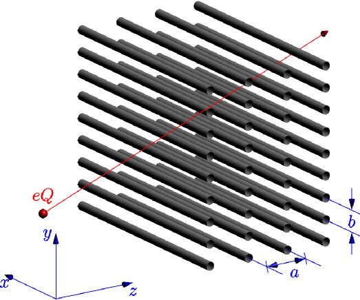
Figure 1: Photonic crystal built from metallic wires and the used coordinate system.

To study the process of emission of electromagnetic waves by a charged particle, we shall use the general approach described in [1, 21, 22]. The spectral density of radiation energy per unit solid angle $W_{\mathbf{n}\omega}$ ($\mathbf{n}=\mathbf{k}/k$), differential number of quanta $\dfrac{d^{2}N}{d\omega d\Omega}\equiv dN_{\mathbf{n}\omega}=W_{\mathbf{n}\omega}/\hbar\omega$, and the polarization characteristics of radiation can be obtained readily if we know the field $\mathbf{E}(\mathbf{r},\omega)$, produced by a charged particle at a large distance $\mathbf{r}$ from the target (crystal):

$$W_{\mathbf{n}\omega}=\frac{cr^{2}}{4\pi^{2}}\left|\mathbf{E}(\mathbf{r},\omega)\right|^{2},$$ (1)

where $c$ is the speed of light.

To find the field $\mathbf{E}(\mathbf{r},\omega)$, we need to solve Maxwell’s equations describing the interaction of particle with a medium. The transverse solution can be found using the Green function $G$ of these equations, which satisfies the relationship (see [1, 21, 22])

$$G=G_{0}+G_{0}\frac{\omega^{2}}{4\pi c^{2}}(\hat{\varepsilon}-1)G.$$ (2)

Here $G_{0}$ is the transverse Green function of Maxwell’s equations at $\hat{\varepsilon}=1$ (it is given, for example, in [23]) and $\hat{\varepsilon}$ is the permittivity tensor of the medium. Using $G$, we can find the field we are concerned with

$$E_{n}(\mathbf{r},\omega)=\int G_{nl}(\mathbf{r},\mathbf{r}^{\prime},\omega)\frac{i\omega}{c^{2}}j_{0l}(\mathbf{r}^{\prime},\omega)d^{3}r^{\prime},$$ (3)

where $n,\,l=x,\,y,\,z$, and $j_{0l}(\mathbf{r},\omega)$ is the Fourier transform of the $l$-th component of the current produced by a moving charged particle.

According to [1, 21], the Green function at $r\rightarrow\infty$ is expressed through the solution of homogeneous Maxwell’s equations containing at infinity a converging spherical wave $E^{(-)s}_{\mathbf{k}l}$:

$$\lim_{r\rightarrow\infty}G_{nl}(\mathbf{r},\mathbf{r}^{\prime},\omega)=\frac{e^{ikr}}{r}\sum\limits_{s}e^{s}_{n}E^{(-)s*}_{\mathbf{k}l}(\mathbf{r}^{\prime},\omega),\\$$ (4)

where $\mathbf{k}=k\frac{\mathbf{r}}{r}$, $\mathbf{e}^{s}$ is the unit polarization vector, $s=1,2$, and $\mathbf{e}^{1}\perp\mathbf{e}^{2}\perp\mathbf{k}$. At $r\rightarrow\infty$, the expression for wave $E^{(-)s}_{\mathbf{k}l}(\mathbf{r}^{\prime})$ takes the form

$$\mathbf{E}_{k}^{(-)s}(\mathbf{r}^{\prime},\omega)=\mathbf{e}^{s}e^{i\mathbf{k}\mathbf{r}^{\prime}}+\mbox{const}\frac{e^{-i{k}{r}^{\prime}}}{r^{\prime}}.$$

The solution $\mathbf{E}_{\mathbf{k}}^{(-)s}(\mathbf{r},\omega)$ is associated with the solution of homogeneous Maxwell’s equations $\mathbf{E}_{\mathbf{k}}^{(+)s}(\mathbf{r},\omega)$ that describes photon scattering by a target and contains at infinity a diverging spherical wave ($\mathbf{E}_{k}^{(+)s}(\mathbf{r},\omega)=\mathbf{e}^{\,\,s}e^{i\mathbf{k}\mathbf{r}}+\mbox{const}\frac{e^{i{k}{r}}}{r}$), [1, 21]:

$$\mathbf{E}^{(-)s*}_{\mathbf{k}}=\mathbf{E}^{(+)s}_{-\mathbf{k}}.$$ (5)

Using (3) and (4), we obtain

$$E_{n}(\mathbf{r},\omega)=\frac{e^{ikr}}{r}\frac{i\omega}{c^{2}}\sum\limits_{s}e^{s}_{n}\int\mathbf{E}^{(-)s*}_{\mathbf{k}}(\mathbf{r}^{\prime},\omega)\mathbf{j}_{0}(\mathbf{r}^{\prime},\omega)d^{3}r^{\prime}=\frac{e^{ikr}}{r}\frac{i\omega}{c^{2}}\sum\limits_{s}e^{s}_{n}\int\mathbf{E}^{(+)s}_{-\mathbf{k}}(\mathbf{r}^{\prime},\omega)\mathbf{j}_{0}(\mathbf{r}^{\prime},\omega)d^{3}r^{\prime}.$$ (6)

Then the spectral density of radiation for photons with polarization vector $\mathbf{e}^{s}$ can be written in the form:

$$W_{\mathbf{n},\omega}^{s}=\frac{\omega^{2}}{4\pi^{2}c^{3}}\left|\int\mathbf{E}^{(-)s*}_{\mathbf{k}}(\mathbf{r},\omega)\mathbf{j}_{0}(\mathbf{r},\omega)d^{3}r\right|^{2},$$ (7)

where

$$\mathbf{j}_{0}(\mathbf{r},\omega)=\int e^{i\omega t}\mathbf{j}_{0}(\mathbf{r},t)dt=eQ\int e^{i\omega t}\mathbf{v}(t)\delta(\mathbf{r}-\mathbf{r}(t))dt,$$ (8)

and $\mathbf{v}(t)$ and $\mathbf{r}(t)$ are the particle velocity and trajectory, respectively.

Substitution of (8) and (5) into (7) finally gives

$$dN^{s}_{\mathbf{n},\omega}=\frac{e^{2}Q^{2}\omega}{4\pi^{2}\hbar c^{3}}\left|\int\mathbf{E}^{(+)s}_{-\mathbf{k}}(\mathbf{r}(t),\omega)\mathbf{v}(t)e^{i\omega t}dt\right|^{2}.$$ (9)

Integration in (9) is performed over the entire domain of particle motion.

Thus, for the analysis of radiation emitted by a particle passing through a photonic crystal, we do not need a complete solution of Maxwell’s equations; suffice it to know the solution of homogeneous Maxwell’s equations describing plane-wave diffraction by the crystal. Solving homogeneous Maxwell’s equations instead of inhomogeneous significantly simplifies the analysis of the radiation problem and enables considering different cases of radiation.

2 Propagation of waves in a crystal built from parallel metallic wires

Let us consider refraction and diffraction of electromagnetic waves in a photonic crystal for the case when $kR\sim 1$. We shall start with solving the problem of plane-wave scattering by a single wire (metallic cylinder), then consider scattering by an one-dimensional grating (a single crystal plane) formed by periodically spaced wires, and finally proceed to deriving the dispersion equation for a infinite crystal.

2.1 Amplitude of electromagnetic wave scattering by a wire

Let a plane electromagnetic wave $\mathbf{E}_{0}=\mathbf{e}_{0}e^{i\mathbf{k}_{1}\mathbf{r}}$ ($\mathbf{e}_{0}$ is the polarization unit vector) be scattered by an infinite cylinder of radius $R$. We shall assume that the cylinder is placed in the medium whose permittivity and permeability are $\varepsilon_{1}$ and $\mu_{1}$, respectively; we shall denote the permittivity and the permeability of the cylinder material by $\varepsilon_{2}$ and $\mu_{2}$, respectively. It is also assumed that the axis of the cylinder is oriented along the $x$-axis of the Cartesian rectangular coordinates and the wave vector of the incident wave is $\mathbf{k}_{1}=(k_{1x},0,k_{1z})$. We shall also introduce a polar coordinate system $(\rho,\varphi)$ in the $(z,y)$-plane using the relations $z=\rho\cos\varphi$ and $y=\rho\sin\varphi$.

It is necessary to consider two possible polarizations of the incident wave :

• transverse electric (TE) polarization, when the vector $\mathbf{E}_{0}$ of the electric field strength is perpendicular to the axis of the cylinder ($E_{0x}=0$). Hereinafter the quantities referring to this polarization will bear the index “$\perp$”;

• transverse magnetic (TM) polarization, when the vector $\mathbf{H}_{0}$ of the magnetic-field strength is perpendicular to the axis of the cylinder ($H_{0x}=0$). Hereinafter the quantities referring to this polarization will bear the index “$\parallel$”, since in this case vector $\mathbf{E}$ has a nonzero component which is parallel to the cylinder axis $x$.

If the incident wave is TM-polarized, then the $x$-component of the field $\mathbf{E}$ can be presented as a series in terms of cylindrical functions [24, 25, 26]:

$$E_{x}=\left\{\begin{aligned} \sum\limits_{n=-\infty}^{\infty}i^{n}J_{n}(k_{\rho}\rho)e^{-in\varphi}+\sum\limits_{n=-\infty}^{\infty}i^{n}a_{n}H_{n}(k_{\rho}\rho)e^{-in\varphi},\;\;\rho\geq R\\ \sum\limits_{n=-\infty}^{\infty}i^{n}b_{n}J_{n}(k^{\prime}_{\rho}\rho)e^{-in\varphi},\;\;\rho\leq R,\end{aligned}\right.$$ (10)

where $J_{n}$ and $H_{n}$ are the Bessel cylindrical function of the $n$-th order and the Hankel cylindrical function of the first kind of the $n$-th order, respectively, $\mathbf{k}_{\rho}=(k_{1y},k_{1z})$, $k_{\rho}=\sqrt{k^{2}\varepsilon_{1}\mu_{1}-k_{1x}^{2}}$, $k^{\prime}_{\rho}=\sqrt{k^{2}\varepsilon_{2}\mu_{2}-k_{1x}^{2}}$, $k=\omega/c$. For brevity, we shall omit the factors $e^{ik_{1x}x}$ in expressions for the field (10), as well as hereinafter in this paper. The component $H_{x}$ of the magnetic field can be represented in a similar way:

$$H_{x}=\left\{\begin{aligned} \sum\limits_{n=-\infty}^{\infty}i^{n}c_{n}H_{n}(k_{\rho}\rho)e^{-in\varphi},\;\;\rho\geq R\\ \sum\limits_{n=-\infty}^{\infty}i^{n}d_{n}J_{n}(k^{\prime}_{\rho}\rho)e^{-in\varphi},\;\;\rho\leq R.\end{aligned}\right.$$ (11)

For ÒÅ-polarization, the expansion (11) must be used for $E_{x}$ and the expansion (10) for $H_{x}$. Other components of the fields are expressed in terms of $E_{x}$ and $H_{x}$ as follows:

$$\left\{\begin{aligned} \mathbf{E}_{\perp}&\equiv&(E_{y},E_{z})&=&\frac{ik_{1x}}{k_{\rho}^{2}}\vec{\nabla}_{\perp}E_{x}-\frac{ik\mu_{1}}{k_{\rho}^{2}}\mathbf{e}_{x}\times\vec{\nabla}_{\perp}H_{x}\\ \mathbf{H}_{\perp}&\equiv&(H_{y},H_{z})&=&\frac{ik_{1x}}{k_{\rho}^{2}}\vec{\nabla}_{\perp}H_{x}+\frac{ik\varepsilon_{1}}{k_{\rho}^{2}}\mathbf{e}_{x}\times\vec{\nabla}_{\perp}E_{x},\end{aligned}\right.$$ (12)

where $\vec{\nabla}_{\perp}=\mathbf{e}_{y}\frac{\partial}{\partial y}+\mathbf{e}_{z}\frac{\partial}{\partial z}$, and $(\mathbf{e}_{x},\mathbf{e}_{y},\mathbf{e}_{z})$ are the unit vectors of the corresponding axes. Equations (12) are valid for $\rho\geq R$; in the case when $\rho<R$, we should replace $k_{\rho}\rightarrow k_{\rho}^{\prime}$, $\varepsilon_{1}\rightarrow\varepsilon_{2}$, $\mu_{1}\rightarrow\mu_{2}$. The unknown coefficients $a_{n}$, $b_{n}$, $c_{n}$, and $d_{n}$ are found from boundary conditions at $\rho=R$.

Let the condition $|k_{1x}|\ll k_{\rho}$ be fulfilled. Then for the coefficients $a_{n}^{\parallel}$ and $a_{n}^{\perp}$ (i.e., the expansion coefficients for the electric field outside the cylinder in the case of TM-polarization ($\parallel$) and for the magnetic field in the case of TE-polarization ($\perp$)), we can obtain the following approximate expressions (see [24, 26]):

$$\left\{\begin{aligned} a_{n}^{\parallel}\approx\frac{-J_{n}(k^{\prime}_{\rho}R)J^{\prime}_{n}(k_{\rho}R)+\sqrt{\frac{\varepsilon}{\mu}}J^{\prime}_{n}(k^{\prime}_{\rho}R)J_{n}(k_{\rho}R)}{J_{n}(k^{\prime}_{\rho}R)H^{\prime}_{n}(k_{\rho}R)-\sqrt{\frac{\varepsilon}{\mu}}J^{\prime}_{n}(k^{\prime}_{\rho}R)H_{n}(k_{\rho}R)},\\ a_{n}^{\perp}\approx\frac{-J_{n}(k^{\prime}_{\rho}R)J^{\prime}_{n}(k_{\rho}R)+\sqrt{\frac{\mu}{\varepsilon}}J^{\prime}_{n}(k^{\prime}_{\rho}R)J_{n}(k_{\rho}R)}{J_{n}(k^{\prime}_{\rho}R)H^{\prime}_{n}(k_{\rho}R)-\sqrt{\frac{\mu}{\varepsilon}}J^{\prime}_{n}(k^{\prime}_{\rho}R)H_{n}(k_{\rho}R)},\end{aligned}\right.$$ (13)

where $\varepsilon=\varepsilon_{2}/\varepsilon_{1}$, $\mu=\mu_{2}/\mu_{1}$. Formulas (13) are exact for $n=0$. If $n\neq 0$, these formulas are exact only when $k_{1x}=0$, whereas at small values of $k_{1x}$ provide the relative error of the order of $\frac{|k_{1x}|}{k_{\rho}}$.

For a wire made from a nonmagnetic metal and placed in a vacuum, the permeability $\mu$ and the permittivity $\varepsilon$ in (13) should be taken as $\mu=1$ and $\varepsilon=1+i\frac{4\pi\sigma}{\omega}$, where $\sigma$ is the conductivity of the metal. Let us write the expressions for the coefficients $a_{n}$ in the case of perfectly conducting wires for their particular simple form. Since the permittivity $\varepsilon\rightarrow i\infty$ as $\sigma\rightarrow\infty$, then from (13) we find

$$\left\{\begin{aligned} a_{n}^{\parallel}=-\frac{J_{n}(k_{\rho}R)}{H_{n}(k_{\rho}R)},\\ a_{n}^{\perp}=-\frac{J^{\prime}_{n}(k_{\rho}R)}{H^{\prime}_{n}(k_{\rho}R)}.\end{aligned}\right.$$ (14)

Let us pay attention to the fact that if the incident plane wave is TM(TE)-polarized, then in the case of perfectly conducting wire, the scattering field is also completely TM(TE)-polarized ($H_{x}=0$ or $E_{x}=0$, respectively). But this is not so in the general case when $\varepsilon$ is an arbitrary value. For example, when a TM-polarized wave is incident onto the wire (i.e., $H_{x,inc}=0$), then in the series expansion of the scattering field $H_{x,sc}=\sum\limits_{n=-\infty}^{\infty}i^{n}c_{n}^{\parallel}H_{n}(k_{\rho}\rho)e^{-in\varphi}$, the coefficients $c_{n}^{\parallel}$, generally speaking, differ from zero (except for $c_{0}^{\parallel}$). Thus, in this example, the TM-polarized wave incident on the wire produces a diffracted one that contains the components with TM- and TE-polarizations with their amplitudes determined by the coefficients $a_{n}^{\parallel}$ and $c_{n}^{\parallel}$, respectively. It can be shown, however, that in the case under consideration, at $|k_{1x}|\ll k_{\rho}$, the amplitudes $|c_{n}|\ll|a_{n}|$, and so can be neglected.

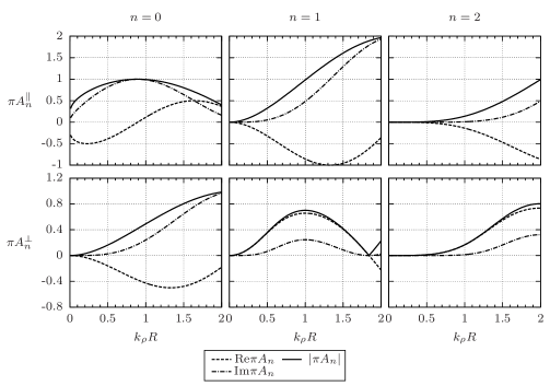
Figure 2: The amplitudes $A_{0}$, $A_{1}$ and $A_{2}$ of electromagnetic wave scattering by a perfectly conducting wire versus $k_{\rho}R$ for two polarizations

Using the asymptotic forms for Hankel functions of large argument and the integral representation of Hankel functions [23, 27], the expressions for $E_{x}$ and $H_{x}$ at large distances from the axis of the cylinder ($k\rho\gg 1$) can be written as

$$\Psi=\left\{\begin{aligned} E_{x}\\ H_{x}\end{aligned}\right\}=e^{i\mathbf{k}_{\rho}\boldsymbol{\rho}}+\left\{\begin{aligned} A^{\parallel}(\varphi)\\ A^{\perp}(\varphi)\end{aligned}\right\}\times\int\limits_{-\infty}^{\infty}\frac{e^{ik\sqrt{\rho^{2}+x^{2}}}}{\sqrt{\rho^{2}+x^{2}}}\mathrm{d}x,$$ (15)

where

$$A^{\parallel(\perp)}(\varphi)=-\frac{i}{\pi}\left(a_{0}^{\parallel(\perp)}+2\sum\limits_{n=1}^{\infty}a_{n}^{\parallel(\perp)}\cos(n\varphi)\right)\equiv\sum\limits_{n=0}^{\infty}A_{n}^{\parallel(\perp)}\cos(n\varphi).$$ (16)

Other unknown components of the fields can be expressed in terms of $E_{x}$ and $H_{x}$ using (12). Following the analogy of a three-dimensional case, by $A(\varphi)$ we shall mean the amplitude of scattering of the electromagnetic wave by a cylinder at an angle $\varphi$ [28].

Figure 2 exemplifies the expansion coefficients $A_{n}$ for the amplitudes of scattering by a perfectly conducting cylinder as a function of $k_{\rho}R$ (they have a similar form for a cylinder made from a finite-conductivity metal). It may be seen that in the range $0<k_{\rho}R\lesssim 1$, we can take account only of the expansion terms $n=0,1$ to consider scattering by a cylinder, because other terms are small. So the expression for a wave scattered by a wire with the coordinates $\mathbf{\rho}_{0}=(y_{0},z_{0})$ can be written in the form:

$$\Psi=e^{i\mathbf{k}_{\rho}\boldsymbol{\rho}}+i\pi A_{0}H_{0}(k_{\rho}|\boldsymbol{\rho}-\boldsymbol{\rho}_{0}|)-\pi A_{1}H_{1}(k_{\rho}|\boldsymbol{\rho}-\boldsymbol{\rho}_{0}|)\cos(\mathbf{k}_{\perp},\boldsymbol{\rho}-\boldsymbol{\rho}_{0}),$$ (17)

where the upper index of the scattering amplitude is omitted for simplicity. In the case when $k_{\rho}R\gtrsim 1$, we need to consider many terms ($n=0,1,2,...$) in expansion of the scattering amplitude (16), and the expression for a wave scattered by the wire becomes quite complicated. In our further analysis we shall confine ourselves to the case when $0<k_{\rho}R\lesssim 1$, and scattering by a single wire can be described by equation (17).

2.2 Scattering of electromagnetic waves by one-dimensional grating

Now, let us consider scattering of a plane wave by one-dimensional grating formed by periodically spaced parallel wires (Fig. 3).

Figure 3: Scattering of a plane wave by a one-dimensional grating formed by metallic wires

Let the coordinates of the wire axes be $\boldsymbol{\rho}_{n}=(z_{n},y_{n})$, $y_{n}=bn$, $z_{n}=0$, where $b$ is the grating period, and the wave vector of incident wave $\mathbf{k}_{1}=(k_{x},k_{y},k_{z})$ (the index “$1$” on the components of the vector is omitted). The general solution for the wave scattered by the grating has the form

$$\Psi=e^{i\mathbf{k}_{\rho}\boldsymbol{\rho}}+i\pi F_{0}\sum\limits_{n=-\infty}^{\infty}e^{ik_{y}bn}H_{0}(k_{\rho}|\boldsymbol{\rho}-\boldsymbol{\rho}_{n}|)-\pi F_{1}\sum\limits_{n=-\infty}^{\infty}e^{ik_{y}bn}H_{1}(k_{\rho}|\boldsymbol{\rho}-\boldsymbol{\rho}_{n}|)\cos\varphi_{n}\\ -\pi F^{\prime}_{1}\sum\limits_{n=-\infty}^{\infty}e^{ik_{y}bn}H_{1}(k_{\rho}|\boldsymbol{\rho}-\boldsymbol{\rho}_{n}|)\sin\varphi_{n},$$ (18)

where summation is made over the coordinates $\boldsymbol{\rho}_{n}$ of all wires, and the amplitudes $F_{0}$, $F_{1}$, and $F^{\prime}_{1}$ are independent of the position of the wire (index $n$) because the grating is assumed to be infinite.

The cylindrical wave of amplitude $F(\varphi_{n})=e^{ik_{y}bn}(F_{0}+F_{1}\cos\varphi_{n}+F^{\prime}_{1}\sin\varphi_{n})$ diverging from the $n$-th wire is produced through scattering by this wire of two waves: 1) the incident plane wave and 2) the sum of cylindrical waves (of amplitudes $F(\varphi_{m})$, $m\neq n$) coming from all other wires. Scattering of the initial plane wave by the wire is described by the expression (17); to describe scattering of cylindrical waves, we can also use (17) provided that each cylindrical wave is presented as a superposition of plane waves [20]. In a similar manner as in [20], formulation a system of linear algebraic equations for $F_{0}$, $F_{1}$, and $F^{\prime}_{1}$, enables us to find

$$\left\{\begin{aligned} F_{0}=F_{0}(k_{y},k_{\rho})&=A_{0}\frac{1+A_{1}(S_{3}+S_{2}k_{y}/k_{\rho}-S_{1})}{1-S_{1}A_{0}-(S_{1}-S_{3})A_{1}-A_{0}A_{1}(S_{1}S_{3}+S_{2}^{2}-S_{1}^{2})},\\ F_{1}=F_{1}(k_{y},k_{\rho})&=A_{1}\frac{k_{z}/k_{\rho}}{1-A_{1}S_{3}},\\ F^{\prime}_{1}=F^{\prime}_{1}(k_{y},k_{\rho})&=A_{1}\frac{k_{y}/k_{\rho}+A_{0}(S_{2}-S_{1}k_{y}/k_{\rho})}{1-S_{1}A_{0}-(S_{1}-S_{3})A_{1}-A_{0}A_{1}(S_{1}S_{3}+S_{2}^{2}-S_{1}^{2})},\end{aligned}\right.$$ (19)

where $S_{1}$, $S_{2}$, and $S_{3}$ are

$$S_{1}=i\pi\sum\limits_{n=1}^{\infty}H_{0}(k_{\rho}bn)(e^{ik_{y}bn}+e^{-ik_{y}bn})=\frac{2i\pi}{k_{z0}b}-i\pi+2\left(\log\frac{k_{\rho}b}{4\pi}+C\right)+\sum\limits_{n\neq 0}\left\{\frac{2i\pi}{k_{zn}b}-\frac{1}{|n|}\right\},$$ (20)

$$S_{2}=\pi\sum\limits_{n=1}^{\infty}H_{1}(k_{\rho}bn)(e^{ik_{y}bn}-e^{-ik_{y}bn})=-2\frac{k_{y}}{k_{\rho}}+\frac{i\pi}{k_{\rho}b}\sum\limits_{n=-\infty}^{\infty}\left\{\frac{k_{y,-n}}{k_{z,-n}}+\frac{k_{yn}}{k_{zn}}\right\},$$ (21)

$$S_{3}=i\pi\sum\limits_{n=1}^{\infty}\frac{H_{1}(k_{\rho}bn)}{k_{\rho}bn}(e^{ik_{y}bn}+e^{-ik_{y}bn})=\frac{2i\pi}{k_{\rho}b}\frac{k_{z0}}{k_{\rho}}-\frac{i\pi}{2}+\left(\log\frac{k_{\rho}b}{4\pi}+C-\frac{1}{2}+\frac{k_{y}^{2}}{k_{\rho}^{2}}+\frac{2\pi^{2}}{3k_{\rho}^{2}b^{2}}\right)+\\ +\frac{2\pi}{k_{\rho}b}\sum\limits_{n\neq 0}\left\{\frac{ik_{zn}}{k_{\rho}}+\frac{|k_{yn}|}{k_{\rho}}-\frac{k_{\rho}b}{4\pi|n|}\right\}.$$ (22)

In these formulas $C\approx 0.5772$ is the Euler constant, $k_{yn}=k_{y}-2\pi n/b$, and $k_{zn}=\sqrt{k_{\rho}^{2}-k_{yn}^{2}}$. The root is taken arithmetically, while in the case when the radicand is negative, we assume that $\sqrt{-|\{...\}|}=+i\sqrt{|\{...\}|}$. Let us note that for $k_{y}b=\pi n$ the expressions (19) simplify appreciably, because in this case $S_{2}=0$.

Let us concentrate on the analysis of scattering of a TM-polarized wave. Using the Poisson summation formula in (18), we can obtain the following expressions for the electric field $\mathbf{E}$ in the case of scattering by a one-dimensional grating of a plane TM-polarized wave of unit amplitude:

$$E_{x} =\frac{k_{\rho}}{k_{1}}\left\{e^{i\mathbf{k}_{\rho}\boldsymbol{\rho}}+\sum\limits_{n=-\infty}^{\infty}\left(F_{0}+F_{1}\frac{k_{zn}}{k_{\rho}}\operatorname{sgn}z+F^{\prime}_{1}\frac{k_{yn}}{k_{\rho}}\right)\frac{2i\pi}{k_{zn}b}e^{ik_{yn}y}e^{ik_{zn}|z|}\right\},$$ (23)

$$E_{y} =-\frac{k_{x}}{k_{1}}\left\{\frac{k_{y}}{k_{\rho}}e^{i\mathbf{k}_{\rho}\boldsymbol{\rho}}+\sum\limits_{n=-\infty}^{\infty}\left(F_{0}+F_{1}\frac{k_{zn}}{k_{\rho}}\operatorname{sgn}z+F^{\prime}_{1}\frac{k_{yn}}{k_{\rho}}\right)\frac{2i\pi}{k_{zn}b}\frac{k_{yn}}{k_{\rho}}e^{ik_{yn}y}e^{ik_{zn}|z|}\right\},$$

$$E_{z} =-\frac{k_{x}}{k_{1}}\left\{\frac{k_{z}}{k_{\rho}}e^{i\mathbf{k}_{\rho}\boldsymbol{\rho}}+\sum\limits_{n=-\infty}^{\infty}\left(F_{0}+F_{1}\frac{k_{zn}}{k_{\rho}}\operatorname{sgn}z+F^{\prime}_{1}\frac{k_{yn}}{k_{\rho}}\right)\frac{2i\pi}{k_{zn}b}\frac{k_{zn}}{k_{\rho}}e^{ik_{yn}y}e^{ik_{zn}|z|}\operatorname{sgn}z\right\}.$$

To help grasp the physical meaning of the expressions (23) more readily, we can write them in a simpler, more compact form

$$\mathbf{E}(\mathbf{r})=\mathbf{e}_{0}e^{i\mathbf{k}_{1}\mathbf{r}}+\sum\limits_{n=-\infty}^{\infty}\mathbf{e}_{n}^{\pm}\Phi_{n}^{\pm}e^{i\mathbf{k}_{n}^{\pm}\mathbf{r}},$$ (24)

where $\mathbf{e}_{0}$ is the polarization unit vector of the wave incident onto the grating, $\mathbf{e}_{n}^{\pm}=\frac{k_{\rho}}{k_{1}}\mathbf{e}_{x}-\frac{k_{x}k_{yn}}{k_{1}k_{\rho}}\mathbf{e}_{y}\mp\frac{k_{x}k_{zn}}{k_{1}k_{\rho}}\mathbf{e}_{z}$ are the polarization unit vectors of waves diverging from the grating (scattered waves), $\mathbf{k}_{n}^{\pm}=(k_{x},k_{yn},\pm k_{zn})$ are their wave vectors, and $\Phi_{n}^{\pm}$ are their amplitudes:

$$\left\{\begin{aligned} \Phi_{n}^{+}&=\frac{2i\pi}{k_{zn}b}\left(F_{0}+F_{1}\frac{k_{zn}}{k_{\rho}}+F^{\prime}_{1}\frac{k_{yn}}{k_{\rho}}\right)=\frac{2i\pi}{k_{zn}b}F(\phi_{n}),\\ \Phi_{n}^{-}&=\frac{2i\pi}{k_{zn}b}\left(F_{0}-F_{1}\frac{k_{zn}}{k_{\rho}}+F^{\prime}_{1}\frac{k_{yn}}{k_{\rho}}\right)=\frac{2i\pi}{k_{zn}b}F(\pi-\phi_{n}),\end{aligned}\right.$$ (25)

where $F(\varphi)=F_{0}+F_{1}\cos\varphi+F^{\prime}_{1}\sin\varphi$ is the effective amplitude of wave scattering by the wire of the grating, $\sin\phi_{n}=\frac{k_{yn}}{k_{\rho}}$, $\cos\phi_{n}=\frac{k_{zn}}{k_{\rho}}$. The sign “$+$” in (24)-(25) refers to the case $z>0$, whereas the sign “$-$” refers to the case $z<0$.

Formula (24) reflects a simple physical fact: in a general case, diffraction of a plane wave having a unit amplitude at a 1D periodic grating gives rise to a set of diverging from the grating plane waves whose amplitudes are $\Phi_{n}^{\pm}$. As follows from the expression for $\mathbf{k}_{n}^{\pm}$, the $y$-components of wave vectors of the scattered waves differ from one another by the reciprocal lattice vector $\tau_{y}=\frac{2\pi n}{b}$. We shall note here that for chaotically placed in the $z$-plane wires (by contrast to periodically placed) there would appear two plane waves; transmitted through and mirror-reflected from the wire array (with wave vectors $\mathbf{k}_{0}^{+}\equiv\mathbf{k}_{1}=(k_{x},k_{y},k_{z})$ and $\mathbf{k}_{0}^{-}=(k_{x},k_{y},-k_{z})$, respectively).

We should also state that at $|k_{yn}|>k_{\rho}$, the wave with index $n$ in (24) is evanescent wave, so at large distances from the grating (at sufficiently large $|z|$), summation in (24) should be confined only to such values of $n$ at which $|k_{yn}|<k_{\rho}$. However, in analyzing the propagation of waves in a 2D crystal, it may be essential that the evanescent waves be taken into account, particularly if the crystal period along the $z$ direction is not large enough, and so here we use the complete expressions for the field (23)-(24).

2.3 Diffraction and refraction in crystals at arbitrary scattering amplitudes

Let now a plane wave with TM polarization be scattered by two gratings instead of one. The gratings are placed at a distance $a$ from one another in a medium whose permittivity and permeability are $\varepsilon_{1}$ and $\mu_{1}$, respectively (Fig. 4). The general solution has a similar form as (23)-(24) i.e., for the $E_{x}$-component of the field $\mathbf{E}$ we can write

$$E_{x}=\frac{k_{\rho}}{k_{1}}e^{i\mathbf{k}_{1}\mathbf{r}}+\frac{k_{\rho}}{k_{1}}\sum\limits_{n}\Phi_{n1}^{\pm}e^{i\mathbf{k}_{n}^{\pm}(\mathbf{r}-\mathbf{z}_{1})}+\frac{k_{\rho}}{k_{1}}\sum\limits_{n}\Phi_{n2}^{\pm}e^{i\mathbf{k}_{n}^{\pm}(\mathbf{r}-\mathbf{z}_{2})},$$ (26)

where $\mathbf{z}_{1}=\mathbf{0}$, $\mathbf{z}_{2}=a\mathbf{e}_{z}$ are the vectors defining the positions of the first and second gratings, respectively; the sign “$+$” or “$-$” in the first sum is chosen according to the sign of the $z$-coordinate, whereas in the second sum the sign is chosen according to the sign of the difference $(z-a)$. The remaining components of the field can be expressed in terms of $E_{x}$ using (12) in a similar manner as was done earlier in this paper.

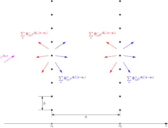
Figure 4: Scattering of a plane wave by two one-dimensional gratings

The unknown amplitudes $\Phi_{n1}^{\pm}$ and $\Phi_{n2}^{\pm}$ can be expressed in terms of the amplitudes $\Phi_{n}^{\pm}$ calculated for the case of scattering by a single grating. We should bear in mind here that each grating scatters not only the initial plane wave $E_{x0}\equiv\Psi_{0}=\frac{k_{\rho}}{k_{1}}e^{i\mathbf{k}_{1}\mathbf{r}}$, but also waves coming from the other grating (see Fig. 4). For example, the first grating scatters the wave $\Psi_{0}+\Psi_{2}$, where

$$\Psi_{2}=\frac{k_{\rho}}{k_{1}}\sum\limits_{n}\Phi_{n2}^{-}e^{i\mathbf{k}_{n}^{-}(\mathbf{r}-\mathbf{z}_{2})}.$$

As a result, we have a set of plane waves diverging from the first grating:

$$\Psi_{1}^{sc}=\frac{k_{\rho}}{k_{1}}\sum\limits_{n}\Phi_{n1}^{\pm}e^{i\mathbf{k}_{n}^{\pm}(\mathbf{r}-\mathbf{z}_{1})}.$$

in a similar way, the second grating is affected by the wave $\Psi_{0}+\Psi_{1}$, where

$$\Psi_{1}=\frac{k_{\rho}}{k_{1}}\sum\limits_{n}\Phi_{n1}^{+}e^{i\mathbf{k}_{n}^{+}(\mathbf{r}-\mathbf{z}_{1})},$$

and as a result, we have a scattered wave

$$\Psi_{2}^{sc}=\frac{k_{\rho}}{k_{1}}\sum\limits_{n}\Phi_{n2}^{\pm}e^{i\mathbf{k}_{n}^{\pm}(\mathbf{r}-\mathbf{z}_{2})}.$$

Knowing the law describing scattering of a unit-amplitude plane wave by a single grating (see (24)-(25)), we can write a system of linear algebraic equations for finding $\Phi_{n1}$ and $\Phi_{n2}$.

Let us consider a very simple example of normal incidence of wave onto a grating when $\mathbf{k}_{1}=(0,0,k_{1})$ and $k_{\rho}=k_{1}$. Let the wave number satisfies the condition $k_{1}b<2\pi$; then in (24) all the waves with $|n|>0$ are evanescent and can be neglected if the distance $a$ between the gratings is large enough. Taking into account that for normal incidence $F^{\prime}_{1}=0$ (see (19)) and $\Phi_{0}^{\pm}=\frac{2i\pi}{k_{1}b}(F_{0}\pm F_{1})$, expressions (24)–(25) yield the following equation for scattering by a single grating placed at $z=z_{0}$

$$E_{x}\approx e^{ik_{1}z}+\frac{2i\pi}{k_{1}b}\left(F_{0}+F_{1}\operatorname{sgn}(z-z_{0})\right)e^{ik_{1}|z-z_{0}|}.$$ (27)

In the case of scattering by two gratings, $\Phi_{0m}^{\pm}=\frac{2i\pi}{k_{1}b}(F_{0m}\pm F_{1m})$, where $m=1,2$ and the earlier written formulas for $\Psi_{0}$, $\Psi_{1}$, $\Psi_{2}$ take the form

$$\Psi_{0}(z)=e^{ik_{1}z},\;\Psi_{1}(z)=\frac{2i\pi}{k_{1}b}\left(F_{01}+F_{11}\right)e^{ik_{1}|z-z_{1}|},\;\Psi_{2}(z)=\frac{2i\pi}{k_{1}b}\left(F_{02}-F_{12}\right)e^{ik_{1}|z-z_{2}|}.$$ (28)

Now we can write the sought system of equations as:

$$\left\{\begin{aligned} F_{01}&=F_{0}\cdot\left[\Psi_{0}(z_{1})+\Psi_{2}(z_{1})\right],\\ F_{11}&=F_{1}\cdot\left[\Psi_{0}(z_{1})-\Psi_{2}(z_{1})\right],\\ F_{02}&=F_{0}\cdot\left[\Psi_{0}(z_{2})+\Psi_{1}(z_{2})\right],\\ F_{12}&=F_{1}\cdot\left[\Psi_{0}(z_{2})+\Psi_{1}(z_{2})\right].\end{aligned}\right.$$ (29)

Here the sign “$-$” before the second term in the second equation is because the wave $\Psi_{2}(z)$ is incident onto the first grating from the positive values of $z$ (it propagate in the direction opposite to that of the wave $\Psi_{0}$).

Taking account of evanescent waves and generalization of the obtained results to the case of arbitrary (non-normal) incidence of the initial wave onto the gratings requires cumbersome arithmetic transformations but do not present serious difficulties. The same refers to the case when there are several ($M$) gratings instead of two. The general solution for the field $E_{x}$ in here has the form

$$E_{x} =\frac{k_{\rho}}{k_{1}}\left\{e^{i\mathbf{k}_{\rho}\boldsymbol{\rho}}+\sum\limits_{n,m}\left(F_{0m}+F_{1m}\frac{k_{zn}}{k_{\rho}}\operatorname{sgn}(z-z_{m})+F^{\prime}_{1m}\frac{k_{yn}}{k_{\rho}}\right)\frac{2i\pi}{k_{zn}b}e^{ik_{yn}y}e^{ik_{zn}|z-z_{m}|}\right\},$$ (30)

where $z_{m}=(m-1)a$, the summation over $m$ is made from 1 to $M$ (i.e., over all gratings), and $F_{0m}$, $F_{1m}$, and $F^{\prime}_{1m}$ are found from the system of linear equations:

$$\frac{F_{0m}}{F_{0}} =e^{ik_{z}z_{m}}+\sum\limits_{n\neq m}\sum\limits_{l}e^{ik_{zl}|z_{m}-z_{n}|}\frac{F_{0}(k_{yl})}{F_{0}(k_{y0})}\frac{2i\pi}{k_{zl}b}\left(F_{0n}+F_{1n}\frac{k_{zl}}{k_{\rho}}\operatorname{sgn}(m-n)+F^{\prime}_{1n}\frac{k_{yl}}{k_{\rho}}\right),$$ (31)

$$\frac{F_{1m}}{F_{1}} =e^{ik_{z}z_{m}}+\sum\limits_{n\neq m}\sum\limits_{l}e^{ik_{zl}|z_{m}-z_{n}|}\frac{F_{1}(k_{yl})}{F_{1}(k_{y0})}\frac{2i\pi}{k_{zl}b}\left(F_{0n}\operatorname{sgn}(m-n)+F_{1n}\frac{k_{zl}}{k_{\rho}}+F^{\prime}_{1n}\frac{k_{yl}}{k_{\rho}}\operatorname{sgn}(m-n)\right),$$

$$\frac{F^{\prime}_{1m}}{F^{\prime}_{1}} =e^{ik_{z}z_{m}}+\sum\limits_{n\neq m}\sum\limits_{l}e^{ik_{zl}|z_{m}-z_{n}|}\frac{F^{\prime}_{1}(k_{yl})}{F^{\prime}_{1}(k_{y0})}\frac{2i\pi}{k_{zl}b}\left(F_{0n}+F_{1n}\frac{k_{zl}}{k_{\rho}}\operatorname{sgn}(m-n)+F^{\prime}_{1n}\frac{k_{yl}}{k_{\rho}}\right).$$

This system of equations has a structure very similar to (29) and considers scattering by each ($m$-th) grating of the initial plane wave $\Psi_{0}$ (the first term on the right-hand side of (31)) as well as the waves coming from all other gratings (the second term). These equations are more awkward than (29) because they consider all evanescent waves and the general case of arbitrary (non-normal) incidence onto the grating.

Now let us proceed from a set of $M$-number of one-dimensional gratings to an infinite (in the $z$ direction) crystal. We shall consider the problem of finding the refractive index of an infinite crystal as an eigenvalue problem as proposed by P.P. Ewald in the development of dynamical theory of diffraction [29, 30, 31]. A coherent wave propagating through a crystal is a result of summation of elementary waves emitted by single wires. Production and propagation of these elementary waves in an infinite, unbounded crystal should be considered as free oscillations (eigenmodes) of the system (crystal) rather than forced ones (excited by an external incident wave) [29, 30, 31]. An important feature of this system is self-consistency manifested in excitation of each wire by the wave field formed by the superposition of elementary waves from all other wires. The same is true not only for single wires, but also for crystal planes (1D gratings discussed earlier in this paper), i.e., each plane starts to emit waves under the effect of the field induced by all other planes. Let us note that similar reasoning was used in the analysis of wave propagation in crystals formed by anisotropically scattering centers in [20, 32] and in [33] â for the case of isotropic scattering.

The above can also be stated as follows. The solution of Maxwell’s equations (30) describes the field induced in crystal through scattering of a plane wave $\mathbf{E}=\mathbf{e}_{0}e^{i\mathbf{k}\mathbf{r}}$, and $F_{0m}$, $F_{1m}$, and $F^{\prime}_{1m}$ in (30) are the solutions of the system of linear nonhomogeneous equations (31), whose column (vector) of constant terms is just determined by the amplitude of the incident wave. To find the eigenmodes of infinite crystal, we need to solve the appropriate system of homogenous equations [34]. According to Bloch’s theorem, we assume that $F_{0n}=F_{00}e^{iq_{z}z_{n}}$, $F_{1n}=F_{10}e^{iq_{z}z_{n}}$, $F^{\prime}_{1n}=F^{\prime}_{10}e^{iq_{z}z_{n}}$, where $q_{z}$ is the unknown $z$-component of the wave vector in the crystal, and $F_{00}$, $F_{10}$, and $F^{\prime}_{10}$ are independent of $z_{n}$. Substitution of these expressions into (31) and elimination of the constant terms $e^{ik_{z}z_{m}}$ corresponding to the wave incident onto the crystal, gives the system of linear equations for $F_{00}$, $F_{10}$, and $F^{\prime}_{10}$, having nonzero solution only when its determinant is zero. After the summation over $n$ (it can be easily done by the formula for geometric series), the substitution of (19) and some other transformations, we obtain the dispersion equation for finding $q_{z}$ in the form

$$\det{D}=0,$$ (32)

where $D$ is a certain $3\times 3$ matrix. Because in the general case the elements of $D$ are quite cumbersome, we shall define them in the Appendix A.

By way of example, let us consider the case of normal incidence of the wave onto the crystal ($k_{x}=k_{y}=0$). The dispersion equation in this case takes the simplest form:

$$\frac{k_{1}b}{2\pi}=-\frac{C_{1}A_{0}}{1+i\pi A_{0}-S^{\prime}_{1}A_{0}}-\frac{C_{5}A_{1}}{1+i\pi A_{1}/2-S^{\prime}_{3}A_{1}}+\frac{2\pi}{k_{1}b}\frac{(C_{3}^{2}-C_{1}C_{5})A_{0}A_{1}}{(1+i\pi A_{0}-S^{\prime}_{1}A_{0})(1+i\pi A_{1}/2-S^{\prime}_{3}A_{1})},$$ (33)

where $S^{\prime}_{1}=\mathrm{Re}\,S_{1}$ and $S^{\prime}_{3}=\mathrm{Re}\,S_{3}$, whereas the functions $C_{1}$, $C_{3}$, and $C_{5}$ depend on the crystal periods $a$ and $b$ and the wave numbers $k_{1}=k\sqrt{\varepsilon_{1}\mu_{1}}$ and $q$ (see Appendix A). Let $q=kn$, where $n$ is the crystal refractive index. If the condition $|n^{2}-\varepsilon_{1}\mu_{1}|\ll 1$ is fulfilled, and $k_{1}a,k_{1}b<2\pi$, then the functions $C_{1}$, $C_{3}$, and $C_{5}$ will be approximately equal to

$$C_{1}\approx C_{5}\approx-C_{3}\approx-\frac{2\sqrt{\varepsilon_{1}\mu_{1}}}{ka(n^{2}-\varepsilon_{1}\mu_{1})}.$$ (34)

Substitution of these values into (33) readily gives the expression for the refractive index $n$ and the crystal’s effective dielectric susceptibility $g_{0}$:

$$g_{0}\equiv n^{2}-1\approx\varepsilon_{1}\mu_{1}-1+\frac{4\pi}{k^{2}ab}\left\{\frac{A_{0}}{1+i\pi A_{0}-S^{\prime}_{1}A_{0}}+\frac{A_{1}}{1+i\pi A_{1}/2-S^{\prime}_{3}A_{1}}\right\},$$ (35)

If $\varepsilon_{1}=\mu_{1}=1$ and the scattering amplitudes are small (so as we can neglect $S^{\prime}_{1}A_{0}$ and $S^{\prime}_{3}A_{1}$), this expression, in fact, coincides with the results obtained in [20].

In a similar way we can solve the dispersion equation in the case when the diffraction conditions in the crystal are fulfilled. Thus derived expressions for effective polarizabilities $g_{\boldsymbol{\tau}}$ (coefficients of Fourier expansion of the crystal’s effective dielectric susceptibility in terms reciprocal lattice vectors $\boldsymbol{\tau}$) are also the same as those given in [20] (see Appendix A).

If the condition $|n^{2}-\varepsilon_{1}\mu_{1}|\ll 1$ for the refractive index is not fulfilled and if the scattering amplitude is not small ($|\pi A_{0,1}|\lesssim 1$), we need to use (52) in Appendix A instead of the approximate expressions (34). Of course in this case, the solutions of the dispersion equations (complete (32) or simplified (33), depending on the geometry of the problem) shall be found numerically.

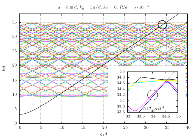
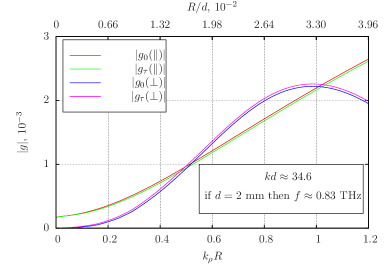
Figure 5: Left: dispersion curves for a crystal built from parallel metallic wires, placed in a vacuum ($\varepsilon_{1}=\mu_{1}=1$); Right: absolute values of effective polarizabilities $g_{0}$ and $g_{\tau}$ versus $k_{\rho}R$ for the selected values of the parameters

Figure 5 gives an example of calculating $g_{0}$ and $g_{\tau}$ using the dispersion equation (32). We consider a crystal with square lattice $a=b\equiv d$ and it is assumed that $k_{y}=\frac{3\pi}{d}$ (i.e., at least the conditions of symmetric two-wave diffraction in Laue geometry are fulfilled in the crystal). The left graph shows the general view of the dispersion curves for a TM-polarized wave at $R/d=5\cdot 10^{-3}$. The black curve represents the solution of the dispersion equation for vacuum ($k^{2}=k_{z}^{2}+k_{y}^{2}$, $k_{z}\equiv q_{z}$). The magnified image shows the range of high frequencies and indicates two roots corresponding to the two close solutions of the dispersion equations. The right graph shows the corresponding absolute values of the effective polarizabilities calculated for the selected geometry with varied parameter $k_{\rho}R$ in the range $0<k_{\rho}R<1.2$. It can be seen that for a TE-polarized wave, $g_{0}^{\perp}$ and $g_{\tau}^{\perp}$ increase as $k_{\rho}R$ is increased, attaining the maximum in the vicinity of $k_{\rho}R\sim 1$. For a TM-polarized wave, the absolute values $|g_{0}^{\parallel}|$ and $|g_{\tau}^{\parallel}|$ increase monotonically. Let us note here that for a TM-polarized wave, the values of $g_{0}$ and $g_{\tau}$ are negative, while for a TE-polarized wave they are positive (i.e., the refractive index for a TE-wave is greater than unity). In the considered case, the maximum values of $g_{0}^{\perp}$ and $g_{\tau}^{\perp}$ even exceed the corresponding values $|g_{0}^{\parallel}|$ and $|g_{\tau}^{\parallel}|$, though in the general case, according to the calculations, the relation between these values can change. However, it is important that in our calculations, the behavior of effective polarizabilities remains almost the same: for a TM-polarized wave $|g_{0}|$ and $|g_{\tau}|$ increase monotonically as $k_{\rho}R$ is increased from $0$ to $1$, while for a TE-polarized wave $|g_{0}|$ and $|g_{\tau}|$ have a maximum at large $k_{\rho}R$ ($k_{\rho}R\sim 1$; the exact position of the maximum may shift within a narrow range.)

3 Radiation in crystals built from wires at $k_{\rho}R\lesssim 1$

3.1 Formulas for spectral-angular distribution

The expressions (30) for the fields and the system (31) derived in the previous sections enable the analysis of photon emission from a charged particle in a crystal built from metallic wires in the case when $k_{\rho}R\sim 1$. Let a particle velocity $\mathbf{v}=(v_{x},v_{y},v_{z})$; then the particle trajectory $\mathbf{r}(t)=\mathbf{v}t$. Let us assume for simplicity that $\varepsilon_{1}=\mu_{1}=1$. Substitution of (30) into the formula for spectral-angular distribution of radiation (9) followed by certain transformation gives

$$\frac{d^{2}N^{s}}{d\Omega d\omega}=\frac{e^{2}Q^{2}}{\hbar c}\cdot\frac{1}{\omega}\cdot|I^{s}|^{2},$$ (36)

where for TM-polarization

$$I^{\parallel}=\frac{1}{k_{\rho}b}\sum\limits_{n}\frac{1}{k_{zn}}\left\{\left(\mathcal{F}_{0n}+\mathcal{F}_{1n}\frac{k_{zn}}{k_{\rho}}+\mathcal{F}^{\prime}_{1n}\frac{k_{yn}}{k_{\rho}}\right)\frac{\mathbf{e}_{x}[\mathbf{k}_{n},[\mathbf{k}_{n},\mathbf{v}]]}{\omega-\mathbf{k}_{n}\mathbf{v}}\right.-\\ -\left.\left(\mathcal{F}_{0n}-\mathcal{F}_{1n}\frac{k_{zn}}{k_{\rho}}+\mathcal{F}^{\prime}_{1n}\frac{k_{yn}}{k_{\rho}}\right)\frac{\mathbf{e}_{x}[\mathbf{k}_{n}^{(-)},[\mathbf{k}_{n}^{(-)},\mathbf{v}]]}{\omega-\mathbf{k}_{n}^{(-)}\mathbf{v}}\right\},$$ (37)

for TE-polarization

$$I^{\perp}=\frac{1}{k_{\rho}b}\sum\limits_{n}\frac{1}{k_{zn}}\left\{\left(\mathcal{F}_{0n}^{\perp}+\mathcal{F}_{1n}^{\perp}\frac{k_{zn}}{k_{\rho}}+\mathcal{F}^{{}^{\prime}\perp}_{1n}\frac{k_{yn}}{k_{\rho}}\right)\frac{\mathbf{e}_{x}[\mathbf{k}_{n},\mathbf{v}]}{\omega-\mathbf{k}_{n}\mathbf{v}}\right.-\\ -\left.\left(\mathcal{F}_{0n}^{\perp}-\mathcal{F}_{1n}^{\perp}\frac{k_{zn}}{k_{\rho}}+\mathcal{F}^{{}^{\prime}\perp}_{1n}\frac{k_{yn}}{k_{\rho}}\right)\frac{\mathbf{e}_{x}[\mathbf{k}_{n}^{(-)},\mathbf{v}]}{\omega-\mathbf{k}_{n}^{(-)}\mathbf{v}}\right\},$$ (38)

$\mathcal{F}_{0n}$, $\mathcal{F}_{1n}$, and $\mathcal{F}^{\prime}_{1n}$ equal

$$\mathcal{F}_{0n}=\sum\limits_{m=1}^{M}F_{0m}e^{i\frac{z_{m}}{v_{z}}(\omega-k_{x}v_{x}-k_{yn}v_{y})},\;\;\mathcal{F}_{1n}=\sum\limits_{m=1}^{M}F_{1m}e^{i\frac{z_{m}}{v_{z}}(\omega-k_{x}v_{x}-k_{yn}v_{y})},\;\;\mathcal{F}^{\prime}_{1n}=\sum\limits_{m=1}^{M}F^{\prime}_{1m}e^{i\frac{z_{m}}{v_{z}}(\omega-k_{x}v_{x}-k_{yn}v_{y})},$$ (39)

where the notations $\mathbf{k}_{n}=(k_{x},k_{yn},k_{zn})$ and $\mathbf{k}_{n}^{(-)}=(k_{x},k_{yn},-k_{zn})$ are introduced.

Formulas (36)-(39) together with the set of equations (31) describe the emission from a charged particle passing through the crystal built from wires. Let us suppose that we have a photonic crystal consisting of a small number of one-dimensional gratings (several tens or hundreds). In this case, the set of equations (31) can be efficiently solved numerically. If (31) is successfully solved and the values of the amplitudes $F_{0m}$, $F_{1m}$, and $F^{\prime}_{1m}$ are found, then the spectral-angular distribution of radiation can be calculated using (36)-(39). But since these expressions in the general form can hardly be integrated analytically, we need to apply the numerical integration when using them for calculating the total intensity of radiation.

To simplify the analysis of the radiation process let us make use of the parameters $g_{0}$, $g_{\boldsymbol{\tau}}$ pre-calculated by the dispersion equation. Let the diffraction conditions in the crystal be violated. If $|g_{0}|\ll 1$, then the wave vector in the crystal $\mathbf{q}\approx\mathbf{k}+\frac{\omega g_{0}}{2c\gamma_{0}}\mathbf{N}$, where $\mathbf{N}$ is the normal to the crystal surface and $\gamma_{0}=\mathbf{k}\mathbf{N}/k$. By solving the boundary-value problem for plane-wave refraction by a crystal plate of thickness $L$ placed at $0<z<L$ we can show that

$$\mathbf{E}_{\mathbf{k}}^{(-)s}\approx\mathbf{e}_{s}e^{i\mathbf{k}\mathbf{r}}\theta(z-L)+\mathbf{e}_{s}e^{i\mathbf{q}\mathbf{r}}e^{i\frac{\omega g_{0}L}{2c\gamma_{0}}}\theta(L-z)\theta(z)+\mathbf{e}_{s}e^{i\mathbf{k}\mathbf{r}}e^{i\frac{\omega g_{0}L}{2c\gamma_{0}}}\theta(-z),$$ (40)

where $\theta(z)$ is the Heaviside function ($\theta(z)=1$ at $z\geq 0$ and $\theta(z)=0$ at $z<0$). Substitution of (40) into (9) yields a well-known expression for spectral-angular distribution of Cherenkov and transition radiations:

$$\frac{d^{2}N^{s}}{d\omega d\Omega}=\frac{e^{2}Q^{2}\omega}{4\pi^{2}\hbar c^{3}}(\mathbf{e}_{s}\mathbf{v})^{2}\left|e^{i\frac{\omega Lg_{0}^{s}}{2c\gamma_{0}}}\left[\frac{1}{\omega-\mathbf{k}\mathbf{v}}-\frac{1}{\omega-\mathbf{q}\mathbf{v}}\right]\left(e^{i(\omega-\mathbf{q}\mathbf{v})\frac{L}{c\gamma_{0}}}-1\right)\right|^{2}.$$ (41)

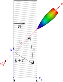
a)

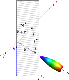
b)

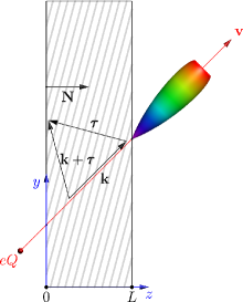
c)

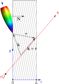
d)

Figure 6: Parametric (quasi-Cherenkov) radiation in photonic crystal for the case of two-wave diffraction in Laue (a, b) and Bragg (c, d) geometries. The $x$-axis is perpendicular to the figure’s plane.

Now, let the two-wave diffraction conditions in the crystal be fulfilled. Substitution of the formulas for $\mathbf{E}_{\mathbf{k}}^{(-)s}$, which are valid in the case of diffraction, into (9) yields the expression for spectral-angular distribution of parametric (quasi-Cherenkov) radiation (see Fig.  6). Because the procedure is fully described in [22, 5], we shall not be concerned discuss it here but shall be concerned with some results only.

According to [5], in the Laue case (when the incident and diffracted waves leave the crystal through the same surface) we have the following equation for parametric radiation at a small angle to particle velocity (Fig. 6(a)):

$$\frac{d^{2}N^{s}_{0}}{d\omega d\Omega} = \frac{e^{2}Q^{2}\omega}{4\pi^{2}\hbar c^{3}}(\mathbf{e}_{s}\mathbf{v})^{2}\left|\sum_{\mu=1,2}\xi^{0}_{\mu s}e^{i\frac{\omega}{c\gamma_{0}}\varepsilon_{\mu s}L}\left[\frac{1}{\omega-\mathbf{k}\mathbf{v}}-\frac{1}{\omega-\mathbf{q}_{\mu s}\mathbf{v}}\right]\left(e^{i(\omega-\mathbf{q}_{\mu s}\mathbf{v})\frac{L}{c\gamma_{0}}}-1\right)\right|^{2},$$ (42)

and for radiation in the diffraction direction (Fig. 6(b))

$$\frac{d^{2}N^{s}_{\tau}}{d\omega d\Omega} = \frac{e^{2}Q^{2}\omega}{4\pi^{2}\hbar c^{3}}(\mathbf{e}^{\tau}_{s}\mathbf{v})^{2}\left|\sum_{\mu=1,2}\beta_{1}\xi^{\tau}_{\mu s}e^{i\frac{\omega}{c\gamma_{0}}\varepsilon_{\mu s}L}\left[\frac{1}{\omega-\mathbf{k}_{\tau}\mathbf{v}}-\frac{1}{\omega-\mathbf{q}_{\tau\mu s}\mathbf{v}}\right]\left(e^{i(\omega-\mathbf{q}_{\tau\mu s}\mathbf{v})\frac{L}{c\gamma_{0}}}-1\right)\right|^{2},$$ (43)

where $\mathbf{q}_{\mu s}$ are the roots of the dispersion equation, $\mathbf{k}_{\tau}=((\mathbf{k}+\boldsymbol{\tau})_{\perp},\sqrt{k^{2}-(\mathbf{k}+\boldsymbol{\tau})_{\perp}^{2}})$, $\mathbf{q}_{\tau\mu s}=\mathbf{q}_{\mu s}+\boldsymbol{\tau}$, $\varepsilon_{\mu s}=\gamma_{0}^{2}(q_{z\mu s}/k_{z}-1)$, $\gamma_{0}=\mathbf{k}\mathbf{N}/k$, $\gamma_{1}=(\mathbf{k}+\boldsymbol{\tau})\mathbf{N}/|\mathbf{k}+\boldsymbol{\tau}|$, $\beta_{1}=\gamma_{0}/\gamma_{1}$, $\mathbf{N}$ is the normal to the entrance surface of the crystal directed to the crystal’s interior, the subscript “$\perp$” denotes the vector components perpendicular to $\mathbf{N}$, $\mathbf{e}_{1}||[\mathbf{k}\times\boldsymbol{\tau}]$, $\mathbf{e}_{2}||[\mathbf{k}\times\mathbf{e}_{1}]$, and

$$\xi^{0}_{1(2)s}=\mp\frac{2\varepsilon_{2(1)s}-g_{0}^{s}}{2(\varepsilon_{2s}-\varepsilon_{1s})},\;\;\;\xi^{\tau}_{1(2)s}=\pm\frac{g_{\tau}^{s}}{2(\varepsilon_{2s}-\varepsilon_{1s})}.$$

Similar expressions are obtained in [5] for parametric radiation in the Bragg diffraction case, too (when the incident and diffracted waves leave the crystal through the opposite surfaces, Fig. 6(c–d)).

3.2 Cherenkov and transition radiations

Now let us give a more detailed consideration to different radiation cases that occur as charged particles moves uniformly through a crystal built from metallic wires. Let us state, first, that because the crystal’s refractive index for a $TE$-polarized wave is greater than unity, Cherenkov radiation is emitted in the crystal [3, 4]. Moreover, transition radiation is also emitted when a charged particle crosses the “crystal-vacuum” boundary. In our analysis we shall use (41) for spectral-angular distribution of transition and Cherenkov radiations.

For simplicity, we shall assume that the crystal has a square lattice ($a=b\equiv d$). Figure 7 shows the typical values of $g_{0}^{\perp}$ è $g_{0}^{\parallel}$ as a function of the parameter $k_{\rho}R$ calculated by (33) for a crystal made from metallic wires.

Figure 7: Effective polarizability $g_{0}$ as a function of the parameter $k_{\rho}R$ for crystal made from metallic wires with a square lattice (normal incidence; $kd\approx 35.5$, which at $d=2$ mm corresponds to the frequency $0.85$ THz)

As is seen, for a $TE$-polarized wave, $g_{0}>0$, i.e., the crystal’s refractive index for this wave is $n_{\perp}\approx 1+\frac{1}{2}g_{0}^{\perp}>1$. If the particle velocity is less than than the phase velocity $v_{\perp}=c/n_{\perp}$ of a $TE$-wave in crystal, then only transition radiation is emitted as the particle passes through the crystal. But if the particle velocity is greater than the phase velocity of a $TE$-wave, then $\omega-\mathbf{q}\mathbf{v}$ can vanish, and the term in (41) whose denominator contains $\omega-\mathbf{q}\mathbf{v}$ will increase as the crystal thickness is increased. At significantly large $L$ ($L\gg l_{0}=\lambda\gamma^{2}$; $l_{0}$ ($l_{0}$ is the coherent radiation length in the vacuum and $\lambda$ is the wavelength), this term will make the major contribution to the total radiation intensity. This picture fully corresponds to the ordinary Cherenkov radiation emitted as the charged particle moves through optically transparent medium at a velocity greater than the phase velocity of light for this media. As is known, this radiation is emitted at an angle $\theta$ to the direction of the particle velocity determined from the condition $\cos\theta=\frac{1}{\beta n_{\perp}}$, where $\beta=v/c$. In the ultra-relativistic case, when $\gamma\gg 1$, in view of smallness of $g_{0}^{\perp}$ the Cherenkov cone angle for the considered crystal can be written as $\theta_{c}\approx\sqrt{g_{0}^{\perp}}$.

It should be noted, however, that at typical values $\gamma\sim 10^{2}\div 10^{3}$ and $\lambda\sim 0.3$ mm, the coherent length $l_{0}$ takes on rather large values in the range from several meters to several hundreds of meters, so in the general case, to find spectral-angular distribution, we need to consider all terms appearing in (41). By way of example, Figure 8 compares the spectral-angular distributions of Cherenkov and transition radiations calculated considering all terms between the square brackets in (41) with those calculated considering only the first or only the second term. In our calculations the particle Lorentz factor was $\gamma=100$, only radiation of $TE$-polarized wave was considered, and the assumed value of $g_{0}^{\perp}\approx 1.7\cdot 10^{-3}$ corresponded to $k_{\rho}R\approx 0.9$ (see Fig. 7). As is seen, with the selected values of these parameters, the results obtained using the complete formula (41) and those obtained taking into account only the term proportional to $(\omega-\mathbf{q}\mathbf{v})^{-1}$ are almost the same when the crystal thickness $L\gtrsim 1$ m.

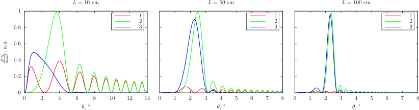
Figure 8: Spectral-angular distributions of Cherenkov and transition radiations in a crystal made from metallic wires for a $TE$-polarized wave: 1 – only the first term between the square brackets in (41) is taken into account, 2 – only the second term between the square brackets in (41) is taken into account, 3 – all terms are taken into account. The given dependence is on the polar angle $\theta$ alone (the polarization factor $\sin^{2}\varphi$ is omitted). Particle Lorentz factor $\gamma=100$, crystal period $d=2$ mm, radiation frequency $f=0.85$ THz, $l_{0}=\lambda\gamma^{2}\approx 3.5$ m, $g_{0}^{\perp}\approx 1.7\cdot 10^{-3}$.

For a $TM$-polarized wave, $g_{0}<0$ (see Fig. 7), and the denominator of the second term in (41) cannot vanish. In this case only transition radiation is possible in the crystal; its spectral-angular distribution is analyzed with due account of all terms in (41).

The total radiation intensity (without separation of contributions coming from Cherenkov and transition radiations) can be found by numerical integration of (41) with respect to angular coordinates and frequency. By way of example we calculated the intensities of Cherenkov and transition radiations in a crystal built from metallic wires using the known values of $g_{0}$ (Fig. 7). To avoid ambiguity, the crystal thickness was set equal to 10 cm, the particle (electron) velocity was perpendicular to the crystal surface, $\gamma=100$. The results are given in Fig. 9.

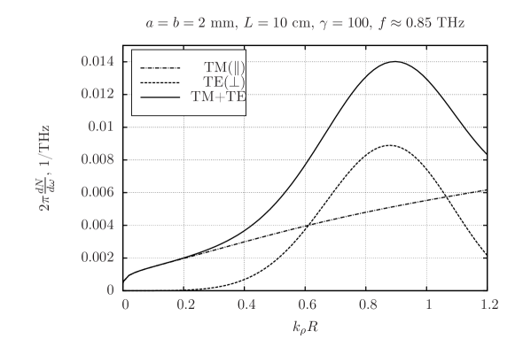
Figure 9: Intensities of transition and Cherenkov radiations in the crystal formed by metallic wires as a function of $k_{\rho}R$. Radiation intensity from $TM$ and $TE$-polarized waves and total radiation intensity (for both polarizations) are shown. The results are obtained by formula (41) with due account of all terms.

As is seen in the plot, the intensity of transition and Cherenkov radiations in a crystal made from metallic wires has a maximum in the vicinity of $k_{\rho}R\sim 1$ that corresponds to the maximum value of $g_{0}^{\perp}$. At $k_{\rho}R\approx 0.9$, in particular, the total radiation intensity for two polarizations is as high as $1.4\cdot 10^{-2}$ photons/THz at the frequency $f=0.85$ THz. Then, for example, in a narrow frequency range from $f_{1}=0.99f$ to $f_{2}=1.01f$ ($\Delta f=0.02f=17$ GHz) the number of photons emitted per one electron is on average $N_{tot}\sim 2.4\cdot 10^{-4}$ photons. Of course, in a wider frequency range, the total number of photons emitted per electron will be greater, achieving , e.g., $N_{tot}\sim 2.4\cdot 10^{-3}$ at $\Delta f=0.2f=170$ GHz. Note here that the intensity of radiation, being proportional to $Q^{2}$ according to (41), is much higher for particles with greater charge ($Q>1$). Thus, for a relativistic nucleus of charge $Q\sim 50$ passing through the same crystal of thickness 10 cm, the intensity of radiation at $k_{\rho}R\sim 1$ increases by more than three orders of magnitude up to more than 1 photon per nucleus [5].

3.3 Parametric (quasi-Cherenkov) radiation

We shall proceed to the discussion of parametric radiation in a crystal made from metallic wires. For definiteness, we shall consider radiation in the case of two-wave symmetric Laue diffraction (see Fig. 6a-b). Here the reciprocal lattice vector is $\boldsymbol{\tau}=\frac{2\pi m}{d}\mathbf{e}_{y}$, where $m$ is the integer, and the Bragg angle $\theta_{B}$ is related to $k_{B}$ as

$$\sin\theta_{B}=\frac{\tau}{2k_{B}}=\frac{\pi m}{kd}.$$ (44)

By way of example we assume that $m=3$ and make use of the above values of the effective polarizabilities $g_{\boldsymbol{\tau}}$ (Fig. 5 right). We also assume that the particle has a charge $Q=1$ (electron, proton, etc.). The intensity of radiation is calculated using (43).

The results of numerical integration of these expressions with respect to frequency and angular coordinates are given in Fig. 10. As is seen, the radiation intensity for $TM$-polarization increases monotonously with $k_{\rho}R$, attaining at $k_{\rho}R=1.2$ the value $N_{\parallel}\approx 2.5\cdot 10^{-4}$ photons/electron (the radiation frequency for the selected crystal period of 2 mm is $0.83$ THz). At large $k_{\rho}R$, the intensity of radiation for a $TE$-polarized wave also increases appreciably, in the considered case exceeding that for $TM$-polarization already at $k_{\rho}R\gtrsim 0.4$ and achieving the maximum value $N_{\perp}\approx 5\cdot 10^{-4}$ photons/electron at $k_{\rho}R\approx 1$. The total (for two polarizations) intensity of radiation also attains its maximum $N_{tot}\approx 7\cdot 10^{-4}$ photons/electron at $k_{\rho}R\approx 1$ (see Fig. 10), which for the selected parameters of the crystal corresponds to the wire radius $R\approx 65\leavevmode\nobreak\$ $\mu$m.

Let us pay attention to the fact that at large $k_{\rho}R$, the contributions to the total intensity coming from $TE$- and $TM$-polarized waves can be comparable (in our case at $k_{\rho}R\sim 1$ the contribution from the $TE$ wave is dominating), whereas for thin wires ($k_{\rho}R\ll 1$), the main contribution to the radiation intensity comes from the $TM$-polarized wave. This is also seen in Fig. 11 showing the angular distribution of parametric radiation. As the parameter $k_{\rho}R$ increases, the angular distribution changes appreciably from the form shown in Fig. 11 (left) at $k_{\rho}R\ll 1$ to a more symmetric form (Fig. 11, center) as the intensities of $TE$- and $TM$-polarized waves become comparable, and finally to a form shown in Fig. 11 (left) as the main generation begins at the $TE$-wave. Let us note that at large Bragg angles, the $TE$-polarized wave can make a significant contribution to the radiation intensity even when $k_{\rho}R\ll 1$, because $A_{0}^{\perp}$ is nonzero (this is what makes the considered case different from parametric X-ray radiation where at $2\theta_{b}=90^{\circ}$ the $\pi$-polarized is absent at all [1])

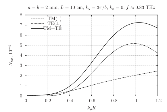
Figure 10: Intensity of parametric radiation (number of photons emitted by one electron passing through the crystal) as a function of radius of the wires composing the crystal.

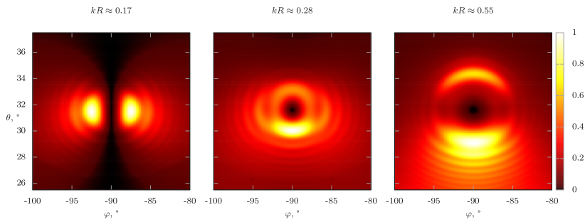
Figure 11: Angular distribution (total for two polarizations) of parametric radiation in the diffraction direction at different $k_{\rho}R$; the crystal thickness is $L=50$ cm, Lorentz factor $\gamma=100$ (electron energy $E=50.5$ MeV).

As the photon absorption length $L_{abs}$ in the considered crystal is large (e.g., in the case of copper wires, the calculation by the dispersion equation gives $\mathop{\mathrm{Im}}\nolimits g_{0}\sim 8.5\cdot 10^{-7}$, which corresponds to $L_{abs}\sim 10^{2}$ m at the frequency $0.83$ THz), the total radiation intensity in the crystal can be increased by increasing the crystal thickness. As an example, Fig. 12 plots the intensity of parametric radiation against the crystal thickness at varied $k_{\rho}R$ for the selected geometry. It is seen that as $L$ increases the radiation intensity also increases, being as high as $6\cdot 10^{-3}$ photons/electron and greater at $k_{\rho}R\sim 1$ and $L=1$ m. In this case, at the selected parameters of the crystal the intensity of radiation from the $TE$-polarized wave is almost twice as large as that from the $TM$-polarized wave. Let us emphasize that at small $k_{\rho}R$, almost the entire radiation is generated at the $TM$-wave, which is obvious from Fig. 12.

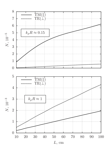
Figure 12: Intensity of parametric radiation as a function of crystal thickness.

Let us take notice of the fact that in our discussion we did not consider the influence of multiple scattering of particles in crystals on radiation process. This influence can be eliminated if a particle moves through a hole made in the crystal or parallel to the crystal surface. In this case, the radiation processes are similar to those occurring in solid crystals, provided that the distance $d$ between the particle and the crystal surface satisfies the condition $d<\frac{\lambda}{4\pi}\beta\gamma$ [21, 9]. In our example, we obtain for $d$ a reasonable value $d\approx 3$ mm at $f=0.83$ THz and $\gamma=100$.

3.4 Radiation from electron bunches

Beams of high-energy particles generated by accelerators usually consist of short particle bunches following one another at certain intervals. Modern acceleration facilities are capable of generating relativistic electron beams with typical bunch duration $t_{b}$ less than $10^{-13}$ s (and as low as $10^{-15}$ s) with the number of electrons in the bunch $N_{e}\sim 10^{9}$ and greater [35, 36, 37]. Such compact bunches (whose size is much less than the wavelength) can emit coherently (as a single particles of charge $Q=N_{e}$), and hence we can expect that proceeding from single electrons to electron bunches will significantly — by a factor of $N_{e}^{2}$ — increase the intensity of parametric radiation [5].

According to [38, 39], the spectral-angular distribution of photons emitted by a bunch of particles moving in a crystal, $\frac{d^{2}N}{d\omega d\Omega}$, is related to that emitted by a single particle, $\frac{d^{2}N_{1}}{d\omega d\Omega}$ as

$$\frac{d^{2}N}{d\omega d\Omega}=N_{e}\frac{d^{2}N_{1}}{d\omega d\Omega}+\frac{d^{2}N_{1}}{d\omega d\Omega}\left|\int e^{-i\mathbf{K}\mathbf{r}}\rho(\mathbf{r})d^{3}\mathbf{r}\right|^{2},$$ (45)

where $\rho(\mathbf{r})$is the bunch density and $N_{e}=\int\rho(\mathbf{r})d^{3}\mathbf{r}$ (integration is performed in the entire bunch volume); the velocity spread in the bunch is neglected. If the direction of the $z$-axis of the rectangular coordinate system coincides with the direction of bunch velocity $\mathbf{v}$, then vector $\mathbf{K}$ in (45) for the forward parametric radiation $\mathbf{K}=(\mathbf{k}_{\perp},\omega/v)$, whereas for radiation in the direction of diffraction $\mathbf{K}=((\mathbf{k}+\boldsymbol{\tau})_{\perp},\omega/v)$, where the subscript “$\perp$” is for vector components perpendicular to the $z$-axis.

In many cases the density of particles in a bunch can be described with good accuracy by normal distribution

$$\rho(\mathbf{r})=\frac{N_{e}}{(\sqrt{2\pi})^{3}\sigma_{\perp}^{2}\sigma_{z}}\exp\left(-\frac{\mathbf{r}_{\perp}^{2}}{2\sigma_{\perp}^{2}}\right)\exp\left(-\frac{z^{2}}{2\sigma_{z}^{2}}\right),$$ (46)

where the root-mean-square deviations $\sigma_{\perp}$ and $\sigma_{z}$ determine the bunch dimensions in transverse and longitudinal directions (relative to the velocity direction), respectively. Such bunches are used, e.g., for producing radiation in free electron lasers [40]. Substitution of the expression for $\rho(\mathbf{r})$ into (45) gives

$$\frac{d^{2}N}{d\omega d\Omega}=N_{e}\frac{d^{2}N_{1}}{d\omega d\Omega}+N_{e}^{2}\frac{d^{2}N_{1}}{d\omega d\Omega}\exp\left(-K_{\perp}^{2}\sigma_{\perp}^{2}-\frac{\omega^{2}}{v^{2}}\sigma_{z}^{2}\right).$$ (47)

By way of example, let us estimate the radiated power of parametric radiation from a relativistic electron bunch passing through a considered crystal made from metallic wires. We shall use the typical bunch parameters available with modern acceleration facilities. For example, according to [40] SwissFEL, X-ray free-electron laser currently being built at the Paul Scherrer Institute can generate electron beams composed of bunches with $N_{e}\approx 1.25\cdot 10^{9}$ (the bunch charge $Q\approx 200$ pC), $\sigma_{z}\approx 9$ $\mu$m (corresponds to the bunch duration of 30 fs), $\sigma_{\perp}\approx 80$ $\mu$m. The plots given in Fig. 11 show that the width of angular distributions of parametric radiation in the selected geometry is within $10^{\circ}$. From this we can readily estimate the maximum value $K_{\perp max}\approx\frac{\omega}{c}\sin 10^{\circ}$ and the minimum value of the exponential factor in the second term in (47): $\exp(-K_{\perp}^{2}\sigma_{\perp}^{2}-\frac{\omega^{2}}{v^{2}}\sigma_{z}^{2})\approx 0.92$ (we considered here that the radiation frequency in the example given in section 3.3 is $f=\omega/2\pi\approx 0.83$ THz). Thus, the main contribution to the total intensity comes from the second term in (47), i.e., the electrons in the bunch emit coherently. Then the instantaneous (peak) power of parametric radiation is $P\approx 0.92\frac{N_{tot}N_{e}^{2}\hbar\omega}{t_{b}}$, where $t_{b}=\sigma_{z}/c\approx 30$ fs is the bunch duration. Substitution of the found maximum value for the crystal of thickness 10 cm $N_{tot}\approx 7\cdot 10^{-4}$, gives $P\approx 18$ MW. Using Fig. 12 we can readily find that as the crystal thickness increases to 1 m, the radiation power increases by almost a factor of 10, achieving the value as high as $P\approx 160$ MW.

For comparison, let us estimate the power of transition and Cherenkov radiations. For parametric radiation, the width of the spectral peak $\Delta\omega/\omega\sim\sqrt{\gamma^{-2}+|g_{0}|}\approx 0.04$ [41]. Using the results of section 3.2, we obtain that the electron passing through the crystal of thickness 10 cm emits in the same frequency range on average $N_{tot}\approx 1.4\cdot 10^{-2}\cdot 0.04=5.6\cdot 10^{-4}$ photons of Cherenkov and transition radiations. Then the appropriate instantaneous power of radiation produced by the considered electron bunch is about 14 MW (for 1m-thick crystal, the estimated value is $P\approx 130$ MW).

So we can conclude that the intensity of transition and Cherenkov, as well as parametric (quasi-Cherenkov) radiations in the THz range for a crystal built from metallic wires is sufficient not only for experimental observations but also for possible applications [5], e.g. for development of high-power THz sources.

The frequency of the parametric radiation generated by an electron bunch should also be mentioned. Since examined crystals are two-dimensional, their effective polarizabilities $g_{0}$, $g_{\tau}$ do not depend on the wave vector component that is parallel to the wires axis [42]. In above consideration the angle $\theta$ between the axis $x$ and the bunch velocity direction $\mathbf{v}$ was supposed to be $90^{\circ}$ (see Fig. 13a). However, it is evident that with the change of this angle (in case when the ratio $v_{y}/v_{z}$ remains constant), the diffraction geometry will not change. At the same time the frequency of parametric radiation will increase since $k$ grows with the growth of $k_{x}$. Calculated dependencies of parametric radiation frequency and power on the angle $\theta$ are illustrated in the Fig. 13. It is obvious that radiation frequency can be varied in a wide range by the crystal rotation.

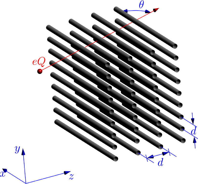
a)

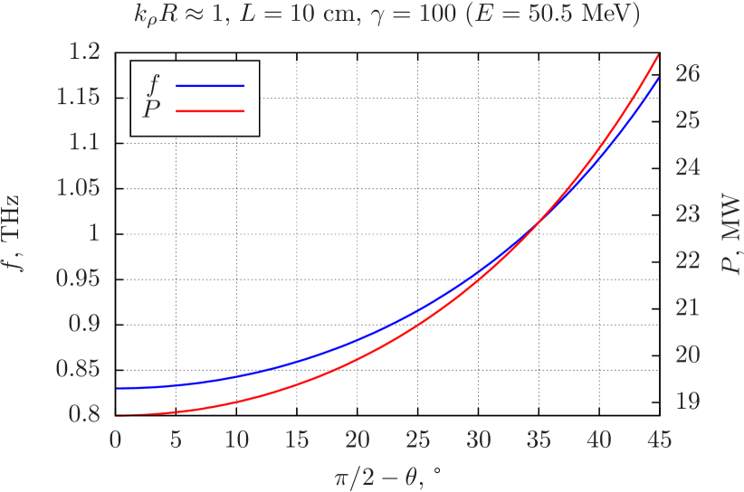
b)

Figure 13: The geometry of the problem (a) and dependencies of the parametric radiation frequency and power on the angle $\theta$ (b).

Until now we have considered only spontaneous radiation of electron bunches. However, the induced radiation can also occur when the electron beam moves through the crystal. The set of equations describing the interaction of an electromagnetic wave with the “crystal-beam” system, consists of Maxwell’s equations and those of particle motion in the electromagnetic field. By analyzing these equations in [43] expressions for generation threshold in case of two-wave diffraction were obtained. Dependencies of starting (necessary for the induced generation onset) currents for crystal built from metallic wires on the parameter $k_{\rho}R$ and on the crystal length $L$ (at $k_{\rho}R\sim 1$) calculated in accordance with [43] are presented below. The case of Bragg symmetric diffraction was considered. Lets point out that the starting current for $TE$-polarized wave is substantially lower than for $TM$-polarized wave. It is related to the fact that in first case $g_{0}>0$ (Cherenkov radiation is possible), while in second case $g_{0}<0$.

4 Conclusion

We have considered Cherenkov, transition and parametric (quasi-Cherenkov) radiation emitted by relativistic charged particles passing through a photonic crystal built from parallel metallic wires. The radiation emitted in the case when the wavelength becomes comparable with the wire radius and scattering by a single wire becomes anisotropic has been analyzed on the basis of the dynamical theory of diffraction in crystals made from anisotropically scattering centers. The dispersion equation derived in this paper enables finding the possible wave types in the crystal and calculating the unknown effective polarizabilities $g_{\tau}$ in the general case (at arbitrary values of scattering amplitudes $A(\varphi)$). We have also derived the expressions for spectral-angular distribution of parametric radiation in considered crystals.

Numerical solutions of the derived equations for the selected crystal geometry have confirmed the conclusion [5] that the intensity of radiation increases as the radius $R$ of wires is increased, attaining the maximum in the range $k_{\rho}R\sim 1$. It has been shown that a considerable contribution to the total intensity comes from a TE-polarized wave, but in the case when $k_{\rho}R\ll 1$, the radiation appears almost completely TM-polarized. The estimations made here show that at typical parameters of modern acceleration facilities, the radiation intensity attains rather high values, and so parametric radiation in a crystal built from metallic wires can be of interest for diverse practical applications, including the development of high-power THz pulse sources.

Appendix A Dispersion equation

The dispersion equation for a crystal made of parallel metallic wires that is valid for $0<k_{\rho}R\lesssim 1$, has the form

$$\det{D}=0,$$ (48)

where the elements of matrix $D$ are determined by the equalities

$$D_{11} =(\alpha B_{0}+C_{1})(iB^{\prime}_{1}+C_{7})+i(2\alpha C_{9}^{2}-\alpha C_{8}^{2}+\beta C_{8}C_{2})+(3\alpha C_{8}C_{9}-\beta C_{9}C_{2}),$$ (49)

$$D_{12} =-C_{3}(iB^{\prime}_{1}+C_{7})-i\beta C_{4}C_{8}+\beta C_{4}C_{9},$$

$$D_{13} =C_{2}(iB^{\prime}_{1}+C_{7})+\frac{i}{\beta}C_{8}(C_{1}-(1-\beta^{2})C_{5})-\frac{1}{\beta}C_{9}(C_{1}-(1-\beta^{2})C_{5})+\frac{\alpha}{\beta}B^{\prime}_{1}C_{9}-\frac{\alpha}{\beta}C_{8}C_{7},$$

$$D_{21} =-C_{3},$$

$$D_{22} =\frac{\alpha}{1-\beta^{2}}B_{1}+C_{5},$$

$$D_{23} =-C_{4},$$

$$D_{31} =\beta^{2}C_{2}(iB_{0}+C_{6})+i\beta C_{1}C_{8}-\beta C_{1}C_{9}-\alpha\beta C_{9}B_{0}-\alpha\beta C_{8}C_{6},$$

$$D_{32} =-\beta^{2}C_{4}(iB_{0}+C_{6})-i\beta C_{3}C_{8}+\beta C_{3}C_{9},$$

$$D_{33} =(\alpha B^{\prime}_{1}+C_{1}-C_{5}+\beta^{2}C_{5})(iB_{0}+C_{6})-i(2\alpha C_{9}^{2}-\alpha C_{8}^{2}-\beta C_{8}C_{2})-(3\alpha C_{8}C_{9}+\beta C_{9}C_{2}),$$

$\alpha=\frac{k_{z0}b}{2\pi}$, and $\beta=\frac{k_{y}}{k_{\rho}}$; $B_{0}$, $B_{1}$ and $B^{\prime}_{1}$ are expressed in terms of the amplitude of scattering by a wire as

$$B_{0} =\frac{1+i\pi A_{0}-S^{\prime}_{1}A_{0}}{A_{0}},$$ (50)

$$B_{1} =\frac{1+i\pi A_{1}/2-S^{\prime}_{3}A_{1}}{A_{1}},$$

$$B^{\prime}_{1} =\frac{1+i\pi A_{1}/2+(S^{\prime}_{3}-S^{\prime}_{1})A_{1}}{A_{1}}.$$

The sums $S^{\prime}_{n}$ and $C_{n}$ equal

$$S^{\prime}_{1} =2\left(\log\frac{k_{\rho}b}{4\pi}+C\right)-\sum\limits_{n\in\mathbb{N}_{1}}\frac{1}{|n|}+\sum\limits_{n\in\mathbb{N}_{2}}\left(\frac{2\pi}{\kappa_{n}b}-\frac{1}{|n|}\right),$$ (51)

$$S^{\prime}_{3} =\log\frac{k_{\rho}b}{4\pi}+C-\frac{1}{2}+\frac{2\pi^{2}+3k_{y}^{2}b^{2}}{3k_{\rho}^{2}b^{2}}+\frac{2\pi}{k_{\rho}b}\sum\limits_{n\in\mathbb{N}_{1}}\left(\frac{|k_{yn}|}{k_{\rho}}-\frac{k_{\rho}b}{4\pi|n|}\right)+\frac{2\pi}{k_{\rho}b}\sum\limits_{n\in\mathbb{N}_{2}}\left(\frac{|k_{yn}|}{k_{\rho}}-\frac{\kappa_{n}}{k_{\rho}}-\frac{k_{\rho}b}{4\pi|n|}\right),$$

$$C_{1} =-\frac{\sin k_{z}a}{\cos k_{z}a-\cos q_{z}a}-\sum\limits_{n\in\mathbb{N}_{1}}\frac{\sin k_{zn}a}{\cos k_{zn}a-\cos q_{z}a}\frac{k_{z}}{k_{zn}}-\sum\limits_{n\in\mathbb{N}_{2}}\left(-1+\frac{\sinh\kappa_{n}a}{\cosh\kappa_{n}a-\cos q_{z}a}\right)\frac{k_{z}}{\kappa_{n}},$$ (52)

$$C_{2} =-\frac{\sin k_{z}a}{\cos k_{z}a-\cos q_{z}a}-\sum\limits_{n\in\mathbb{N}_{1}}\frac{\sin k_{zn}a}{\cos k_{zn}a-\cos q_{z}a}\frac{k_{z}k_{yn}}{k_{zn}k_{y}}-\sum\limits_{n\in\mathbb{N}_{2}}\left(-1+\frac{\sinh\kappa_{n}a}{\cosh\kappa_{n}a-\cos q_{z}a}\right)\frac{k_{z}k_{yn}}{\kappa_{n}k_{y}},$$

$$C_{3} =\frac{\sin q_{z}a}{\cos k_{z}a-\cos q_{z}a}+\sum\limits_{n\in\mathbb{N}_{1}}\frac{\sin q_{z}a}{\cos k_{zn}a-\cos q_{z}a}+\sum\limits_{n\in\mathbb{N}_{2}}\frac{\sin q_{z}a}{\cosh\kappa_{n}a-\cos q_{z}a},$$

$$C_{4} =\frac{\sin q_{z}a}{\cos k_{z}a-\cos q_{z}a}+\sum\limits_{n\in\mathbb{N}_{1}}\frac{\sin q_{z}a}{\cos k_{zn}a-\cos q_{z}a}\frac{k_{yn}}{k_{y}}+\sum\limits_{n\in\mathbb{N}_{2}}\frac{\sin q_{z}a}{\cosh\kappa_{n}a-\cos q_{z}a}\frac{k_{yn}}{k_{y}},$$

$$C_{5} =-\frac{\sin k_{z}a}{\cos k_{z}a-\cos q_{z}a}-\sum\limits_{n\in\mathbb{N}_{1}}\frac{\sin k_{zn}a}{\cos k_{zn}a-\cos q_{z}a}\frac{k_{zn}}{k_{z}}+\sum\limits_{n\in\mathbb{N}_{2}}\left(-1+\frac{\sinh\kappa_{n}a}{\cosh\kappa_{n}a-\cos q_{z}a}\right)\frac{\kappa_{n}}{k_{z}},$$

$$C_{6} =\frac{2\pi}{k_{z}b}\left(1+\sum\limits_{n\in\mathbb{N}_{1}}\frac{k_{z}}{k_{zn}}\right),\;\;\;C_{7}=\frac{2\pi}{k_{z}b}\frac{k_{y}^{2}}{k_{\rho}^{2}}\left(1+\sum\limits_{n\in\mathbb{N}_{1}}\frac{k_{z}}{k_{zn}}\frac{k_{yn}^{2}}{k_{y}^{2}}\right),$$

$$C_{8} =-2\frac{k_{y}}{k_{\rho}}+\frac{2\pi}{k_{\rho}b}\sum\limits_{n\in\mathbb{N}_{2}}\frac{k_{yn}}{\kappa_{n}},\;\;\;C_{9}=\frac{2\pi}{k_{z}b}\frac{k_{y}}{k_{\rho}}\left(1+\sum\limits_{n\in\mathbb{N}_{1}}\frac{k_{z}}{k_{zn}}\frac{k_{yn}}{k_{y}}\right),$$

where $\kappa_{n}=\sqrt{k_{yn}^{2}-k_{\rho}^{2}}$, and summation is performed over the ranges $\mathbb{N}_{1}:\;N_{1}\leq n\leq N_{2},\;n\neq 0$, $\mathbb{N}_{2}:\;n\in(-\infty;N_{1})\cup(N_{2},+\infty)$, $N_{1}=\left[\frac{(k_{y}-k_{\rho})b}{2\pi}\right]$, and $N_{2}=\left[\frac{(k_{y}+k_{\rho})b}{2\pi}\right]$. Let us note that all sums appearing in (52) are real and their values are independent of the characteristics of the crystal-forming scattering elements (wires). The functions $S^{\prime}_{1}$, $S^{\prime}_{2}$, and $C_{6}$–$C_{9}$ are dependent only on the frequency and the direction of wave propagation (on $k_{y}$ and $k_{\rho}$) and on the crystal periods; besides that, the functions $C_{1}$–$C_{5}$ also depend on the $z$-component of the wave vector in the crystal $q_{z}$. If scattering by a single wire is elastic (which occurs for perfectly conducting wires), then $B_{0}$, $B_{1}$, and $B^{\prime}_{1}$ are purely real, which can be demonstrated using the optical theorem, see [20, 28]. It can be shown that in this case the solutions $q_{z}$ of the dispersion equation are also purely real (in the transmission band), i.e., no attenuation will occur for a wave in the crystal. If the wires have a finite conductivity, the solutions $q_{z}$ in the general case will be complex quantities.

Let us consider some cases when the dispersion simplifies appreciably. Let $k_{y}b=\pi m$, where $m\neq 0$ is the integer, i.e., the diffraction conditions in the crystal are fulfilled exactly for wave vectors $\mathbf{k}$, $\mathbf{k}+\boldsymbol{\tau}$, where reciprocal lattice vector $\boldsymbol{\tau}=\boldsymbol{\tau}_{y}=-\frac{2\pi m}{b}\mathbf{e}_{y}$. In this case, the sum $S_{2}=C_{8}+iC_{9}$ (see (21)) is identically equal to zero, and hence the coefficients $C_{8}$ and $C_{9}$ are also equal to zero. Moreover we can see that $C_{2}=C_{4}=0$. Under such conditions, the dispersion equation can be written in terms of real variables as follows:

$$(\alpha B^{\prime}_{1}+C_{1}-(1-\beta^{2})C_{5})\left((\alpha B_{0}+C_{1})(\alpha B_{1}+(1-\beta^{2})C_{5})-(1-\beta^{2})C_{3}^{2}\right)=0.$$ (53)

The approximate analytical solution of this equation for the simplest cases is found readily. Let, for example, $k_{x}=0$, $k_{y}=\pi/b$, $ka,kb<2\pi$, and $\varepsilon_{1}=\mu_{1}=1$, whereas for wave vectors $k$ and $q$ the condition $|q^{2}/k^{2}-1|\ll 1$ holds true. Then we have

$$C_{1}\approx C_{5}\approx-C_{3}\approx-\frac{4}{ka(q^{2}/k^{2}-1)}\frac{k_{z}}{k},$$ (54)

and after simple transformations the solutions of (53) can be presented in the form

$$\left\{\begin{aligned} \frac{q_{1}^{2}}{k^{2}}&=1+\frac{8\pi}{k^{2}\Omega_{2}}\left\{\frac{A_{0}}{1+i\pi A_{0}-S^{\prime}_{1}A_{0}}+\frac{A_{1}}{1+i\pi A_{1}/2-S^{\prime}_{3}A_{1}}\frac{k_{z}^{2}}{k^{2}}\right\},\\ \frac{q_{2}^{2}}{k^{2}}&=1+\frac{8\pi}{k^{2}\Omega_{2}}\frac{A_{1}}{1+i\pi A_{1}/2+(S^{\prime}_{3}-S^{\prime}_{1})A_{1}}\frac{k_{y}^{2}}{k^{2}}\end{aligned}\right.$$ (55)

On the other hand, in the case of two-wave dynamical diffraction the waves propagating in a photonic crystal are described by the following set of equations [5]:

$$\left\{\begin{aligned} &\left(\frac{\boldsymbol{q}^{2}}{k^{2}}-1-g^{s}_{0}\right)\mathbf{E}^{s}(\mathbf{q})-g^{s}_{-\boldsymbol{\tau}}\mathbf{E}^{s}(\mathbf{q}+\boldsymbol{\tau})=0,\\ &-g^{s}_{\boldsymbol{\tau}}\mathbf{E}^{s}(\mathbf{q})+\left(\frac{(\mathbf{q}+\boldsymbol{\tau})^{2}}{k^{2}}-1-g^{s}_{0}\right)\mathbf{E}^{s}(\mathbf{q}+\boldsymbol{\tau})=0,\end{aligned}\right.$$ (56)

where $\boldsymbol{\tau}$ is the reciprocal lattice vector, $\mathbf{q}$ is the wave vector in the crystal, the index $s$ numbers the two possible polarization states, $g_{\boldsymbol{\tau}}$ are the coefficients of expansion of the effective dielectric susceptibility of the crystal into the Foureir series in terms of reciprocal lattice vector:

$$\varepsilon(\mathbf{r})-1=\sum\limits_{\boldsymbol{\tau}}g_{\boldsymbol{\tau}}e^{i\boldsymbol{\tau}\mathbf{r}}.$$

The dispersion equation that follows from the system (56) has a simple form in the considered case of symmetric Laue diffraction:

$$(q^{2}-k^{2}(1+g_{0}))^{2}-k^{4}g_{\tau}^{2}=0.$$

It has the roots

$$\frac{q^{2}_{1,2}}{k^{2}}=1+g_{0}\pm g_{\tau}.$$

Comparing them with (55), we can find the unknown quantities $g_{0}$ and $g_{\tau}$. If the scattering amplitude is small, then we are led to the result that agrees well with the conclusions of [20]:

$$\left\{\begin{aligned} g_{0}&\approx\frac{4\pi}{k^{2}\Omega_{2}}\left\{\frac{A_{0}}{1+i\pi A_{0}}+\frac{A_{1}}{1+i\pi A_{1}/2}\right\},\\ g_{\tau}&\approx\frac{4\pi}{k^{2}\Omega_{2}}\left\{\frac{A_{0}}{1+i\pi A_{0}}+\frac{A_{1}}{1+i\pi A_{1}/2}\cos 2\theta_{B}\right\},\end{aligned}\right.$$ (57)

where $\cos 2\theta_{B}=\cos^{2}\theta_{B}-\sin^{2}\theta_{B}=\frac{k_{z}^{2}}{k^{2}}-\frac{k_{y}^{2}}{k^{2}}$.

The dispersion equation takes an even simpler form in the case of normal incidence of a wave onto the crystal ($k_{x}=k_{y}=0$). As $F^{\prime}_{1}$ here is identically zero (see (19)), then following the same lines of reasoning as in section 2.3, instead of the set of three equations (31) we come to a set of two equations (two first equations in (31), where we assume $F^{\prime}_{1n}=0$). In terms of notation (49), the condition of vanishing the determinant of the system can be written in the form

$$D_{11}D_{22}-D_{12}D_{21}=0.$$ (58)

Taking into account that here the coefficients $C_{8}=C_{9}=0$, as well as in the considered case of diffraction, we can write the explicit form of the dispersion equation:

$$\frac{k_{1}b}{2\pi}=-\frac{C_{1}A_{0}}{1+i\pi A_{0}-S^{\prime}_{1}A_{0}}-\frac{C_{5}A_{1}}{1+i\pi A_{1}/2-S^{\prime}_{3}A_{1}}+\frac{2\pi}{k_{1}b}\frac{(C_{3}^{2}-C_{1}C_{5})A_{0}A_{1}}{(1+i\pi A_{0}-S^{\prime}_{1}A_{0})(1+i\pi A_{1}/2-S^{\prime}_{3}A_{1})}.$$ (59)

References

- [1] V. Baryshevsky, I. Feranchuk, and A. Ulyanenkov, Parametric X-Ray Radiation in Crystals: Theory, Experiment and Applications. Springer, 2005.
- [2] V. Baryshevsky and A. Gurinovich, “Spontaneous and induced parametric and smith-purcell radiation from electrons moving in a photonic crystal built from the metallic threads,” Nuclear Inst. and Meth. B, vol. 252, no. 1, pp. 92 – 101, 2006.
- [3] V. Baryshevsky and E. Gurnevich, “The possibility of cherenkov radiation generation in a photonic crystal formed by parallel metallic threads,” Vestnik BSU (The Journal of the Belarusian State University), ser. 1, No.3, no. 3, pp. 38–44, 2009.
- [4] V. Baryshevsky and E. Gurnevich, “The possibility of cherenkov radiation generation in a photonic crystal formed by parallel metallic threads,” Proc. Of 2010 Intern. Kharkov Symp. on Phys. and Engineering of Microwaves, Milimeter and Submilimeter Waves (MSMW10), 21-26 June 2010, pp. 1 – 3, 2010.
- [5] V. Baryshevsky and A. Gurinovich, “Quasi-cherenkov parametric radiation from relativistic particles passing through a photonic crystal,” Nucl. Inst. and Meth. B, vol. 355, pp. 69 – 75, 2015. LANL e-print arXiv:1406.2126.
- [6] V. Vorobev and A. Tyukhtin, “Nondivergent cherenkov radiation in a wire metamaterial,” Phys. Rev. Lett., vol. 108, p. 184801, 2012.
- [7] D. Shiffler, J. Luginsland, D. French, and J. Watrous, “A cerenkov-like maser based on a metamaterial structure,” IEEE Trans. on Plasma Sci., vol. 38, no. 6, pp. 1462 – 1465, 2010.
- [8] S. J. Smith and E. M. Purcell, “Visible light from localized surface charges moving across a grating,” Phys. Rev., vol. 92, pp. 1069–1069, 1953.
- [9] B. Bolotovskii and G. Voskresenskii, “Diffraction radiation,” Sov. Phys. Usp., vol. 9, no. 1, p. 73, 1966.
- [10] M. Ter-Mikaelian, “Emission of fast particles in a heterogeneous medium,” Doklady Akademii Nauk SSSR, vol. 34, p. 318, 1960.
- [11] M. Ter-Mikaelyan, “Emission of fast particles in a heterogeneous medium,” Nuclear Physics, vol. 24, pp. 43–61, jan 1961.
- [12] V. Baryshevsky and P. Molchanov, “Volume free electron laser with a” grid” photonic crystal in a cylindrical waveguide,” Acta Physica Polonica-Series A General Physics, vol. 115, no. 6, p. 971, 2009.
- [13] V. Baryshevsky, N. Belous, A. Gurinovich, E. Gurnevich, V. Evdokimov, and P. Molchanov, “Volume free electron laser with a ”grid” photonic crystal with variable period: Theory and experiment,” in Proceedings of FEL2009, Liverpool, UK, 2009.
- [14] V. Baryshevsky, N. Belous, A. Gurinovich, A. Lobko, P. Molchanov, and V. Stolyarsky, “Experimental study of a volume free electron laser with a “grid” resonator,” Proc. of FEL 2006 BESSY, Berlin, Germany, pp. 331 – 334, 2006.
- [15] A. Tyukhtin and V. Vorobev, “Cherenkov radiation in a metamaterial comprised of coated wires,” Journal of the Optical Society of America B, vol. 30, p. 1524, may 2013.
- [16] A. Tyukhtin and V. Vorobev, “Radiation of charges moving along the boundary of a wire metamaterial,” Physical Review E, vol. 89, jan 2014.
- [17] V. Vorobev and A. Tyukhtin, “Radiation of a charge moving in wire metamaterial perpendicularly to the main axis,” J. Phys.: Conf. Ser., vol. 357, p. 012006, may 2012.
- [18] A. Tyukhtin, V. Vorobev, and S. Galyamin, “Radiation excited by a charged-particle bunch on a planar periodic wire structure,” Phys. Rev. ST Accel. Beams, vol. 17, dec 2014.
- [19] C. Simovski, P. Belov, A. Atrashchenko, and Y. Kivshar, “Wire metamaterials: Physics and applications,” Advanced Materials, vol. 24, no. 31, pp. 4229 – 4248, 2012.
- [20] V. Baryshevsky and E. Gurnevich, “Dynamical diffraction theory of waves in photonic crystals built from anisotropically scattering elements,” Journal of Nanophotonics, vol. 6, no. 1, p. 061713, 2012.
- [21] V. G. Baryshevsky, High-energy nuclear optics of polarized particles. World Scientific, 2012.
- [22] V. Baryshevsky, “Parametric x-ray radiation at a small angle near the velocity direction of the relativistic particle,” Nucl. Inst. and Meth. B, vol. 122, no. 1, pp. 13 – 18, 1997.
- [23] P. M. Morse and H. Feshbach, Methods of Theoretical Physics. Mc Graw Hill, New York, 1953.
- [24] V. Nikolskiy and T. Nikolskaya, Electrodynamics and Radio Waves Propagation [in Russian]. Nauka, Moscow, 1989.
- [25] M. Silveirinha, “Nonlocal homogenization model for a periodic array of -negative rods,” Phys. Rev. E, vol. 73, p. 046612, Apr 2006.
- [26] J. Wait, “Scattering of a plane wave from a circular dielectric cylinder at oblique incidence,” Canadian Journal of Physics, vol. 33, no. 5, pp. 189–195, 1955.
- [27] E. Jahnke, F. Emde, and F. Lösch, Tables of Higher Functions. B.G. Teubner, Stuttgart, 1966.
- [28] L. Landau and E. Lifshitz, Quantum Mechanics: Non-Relativistic Theory. Pergamon Press, 1977.
- [29] Z. Pinsker, Dynamical Scattering of X-Rays in Crystals. Springer-Verlag, Berlin, 1978.
- [30] P. P. Ewald, ed., Fifty Years of X-Ray Diffraction. Springer Science + Business Media, Utrecht, 1962.
- [31] R. James, The Optical Principles of the Diffraction of X-Rays. G. Bell & Sons, London, 1948.
- [32] V. Baryshevsky and E. Gurnevich, “Multiple scattering of waves in 3d crystals (natural or photonic) formed by anisotropically scattering centers,” LANL preprint arXiv:1307.1544, 2013.
- [33] P. A. Belov, S. A. Tretyakov, and A. J. Viitanen, “Dispersion and reflection properties of artificial media formed by regular lattices of ideally conducting wires,” J. of Electromagn. Waves and Appl., vol. 16, no. 8, pp. 1153–1170, 2002.
- [34] V. M. Agranovich and V. Ginzburg, Crystal Optics with Spatial Dispersion, and Excitons. Springer Berlin Heidelberg, 1984.
- [35] O. Lundh, J. Lim, C. Rechatin, L. Ammoura, A. Ben-Ismail, X. Davoine, G. Gallot, J. Goddet, E. Lefebvre, V. Malka, et al., “Few femtosecond, few kiloampere electron bunch produced by a laser-plasma accelerator,” Nature Physics, vol. 7, no. 3, pp. 219 – 222, 2011.
- [36] Y. Liu, X. Wang, D. Cline, M. Babzien, J. Fang, J. Gallardo, K. Kusche, I. Pogorelsky, J. Skaritka, and A. Van Steenbergen, “Experimental observation of femtosecond electron beam microbunching by inverse free-electron-laser acceleration,” Phys. Rev. Lett., vol. 80, no. 20, p. 4418, 1998.
- [37] K. Kan, J. Yang, T. Kondoh, K. Norizawa, A. Ogata, T. Kozawa, and Y. Yoshida, “Femtosecond electron bunch generation using photocathode rf gun,” Proc. of the FEL2010 Conf., Malmo, Sweden, pp. 366 – 369, 2010.
- [38] V. Baryshevsky, “Spontaneous and induced radiation by relativistic particles in natural and photonic crystals. crystal x-ray lasers and volume free electron lasers (vfel),” arXiv preprint arXiv:1101.0783, 2011.
- [39] V. G. Baryshevsky, “Spontaneous and induced radiation by electrons/positrons in natural and photonic crystals. volume free electron lasers (VFELs): From microwave and optical to x-ray range,” Nucl. Instrum. Methods Phys. Res., Sect. B, vol. 355, pp. 17–23, jul 2015.
- [40] R. Ganter, “Swissfel-conceptual design report,” tech. rep., Paul Scherrer Institute (PSI), 2010.
- [41] V. G. Baryshevsky and I. D. Feranchuk, “Parametric x-rays from ultrarelativistic electrons in a crystal: theory and possibilities of practical utilization,” J. Phys. France, vol. 44, no. 8, pp. 913–922, 1983.
- [42] V. Baryshevsky and E. Gurnevich, “Quasi-cherenkov radiation in a photonic crystal built from parallel metallic wires in the case of anisotropic scattering of waves by the wire,” in Nonlinear Dynamics and Applications (Proc. of NPCS-2015 Conf., Minsk, Belarus), vol. 21, pp. 126–138, 2015.
- [43] V. Baryshevsky, K. Batrakov, and I. Dubovskaya, “Parametric(quasi-cerenkov) x-ray free electron lasers,” Journal of Physics D. Applied Physics, vol. 24, pp. 1250–7, 1991.