Online Output-Feedback Parameter and State Estimation for Second Order Linear Systems

Abstract

In this paper, a concurrent learning based adaptive observer is developed for a class of second-order linear time-invariant systems with uncertain system matrices. The developed technique yields an exponentially convergent state estimator and an exponentially convergent parameter estimator. As opposed to persistent excitation required for parameter convergence in traditional adaptive methods, excitation over a finite time-interval is sufficient for the developed technique to achieve exponential convergence. Simulation results in both noise-free and noisy environments are presented to validate the design.

I Introduction

Over the the past decade, the role of autonomy in everyday life has seen an unprecedented growth. As a result, the tasks performed by autonomous systems have also grown in complexity. Adaptive control methods have emerged as a tool to address a subset of the challenges posed by complexity. In particular, autonomous systems typically operate in uncertain and changing environments. The ability to learn the uncertainty and to adapt to changes is thus an integral part of a modern control system.

Traditional adaptive control methods handle uncertainty in the system dynamics by maintaining a parametric estimate of the model and utilizing it to generate a feedforward control signal [1, 2, 3]. While the feedforward-feedback architecture guarantees stability of the closed-loop, the control law is not robust to disturbances, and seldom provides information regarding the quality of the estimated model [1, 2]. In addition to system identification, parameter convergence in adaptive control schemes provides increased robustness and improved transient performance (cf. [4, 5, 6]). Modifications such as $\sigma-$modification (cf. [1, Section 8.4.1]) and $e-$modification (cf. [7]) result in robust adaptive controllers, however, the parameter estimates generally do not converge to the true values of the corresponding parameters [8, 7, 2, 1, 9]. The parameters can be shown to converge under persistent excitation; however, in addition to the control effort required to maintain excitation, persistent excitation can lead to mechanical fatigue, and often directly conflicts with control objectives such as regulation and tracking.

Recently, a novel data-driven concurrent learning (CL) adaptive control method that achieves parameter convergence under a finite excitation condition was developed in results such as [6, 10, 11]. In CL adaptive control, parameter convergence is achieved by storing data during time-intervals when the system is excited, and then utilizing the stored data to drive adaptation when excitation is unavailable. Since excitation is required only over a finite time-interval, energy utilization and mechanical fatigue can be kept to a minimum, and asymptotic objectives such as regulation and tracking can be effectively achieved. Furthermore, CL adaptive control methods possess similar robustness to bounded disturbances as $\sigma-$modification, $e-$modification, etc, without the associated drawbacks such as drawing the parameter estimates to arbitrary set-points [6, 10, 12, 11].

Adaptation techniques similar to the CL method were utilized to implement reinforcement learning under finite excitation conditions in results such as [13, 14, 15, 16, 17, 18]. CL methods have also been extended to classes of switched systems (cf. [19]) and systems driven by stochastic processes (cf. [20]). A major drawback of CL methods is that they require numerical differentiation of the state measurements. CL methods that do not require numerical differentiation of the state measurements are developed in results such as [21] and [22], however, they require full state feedback. Since full state feedback is often not available, the development of an output-feedback CL framework is well-motivated.

In this paper, a CL-based adaptive observer is developed for a class of second-order linear time-invariant systems. The elements of the system matrices are assumed to be uncertain and the dimensions of the matrices are assumed to be known. The developed technique yields an exponentially convergent state estimator and an exponentially convergent parameter estimator. Excitation over a finite time-interval (as opposed to persistent excitation) is required for exponential convergence. Simulation results are provided in a noise-free environment to validate the design. Simulation results with added measurement noise are also provided to demonstrate robustness to sensor noise.

In the following, a linear error system is developed in Section II to facilitate CL-based adaptation. A CL-based parameter estimator is designed in Section III. A state-observer that utilizes the parameter estimates to estimate the generalized velocity is developed in Section IV. A Lyapunov-based stability analysis of the parameter estimator and the state observer is presented in Section V. Section VI presents numerical simulation results, and Section VII presents concluding remarks and a few comments on possible extensions of the developed technique.

II Error System for Estimation

Consider a second order linear system of the form

$$\dot{p}\left(t\right) =q\left(t\right),$$

$$\dot{q}\left(t\right) =Ax\left(t\right)+Bu\left(t\right),$$

$$y\left(t\right) =p\left(t\right),$$ (1)

where $p:\mathbb{R}_{\geq t_{0}}\to\mathbb{R}^{n}$ and $q:\mathbb{R}_{\geq t_{0}}\to\mathbb{R}^{n}$ denote the generalized position states and the generalized velocity states, respectively, $x\triangleq\begin{bmatrix}p^{T}&q^{T}\end{bmatrix}^{T}$ is the system state, $A\in\mathbb{R}^{n\times 2n}$ and $B\in\mathbb{R}^{n\times m}$ denote the system matrices, and $y:\mathbb{R}_{\geq t_{0}}\to\mathbb{R}^{n}$ denotes the output. The objective is to design an adaptive estimator to identify the unknown matrices $A$ and $B$, online, using input-output measurements. It is assumed that the system is controlled using a stabilizing input, i.e., $x,\>u\in\mathcal{L}_{\infty}$. Systems of the form (1) can be obtained through linearization of second-order Euler-Lagrange models, and hence, represent a wide class of physical plants, including but not limited to robotic manipulators and autonomous ground, aerial, and underwater vehicles.

To obtain an error signal for parameter identification, the system in (1) is expressed in the form

$$\dot{q}\left(t\right)=A_{1}p\left(t\right)+A_{2}q\left(t\right)+Bu\left(t\right),$$ (2)

where $A_{1}\in\mathbb{R}^{n\times n}$ and $A_{2}\in\mathbb{R}^{n\times n}$ are constant matrices such that $A=\begin{bmatrix}A_{1}&A_{2}\end{bmatrix}$. Integrating (2) over the interval $\left[t-T_{1},t\right]$ for some constant $T_{1}\in\mathbb{R}_{>0}$,

$$q\left(t\right)-q\left(t-T_{1}\right)=A_{1}\intop_{t-T_{1}}^{t}p\left(\tau\right)\textnormal{d}\tau+A_{2}\intop_{t-T_{1}}^{t}q\left(\tau\right)\textnormal{d}\tau\\ +B\intop_{t-T_{1}}^{t}u\left(\tau\right)\textnormal{d}\tau.$$ (3)

Integrating again over the interval $\left[t-T_{2},t\right]$ for some constant $T_{2}\in\mathbb{R}_{>0}$,

$$\intop_{t-T_{2}}^{t}\left(q\left(\sigma\right)-q\left(\sigma-T_{1}\right)\right)\textnormal{d}\sigma=A_{1}\intop_{t-T_{2}}^{t}\intop_{\sigma-T_{1}}^{\sigma}p\left(\tau\right)\textnormal{d}\tau\textnormal{d}\sigma\\ +A_{2}\intop_{t-T_{2}}^{t}\intop_{\sigma-T_{1}}^{\sigma}q\left(\tau\right)\textnormal{d}\tau\textnormal{d}\sigma+B\intop_{t-T_{2}}^{t}\intop_{\sigma-T_{1}}^{\sigma}u\left(\tau\right)\textnormal{d}\tau\textnormal{d}\sigma.$$ (4)

Using the Fundamental Theorem of Calculus and the fact that $q\left(t\right)=\dot{p}\left(t\right)$,

$$p\left(t\right)-p\left(t-T_{2}\right)-p\left(t-T_{1}\right)+p\left(t-T_{2}-T_{1}\right)=\\ A_{1}F\left(t\right)+A_{2}G\left(t\right)+BU\left(t\right).$$ (5)

where

$$F\left(t\right)\triangleq\begin{cases}\intop_{t-T_{2}}^{t}\intop_{\sigma-T_{1}}^{\sigma}p\left(\tau\right)\textnormal{d}\tau\textnormal{d}\sigma,&t\in\left[t_{0}+T_{1}+T_{2},\infty\right),\\ 0,&t<t_{0}+T_{1}+T_{2},\end{cases}$$ (6)

$$G\left(t\right)\!\triangleq\!\begin{cases}\!\intop_{t-T_{2}}^{t}\!\!\left(p\left(\!\sigma\!\right)\!-\!p\left(\sigma\!-\!T_{1}\right)\!\right)\textnormal{d}\sigma,&t\!\in\!\left[t_{0}\!+\!T_{1}\!+\!T_{2},\infty\!\right),\\ 0&t<t_{0}+T_{1}+T_{2},\end{cases}$$ (7)

and

$$U\left(t\right)\triangleq\begin{cases}\intop_{t-T_{2}}^{t}\intop_{\sigma-T_{1}}^{\sigma}u\left(\tau\right)\textnormal{d}\tau\textnormal{d}\sigma,&t\in\left[t_{0}+T_{1}+T_{2},\infty\right),\\ 0&t<t_{0}+T_{1}+T_{2}.\end{cases}$$ (8)

The utility of the integral form in (5) is that it is independent of the generalized velocity states, $q$. The expression in (5) can be rearranged to form the linear error system

$$\mathcal{F}\left(t\right)=\mathcal{G}\left(t\right)\theta,\>\forall t\in\mathbb{R}_{\geq t_{0}}.$$ (9)

In (9), $\theta$ is a vector of unknown parameters, defined as $\theta\triangleq\begin{bmatrix}\operatorname{vec}\left(A_{1}\right)^{T}&\operatorname{vec}\left(A_{2}\right)^{T}&\operatorname{vec}\left(B\right)^{T}\end{bmatrix}^{T}\in\mathbb{R}^{2n^{2}+mn}$, where $\operatorname{vec}\left(\cdot\right)$ denotes the vectorization operator and the matrices $\mathcal{F}:\mathbb{R}_{\geq 0}\to\mathbb{R}^{n}$ and $\mathcal{G}:\mathbb{R}_{\geq 0}\to\mathbb{R}^{n\times 2n^{2}+mn}$ are defined as

$$\mathcal{F}\left(t\right) \triangleq\begin{cases}\begin{gathered}p\left(t\!-\!T_{2}\!-\!T_{1}\right)\!-\!p\left(t\!-\!T_{1}\right)\\ \!+p\left(t\right)\!-\!p\left(t\!-\!T_{2}\right),\end{gathered}&t\!\in\!\left[t_{0}\!+\!T_{1}\!+\!T_{2},\infty\right),\\ 0&t<t_{0}+T_{1}+T_{2}.\end{cases}$$

$$\mathcal{G}\left(t\right) \triangleq\begin{bmatrix}\left(F\left(t\right)\varotimes\operatorname{I}_{n}\right)^{T}&\left(G\left(t\right)\varotimes\operatorname{I}_{n}\right)^{T}&\left(U\left(t\right)\varotimes\operatorname{I}_{n}\right)^{T}\end{bmatrix},$$

where $\operatorname{I}_{n}$ denotes an $n\times n$ identity matrix, and $\varotimes$ denotes the Kronecker product. Note that even though the linear relationship in (9) is valid for all $t\in\mathbb{R}_{\geq t_{0}},$ it provides useful information about the vector $\theta$ only after $t\geq t_{0}+T_{1}+T_{2}$.

The linear error system in (9) motivates the adaptive estimation scheme that follows. The design is inspired by the concurrent learning (cf. [23]) technique. Concurrent learning enables parameter convergence in adaptive control by using stored data to update the parameter estimates. Traditionally, adaptive control methods guarantee parameter convergence only if the appropriate PE conditions are met (cf. [1, Chapter 4]). Concurrent learning uses stored data to soften the PE condition to an excitation condition over a finite time-interval. Concurrent learning methods such as [6] and [11] require numerical differentiation of the system state, and concurrent learning techniques such as [22] and [21] require full state measurements. In the following, a concurrent learning method that utilizes only the output measurements is developed.

III Parameter Estimator Design

To obtain output-feedback concurrent learning update law for the parameter estimates, a history stack denoted by $\mathcal{H}$ is utilized. The history stack is a set of ordered pairs $\left\{\left(\mathcal{F}_{i},\mathcal{G}_{i}\right)\right\}_{i=1}^{M}$ such that

$$\mathcal{F}_{i}=\mathcal{G}_{i}\theta,\>\forall i\in\left\{1,\cdots,M\right\}.$$ (10)

If a history stack that satisfies (11) is not available a priori, it can be recorded online, using the relationship in (9), by selecting a set of time-instances $\left\{t_{i}\right\}_{i=1}^{M}$ and letting

$$\mathcal{F}_{i} =\mathcal{F}\left(t_{i}\right),$$

$$\mathcal{G}_{i} =\mathcal{G}\left(t_{i}\right).$$ (11)

Furthermore, a singular value maximization algorithm is used to select the time instances $\left\{t_{i}\right\}_{i=1}^{M}$. That is, a data-point $\left\{\left(\mathcal{F}_{j},\mathcal{G}_{j}\right)\right\}$ in the history stack is replaced by a new data-point $\left\{\left(\mathcal{F}^{*},\mathcal{G}^{*}\right)\right\}$, where $\mathcal{F}^{*}=\mathcal{F}\left(t\right)$ and $\mathcal{G}^{*}=\mathcal{G}\left(t\right)$, for some $t$, only if

$$\lambda_{\min}\!\left\{\!\sum_{i\neq j}\mathcal{G}_{i}^{T}\mathcal{G}_{i}\!+\!\mathcal{G}_{j}^{T}\mathcal{G}_{j}\!\right\}\!<\!\lambda_{\min}\!\left\{\!\sum_{i\neq j}\mathcal{G}_{i}^{T}\mathcal{G}_{i}\!+\!\mathcal{G}^{*T}\mathcal{G}^{*}\!\right\},$$

where $\lambda_{\min}\left\{\cdot\right\}$ denotes the minimum Eigenvalue of a matrix.

Definition 1.

A history stack $\left\{\left(\mathcal{F}_{i},\mathcal{G}_{i}\right)\right\}_{i=1}^{M}$ is called full rank if there exists a constant $\underline{c}\in\mathbb{R}$ such that

$$0<\underline{c}<\lambda_{\min}\left\{\mathscr{G}\right\},$$ (12)

where the matrix $\mathscr{G}\in\mathbb{R}^{\left(2n^{2}+mn\right)\times\left(2n^{2}+mn\right)}$ is defined as $\mathscr{G}\triangleq\sum_{i=1}^{M}\mathcal{G}_{i}^{T}\mathcal{G}_{i}$.

The concurrent learning update law to estimate the unknown parameters is then given by

$$\dot{\hat{\theta}}\left(t\right)=k_{\theta}\Gamma\left(t\right)\sum_{i=1}^{M}\mathcal{G}_{i}^{T}\left(\mathcal{F}_{i}-\mathcal{G}_{i}\hat{\theta}\left(t\right)\right),$$ (13)

where $k_{\theta}\in\mathbb{R}_{>0}$ is a constant adaptation gain and $\Gamma:\mathbb{R}_{\geq 0}\to\mathbb{R}^{\left(2n^{2}+mn\right)\times\left(2n^{2}+mn\right)}$ is the least-squares gain updated using the update law

$$\dot{\Gamma}\left(t\right)=\beta_{1}\Gamma\left(t\right)-k_{\theta}\Gamma\left(t\right)\sum_{i=1}^{M}\mathcal{G}_{i}^{T}\mathcal{G}_{i}\Gamma\left(t\right).$$ (14)

Using arguments similar to Corollary 4.3.2 in [1], it can be shown that provided $\lambda_{\min}\left\{\Gamma^{-1}\left(t_{0}\right)\right\}>0$, the least squares gain matrix satisfies

$$\underline{\Gamma}\operatorname{I}_{\left(2n^{2}+mn\right)}\leq\Gamma\left(t\right)\leq\overline{\Gamma}\operatorname{I}_{\left(2n^{2}+mn\right)},$$ (15)

where $\underline{\Gamma}$ and $\overline{\Gamma}$ are positive constants, and $\operatorname{I}_{n}$ denotes an $n\times n$ identity matrix. The following finite-excitation assumption is necessary for the update law in (13) to result in an exponentially convergent parameter estimator.

Assumption 1.

For a given $M\in\mathbb{N}$ and $\underline{c}\in\mathbb{R}_{>0}$, there exists a set of time instances $\left\{t_{i}\right\}_{i=1}^{M}$ such that a history stack recorded using (11) is full rank.

Since the history stack is updated using a singular value maximization algorithm, the matrix $\mathscr{G}$ is a piece-wise constant function of time. The use of singular value maximization to update the history stack implies that once the matrix $\mathscr{G}$ satisfies (12), at some $t=T$, and for some $\underline{c}$, the condition $\underline{c}<\lambda_{\min}\left\{\mathscr{G}\left(t\right)\right\}$ holds for all $t\geq T$. The following section details the design of an exponentially convergent adaptive state-observer.

IV State Observer Design

To facilitate parameter estimation based on a prediction error, a state observer is developed in the following. To facilitate the design, the dynamics in (1) are expressed in the form

$$\dot{p}\left(t\right) =q\left(t\right),$$

$$\dot{q}\left(t\right) =Y\left(x\left(t\right),u\left(t\right)\right)\theta,$$

where $Y:\mathbb{R}^{n}\times\mathbb{R}^{m}\to\mathbb{R}^{n\times\left(2n^{2}+mn\right)}$ is defined as $Y\left(x,u\right)=\begin{bmatrix}\left(p\varotimes\operatorname{I}_{n}\right)^{T}&\left(q\varotimes\operatorname{I}_{n}\right)^{T}&\left(u\varotimes\operatorname{I}_{n}\right)^{T}\end{bmatrix}.$ The adaptive state observer is then designed as

$$\dot{\hat{p}}\left(t\right) =\hat{q}\left(t\right),\quad\hat{p}\left(t_{0}\right)=p\left(t_{0}\right),$$

$$\dot{\hat{q}}\left(t\right) =Y\left(x\left(t\right),u\left(t\right)\right)\hat{\theta}\left(t\right)+\nu\left(t\right),\quad\hat{q}\left(t_{0}\right)=0,$$ (16)

where $\hat{p}:\mathbb{R}_{\geq t_{0}}\to\mathbb{R}^{n}$, $\hat{q}:\mathbb{R}_{\geq t_{0}}\to\mathbb{R}^{n}$, $\hat{x}:\mathbb{R}_{\geq t_{0}}\to\mathbb{R}^{n}$, and $\hat{\theta}:\mathbb{R}_{\geq t_{0}}\to\mathbb{R}^{n}$ are estimates of $p$, $q$, $x$, and $\theta$, respectively, $\nu$ is the feedback component of the identifier, to be designed later, and the prediction error $\tilde{p}:\mathbb{R}_{\geq t_{0}}\to\mathbb{R}^{n}$ is defined as

$$\tilde{p}\left(t\right)=p\left(t\right)-\hat{p}\left(t\right).$$

The update law for the generalized velocity estimate depends on the entire state $x$. However, using the structure of the matrix $Y$ and integrating by parts, the observer can be implemented without using generalized velocity measurements. Consider the integral form of (16)

$$\hat{q}\left(t\right)-\hat{q}\left(t_{0}\right)=\intop_{t_{0}}^{t}\left(Y\left(x\left(\tau\right),u\left(\tau\right)\right)\hat{\theta}\left(\tau\right)+\nu\left(\tau\right)\right)\textnormal{d}\tau.$$

Using the definition of $Y$ and $\theta$, and expanding the integral,

$$\hat{q}\left(t\right)-\hat{q}\left(t_{0}\right)=\intop_{t_{0}}^{t}\left(p\left(\tau\right)\varotimes\operatorname{I}_{n}\right)^{T}\operatorname{vec}\left(\hat{A}_{1}\left(\tau\right)\right)\textnormal{d}\tau\\ +\intop_{t_{0}}^{t}\left(u\left(\tau\right)\varotimes\operatorname{I}_{n}\right)^{T}\operatorname{vec}\left(\hat{B}\left(\tau\right)\right)\textnormal{d}\tau+\intop_{t_{0}}^{t}\nu\left(\tau\right)\textnormal{d}\tau\\ +\intop_{t_{0}}^{t}\left(q\left(\tau\right)\varotimes\operatorname{I}_{n}\right)^{T}\operatorname{vec}\left(\hat{A}_{2}\left(\tau\right)\right)\textnormal{d}\tau.$$

The last term of the integral can be further expanded using integration by parts to yield

$$\intop_{t_{0}}^{t}\left(q\left(\tau\right)\varotimes\operatorname{I}_{n}\right)^{T}\operatorname{vec}\left(\hat{A}_{2}\left(\tau\right)\right)\textnormal{d}\tau=\\ \left(p\left(t\right)\varotimes\operatorname{I}_{n}\right)^{T}\operatorname{vec}\left(\hat{A}_{2}\left(t\right)\right)-\left(p\left(t_{0}\right)\varotimes\operatorname{I}_{n}\right)^{T}\operatorname{vec}\left(\hat{A}_{2}\left(t_{0}\right)\right)\\ -\intop_{t_{0}}^{t}\left(p\left(\tau\right)\varotimes\operatorname{I}_{n}\right)^{T}\operatorname{vec}\left(\dot{\hat{A}}_{2}\left(\tau\right)\right)\textnormal{d}\tau.$$

Thus, the update law in (16) can be implemented without generalized velocity measurements as

$$\hat{q}\left(t\right)=\intop_{t_{0}}^{t}\left(u\left(\tau\right)\varotimes\operatorname{I}_{n}\right)^{T}\operatorname{vec}\left(\hat{B}\left(\tau\right)\right)\textnormal{d}\tau+\intop_{t_{0}}^{t}\nu\left(\tau\right)\textnormal{d}\tau\\ +\hat{q}\left(t_{0}\right)+\intop_{t_{0}}^{t}\!\!\left(p\left(\tau\right)\varotimes\operatorname{I}_{n}\right)^{T}\!\!\left(\!\operatorname{vec}\left(\hat{A}_{1}\left(\tau\right)\right)\!-\!\operatorname{vec}\left(\dot{\hat{A}}_{2}\left(\tau\right)\right)\!\right)\textnormal{d}\tau\\ +\left(p\left(t\right)\varotimes\operatorname{I}_{n}\right)^{T}\operatorname{vec}\left(\hat{A}_{2}\left(t\right)\right)-\left(p\left(t_{0}\right)\varotimes\operatorname{I}_{n}\right)^{T}\operatorname{vec}\left(\hat{A}_{2}\left(t_{0}\right)\right)$$ (17)

To facilitate the design of the feedback component $\nu$, let

$$r\left(t\right)=\tilde{q}\left(t\right)+\alpha\tilde{p}\left(t\right)+\eta\left(t\right),$$ (18)

where the signal $\eta$ is added to compensate for the fact that the generalized velocity state, $q$, is not measurable. Based on the subsequent stability analysis, the signal $\eta$ is designed as the output of the dynamic filter

$$\dot{\eta}\left(t\right) =-\beta\eta\left(t\right)-kr\left(t\right)-\alpha\tilde{q}\left(t\right),\quad\eta\left(t_{0}\right)=0,$$ (19)

and the feedback component $\nu$ is designed as

$$\nu\left(t\right)=\tilde{p}\left(t\right)-\left(k+\alpha+\beta\right)\eta\left(t\right).$$ (20)

The design of the signals $\eta$ and $\nu$ to estimate the state from output measurements is inspired by the $p-$filter (cf. [24]). Similar to the update law for the generalized velocity, using the the fact that $\tilde{p}\left(t_{0}\right)=0$, the signal $\eta$ can be implemented using the integral form

$$\eta\left(t\right)=-\intop_{t_{0}}^{t}\left(\beta+k\right)\eta\left(\tau\right)\textnormal{d}\tau-\intop_{t_{0}}^{t}k\alpha\tilde{p}\left(\tau\right)\textnormal{d}\tau-\left(k+\alpha\right)\tilde{p}\left(t\right).$$ (21)

A Lyapunov-based analysis of the parameter and the state estimation errors is presented in the following section.

V Stability Analysis

To facilitate the analysis, (10) and (13) are used to express the dynamics of the parameter estimation error as

$$\dot{\tilde{\theta}}\left(t\right)=-k_{\theta}\Gamma\left(t\right)\mathscr{G}\left(t\right)\tilde{\theta}\left(t\right).$$ (22)

Since the function $\mathscr{G}:\mathbb{R}_{\geq t_{0}}\to\mathbb{R}^{\left(2n^{2}+mn\right)\times\left(2n^{2}+mn\right)}$ is piece-wise continuous, the trajectories of (22), and of all the subsequent error systems involving $\mathscr{G}$, are defined in the sense of Carathéodory. Using the dynamics in (1), (16), (19), and the design of the feedback component in (20), the time-derivative of the error signal $r$ is given by

$$\dot{r}\left(t\right)=Y\left(x\left(t\right),u\left(t\right)\right)\tilde{\theta}\left(t\right)-\tilde{p}\left(t\right)+\left(k+\alpha\right)\eta\left(t\right)-kr\left(t\right).$$

The analysis is carried out separately over the time intervals $t\in\left[t_{0},t_{0}+t_{M}\right]$ and $t\in\mathbb{R}_{\geq t_{M}}$. It is established that the error trajectories remain bounded for $t\in\left[t_{0},t_{0}+t_{M}\right]$ and that the error trajectories decay exponentially to zero for $t\in\mathbb{R}_{\geq t_{M}}$. The following Lemma establishes boundedness of the parameter estimation error vector for all $t\in\mathbb{R}_{\geq t_{0}}$.

Lemma 1.

The parameter estimation error vector satisfies the bound

$$\left\|\tilde{\theta}\left(t\right)\right\|\leq\overline{\theta},\>\forall t\in\mathbb{R}_{\geq t_{0}},$$ (23)

where $\overline{\theta}\in\mathbb{R}$ is a positive constant.

Proof:

The candidate Lyapunov function $V_{\theta}\left(\tilde{\theta},t\right)\triangleq\frac{1}{2}\tilde{\theta}^{T}\Gamma^{-1}\left(t\right)\tilde{\theta}$ can be differentiated along the trajectories of (22) and (14) to yield

$$\dot{V}_{\theta}\left(\tilde{\theta}\left(t\right),t\right)\leq-\frac{k_{\theta}}{2}\tilde{\theta}^{T}\left(t\right)\mathscr{G}\left(t\right)\tilde{\theta}\left(t\right)-\frac{\beta_{1}}{2}\tilde{\theta}^{T}\left(t\right)\Gamma^{-1}\left(t\right)\tilde{\theta}\left(t\right).$$

The bound in (15) yields

$$\dot{V}_{\theta}\left(\tilde{\theta}\left(t\right),t\right)\leq-\frac{k_{\theta}}{2}\tilde{\theta}^{T}\left(t\right)\mathscr{G}\left(t\right)\tilde{\theta}\left(t\right).$$

Since $\mathscr{G}\left(t\right)$ is a positive semidefinite matrix for all $t\in\mathbb{R}_{\geq t_{0}}$, the candidate Lyapunov function satisfies

$$V_{\theta}\left(\tilde{\theta}\left(t\right)\right)\leq\overline{V}_{\theta},\>\forall t\in\mathbb{R}_{\geq t_{0}},$$

where $\overline{V}_{\theta}\triangleq V_{\theta}\left(\tilde{\theta}\left(t_{0}\right),t_{0}\right)$. Using the fact that $\underline{\gamma}\left\|\tilde{\theta}\right\|^{2}\leq V_{\theta}\left(\tilde{\theta},t\right)$, for all $\left(\tilde{\theta},t\right)\in\mathbb{R}^{\left(2n^{2}+mn\right)}\times\mathbb{R}_{\geq t_{0}}$, where $\underline{\gamma}\triangleq\nicefrac{{1}}{{2\overline{\Gamma}}}$, it is concluded that the parameter estimation error satisfies (23). ∎

For brevity of notation, time-dependence of all the signals is suppressed hereafter. The following Lemma establishes boundedness of the observer error signals for all $t\in\mathbb{R}_{\geq t_{0}}$.

Lemma 2.

Provided the observer gains are selected such that

$$\beta>\frac{\left(1+\alpha^{2}\right)^{2}}{4\alpha},$$

the state-estimation error, $\tilde{x}$, and the auxiliary observer error signals, $\eta$ and $r$, are bounded for all $t\in\mathbb{R}_{\geq t_{0}}$.

Proof:

To establish boundedness of the observer error signals, consider the candidate Lyapunov function

$$V_{r}\left(\tilde{p},r,\eta\right)\triangleq\frac{1}{2}\tilde{p}^{T}\tilde{p}+\frac{1}{2}\eta^{T}\eta+\frac{1}{2}r^{T}r.$$ (24)

The time-derivative of (24) along the trajectories of (1), (16), and (19) is given by

$$\dot{V}_{r}=\tilde{p}^{T}\tilde{q}+\eta^{T}\left(-\beta\eta-kr-\alpha\tilde{q}\right)\\ +r^{T}\left(Y\left(x,u\right)\tilde{\theta}-\tilde{p}+\left(k+\alpha\right)\eta-kr\right).$$

Using (18), the Cauchy-Schwartz inequality and simplifying and canceling common terms,

$$\dot{V}_{r}\leq-\begin{bmatrix}\left\|\tilde{p}\right\|&\left\|\eta\right\|\end{bmatrix}\begin{bmatrix}\alpha&\frac{-\left|1-\alpha^{2}\right|}{2}\\ \frac{-\left|1-\alpha^{2}\right|}{2}&\beta-\alpha\end{bmatrix}\begin{bmatrix}\left\|\tilde{p}\right\|\\ \left\|\eta\right\|\end{bmatrix}-kr^{T}r\\ +r^{T}Y\left(x,u\right)\tilde{\theta}.$$

Using (23) and the fact that $x$ and $u$ are bounded, the matrix $Y$ can be bounded as $\sup_{t\in\mathbb{R}_{\geq t_{0}}}\left\|Y\left(x\left(t\right),u\left(t\right)\right)\right\|\leq\overline{Y}$ and the derivative of the candidate Lyapunov function can be bounded as

$$\dot{V}_{r}\leq-\begin{bmatrix}\left\|\tilde{p}\right\|&\left\|\eta\right\|\end{bmatrix}\begin{bmatrix}\alpha&\frac{-\left|1-\alpha^{2}\right|}{2}\\ \frac{-\left|1-\alpha^{2}\right|}{2}&\beta-\alpha\end{bmatrix}\begin{bmatrix}\left\|\tilde{p}\right\|\\ \left\|\eta\right\|\end{bmatrix}-k\left\|r\right\|^{2}\\ +\overline{Y}\overline{\theta}\left\|r\right\|.$$

Completing the squares, using the fact that provided $\beta>\nicefrac{{\left(1+\alpha^{2}\right)^{2}}}{{4\alpha}}$, the matrix

$$Q_{r}\triangleq\begin{bmatrix}\alpha&\frac{-\left|1-\alpha^{2}\right|}{2}\\ \frac{-\left|1-\alpha^{2}\right|}{2}&\beta-\alpha\end{bmatrix}$$

is positive definite, and letting $\varpi_{r}=\min\left\{2\lambda_{\min}\left\{Q_{r}\right\},k\right\}$

$$\dot{V}_{r}\leq-\varpi_{r}V_{r}+\frac{\overline{Y}^{2}\overline{\theta}^{2}}{2k}.$$

Hence, the candidate Lyapunov function $V_{r}$ satisfies the bound $\sup_{t\in\mathbb{R}_{\geq t_{0}}}\left\{V_{r}\left(\tilde{p}\left(t\right),r\left(t\right),\eta\left(t\right)\right)\right\}\leq\overline{V}_{r}$, where $\overline{V}_{r}\triangleq\max\left\{V_{r}\left(t_{0}\right),\nicefrac{{\overline{Y}^{2}\overline{\theta}^{2}}}{{2k\varpi_{r}}}\right\}.$ ∎

In the following, Theorem 1 demonstrates exponential convergence of all the error signals to the origin.

Theorem 1.

Provided the hypothesis of Lemma 2 hold, the learning gains are selected such that

$$kk_{\theta}\overline{c}>\frac{\overline{Y}^{2}}{4},$$

and provided the history stack is populated using the singular value maximization algorithm, the parameter estimation error, $\tilde{\theta}$, and the state estimation error, $\tilde{x}$, converge exponentially to zero.

Proof:

Let the candidate Lyapunov function $V:\mathbb{R}^{n}\times\mathbb{R}^{n}\times\mathbb{R}^{n}\times\mathbb{R}^{2n^{2}+mn}\to\mathbb{R}$ be defined as

$$V\left(\tilde{p},r,\eta,\tilde{\theta},t\right)=V_{r}\left(\tilde{p},r,\eta\right)+V_{\theta}\left(\tilde{\theta},t\right).$$ (25)

Consider the time-interval $t\in\left[t_{0},t_{M}\right]$. Lemmas 1 and 2 imply that the candidate Lyapunov function satisfies $V\left(\tilde{p}\left(t\right),r\left(t\right),\eta\left(t\right),\tilde{\theta}\left(t\right),t\right)\leq\overline{V}_{r}+\overline{V}_{\theta}$, for all $t\in\left[t_{0},t_{M}\right]$. In particular, $V\left(\tilde{p}\left(t_{M}\right),r\left(t_{M}\right),\eta\left(t_{M}\right),\tilde{\theta}\left(t_{M}\right),t_{M}\right)\leq\overline{V}_{r}+\overline{V}_{\theta}$. Over the time interval $t\in\mathbb{R}_{>t_{M}}$, the time-derivative of (25), along the trajectories of (1), (16), (19), and (22) satisfies the bound

$$\dot{V}\leq\tilde{p}^{T}\tilde{q}+\eta^{T}\left(-\beta\eta-kr-\alpha\tilde{q}\right)\\ +r^{T}\left(Y\left(x,u\right)\tilde{\theta}-\tilde{p}+\left(k+\alpha\right)\eta-kr\right)-k_{\theta}\tilde{\theta}^{T}\mathscr{G}\tilde{\theta}.$$ (26)

Since the history stack is full rank during the time-interval $t\in\mathbb{R}_{>t_{M}}$, the matrix $\mathscr{G}$ satisfies the rank condition in (12). Hence, (26) satisfies the bound

$$\dot{V}\leq-\begin{bmatrix}\left\|\tilde{p}\right\|&\left\|\eta\right\|\end{bmatrix}Q_{r}\begin{bmatrix}\left\|\tilde{p}\right\|\\ \left\|\eta\right\|\end{bmatrix}-\begin{bmatrix}\left\|r\right\|&\left\|\tilde{\theta}\right\|\end{bmatrix}Q_{\theta}\begin{bmatrix}\left\|r\right\|\\ \left\|\tilde{\theta}\right\|\end{bmatrix},$$ (27)

where

$$Q_{\theta}\triangleq\begin{bmatrix}k&-\frac{\overline{Y}}{2}\\ -\frac{\overline{Y}}{2}&k_{\theta}\underline{c}\end{bmatrix}.$$

Provided $\beta>\nicefrac{{\left(1+\alpha^{2}\right)^{2}}}{{4\alpha}}$ and $kk_{\theta}\underline{c}>\nicefrac{{\overline{Y}^{2}}}{{4}}$, the matrices $Q_{r}$ and $Q_{\theta}$ are positive definite, and hence, (27) satisfies the bound

$$\dot{V}\leq-\varpi V,$$

where $\varpi\triangleq 2\min\left\{\lambda_{\min}\left\{Q_{r}\right\},\lambda_{\min}\left\{Q_{\theta}\right\}\right\}$. Hence, using the Comparison Lemma [25, Lemma 3.4]

$$V\left(\tilde{p}\left(t\right),r\left(t\right),\eta\left(t\right),\tilde{\theta}\left(t\right),t\right)\leq\\ V\left(\tilde{p}\left(t_{M}\right),r\left(t_{M}\right),\eta\left(t_{M}\right),\tilde{\theta}\left(t_{M}\right),t_{M}\right)\textnormal{e}^{-\varpi\left(t-t_{M}\right)},$$

$\forall t\in\mathbb{R}_{>t_{M}}$, which implies that

$$V\left(\tilde{p}\left(t\right),r\left(t\right),\eta\left(t\right),\tilde{\theta}\left(t\right),t\right)\leq\left(\overline{V}_{\theta}+\overline{V}_{r}\right)\textnormal{e}^{-\varpi\left(t-t_{M}\right)},$$

$\forall t\in\mathbb{R}_{>t_{M}}$. Hence, the parameter estimation error, $\tilde{\theta}$, and the state estimation error, $\tilde{x}$, converge exponentially to the origin. ∎

VI Simulations

TABLE I: Simulation parameters for the different simulation runs. The parameters are selected using trial and error.

	Noise Variance
Parameter	0	0.001	0.01
$T_{1}$	0.5	0.9	1
$T_{2}$	0.3	0.5	0.4
$N$	50	50	150
$\Gamma\left(t_{0}\right)$	$\operatorname{I}_{12}$	$\operatorname{I}_{12}$	$\operatorname{I}_{12}$
$\beta_{1}$	0.5	0.5	0.5
$\alpha$	2	2	2
$k$	10	10	10
$\beta$	2	2	2
$k_{\theta}$	$\nicefrac{{0.5}}{{N}}$	$\nicefrac{{0.5}}{{N}}$	$\nicefrac{{0.5}}{{N}}$

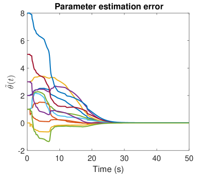
Figure 1: Trajectories of the parameter estimation errors using noise-free position measurements.

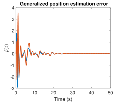
Figure 2: Trajectories of the generalized position estimation errors using noise-free position measurements.

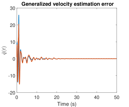
Figure 3: Trajectories of the generalized velocity estimation errors using noise-free position measurements.

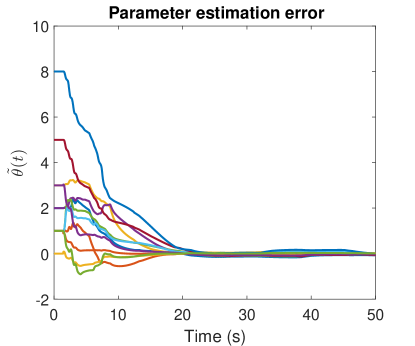
Figure 4: Trajectories of the parameter estimation errors with a Gaussian measurement noise (variance = 0.001).

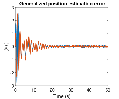
Figure 5: Trajectories of the generalized position estimation errors with a Gaussian measurement noise (variance = 0.001).

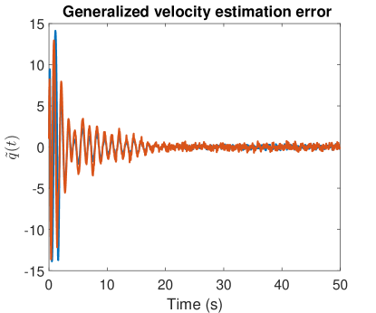
Figure 6: Trajectories of the generalized velocity estimation errors with a Gaussian measurement noise (variance = 0.001).

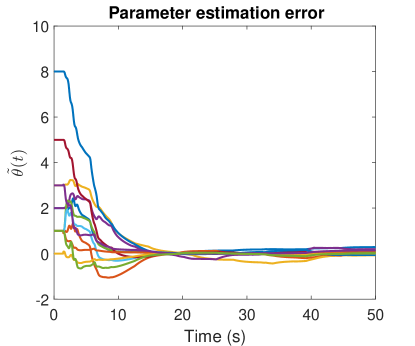
Figure 7: Trajectories of the parameter estimation errors with a Gaussian measurement noise (variance = 0.01).

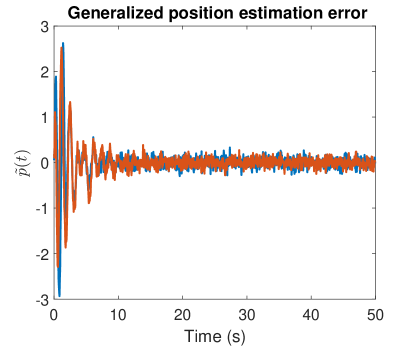
Figure 8: Trajectories of the generalized position estimation errors with a Gaussian measurement noise (variance = 0.01).

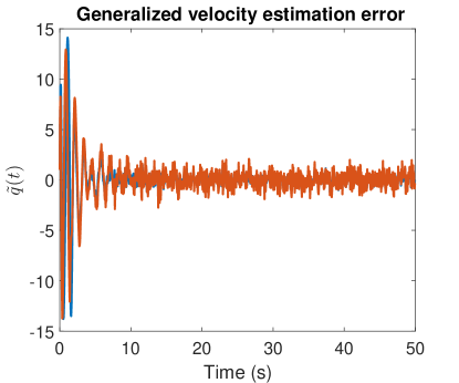
Figure 9: Trajectories of the generalized velocity estimation errors with a Gaussian measurement noise (variance = 0.01).

The linear system selected for the simulation study is given by

$$\dot{p}\left(t\right) =q\left(t\right),$$

$$\dot{q}\left(t\right) =\begin{bmatrix}2&3&1&5\\ 1&2&1&8\end{bmatrix}\begin{bmatrix}p\left(t\right)\\ q\left(t\right)\end{bmatrix}+\begin{bmatrix}1&3\\ 0&1\end{bmatrix}u\left(t\right),$$

The contribution of this paper is the design of a parameter estimator and a velocity observer. The controller is assumed to be any controller that results in bounded system response. In this simulation study, the controller, $u$, is designed so that the system tracks the trajectory $p_{1}\left(t\right)=p_{2}\left(t\right)=\sum_{j=1}^{3}\sin\left(jt\right)+\sin\left(5t\right)$. Since there are twelve unknown parameters and the desired trajectory contains only four distinct frequencies, the closed-loop system is not persistently excited.

The state observer in (16) is implemented using the integral form in (17), and the filter in (19) is implemented using the integral form in (21). The simulation is performed using Euler forward numerical integration using a sample time of $T_{s}=0.0005$ seconds. Past $\frac{T_{1}+T_{2}}{T_{s}}$ values of the generalized position, $p$, and the control input, $u$, are stored in a buffer. The matrices $\mathcal{F}$ and $\mathcal{G}$ for the parameter update law in (13) are computed using trapezoidal integration of the data stored in the aforementioned buffer. Values of $\mathcal{F}$ and $\mathcal{G}$ are stored in the history stack and are updated so as to maximize the minimum eigenvalue of $\mathscr{G}$.

The initial estimates of the unknown parameters are selected to be zero, and the history stack is initialized so that all the elements of the history stack are zero. Data is added to the history stack using a singular value maximization algorithm. To demonstrate the utility of the developed method, three simulation runs are performed. In the first run, the observer is assumed to have access to noise free measurements of the generalized position. In the second and the third runs, a zero-mean Gaussian noise with variance 0.001 and 0.01, respectively, is added to the generalized position signal to simulate measurement noise. The values of various simulation parameters selected for the three runs are available in Table I. Figure 1 demonstrates that in absence of noise, the developed parameter estimator drives the parameter estimation error, $\tilde{\theta}$, to the origin. Figures 2 and 3 demonstrates that the developed observer drives the generalized position and the generalized velocity estimation error to the origin, respectively. Figures 4 - 9 indicate that the developed method is applicable in the presence of measurement noise, with expected degradation of performance with increasing variance of the noise.

VII Conclusion

This paper develops a CL-based adaptive observer and parameter estimator to estimate the unknown parameter and the generalized velocity of second-order linear systems using generalized position measurements. The developed technique utilizes the fact that when integrated twice, the system dynamics can be reformulated as a set of algebraic equations that are linear in the unknown parameters. By integrating $n-$times, the developed method can be generalized to higher-order linear systems.

Simulation results indicate that the developed method is robust to measurement noise. A theoretical analysis of the developed method under measurement noise and process noise is a subject for future research. Future efforts will also focus on the examination the effect of the integration intervals, $T_{1}$ and $T_{2}$, on the performance of the observer.

References

- [1] P. Ioannou and J. Sun, Robust Adaptive Control. Prentice Hall, 1996.
- [2] S. Sastry and M. Bodson, Adaptive Control: Stability, Convergence, and Robustness. Upper Saddle River, NJ: Prentice-Hall, 1989.
- [3] M. Krstic, I. Kanellakopoulos, and P. V. Kokotovic, Nonlinear and Adaptive Control Design. New York, NY, USA: John Wiley & Sons, 1995.
- [4] M. A. Duarte and K. Narendra, “Combined direct and indirect approach to adaptive control,” IEEE Trans. Autom. Control, vol. 34, no. 10, pp. 1071–1075, Oct 1989.
- [5] M. Krstić, P. V. Kokotović, and I. Kanellakopoulos, “Transient-performance improvement with a new class of adaptive controllers,” Syst. Control Lett., vol. 21, no. 6, pp. 451 – 461, 1993.
- [6] G. V. Chowdhary and E. N. Johnson, “Theory and flight-test validation of a concurrent-learning adaptive controller,” J. Guid. Control Dynam., vol. 34, no. 2, pp. 592–607, Mar. 2011.
- [7] K. S. Narendra and A. M. Annaswamy, “A new adaptive law for robust adaptive control without persistent excitation,” IEEE Trans. Autom. Control, vol. 32, pp. 134–145, 1987.
- [8] K. Narendra and A. Annaswamy, “Robust adaptive control in the presence of bounded disturbances,” IEEE Trans. Autom. Control, vol. 31, no. 4, pp. 306–315, 1986.
- [9] K. Volyanskyy, A. Calise, B.-J. Yang, and E. Lavretsky, “An error minimization method in adaptive control,” in Proc. AIAA Guid. Navig. Control Conf., 2006.
- [10] G. Chowdhary, T. Yucelen, M. Mühlegg, and E. N. Johnson, “Concurrent learning adaptive control of linear systems with exponentially convergent bounds,” Int. J. Adapt. Control Signal Process., vol. 27, no. 4, pp. 280–301, 2013.
- [11] S. Kersting and M. Buss, “Concurrent learning adaptive identification of piecewise affine systems,” in IEEE Conf. Decis. Control, Dec. 2014, pp. 3930–3935.
- [12] G. Chowdhary, M. Mühlegg, J. How, and F. Holzapfel, “Concurrent learning adaptive model predictive control,” in Advances in Aerospace Guidance, Navigation and Control, Q. Chu, B. Mulder, D. Choukroun, E.-J. van Kampen, C. de Visser, and G. Looye, Eds. Springer Berlin Heidelberg, 2013, pp. 29–47.
- [13] H. Modares, F. L. Lewis, and M.-B. Naghibi-Sistani, “Integral reinforcement learning and experience replay for adaptive optimal control of partially-unknown constrained-input continuous-time systems,” Automatica, vol. 50, no. 1, pp. 193–202, 2014.
- [14] R. Kamalapurkar, J. Klotz, and W. E. Dixon, “Concurrent learning-based online approximate feedback Nash equilibrium solution of -player nonzero-sum differential games,” IEEE/CAA Journal of Automatica Sinica, Special Issue on Extensions of Reinforcement Learning and Adaptive Control, vol. 1, no. 3, pp. 239–247, Jul. 2014.
- [15] B. Luo, H.-N. Wu, T. Huang, and D. Liu, “Data-based approximate policy iteration for affine nonlinear continuous-time optimal control design,” Automatica, 2014.
- [16] R. Kamalapurkar, P. Walters, and W. E. Dixon, “Model-based reinforcement learning for approximate optimal regulation,” Automatica, vol. 64, pp. 94–104, Feb. 2016.
- [17] T. Bian and Z.-P. Jiang, “Value iteration and adaptive dynamic programming for data-driven adaptive optimal control design,” Automatica, vol. 71, pp. 348–360, 2016.
- [18] R. Kamalapurkar, J. A. Rosenfeld, and W. E. Dixon, “Efficient model-based reinforcement learning for approximate online optimal control,” Automatica, 2016, to appear.
- [19] G. D. L. Torre, G. Chowdhary, and E. N. Johnson, “Concurrent learning adaptive control for linear switched systems,” in Proc. Am. Control Conf., 2013, pp. 854–859.
- [20] G. Chowdhary, H. A. Kingravi, J. P. How, and P. A. Vela, “Bayesian nonparametric adaptive control using gaussian processes,” IEEE Trans. Neural Netw. Learn. Syst., vol. 26, no. 3, pp. 537–550, 2015.
- [21] R. Kamalapurkar, B. Reish, G. Chowdhary, and W. E. Dixon. Concurrent learning for parameter estimation using dynamic state-derivative estimators. arXiv:1507.08903.
- [22] A. Parikh, R. Kamalapurkar, and W. E. Dixon. Integral concurrent learning: Adaptive control with parameter convergence without PE or state derivatives. arXiv:1512.03464.
- [23] G. Chowdhary and E. Johnson, “Concurrent learning for convergence in adaptive control without persistency of excitation,” in IEEE Conf. Decis. Control, 2010, pp. 3674–3679.
- [24] B. Xian, M. S. de Queiroz, D. M. Dawson, and M. McIntyre, “A discontinuous output feedback controller and velocity observer for nonlinear mechanical systems,” Automatica, vol. 40, no. 4, pp. 695–700, 2004.
- [25] H. K. Khalil, Nonlinear Systems, 3rd ed. Upper Saddle River, NJ: Prentice Hall, 2002.