Analysis and optimization of weighted ensemble sampling

Abstract

We give a mathematical framework for weighted ensemble (WE) sampling, a binning and resampling technique for efficiently computing probabilities in molecular dynamics. We prove that WE sampling is unbiased in a very general setting that includes adaptive binning. We show that when WE is used for stationary calculations in tandem with a coarse model, the coarse model can be used to optimize the allocation of replicas in the bins.

65C05, 65C20, 65C40, 65Y05, 82C80

1 Introduction

This article concerns a resampling procedure, called weighted ensemble (WE), for Markov chains. WE consists of simulating some replicas of a Markov chain $(X_{p})_{p\geq 0}$ and resampling from the replicas at certain time intervals. In the literature, WE sampling [5, 8, 18, 23, 24, 29] usually refers to a resampling technique designed so that the replicas of $(X_{p})_{p\geq 0}$ are evenly distributed throughout state space. This is usually achieved by dividing state space into bins and resampling in each bin so that the number of replicas therein remains roughly constant. The replicas carry probabilistic weights so that the resulting statistical distribution is unbiased. This distribution can be used, in principle, to estimate any function of $(X_{p})_{p\geq 0}$ at a fixed time [29]. In practice, the quality of such estimates depends on the choice of bins and number of replicas maintained in each bin, among other factors. Below, we will usually refer to a replica as a particle and to resampling as selection, following convention in the mathematical literature.

Since WE is simply a resampling technique, it can be understood in a framework similar to that of particle filters or sequential Monte Carlo (SMC). For a review of standard SMC methods, see for instance the textbook [10], the articles [11, 12] or the compilation [13]. (See also [6, 7] for a related method.) We emphasize that WE does not fall into the SMC framework of [10], as there are no underlying potential functions or Gibbs-Boltzmann measures defining the selection step. We consider a very general framework for WE in which, contrary to the SMC/Feynman-Kac formalism (see [10]), the rule for killing or splitting replicas is essentially arbitrary. This means that WE requires an independent analysis.

The main contributions of this article are as follows. First, we give a definition of WE sampling that is bin-free and generalizes descriptions currently in the literature (Section 2). We prove WE is unbiased in this setting, which allows for adaptive selection procedures [29] (Section 3). Then, we give simple formulas for the variance of WE and show how, in principle, the variance can be minimized under a constraint on the number of particles (Sections 3-4). In practice, the variance formula contains terms that may not be efficiently computable. However, we show how a coarse model can be used to guide WE sampling to minimize variance in computations of fixed time as well as stationary averages of $(X_{p})_{p\geq 0}$ (Sections 5-8).

Our interest in WE arises from longstanding problems in computational chemistry. In this setting, $(X_{p})_{p\geq 0}$ is obtained from a discretization of some stochastic molecular dynamics (MD). MD simulations have proven useful for understanding many chemical and biological processes; see [22] for an overview. However, such simulations are limited by time scale separation. Many phenomena of interest occur at the laboratory time scale of microseconds, while MD simulations have time steps that correspond to femtoseconds. In this case, straightforward MD simulations are not practical. Many methods exist for extending the time scale of MD simulations; we do not attempt to give a review of them here. WE is one of several methods for extending the time scale of simulations in models with rough energy landscapes. Methods that are related in scope and design include Exact Milestoning [4, 15], Non-Equilibrium Umbrella Sampling [28, 25], Trajectory Tilting [26], Transition Interface Sampling [27], Forward Flux Sampling [1], and Boxed Molecular Dynamics [16]. See for instance [2, 9] for review and comparison of these methods. We will comment on Exact Milestoning in the Appendix below.

While WE can be used with a broad range of stochastic processes, when the process is time homogenous and Markovian – as in many models of MD, such as Langevin dynamics – WE may be used to efficiently compute dynamical quantities like reaction rates using a long time or stationary average [5, 24]. These computations rely on Hill’s relation [17], which we generalize in the Appendix below. From Hill’s relation, obtaining reaction rates requires a calculation using the stationary distribution of a nonreversible process.

To speed up the stationary calculation, WE is combined with a preconditioning step [5, 8] in which a Markov state model (MSM) [20, 21] is used to approximate the stationary distribution. This is sometimes called accelerated WE [8]. Accelerated WE begins with particles evenly distributed in space, with weights chosen to match the stationary distribution of the MSM. The particles are then allowed to relax according to their exact dynamics, with WE sampling ensuring that the particles remain evenly distributed in state space. We show below that information from the MSM can be used to optimize the WE sampling in this relaxation step, in the sense that the variance in the appropriate stationary calculation is minimized. This optimization requires an adaptive number of particles per bin, in contrast with traditional WE sampling. We show in a simple model that this adaptive sampling can be significantly better than traditional WE sampling.

This article is organized as follows. In Section 2, we define a WE process in a general setting and give an algorithm for WE sampling. In Section 3, we introduce a martingale framework for WE sampling in this setting. We use the framework to prove the sampling is unbiased and obtain formulas for the variance. In Section 4, we show how to minimize the variance under a constraint on the total number of particles. In Section 5 we consider WE sampling based on binning techniques. In Section 6 we show how adapting the binning to a coarse model for $(X_{p})_{p\geq 0}$ can be used to minimize variance, and in Section 7 we apply these ideas to computing stationary averages. In Section 8, we use a simple model to compare adaptive WE to traditional WE and naive sampling. In the Appendix, we prove a generalization of the Hill relation and discuss connections to Exact Milestoning.

2 Notation and assumptions

Throughout, $(X_{p})_{p\geq 0}$ is a time homogeneous Markov chain with values in a measurable space $(E,{\mathcal{E}})$ and transition kernel $K$. We write $\sim$ to denote equality in law of random variables or processes, and ${\mathbb{E}}$ and ${\mathbb{P}}$ for various expectations and probabilities. When $\zeta$ is a probability measure on $(E,{\mathcal{E}})$, superscripts such as ${\mathbb{E}}^{\zeta}$ or ${\mathbb{P}}^{\zeta}$ represent processes with initial distribution $\zeta$, with ${\mathbb{E}}^{x}$ or ${\mathbb{P}}^{x}$ indicating the processes start at the point $x$. Sets and functions will be assumed measurable without explicit mention. For a measure $\zeta$ on $(E,{\mathcal{E}})$ and bounded $f:E\to{\mathbb{R}}$, we write $\zeta(f)=\int f\,d\zeta$ for the integral of $f$ with respect to $\zeta$. We also write $\zeta K(dy)=\int K(x,dy)\zeta(dx)$ for left action of $K$, and $Kf(x)=\int K(x,dy)f(y)$ for the right action. In particular,

(1) $$\zeta K^{n}f={\mathbb{E}}^{\zeta}[f(X_{n})]$$

where throughout $K$ is the Markov transition kernel of $(X_{p})_{p\geq 0}$. If $S$ is a set, we write $\#S$ for the number of elements of $S$.

We study a certain class of sequential Monte Carlo (SMC) methods for sampling $(X_{p})_{p\geq 0}$ described in Definition 2.1 below. We begin with an informal description of the procedure. Consider a process consisting of particles in $E$ and weights in ${\mathbb{R}}^{+}=[0,\infty)$. The initial particles all have the same distribution as $X_{0}$. At each time $p$, some of the particles are selected, or copied, and others are thrown away, or killed. The selected particles then mutate according to the evolution law of $(X_{p})_{p\geq 0}$. (We often refer to selected particles as children and the particles from which they were copied as parents.) The selected points and weights are chosen to yield unbiased estimators for the law of $(X_{p})_{p\geq 0}$. This is ensured by setting a child’s weight to be its parent’s weight divided by the expected number of times the parent is selected. Writing $\xi_{p}^{j}$ and $\omega_{p}^{j}$ for the particles and weights at time $p$, and using the symbol “$\,\,\hat{}\,\,$” to indicate selected particles and weights, we make this precise as follows.

Definition 2.1.

A weighted ensemble (WE) consists of particles and weights

$$(\xi_{p}^{j},\omega_{p}^{j})_{p\geq 0}^{j=1,\ldots,N_{p}},\qquad({\hat{\xi}}_{p}^{i},{\hat{\omega}}_{p}^{i})_{p\geq 0}^{i=1,\ldots,{\hat{N}}_{p}}$$

with values in $\cup_{n=1}^{\infty}(E\times{\mathbb{R}}^{+})^{n}$, selection rules

$$(C_{p}^{j})_{p\geq 0}^{j=1,\ldots,N_{p}}$$

with values in $\cup_{n=1}^{\infty}({\mathbb{N}}\cup\{0\})^{n}$, and associated filtrations

$${\mathcal{F}}_{p} =\sigma\left((\xi_{q}^{j},\omega_{q}^{j})_{0\leq q\leq p}^{j=1,\ldots,N_{q}},(C_{q}^{j})_{0\leq q\leq p-1}^{j=1,\ldots,N_{q}},({\hat{\xi}}_{q}^{i},{\hat{\omega}}_{q}^{i})_{0\leq q\leq p-1}^{i=1,\ldots,{\hat{N}}_{q}}\right)$$

$${\hat{\mathcal{F}}}_{p} =\sigma\left((\xi_{q}^{j},\omega_{q}^{j})_{0\leq q\leq p}^{j=1,\ldots,N_{q}},(C_{q}^{j})_{0\leq q\leq p}^{j=1,\ldots,N_{q}},({\hat{\xi}}_{q}^{i},{\hat{\omega}}_{q}^{i})_{0\leq q\leq p}^{i=1,\ldots,{\hat{N}}_{q}}\right)$$

which together satisfy (A1)-(A4) below for each $p\geq 0$.

• $N_{0}>0$ is constant, and for $j=1,\ldots,N_{0}$, $\xi_{0}^{j}\sim X_{0}$, $\omega_{0}^{j}=1/N_{0}$.

• Each child ${\hat{\xi}}_{p}^{i}$ is associated to a parent $\xi_{p}^{\alpha(i)}$. With

  $$C_{p}^{j}=\#\{i:\alpha(i)=j\}$$

  the number of children of $\xi_{p}^{j}$, we have ${\mathbb{E}}[C_{p}^{j}|{\mathcal{F}}_{p}]>0$,

  $${\hat{N}}_{p}=\sum_{j=1}^{N_{p}}C_{p}^{j},\qquad\text{and}\qquad{\hat{\omega}}_{p}^{i}=\frac{\omega_{p}^{j}}{{\mathbb{E}}\left[C_{p}^{j}|{\mathcal{F}}_{p}\right]},\quad\text{ if }\alpha(i)=j.$$

• Conditionally on ${\mathcal{F}}_{p}$, $C_{p}^{1},\ldots,C_{p}^{N_{p}}$ are uncorrelated.

• $N_{p+1}={\hat{N}}_{p}$ and $\omega_{p+1}^{i}={\hat{\omega}}_{p}^{i}$ for $i=1,\ldots,{\hat{N}}_{p}$.

• Conditionally on ${\hat{\mathcal{F}}}_{p}$, $\xi_{p+1}^{1},\ldots,\xi_{p+1}^{N_{p+1}}$ are independent with

  $${\mathbb{P}}[\xi_{p+1}^{i}\in dx]=K({\hat{\xi}}_{p}^{i},dx).$$

It is convenient to view a WE through the following diagram:

$$\{\xi_{p}^{j}\}^{j=1,\ldots,N_{p}}\xrightarrow{\textup{selection}}\{{\hat{\xi}}_{p}^{i}\}^{i=1,\ldots,{\hat{N}}_{p}}\xrightarrow{\textup{mutation}}\{{\xi}_{p+1}^{j}\}^{j=1,\ldots,N_{p+1}},$$

$$\{\omega_{p}^{j}\}^{j=1,\ldots,N_{p}}\xrightarrow{\textup{selection}}\{{\hat{\omega}}_{p}^{i}\}^{i=1,\ldots,{\hat{N}}_{p}}\xrightarrow{\textup{mutation}}\{{\omega}_{p+1}^{j}\}^{j=1,\ldots,N_{p+1}}.$$

The filtration ${\mathcal{F}}_{p}$ (resp. ${\hat{\mathcal{F}}}_{p}$) represents the information from the WE process up to time $p$, not including the selection step (resp. up to time $p$, including the selection step). We write $\alpha(i)$ for the index of the parent particle of the $i$th selected particle. Thus,

$$\alpha(i)=j\Longrightarrow{\hat{\xi}}_{p}^{i}=\xi_{p}^{j}.$$

(Of course $\alpha$ depends on $p$, but we do not make this explicit.) Also,

$$C_{p}^{j}=\#\{i:\alpha(i)=j\}=\text{number of times }\xi_{p}^{j}\text{ is selected}.$$

The $C_{p}^{j}$, $j=1,\ldots,N_{p}$, can depend on the entire history of the process. We assume in (A2’) that they are uncorrelated conditionally on the past so that we can obtain a relatively simple explicit formula for variance in Theorem 3.1 below. This assumption is only needed for the variance. Indeed, the proof of Theorem 3.1 below shows that (A2’) is not required for unbiased WE sampling; see the remarks after the proof of Theorem 3.1.

Note that, by (A2), the weight of a selected particle is simply the weight of its parent particle divided by the expected number of times the parent is selected. We assume the expected number of times a parent is selected is positive, so that each particle has a positive probability to survive.

Assumption (A1) says that the initial collection of particles and weights is chosen according to the distribution of $X_{0}$. Notice we do not require that the $\xi_{0}^{i}$’s are independent, so they can be generated by, for example, Markov chain Monte Carlo or other sequential samplers.

Algorithm 1 A WE sampler

Choose initial points and weights $(\xi_{0}^{j},\omega_{0}^{j})^{j=1,\ldots,N_{0}}$ according to the distribution of $X_{0}$ in the sense of (A1). Then iterate over $p\geq 0$ until time $\tau_{kill}:=\inf\{p\geq 0:N_{p}=0\}$:

• For $j=1,\ldots,N_{p}$, choose a number $C_{p}^{j}$ of times to select particle $\xi_{p}^{j}$. Let ${\hat{\xi}}_{p}^{i}$, $i=1,\ldots,{\hat{N}}_{p}$ be the collection of selected particles, with ${\hat{N}}_{p}=\sum_{j=1}^{N_{p}}C_{p}^{j}$.

• Assign the weight ${\hat{\omega}}_{p}^{i}=\frac{\omega_{p}^{j}}{{\mathbb{E}}[C_{p}^{j}|{\mathcal{F}}_{p}]}$ to ${\hat{\xi}}_{p}^{i}$, if $\alpha(i)=j$.

• Set $N_{p+1}={\hat{N}}_{p}$ and $\omega_{p+1}={\hat{\omega}}_{p}^{i}$ for $i=1,\ldots,{\hat{N}}_{p}$.

• Evolve the particles ${\hat{\xi}}_{p}^{i}$, $i=1,\ldots,{\hat{N}}_{p}$, independently according to the law of $(X_{p})_{p\geq 0}$ to get the next generation $\xi_{p+1}^{j}$, $j=1,\ldots,N_{p+1}$ of particles.

Steps 1-2 correspond to selection, and 3-4 to evolution. In the above, the $C_{p}^{j}$’s are usually independent of each other, given the current state of the algorithm, and they can depend on the entire history of the algorithm up to time $p$. In Step 2, ${\mathbb{E}}[C_{p}^{j}|{\mathcal{F}}_{p}]$ represents the expected value of $C_{p}^{j}$ given that history. We assume ${\mathbb{E}}[C_{p}^{j}|{\mathcal{F}}_{p}]>0$, that is, every particle has a positive survival probability.

Assumption (A3) says that the weights defined in the selection step will be assigned to the particles in the next generation. The condition (A4) states that the next generation of particles mutates from the selected particles using the evolution law of $(X_{p})_{p\geq 0}$, where these particles evolve independently from each other.

For clarity, we give an algorithm for sampling a WE process; see Algorithm 1.

We will show in Theorem 3.1 below that a WE in the sense of Definition 2.1 is an unbiased estimator for the law of $(X_{p})_{p\geq 0}$. To make this precise we introduce the following notation. At time $p$, a WE defines empirical distributions

(2) $$\eta_{p}=\sum_{j=1}^{N_{p}}\omega_{p}^{j}\delta_{\xi_{p}^{j}},\qquad{\hat{\eta}}_{p}=\sum_{i=1}^{{\hat{N}}_{p}}{\hat{\omega}}_{p}^{i}{\delta}_{{\hat{\xi}}_{p}^{i}}.$$

These definitions make sense only up until the first time all the particles have been killed, $\tau_{kill}=\inf\{p\geq 0:{N}_{p}=0\}=\inf\{p\geq 0:{\hat{N}}_{p-1}=0\}$. We adopt the convention that $\eta_{p}\equiv 0$ and ${\hat{\eta}}_{p-1}\equiv 0$ if $p\geq\tau_{kill}$. It is important to note that $\eta_{p}(1)\neq 1$ in general; that is, the total weight is not conserved exactly.

Remark 2.2.

Often it is desirable to fix the average total number of particles, or simply the total number of particles. Below we consider mostly the former case, but here we comment briefly on the latter.

A simple population control step can be added to guarantee $N_{p}\equiv N$ for each $p$, with $N$ fixed, as follows. First, assume the population control has been applied up to time $p$, so that $N_{p}=N$. Suppose furthermore that the selection is done so that ${\mathbb{E}}[N_{p+1}|\mathcal{F}_{p}]=N$. Then

$$N={\mathbb{E}}[{\hat{N}}_{p}|\mathcal{F}_{p}]={\mathbb{E}}\left[\left.\sum_{j=1}^{N_{p}}C_{p}^{j}\right|\mathcal{F}_{p}\right]=\sum_{j=1}^{N}{\mathbb{E}}[C_{p}^{j}|{\mathcal{F}}_{p}].$$

It follows that ${\mathbb{E}}[C_{p}^{j}|{\mathcal{F}}_{p}]\geq 1$ for some $j$. For this $j$ we may assume $C_{p}^{j}\geq 1$ with probability $1$, conditional on ${\mathcal{F}}_{p}$. Thus, we can assume there is no extinction in the selection step. Then, after the selection step, we can kill or copy particles uniformly at random to enforce $N_{p+1}=N$, and adjust weights accordingly. Note that this extra step would introduce correlations between the number of children of each particle, which would violate (A2’). So that we can obtain simple variance formulas, below we will focus on the case of uncorrelated $C_{p}^{j}$’s.

3 Martingale framework and variance

Recall that $K$ is the transition kernel of $(X_{p})_{p\geq 0}$, and recall the definitions of $\eta_{p}$ and ${\hat{\eta}}_{p}$ from (2). In this section and below, $n\geq 0$ and a bounded function $f:E\to{\mathbb{R}}$ are fixed. For $0\leq p\leq n$ define

$$M_{p}=\eta_{p}K^{n-p}f,\qquad{\hat{M}}_{p}={\hat{\eta}}_{p}K^{n-p}f,$$

where by convention $K^{0}f=f$. Since $f$ is bounded, both $(M_{p})_{0\leq p\leq n}$ and $({\hat{M}}_{p})_{0\leq p\leq n}$ are integrable and square integrable. Intuitively, $M_{p}$ represents starting at the distribution $\eta_{p}$, evolving forward $n-p$ time steps using $K$, and then evaluating $f$; see (1). Our analysis below is based on the following result.

Theorem 3.1.

Let assumptions (A1), (A2), (A3), and (A4) hold. Then $(M_{p})_{0\leq p\leq n}$ is a ${\mathcal{F}}_{p}$-martingale and

(3) $${\mathbb{E}}[M_{n}^{2}]={\mathbb{E}}[M_{0}^{2}]+{\mathbb{E}}\left[\sum_{p=0}^{n-1}\left({\mathbb{E}}\left[(M_{p+1}-{\hat{M}}_{p})^{2}|\hat{\mathcal{F}}_{p}\right]\right]+{\mathbb{E}}\left[({\hat{M}}_{p}-M_{p})^{2}|{\mathcal{F}}_{p}\right]\right).$$

If in addition (A2’) holds, then with $g_{p}=K^{n-p}f$,

(4) $$\begin{split}&{\mathbb{E}}\left[\left.(M_{p+1}-{\hat{M}}_{p})^{2}\right|{\hat{\mathcal{F}}}_{p}\right]=\sum_{i=1}^{{\hat{N}}_{p}}({\hat{\omega}}_{p}^{i})^{2}[Kg_{p+1}^{2}({\hat{\xi}}_{p}^{i})-g_{p}({\hat{\xi}}_{p}^{i})^{2}]\\ &{\mathbb{E}}\left[\left.({\hat{M}}_{p}-M_{p})^{2}\right|{\mathcal{F}}_{p}\right]=\sum_{j=1}^{N_{p}}({\omega}_{p}^{j})^{2}\left[\frac{{\mathbb{E}}[(C_{p}^{j})^{2}|{\mathcal{F}}_{p}]}{{\mathbb{E}}[C_{p}^{j}|{\mathcal{F}}_{p}]^{2}}-1\right]g_{p}(\xi_{p}^{j})^{2}\end{split}$$

for $0\leq p\leq n-1$.

Proof 3.2.

Consider a WE as in Definition 2.1. From (A4),

(5) $${\mathbb{E}}\left[\left.g_{p+1}(\xi_{p+1}^{i})\right|\hat{{\mathcal{F}}_{p}}\right]=Kg_{p+1}({\hat{\xi}}_{p}^{i})=g_{p}({\hat{\xi}}_{p}^{i}).$$

If in addition (A2’) holds, then

(6) $${\mathbb{E}}\left[\left.g_{p+1}(\xi_{p+1}^{i})g_{p+1}(\xi_{p+1}^{k})\right|\hat{{\mathcal{F}}_{p}}\right]=\begin{cases}g_{p}({\hat{\xi}}_{p}^{i})g_{p}({\hat{\xi}}_{p}^{k}),&i\neq k\\ Kg_{p+1}^{2}({\hat{\xi}}_{p}^{i}),&i=k\end{cases}.$$

Suppose (A1), (A2), (A3) and (A4) hold. We show that then

$$M_{0},{\hat{M}}_{0},M_{1},{\hat{M}}_{1},\ldots,{\hat{M}}_{n-1},M_{n}$$

is a martingale with respect to the filtration

$${\mathcal{F}}_{0}\subseteq\hat{\mathcal{F}}_{0}\subseteq{\mathcal{F}}_{1}\subseteq\hat{\mathcal{F}}_{1}\subseteq\ldots\subseteq\hat{\mathcal{F}}_{n-1}\subseteq{\mathcal{F}}_{n}.$$

That is, we show that for $0\leq p\leq n-1$,

$${\mathbb{E}}[M_{p+1}|\hat{\mathcal{F}}_{p}]=\hat{M}_{p},\qquad{\mathbb{E}}[{\hat{M}}_{p}|{\mathcal{F}}_{p}]=M_{p}.$$

The fact that $M_{p}$ is a martingale then follows from

$${\mathbb{E}}[M_{p+1}|{\mathcal{F}}_{p}]={\mathbb{E}}[{\mathbb{E}}[M_{p+1}|\hat{\mathcal{F}}_{p}]|{\mathcal{F}}_{p}]={\mathbb{E}}[{\hat{M}}_{p}|{\mathcal{F}}_{p}]=M_{p},$$

and equation (3) follows from the Doob decomposition. Since $g_{p}=K^{n-p}f$,

$$M_{p}=\sum_{j=1}^{N_{p}}\omega_{p}^{j}g_{p}(\xi_{p}^{j}),\qquad{\hat{M}}_{p}=\sum_{i=1}^{{\hat{N}}_{p}}{\hat{\omega}}_{p}^{i}g_{p}({\hat{\xi}}_{p}^{i}).$$

So by (A3) and (5),

$${\mathbb{E}}[M_{p+1}|\hat{\mathcal{F}}_{p}] ={\mathbb{E}}\left[\left.\sum_{i=1}^{N_{p+1}}\omega_{p+1}^{i}g_{p+1}(\xi_{p+1}^{i})\right|\hat{\mathcal{F}}_{p}\right]$$

$$=\sum_{i=1}^{{\hat{N}}_{p}}{\hat{\omega}}_{p}^{i}{\mathbb{E}}[g_{p+1}(\xi_{p+1})|\hat{\mathcal{F}}_{p}]$$

$$=\sum_{i=1}^{{\hat{N}}_{p}}{\hat{\omega}}_{p}^{i}g_{p}({\hat{\xi}}_{p}^{i})={\hat{M}}_{p}.$$

Also, by (A2),

$${\mathbb{E}}[{\hat{M}}_{p}|{\mathcal{F}}_{p}] ={\mathbb{E}}\left[\left.\sum_{i=1}^{{\hat{N}}_{p}}{\hat{\omega}}_{p}^{i}g_{p}({\hat{\xi}}_{p}^{i})\right|{\mathcal{F}}_{p}\right]$$

$$=\sum_{j=1}^{N_{p}}{\mathbb{E}}\left[\left.\sum_{i:\alpha(i)=j}{\hat{\omega}}_{p}^{i}g_{p}({\hat{\xi}}_{p}^{i})\right|{\mathcal{F}}_{p}\right]$$

$$=\sum_{j=1}^{N_{p}}\frac{\omega_{p}^{j}}{{\mathbb{E}}[C_{p}^{j}|{\mathcal{F}}_{p}]}{\mathbb{E}}\left[\left.\sum_{i:\alpha(i)=j}g_{p}({\hat{\xi}}_{p}^{i})\right|{\mathcal{F}}_{p}\right]$$

$$=\sum_{j=1}^{N_{p}}\omega_{p}^{j}g_{p}(\xi_{p}^{j})=M_{p}.$$

It remains to establish (LABEL:eq_l2explicit). Suppose in addition (A2’) holds. By (6) and (A3),

$${\mathbb{E}}[M_{p+1}^{2}|\hat{\mathcal{F}}_{p}] ={\mathbb{E}}\left[\left.\sum_{i,k=1}^{N_{p+1}}\omega_{p+1}^{i}\omega_{p+1}^{k}g_{p+1}(\xi_{p+1}^{i})g_{p+1}(\xi_{p+1}^{k})\right|\hat{\mathcal{F}}_{p}\right]$$

$$=\sum_{i,k=1}^{{\hat{N}}_{p}}{\hat{\omega}}_{p}^{i}{\hat{\omega}}_{p}^{k}{\mathbb{E}}\left[\left.g_{p+1}(\xi_{p+1}^{i})g_{p+1}(\xi_{p+1}^{k})\right|\hat{\mathcal{F}}_{p}\right]$$

$$=\sum_{\begin{subarray}{c}i,k=1\\ i\neq k\end{subarray}}^{{\hat{N}}_{p}}{\hat{\omega}}_{p}^{i}{\hat{\omega}}_{p}^{k}g_{p}({\hat{\xi}}_{p}^{i})g_{p}({\hat{\xi}}_{p}^{k})+\sum_{i=1}^{{\hat{N}}_{p}}({\hat{\omega}}_{p}^{i})^{2}Kg_{p+1}^{2}({\hat{\xi}}_{p}^{i}).$$

Subtracting ${\hat{M}}_{p}^{2}$ from this gives

$${\mathbb{E}}[(M_{p+1}-{\hat{M}}_{p})^{2}|\hat{\mathcal{F}}_{p}]={\mathbb{E}}[M_{p+1}^{2}|\hat{\mathcal{F}}_{p}]-{\hat{M}}_{p}^{2}=\sum_{i=1}^{{\hat{N}}_{p}}({\hat{\omega}}_{p}^{i})^{2}[Kg_{p+1}^{2}({\hat{\xi}}_{p}^{i})-g_{p}({\hat{\xi}}_{p}^{i})^{2}].$$

Next, notice that, with $\beta_{p}^{j}={\mathbb{E}}[C_{p}^{j}|{\mathcal{F}}_{p}]$, by (A2),

$${\mathbb{E}}[{\hat{M}}_{p}^{2}|{\mathcal{F}}_{p}] ={\mathbb{E}}\left[\left.\sum_{i,k=1}^{{\hat{N}}_{p}}{\hat{\omega}}_{p}^{i}{\hat{\omega}}_{p}^{k}g_{p}({\hat{\xi}}_{p}^{i})g_{p}({\hat{\xi}}_{p}^{k})\right|{\mathcal{F}}_{p}\right]$$

$$=\sum_{j,\ell=1}^{N_{p}}\frac{\omega_{p}^{j}\omega_{p}^{\ell}}{\beta_{p}^{j}\beta_{p}^{\ell}}{\mathbb{E}}\left[\left.\sum_{i,k:\alpha(i)=j,\alpha(k)=\ell}g_{p}({\hat{\xi}}_{p}^{i})g_{p}({\hat{\xi}}_{p}^{k})\right|{\mathcal{F}}_{p}\right],$$

Summing over $j\neq\ell$ and using (A2’), we get

$$\sum_{\begin{subarray}{c}j,\ell=1\\ j\neq\ell\end{subarray}}^{N_{p}}\frac{\omega_{p}^{j}\omega_{p}^{\ell}}{\beta_{p}^{j}\beta_{p}^{\ell}}{\mathbb{E}}\left[\left.\sum_{i,k:\alpha(i)=j,\alpha(k)=\ell}g_{p}({\hat{\xi}}_{p}^{i})g_{p}({\hat{\xi}}_{p}^{k})\right|{\mathcal{F}}_{p}\right]=\sum_{\begin{subarray}{c}j,\ell=1\\ j\neq\ell\end{subarray}}^{N_{p}}\omega_{p}^{j}\omega_{p}^{\ell}g_{p}(\xi_{p}^{j})g_{p}(\xi_{p}^{\ell}),$$

and summing over $j=\ell$, with $\gamma_{p}^{j}={\mathbb{E}}[(C_{p}^{j})^{2}|{\mathcal{F}}_{p}]$, we have

$$\sum_{j=1}^{N_{p}}\left(\frac{\omega_{p}^{j}}{\beta_{p}^{j}}\right)^{2}{\mathbb{E}}\left[\left.\sum_{i,k:\alpha(i)=j,\alpha(k)=j}g_{p}({\hat{\xi}}_{p}^{i})g_{p}({\hat{\xi}}_{p}^{k})\right|{\mathcal{F}}_{p}\right]=\sum_{j=1}^{N_{p}}\left(\frac{\omega_{p}^{j}}{\beta_{p}^{j}}\right)^{2}\gamma_{p}^{j}g_{p}(\xi_{p}^{j})^{2}.$$

Combining the last three displays,

$${\mathbb{E}}[{\hat{M}}_{p}^{2}|{\mathcal{F}}_{p}]=\sum_{\begin{subarray}{c}j,\ell=1\\ j\neq\ell\end{subarray}}^{N_{p}}\omega_{p}^{j}\omega_{p}^{\ell}g_{p}(\xi_{p}^{j})g_{p}(\xi_{p}^{\ell})+\sum_{j=1}^{N_{p}}\left(\frac{\omega_{p}^{j}}{\beta_{p}^{j}}\right)^{2}\gamma_{p}^{j}g_{p}(\xi_{p}^{j})^{2}.$$

Subtracting $M_{p}^{2}$, we get

$${\mathbb{E}}[({\hat{M}}_{p}-M_{p})^{2}|{\mathcal{F}}_{p}]={\mathbb{E}}[{\hat{M}}_{p}^{2}|{\mathcal{F}}_{p}]-M_{p}^{2}=\sum_{j=1}^{N_{p}}\left[\left(\frac{\omega_{p}^{j}}{\beta_{p}^{j}}\right)^{2}\gamma_{p}^{j}-(\omega_{p}^{j})^{2}\right]g_{p}(\xi_{p}^{j})^{2}.$$

Below, we will repeatedly refer to the functions

$$g_{p}=K^{n-p}f$$

from the proof above, so we record the definition here again for convenience. We note that Theorem 3.1 shows WE is unbiased, as follows. Since $(M_{p})_{0\leq p\leq n}$ is a martingale, ${\mathbb{E}}[M_{n}]={\mathbb{E}}[M_{0}]$. Moreover, (A1) implies ${\mathbb{E}}[M_{0}]={\mathbb{E}}[f(X_{n})]$. This means that

$${\mathbb{E}}\left[\sum_{j=1}^{N_{n}}\omega_{n}^{j}f(\xi_{n}^{j})\right]={\mathbb{E}}\left[M_{n}\right]={\mathbb{E}}[f(X_{n})].$$

The proof of Theorem 3.1 shows that this equation does not require assumption (A2’). Notice also that (3) leads to a formula for the $L^{2}$ sampling error, or variance, via

(7) $$\begin{split}{\mathbb{E}}\left[\left(\sum_{j=1}^{N_{n}}\omega_{n}^{j}f(\xi_{n}^{j})-{\mathbb{E}}[f(X_{n})]\right)^{2}\right]&={\mathbb{E}}\left[(M_{n}-{\mathbb{E}}[f(X_{n})])^{2}\right]\\ &={\mathbb{E}}[M_{n}^{2}]-{\mathbb{E}}[f(X_{n})]^{2}.\end{split}$$

By Theorem 3.1, the expression in (7) consists of a term corresponding to the variance from the initial condition, namely ${\mathbb{E}}[M_{0}^{2}]-{\mathbb{E}}[f(X_{n})]^{2}=\text{Var}(M_{0})$, added to another term corresponding to the variance from the evolutions and selections, namely

$${\mathbb{E}}\left[\sum_{p=0}^{n-1}\left({\mathbb{E}}\left[(M_{p+1}-{\hat{M}}_{p})^{2}|\hat{\mathcal{F}}_{p}\right]\right]+{\mathbb{E}}\left[({\hat{M}}_{p}-M_{p})^{2}|{\mathcal{F}}_{p}\right]\right).$$

If we assume (A2’), we can get nice expressions for the latter variances; see (LABEL:eq_l2explicit). In (LABEL:eq_l2explicit), we can think of the first equation as the variance due to mutation, and the second equation as the variance from selection. Indeed we can understand these as “local variances” associated to particle evolution and selection since we can rewrite

$${\mathbb{E}}\left[\left.(M_{p+1}-{\hat{M}}_{p})^{2}\right|{\hat{\mathcal{F}}}_{p}\right]=\sum_{i=1}^{{\hat{N}}_{p}}({\hat{\omega}}_{p}^{i})^{2}\text{Var}_{K({\hat{\xi}}_{p}^{i},\cdot)}(g_{p+1})$$

and

$${\mathbb{E}}\left[\left.({\hat{M}}_{p}-M_{p})^{2}\right|{\mathcal{F}}_{p}\right]=\sum_{j=1}^{N_{p}}({\omega}_{p}^{j})^{2}\frac{\textup{Var}(C_{p}^{j}|{\mathcal{F}}_{p})}{{\mathbb{E}}[C_{p}^{j}|{\mathcal{F}}_{p}]^{2}}g_{p}(\xi_{p}^{j})^{2}.$$

In the following sections we will attempt to minimize these terms to produce a near optimal sampling strategy.

4 Minimizing variance

The main idea in the sections that follow is to use information available at time $p$ – that is, the ${\mathcal{F}}_{p}$-measurable random variables – to decide how to make the selections. We want to minimize the variance from both selection and mutation, subject to a constraint on the average total number of particles. Instead of trying to simultaneously minimize both variances, we will minimize in two steps: first, we minimize the variance from mutation, and then, subject to the constraints thereby imposed, we minimize the variance from selection.

For the variance from mutation, we have to condition on ${\mathcal{F}}_{p}$ to get an expression that depends only on ${\mathcal{F}}_{p}$-measurable random variables. Thus, using (LABEL:eq_l2explicit) and (A2),

(8) $$\begin{split}{\mathbb{E}}\left[\left.(M_{p+1}-{\hat{M}}_{p})^{2}\right|{\mathcal{F}}_{p}\right]&={\mathbb{E}}\left[\left.{\mathbb{E}}\left[\left.(M_{p+1}-{\hat{M}}_{p})^{2}\right|\hat{\mathcal{F}}_{p}\right]\right|{\mathcal{F}}_{p}\right]\\ &={\mathbb{E}}\left[\left.\sum_{i=1}^{{\hat{N}}_{p}}({\hat{\omega}}_{p}^{i})^{2}[Kg_{p+1}^{2}({\hat{\xi}}_{p}^{i})-g_{p}({\hat{\xi}}_{p}^{i})^{2}]\right|{\mathcal{F}}_{p}\right]\\ &=\sum_{j=1}^{N_{p}}\left(\frac{\omega_{p}^{j}}{{\mathbb{E}}[C_{p}^{j}|{\mathcal{F}}_{p}]}\right)^{2}{\mathbb{E}}\left[\left.\sum_{i:\alpha(i)=j}[Kg_{p+1}^{2}({\hat{\xi}}_{p}^{i})-g_{p}({\hat{\xi}}_{p}^{i})^{2}]\right|{\mathcal{F}}_{p}\right]\\ &=\sum_{j=1}^{N_{p}}\frac{(\omega_{p}^{j})^{2}}{{\mathbb{E}}[C_{p}^{j}|{\mathcal{F}}_{p}]}[Kg_{p+1}^{2}(\xi_{p}^{j})-g_{p}(\xi_{p}^{j})^{2}].\end{split}$$

Minimizing this expression is only interesting if we limit the total number of particles. In principle, we can choose $C_{p}^{j}$’s such that this variance is minimized, given a fixed target number, $N$, of total particles. More precisely, if we demand that

$$\sum_{j=1}^{N_{p}}{\mathbb{E}}[C_{p}^{j}|{\mathcal{F}}_{p}]=N,$$

then a Lagrange multiplier calculation shows (8) is minimized by $C_{p}^{j}$’s with

(9) $${\mathbb{E}}[C_{p}^{j}|{\mathcal{F}}_{p}]=\frac{N\omega_{p}^{j}\sqrt{Kg_{p+1}^{2}(\xi_{p}^{j})-g_{p}(\xi_{p}^{j})^{2}}}{\sum_{j=1}^{N_{p}}\omega_{p}^{j}\sqrt{Kg_{p+1}^{2}(\xi_{p}^{j})-g_{p}(\xi_{p}^{j})^{2}}}.$$

(provided the denominator above is nonzero). Note that from Jensen’s inequality,

$$Kg_{p+1}^{2}(\xi)-g_{p}(\xi)^{2}=\text{Var}_{K(\xi,\cdot)}(g_{p+1})\geq 0$$

for all $\xi\in E$, and indeed this expression can be understood as a “local variance” associated with mutating a particle $\xi$. Recall the variance due to selection is

(10) $${\mathbb{E}}\left[\left.({\hat{M}}_{p}-M_{p})^{2}\right|{\mathcal{F}}_{p}\right]=\sum_{j=1}^{N_{p}}(\omega_{p}^{j})^{2}\left[\frac{{\mathbb{E}}[(C_{p}^{j})^{2}|{\mathcal{F}}_{p}]}{{\mathbb{E}}[C_{p}^{j}|{\mathcal{F}}_{p}]^{2}}-1\right]g_{p}(\xi_{p}^{j})^{2}.$$

Our minimization strategy is as follows. First, we choose $C_{p}^{j}$’s satisfying (9). Note that this step only determines their average values

$$\beta_{p}^{j}={\mathbb{E}}[C_{p}^{j}|{\mathcal{F}}_{p}].$$

To minimize (10) over these $C_{p}^{j}$’s, we take ${\mathbb{E}}[(C_{p}^{j})^{2}|{\mathcal{F}}_{p}]$ as small as possible. This is done as follows. Let $\lfloor x\rfloor$ be the integer part of $x$. Then conditionally on ${\mathcal{F}}_{p}$, set each $C_{p}^{j}$ to equal either $\lfloor\beta_{p}^{j}\rfloor$ or $\lfloor\beta_{p}^{j}\rfloor+1$, with probabilities chosen so that the mean is $\beta_{p}^{j}$.

The problem with the above strategy is that, in (9), the quantities

$$Kg_{p+1}^{2}(\xi_{p}^{j})-g_{p}(\xi_{p}^{j})^{2}$$

are not easily computable. Indeed, if they were, then $(X_{p})_{p\geq 0}$ would be simple enough that WE is not needed. We have found that nonetheless a version of the above strategy can be made useful if we obtain coarse approximations for these quantities. The basic idea is to construct a coarse model, for instance a Markov State Model [20, 21], for $(X_{p})_{p\geq 0}$ from which the $Kg_{p+1}^{2}(\xi_{p}^{j})-g_{p}(\xi_{p}^{j})^{2}$ can be approximated. The coarse model will have states that correspond to bins that partition $E$, and the WE process will be adapted to the same bins, in the sense that the resampling rules are tailored to the bin structure. We pursue these ideas in the following sections.

Remark 4.1.

It is interesting to consider the limits where the time or the number of particles become infinite. We briefly comment on the latter. If we substitute the minimizing equation (9) into (8), and set

$$F(\xi):=\sqrt{Kg_{p+1}^{2}(\xi)-g_{p}(\xi)^{2}},$$

then we get

(11) $$N{\mathbb{E}}\left[\left.(M_{p+1}-{\hat{M}}_{p})^{2}\right|{\mathcal{F}}_{p}\right]=\left(\sum_{j=1}^{N_{p}}\omega_{p}^{j}F(\xi_{p}^{j})\right)^{2}=(\eta_{p}(F))^{2}.$$

Intuitively, under appropriate conditions on $F$, the following particle approximation result is suggested by a version of the law of large numbers for sufficiently weakly dependent random variables:

$$\eta_{p}(F)\xrightarrow{a.s.}{\mathbb{E}}[F(X_{p})]\quad\text{ as }N\to\infty.$$

We leave this question for future work; see however Section 7.4 of [10] for analogous results in the SMC/Feyman-Kac framework. Taking this result for granted and using (11), we expect ${\mathbb{E}}[F(X_{p})]^{2}$ to be the normalized asymptotic variance from mutation for the strategy described above. We compare this to naive simulation ($C_{p}^{j}\equiv 1$ for all $p$ and $j$ and $N_{p}\equiv N$ for all $p$) where by the law of large numbers,

$$N{\mathbb{E}}\left[\left.(M_{p+1}-{\hat{M}}_{p})^{2}\right|{\mathcal{F}}_{p}\right]=\frac{1}{N}\sum_{j=1}^{N}F(\xi_{p}^{j})^{2}\xrightarrow{a.s.}{\mathbb{E}}[F(X_{p})^{2}]\quad\text{ as }N\to\infty,$$

so that ${\mathbb{E}}[F(X_{p})^{2}]$ is the normalized asymptotic variance from mutation.

5 Binning

In traditional WE, the number of times $C_{p}^{j}$ we select particle $\xi_{p}^{j}$ is based on a binning technique. At each time step $p$, state space $E$ is divided into disjoint bins $B^{r}$, $r=1,\ldots,R$. That is, $E=\cup_{r=1}^{R}B^{r}$ where the union is disjoint. In general, the bins can be chosen adaptively; see Remark 5.1. However, we will focus on fixed bins here and below. In this setting, the selection step proceeds as follows. First, a target number of particles $N_{p}^{r}$ is set for each bin at time $p$. In many applications (see for instance [5, 23, 24, 29] and references), the target numbers are chosen so that the resulting particles cover space uniformly in some sense, which usually means $N_{p}^{r}\approx N/R$. We will take a different approach in the next section. The $C_{p}^{j}$’s are chosen such that either

(12) $$\sum_{j:\xi_{p}^{j}\in B^{r}}{\mathbb{E}}[C_{p}^{j}|{\mathcal{F}}_{p}]=N_{p}^{r},$$

or, conditionally on ${\mathcal{F}}_{p}$,

(13) $$\sum_{j:\xi_{p}^{j}\in B^{r}}C_{p}^{j}=N_{p}^{r}.$$

In the latter case (13), the number of particles in a given bin has a fixed deterministic value, while in the former (12), only the average number of particles in each bin is fixed. See Remark 2.2 above. In (12), as discussed above, the $C_{p}^{j}$’s are usually chosen to have small variance, so the number of particles in a given bin has small variance. Throughout we will focus only on the case (12). Note that number of selected particles in bin $B^{r}$, namely

$$\sum_{j:\xi_{p}^{j}\in B^{r}}C_{p}^{j},$$

can equal zero. However, under assumption (A2), whenever there are particles in $B^{r}$ at time $p$, the expected number $N_{p}^{r}$ of selected particles in $B^{r}$ must be strictly positive. It is okay if there are no particles in a bin before selection – that bin will just remain empty after the selection step.

Remark 5.1.

We will use bins that are fixed in time. This stance allows us, in principle at least, to define a Markov state model [20, 21] on the bins. This model can, in turn, be useful for minimizing the variance in (3). We note, however, that the bins can be chosen adaptively and still fit the framework of Definition 2.1. For example, the bins can be deterministic functions of the particles and weights up to and including the current time. Theorem 3.1 then demonstrates that WE samping is unbiased even when the bins are adaptively chosen.

Algorithm 2 Constructing a coarse model

Choose bins $B^{1},\ldots,B^{R}$ forming a partition of $E$, a sampling measure $\zeta$ on $(E,{\mathcal{E}})$, and a bounded function $f:E\to{\mathbb{R}}$. Then do the following.

• Estimate the probability ${P}_{rs}$ for $(X_{p})_{p\geq 0}$ to go from $B^{r}$ to $B^{s}$ in one step:

  $$P_{rs}=\zeta(B^{r})^{-1}\int_{B^{r}}{\mathbb{P}}\left[\left.X_{p+1}\in B^{s}\right|X_{p}=x\right]\,\zeta(dx).$$

  Estimate the value of $f$ inside bin $B^{r}$ by $u_{r}$:

  $$u_{r}=\zeta(B^{r})^{-1}\int_{B^{r}}f(x)\,\zeta(dx).$$

• Let $v_{p}^{r}$ be the $r$th entry of the vector $P(P^{n-p-1}u)^{2}-(P^{n-p}u)^{2}$, where $u=(u_{r})$ is considered a column vector and the squaring operations are entrywise.

• Let $\mu$ be the stationary distribution for the transition matrix $P=(P_{rs})$. That is, ${\mu}=(\mu_{r})$ is the normalized left eigenvector of $P$ with eigenvalue $1$.

$P$ and $u$ in Step 1 can be obtained sampling many one-step trajectories starting at $\zeta$. A simple choice for $\zeta$ in a general setting would be the uniform (Lebesgue) measure. See also the Appendix for comments on another possibility for $\zeta$.

6 Adapting to a coarse model

Suppose we have a coarse model for $(X_{p})_{p\geq 0}$ and we want to use it to guide our sampling. As above, we fix $n\geq 0$ and a bounded function $f:E\to{\mathbb{R}}$. The coarse model will be adapted to some fixed choice of bins; we assume again that $E$ is divided into disjoint bins $B^{r}$, $r=1,\ldots,R$. We think of the coarse model as a Markov state model, where the states are the bins. More precisely, the coarse model will consist of approximations of the probability $P_{rs}$ that $X_{p+1}\in B^{s}$, given that $X_{p}\in B^{r}$, as well as estimates $u_{r}$ of the value of $f$ on $B^{r}$. Thinking of $P$ as a matrix and $u$ a column vector, let

$$v_{p}^{r}=r\text{th entry of the vector }P(P^{n-p-1}u)^{2}-(P^{n-p}u)^{2},$$

where the squaring operations are entrywise. Then $v_{p}^{r}$ estimates the value in $B^{r}$ of

$$Kg_{p+1}^{2}-g_{p}^{2}\equiv K(K^{n-p-1}f)^{2}-(K^{n-p}f)^{2}.$$

Below we show how to use the coarse model to define a WE sampler so that $\eta_{n}(f)$ estimates ${\mathbb{E}}[f(X_{n})]$ with small variance, using an approximate version of the strategy described in Section 4. Because we are using a coarse model that does not distinguish between points in a given bin, it is reasonable to take all the selected weights ${\hat{\omega}}_{p}^{i}$ of particles in a given bin $B^{r}$ to have the same value ${\bar{\omega}}_{p}^{r}$:

(14) $${\hat{\omega}}_{p}^{i}={\bar{\omega}}_{p}^{r},\qquad\text{if }{\hat{\xi}}_{p}^{i}\in B^{r}.$$

This type of weighting scheme is simply a choice of the practitioner. In particular, it leads to a class of WE samplers satisfying Definition 2.1, as follows. In light of Definition 2.1, the number of times $\xi_{p}^{j}\in B^{r}$ is selected is

(15) $${\mathbb{E}}[C_{p}^{j}|{\mathcal{F}}_{p}]=\frac{\omega_{p}^{j}}{{\bar{\omega}}_{p}^{r}},\qquad\text{if }\xi_{p}^{j}\in B^{r}.$$

Setting the average number of particles in $B^{r}$ as $N_{p}^{r}$ as in (12), we obtain

(16) $${\bar{\omega}}_{p}^{r}=\frac{\sum_{j:\xi_{p}^{j}\in B^{r}}\omega_{p}^{j}}{N_{p}^{r}}.$$

Thus, the weighting scheme in (14), together with a choice of target particle numbers $N_{p}^{r}$, leads to unique formulas for the selected weights and the expected number of children of each particle.

From (9), the variance from mutation is minimized when

(17) $$\begin{split}N_{p}^{r}&\equiv\sum_{j:\xi_{p}^{j}\in B^{r}}{\mathbb{E}}[C_{p}^{j}|{\mathcal{F}}_{p}]\\ &=\sum_{j:\xi_{p}^{j}\in B^{r}}\frac{N\omega_{p}^{j}\sqrt{Kg_{p+1}^{2}(\xi_{p}^{j})-g_{p}(\xi_{p}^{j})^{2}}}{\sum_{\ell=1}^{N_{p}}\omega_{p}^{\ell}\sqrt{Kg_{p+1}^{2}(\xi_{p}^{\ell})-g_{p}(\xi_{p}^{\ell})^{2}}}\\ &\approx\frac{N\sqrt{v_{p}^{r}}\sum_{j:\xi_{p}^{j}\in B^{r}}\omega_{p}^{j}}{\sum_{r=1}^{R}\sqrt{v_{p}^{r}}\sum_{j:\xi_{p}^{j}\in B^{r}}\omega_{p}^{j}}.\end{split}$$

In Algorithms 3- 4, the $C_{p}^{j}$’s are independent with

(18) $$C_{p}^{j}=\begin{cases}\lfloor\omega_{p}^{j}/{\bar{\omega}}_{p}^{r}\rfloor,&\text{w.p.}\quad 1-\left(\omega_{p}^{j}/{\bar{\omega}}_{p}^{r}-\lfloor\omega_{p}^{j}/{\bar{\omega}}_{p}^{r}\rfloor\right)\\ \lfloor\omega_{p}^{j}/{\bar{\omega}}_{p}^{r}\rfloor+1,&\text{w.p.}\quad\omega_{p}^{j}/{\bar{\omega}}_{p}^{r}-\lfloor\omega_{p}^{j}/{\bar{\omega}}_{p}^{r}\rfloor\end{cases},\qquad\text{if }\xi_{p}^{j}\in B^{r},$$

where $\lfloor x\rfloor$ denotes the integer part of $x$, and the $N_{p}^{r}$’s are defined by

(19) $$N_{p}^{r}:=\frac{(N-{\tilde{N}}R)\sqrt{v_{p}^{r}}\sum_{i:\xi_{p}^{i}\in B^{r}}\omega_{p}^{i}}{\sum_{r=1}^{R}\sqrt{v_{p}^{r}}\sum_{i:\xi_{p}^{i}\in B^{r}}\omega_{p}^{i}}+{\tilde{N}},$$

where ${\tilde{N}}\in(0,N/R)$ is a lower threshold for the target number of particles per bin, and by convention $N_{p}^{r}={\tilde{N}}$ if the denominator in (19) is zero. The $C_{p}^{j}$’s in (18) have been chosen to minimize the variance due to selection over all possible choices satisfying (15). See Algorithms 3 and 4 for implementations of these ideas.

Algorithm 3 A WE sampler adapted to a coarse model

Choose bins $B_{r}$, $r=1,\ldots,R$ forming a partition of $E$, a target total number of particles $N$, a lower threshold ${\tilde{N}}$, a final time $n$, and a bounded function $f:E\to{\mathbb{R}}$. Let $v_{p}^{r}$ be obtained as in Algorithm 2. Choose initial points and weights with the distribution of $X_{0}$ in the sense of (A1). For $0\leq p\leq\min\{n,\tau_{kill}\}$, iterate the following:

• Select $N_{p}^{r}$ according to (19) and define ${\bar{\omega}}_{p}^{r}$ as in (16).

• Let $C_{p}^{j}$ be random variables defined by (18), and select $\xi_{p}^{j}$ exactly $C_{p}^{j}$ times. Let ${\hat{\xi}}_{p}^{i}$, $i=1,\ldots,{\hat{N}}_{p}$ be the selected particles, with ${\hat{N}}_{p}=\sum_{j=1}^{N_{p}}C_{p}^{j}$.

• Set $N_{p+1}={\hat{N}}_{p}$ and assign the weight ${\omega}_{p+1}^{i}={\bar{\omega}}_{p}^{r}$ if ${\hat{\xi}}_{p}^{i}\in B^{r}$.

• Evolve the particles ${\hat{\xi}}_{p}^{i}$, $i=1,\ldots,{\hat{N}}_{p}$, independently according to the law of $(X_{p})_{p\geq 0}$ to get the next generation $\xi_{p+1}^{i}$, $i=1,\ldots,N_{p+1}$ of particles.

When $p=\min\{n,\tau_{kill}\}$, stop and output $\eta_{n}(f)$, an estimate of ${\mathbb{E}}[f(X_{n})]$.

Why did we set a lower threshold ${\tilde{N}}$ in (19)? If ${\tilde{N}}=0$ and $v_{p}^{r}$ is zero in a bin that contains particles, then no particles can be selected in this bin and so (A2) does not hold. Taking ${\tilde{N}}>0$ eliminates this problem by ensuring $N_{p}^{r}>0$ in each bin so that each particle has a positive survival probability.

Moreover, if $v_{p}^{r}$ is very small in some bins and large in others, if ${\tilde{N}}=0$ then some selected particles can have very large weights due to a tiny value of $N_{p}^{r}$ in (16). While this is fine in principle – the method is still unbiased – we observed numerically that it is better to keep a target number of particles per bin that is bounded significantly away from zero. Note that, as desired, the expected number of selected particles is

$$\sum_{r=1}^{R}N_{p}^{r}=N,$$

unless $v_{p}^{r}=0$ in every bin that contains particles, in which case we instead have

$$\sum_{r=1}^{R}N_{p}^{r}={\tilde{N}}R.$$

If $\sum_{r=1}^{R}N_{p}^{r}<N_{p}$, then it is possible that ${\mathbb{E}}[C_{p}^{j}|{\mathcal{F}}_{p}]<1$ for all $j$. If in addition the $C_{p}^{j}$’s are independent conditional on ${\mathcal{F}}_{p}$, then there is a strictly positive probability that all particles are killed in selection, that is, $\tau_{kill}=p+1$. However, we believe extinction is a remote possibility with an appropriate choice of parameters. Indeed in our simulations we did not observe any events where all the particles were killed so long as $N$ was kept reasonably large and ${\tilde{N}}$ not too close to zero; see Section 8 below.

7 Stationary averages

In this section, let $(X_{p})_{p\geq 0}$ have a unique stationary distribution $\pi$. Suppose we want to sample $\pi(f)$, where $f:E\to{\mathbb{R}}$ is bounded. Assume we have bins $B^{r}$, $r=1,\ldots,R$, and a coarse model for $(X_{p})_{p\geq 0}$ as in the last section. This model consists of a coarse transition matrix $P$ which can be used to estimate variances as discussed above. Note that $P$ can also be used to estimate $\pi$. That is, the stationary vector $\mu$ of $P$ – namely, the normalized left eigenvector for eigenvalue $1$ – is a coarse estimate of $\pi$.

To sample $\pi(f)$, we can begin with points approximately distributed according to $\pi$ in the some sense. Using the coarse model, and beginning with $N$ points roughly uniformly distributed in space, we take initial points and weights with

(20) $$\#\{j:\xi_{0}^{j}\in B^{r}\}\approx\frac{N}{R},\qquad\omega_{0}^{j}=\frac{\mu_{r}}{\#\{k:\xi_{0}^{k}\in B^{r}\}},\quad\text{if }\xi_{0}^{j}\in B^{r}.$$

The final time $n$ should be large enough to allow the WE sampler to relax to the true stationary distribution $\pi$. Techniques which employ a coarse model to estimate $\pi$, and use this as an initial condition for WE, have appeared recently in [5, 8]. However, using the coarse model to minimize the variance in the above fashion appears to be new, to the best of our knowledge. In this context, minimizing the variance requires minimal additional work, since we already have the coarse transition matrix $P$ which can be used to estimate the quantities needed to minimize variance.

The question of how to choose the final time $n$ is difficult in general. Note, however, that we have some prior information from our coarse model. In particular, the second-largest (in absolute value) eigenvalue $\lambda_{2}$ of $P$ can give us some idea of how fast convergence can be, from the heuristic

$${\mathbb{E}}[\eta_{n}(f)]-\pi(f)\approx O(\lambda_{2}^{n}).$$

Moreover the constant associated with the big O may be small due to the initial condition (20), though this is difficult to quantify without prior information about how close the initial condition is to $\pi$.

Remark 7.1.

We comment briefly on two other possibilities for sampling $\pi(f)$.

First, we could build the coarse model adaptively, using a Monte Carlo estimator of $v_{p}^{r}$. That is, we update $v_{p}^{r}$ at each time $p$ using the WE trajectory. One advantage of this is that, if we are using $\eta_{n}(f)$ to estimate $\pi(f)$, the most important contributions to the variance come from the final steps ($p$ near $n$), at which $v_{p}^{r}$ is the most accurate.

Another possibility is, instead of estimating $\pi(f)$ from $\eta_{n}(f)$, we could use a time average via $\pi(f)\approx(n+1)^{-1}(\eta_{0}(f)+\ldots+\eta_{n}(f))$. In this setting, it is natural to adaptively build estimates $v^{r}$ of $Kf^{2}-(Kf)^{2}$ in $B^{r}$, and plug them into (19) in place of the $v_{p}^{r}$ at each step. We do not test these strategies here, but leave them as interesting problems for future work.

8 Numerical example

In this section $(Y_{t})_{t\geq 0}$ is an Markov chain designed to mimic MD in a simple one dimensional energy landscape, and $X_{p}=Y_{p\delta t}$. In the context of WE, this means we resample from $(Y_{t})_{t\geq 0}$ at each time interval $\delta t$. Our goal is to show that the adaptive sampling from the last section potentially can be better than naive sampling or traditional WE sampling. Applying these ideas to more “realistic” models in computational chemistry will be the focus of another work.

Algorithm 4 A WE sampler for stationary averages

Choose bins $B_{r}$, $r=1,\ldots,R$, a target total number of particles $N$, a final time $n$, and a bounded function $f:E\to{\mathbb{R}}$. Construct a coarse model as in Algorithm 2.

• Choose initial points and weights as in (20).

• For $0\leq p\leq\min\{n,\tau_{kill}\}$, proceed through Algorithm 3.

The output $\eta_{n}(f)$ is an estimate of $\pi(f)$, the stationary average of $f$.

More precisely, let $Y_{t}$ have values in $E=\{1,2,\ldots,90\}$ and transition matrix

$$Q(i,i+1) =\frac{2}{5}+\frac{m(i)}{5},\qquad i=1,\ldots,89,$$

$$Q(i,i-1) =\frac{2}{5}-\frac{m(i)}{5},\qquad i=2,\ldots,90,$$

where

$$m(j):=\sin\left(\frac{6\pi j}{90}\right),$$

$Q(i,j)=0$ if $|i-j|>1$ and $Q(i,i)$ is chosen so that $Q$ is stochastic. This is a discrete state space which mimics a one dimensional potential energy landscape with $3$ energy wells; see the bottom right of Figure 2. We take resampling intervals $\delta t=4$, so

$$X_{p}:=Y_{4p}$$

and the transition matrix of $(X_{p})_{p\geq 0}$ is $K=Q^{4}$. The resampling intervals are chosen so that a sufficiently large fraction of particles can change bins in each resampling time. The bins will be

$$B^{r}=\{3r-2,3r-1,3r\},\qquad r=1,\ldots,30.$$

Thus, there are $R=30$ bins. Let $\pi$ be the stationary distribution of $(X_{p})_{p\geq 0}$, and

$$f(i)=\begin{cases}1,&28\leq i\leq 33\\ 0,&\text{else}\end{cases}.$$

We also let ${\bar{f}}=f/6$ be its normalized version, which is useful for comparing with sampling distributions; see Figure 2 below.

We will obtain empirical approximations $\eta_{n}(f)$ of $\pi(f)$ for relaxation times $n=5,10,15,20,25,30$, using three types of sampling described below. In all our simulations, we set a target number $N=150$ of particles, Our initial particles and weights are the same for all simulations. They are chosen by constructing a coarse model as in Algorithm 2 with $\zeta$ the uniform measure on $E$, $\zeta(i)=1/90$ for all $i\in E$. Thus, our initial points and weights are chosen according to the distribution

$$\nu_{0}(i)=\frac{\mu_{r}}{3},\qquad\text{if }i\in B^{r}.$$

In all our simulations we had $\tau_{kill}>n$.

The first type of sampling uses Algorithm 4, the procedure described above for adapting WE to a coarse model. We call this adaptive WE sampling. We construct a coarse model using Algorithm 2 with the uniform sampling measure $\zeta$ described above. We use the parameters $N=150$ and ${\tilde{N}}=1$.

In the second type of sampling we used a fixed target number of particles per bin. We call this traditional WE sampling. It is the sampling method described in [5, 8]. We use Algorithm 4 again, but instead of using a coarse model to define $N_{p}^{r}$ via (19), we set $N_{p}^{r}=5$ constant. This corresponds to distributing the $N=150$ particles uniformly among the bins.

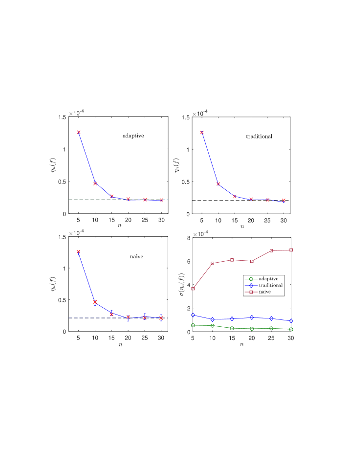
Figure 1: Values of $\eta_{n}(f)$ vs. $n$ from the example in Section 8 from adaptive, traditional and naive sampling. Data for adaptive, traditional and naive sampling is obtained from $10^{3}$, $10^{4}$, and $5\times 10^{4}$ independent simulations, respectively. The crosses are exact values corresponding to $\nu_{0}K^{n}f$, and the dotted line is the stationary value $\pi(f)$. Bottom right: sample standard deviations $\sigma(\eta_{n}(f))$ of $\eta_{n}(f)$, computed from the independent simulations. (The error bars in the other plots are these standard deviations divided by the square roots of the number of independent simulations.)

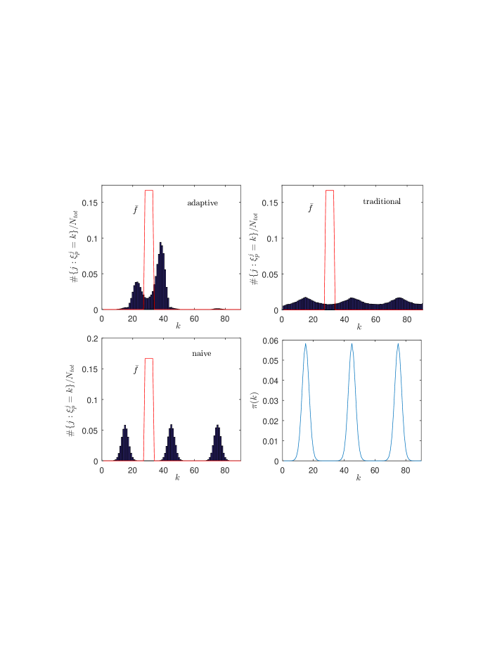
Figure 2: Average distribution of particles $\xi_{p}^{j}$ at time $n=30$, compared to ${\bar{f}}$, the normalized version of $f$. Here, $N_{tot}\equiv N_{n}$ is the total number of particles at time $n$. Bottom right: Stationary distribution $\pi$.

The third type of sampling does not use selection at all. We call this naive sampling. Here, we choose $N=150$ initial particles and weights according to (20), and then we simply evolve these particles independently until time $n$, without changing the weights.

Results comparing adaptive WE sampling, traditional WE sampling and naive sampling are in Figures 1-2. In Figure 1, we plot $\eta_{n}(f)$ vs. $n$ for various values of $n$, showing convergence to the stationary value $\pi(f)$. We compute error bars using empirical standard deviations from $10^{3}$, $10^{4}$ and $5\times 10^{4}$ independent simulations for adaptive, traditional, and naive sampling respectively. (We had to run more simulations for traditional WE and naive sampling to get the numerics to converge.) The sample standard deviation for adaptive WE sampling is significantly smaller than that of traditional WE and naive sampling.

In Figure 2, we plot histograms representing the average distribution of the particles $\xi_{n}^{i}$ at time $n$. Note that traditional WE sampling distributes the particles roughly uniformly in space, as expected, while adaptive WE sampling guides the particles towards the region in state space relevant for computing $f$. Meanwhile, naive sampling distributes the particles approximately according to the stationary distribution $\pi$.

In Figure 3, we plot the estimates $v_{p}^{r}$ from the adaptive sampling strategy for $p=0$ and $p=n-1$ where $n=30$ is the relaxation time. Note that by time $n-1$, the sampling is focused near the support of $f$.

When $f$ is a function with large values in regions of low $\pi$ probability, as in this example, naive sampling performs poorly compared to both traditional and adaptive WE sampling. When state space is very large compared to the region $S$ where $f$ has large values (or is non-negligible), we expect adaptive WE sampling to perform much better than traditional WE sampling, due to the fact that traditional WE sampling will distribute the particles very thinly throughout space, including in $S$, while adaptive WE sampling will push most of the particles towards $S$.

A possible drawback of adaptive WE sampling is that it requires more computations at the resampling times, compared to traditional WE sampling. However, in practice the resampling times may be large enough so that this extra effort contributes little to the overall computational cost.

Finally, we note that the adaptive sampling above can also be used more generally to estimate time marginals of $(X_{p})_{p\geq 0}$, that is, expectations of the form ${\mathbb{E}}[f(X_{n})]$ at fixed finite times $n$, from an arbitrary initial distribution of $X_{0}$. This is Algorithm 3. In this case, a MSM is still required to guide the sampling. One of the advantages of the adaptive sampling in the stationary case is that a MSM has already been computed as part of a preconditioning step.

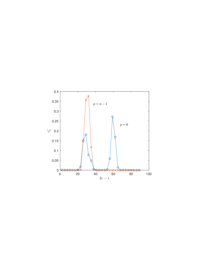
Figure 3: The estimates $v_{p}^{r}$ vs. $p$ for the example in Section 8. Here, we take $p=0$ and $p=n-1$, where $n=30$ is the final time.

Appendix: Computing dynamics from stationary averages

In this Appendix we show how to compute certain dynamical averages of $(X_{p})_{p\geq 0}$ from stationary calculations. As above, $(X_{p})_{p\geq 0}$ is a time homogeneous Markov chain with values in $E$. The Hill relation [17] shows that a mean hitting time can be reformulated as a certain stationary average. Similar ideas have recently been adapted to the time inhomogeneous setting; see [25]. Here we focus on the time homogeneous case.

By way of motivation, suppose we have a Markov chain with a (perhaps time reversible) transition kernel $K_{0}$. Suppose we are interested in averages of the Markov chain, starting at a distribution $\rho$ and up to the hitting time $\tau_{F}$ of some set $F$ disjoint from the support of $\rho$. To compute such averages, we consider a modified, non-time reversible transition kernel $K$ constructed by setting $K=K_{0}$ outside $F$ and $K=\rho K_{0}$ inside $F$. Clearly, if we can sample from $K_{0}$, then we can also sample from $K$, simply by sampling from $K_{0}$ outside $F$ and then instantaneously restarting at $\rho$ each time we reach $F$. The following result recasts an average of the Markov chain with kernel $K_{0}$ starting at $\rho$ and up to time $\tau_{F}$ as a stationary average of the nonreversible Markov chain with kernel $K$.

Theorem 8.1.

Suppose there is a set $F\subseteq E$ and a probability measure $\rho$ on $E$ with support disjoint from $F$ such that:

• The transition kernel $K$ of $(X_{p})_{p\geq 0}$ satisfies ${\mathbbm{1}}_{F}(x)K(x,dy)=\rho K(dy)$,

• With $\tau_{F}=\inf\{p>0\,:\,X_{p}\in F\}$, ${\mathbb{E}}^{\rho}[\tau_{F}]<\infty$ and ${\mathbb{P}}^{x}[\tau_{F}<\infty]=1$ $\forall x\in E$.

Then for any bounded $g:E\to{\mathbb{R}}$,

(21) $${\mathbb{E}}^{\rho}\left[\sum_{p=1}^{\tau_{F}}g(X_{p})\right]=\frac{\pi(g)}{\pi(F)},$$

where $\pi$ is the unique stationary distribution of $(X_{p})_{p\geq 0}$.

Proof 8.2.

Assumptions (B1)-(B2) show that $(X_{p})_{p\geq 0}$ has a unique stationary distribution $\pi$. Indeed, it can be checked (see [14], Section 5.6) that

$$\pi(A)=\dfrac{{\mathbb{E}}^{\rho}\left[\sum_{p=1}^{\tau_{F}}{\mathbbm{1}}_{A}(X_{p})\right]}{{\mathbb{E}}^{\rho}[\tau_{F}]}.$$

Thus,

$$\frac{\pi(g)}{\pi(F)}=\dfrac{{\mathbb{E}}^{\rho}\left[\sum_{p=1}^{\tau_{F}}g(X_{p})\right]}{{\mathbb{E}}^{\rho}\left[\sum_{p=1}^{\tau_{F}}\mathbbm{1}_{F}(X_{p})\right]}={\mathbb{E}}^{\rho}\left[\sum_{p=1}^{\tau_{F}}g(X_{p})\right].$$

In practice, we are interested in the left hand side of (21). Assumption (B1) can be understood as introducing a source $\rho$ and sink at $F$, while (B2) is an additional technical condition which ensures $\pi$ exists and is unique. In the context of the discussion above, (B1) corresponds to modifying the kernel $K_{0}$ of some underlying process to get the nonreversible kernel $K$. This modification is only a computational tool, as it does not affect the LHS of (21).

Thus, though the process we are interested in usually does not satisfy (B1), we can modify it in $F$ so that (B1) holds, and meanwhile the left hand side of (21) is the same for both the original and modified process. In this setting, if the original process is reversible, it is natural to take the sampling measure $\zeta$ in Algorithm 2 to be its stationary distribution, provided it can be efficiently calculated by Markov chain Monte Carlo or other common sampling techniques for reversible processes. It is important to note that such techniques cannot be used to directly sample $\pi$, since the modified process is nonreversible.

Two special cases of (21) are of particular interest. First, suppose $F=A\cup B$ is a disjoint union, $g={\mathbbm{1}}_{B}$, and $\tau_{S}=\inf\{p>0:X_{p}\in S\}$ is the first time to hit $S$. Then

(22) $${\mathbb{P}}^{\rho}\left[\tau_{B}<\tau_{A}\right]=\frac{\pi(B)}{\pi(A\cup B)}.$$

Next, suppose $g\equiv{\mathbbm{1}}$. Then

(23) $${\mathbb{E}}^{\rho}[\tau_{F}]=\frac{1}{\pi(F)}.$$

Equation (23) is known as the Hill relation [17]. Equations (22) and (23) show how stationary calculations can be used to compute hitting probabilities and hitting times. We can compute the right hand side of (22) by applying Algorithm 4 above to $f={\mathbbm{1}}_{B}$ and then $f={\mathbbm{1}}_{A\cup B}$. Similarly, we can compute the right hand side of (23) by applying Algorithm 4 with $f={\mathbbm{1}}_{F}$. A simple choice for $\rho$ would be $\rho=\delta_{x}$, the delta distribution at a point $x\notin F$. A more complicated but important case is the so-called equilibrium hitting time between an initial set $I$ and final set $F$; see for instance [3] for definitions and discussion. In this case, $\rho$ is the distribution of endpoints of trajectories under the original kernel $K_{0}$ stopped upon hitting $I$ and which last came from $F$. Sampling this distribution can be difficult in general [3].

We conclude by briefly connecting the discussion above to Exact Milestoning [2, 4], an algorithm mentioned in the Introduction for sampling dynamical quantities like mean hitting times. Consider the following seemingly more general framework. Suppose that $(Y_{t})_{t\geq 0}$ is some underlying process and $(\tau_{p})_{p\geq 0}$ are increasing stopping times for $(Y_{t})_{t\geq 0}$ such that $(X_{p})_{p\geq 1}$ defined by

$$X_{p}=(Y_{\tau_{p-1}+1},\ldots,Y_{\tau_{p}})$$

is a time homogeneous Markov chain in $\cup_{n=1}^{\infty}E^{n}$. For instance, if $(Y_{t})_{t\geq 0}$ is a time homogeneous Markov chain, we could take $\tau_{p}=p\delta t$ with $\delta t$ a deterministic time, as in the example in Section 8, or $\tau_{p}=\inf\{t>\tau_{p-1}:Y_{t}\in S\}$ for some set $S\subseteq E$, and $\tau_{0}=0$. The latter choice corresponds to Exact Milestoning, in which $S$ corresponds to the union of all the milestones. In this setting, if we take $g(X_{p})=\tau_{p}-\tau_{p-1}$, $F=\cup_{n=1}^{\infty}(E^{n-1}\times R)$, and

$$T_{R}=\inf\{\tau_{p}>0:Y_{\tau_{p}}\in R\},$$

then from (21),

(24) $${\mathbb{E}}^{\rho}[T_{R}]=\frac{{\mathbb{E}}^{\pi}[\tau_{1}]}{\pi(F)}.$$

This is the equation on which Exact Milestoning is based; see for instance Theorem 3.4 of [2]. Thus in Exact Milestoning, we can find the time $T_{R}$ for $Y_{t}$ to first reach $R$ starting at $\rho$ by computing $\pi(F)$ along with short trajectories of $Y_{t}$ starting at $\pi$ up to the first time to hit $S$.

References

- [1] R.J. Allen, D. Frenkel, and P.R. ten Wolde, Forward flux sampling-type schemes for simulating rare events: Efficiency analysis, J. Chem. Phys. 124(19), (2006), pp. 463102.
- [2] Aristoff, D., Bello-Rivas, J.M., and Elber, R., A mathematical framework for exact milestoning, Multiscale Model. Simul. 14(1), (2016), 301–322.
- [3] Bhatt, D. and Zuckerman, D., Beyond Microscopic Reversibility: Are Observable Nonequilibrium Processes Precisely Reversible?, J. Chem. Theory Comput. 7(8), (2011), 2520–2527.
- [4] Bello-Rivas, J. M. and Elber, R., Exact milestoning, The Journal of Chemical Physics, 142 (2015), pp. 094102.
- [5] Bhatt, D., Zhang, B.W., and Zuckerman, D.M. Steady-state simulations using weighted ensemble path sampling, J. Chem. Phys. 133, (2010), 014110.
- [6] Cérou, F. and Guyader, A. Adaptive Multilevel Splitting for Rare Event Analysis, Stoch. Anal. Appl. 25(2), (2007), 417–443.
- [7] Cérou, F. and Guyader, A., Lelièvre, T. and Pommier, D. A multiple replica approach to simulate reactive trajectories, J. Chem. Phys. 134, (2011), 054108.
- [8] Costaouec, R., Feng, H., Izaguirre, J., and Darve, E. Analysis of the accelerated weighted ensemble methodology, Supplement, Discrete and Continuous Dynamical Systems, 2013.
- [9] Darve, E. and Ryu, E. Computing reaction rates in bio-molecular systems using discrete macro-states, Innovations in Biomolecular Modeling and Simulations, RSC publishing, 2012.
- [10] Del Moral, P. Feynman-Kac Formulae: Genealogical and Interacting Particle Systems with Applications, Probability and Its Applications, Springer, 2004.
- [11] Del Moral, P. and Doucet, A. Particle methods: an introduction with applications, ESAIM: proceedings 44, (2012), 1–46.
- [12] Del Moral, P. and Garnier, J. Ann. Appl. Probab. 15(4), (2005), 2496–2534.
- [13] Doucet, A., Freitas, N.d., and Gordon, N. Sequential Monte Carlo Methods in Practice, Statistics for Engineering and Information Science, Springer, 2001.
- [14] Durrett, R. Probabiltiy: Theory and examples, Duxbury Press, 3rd edn, 2005.
- [15] A. K. Faradjian and R. Elber, Computing time scales from reaction coordinates by Milestoning, J. Chem. Phys. 120 (2004), pp. 10880–10889.
- [16] D.R. Glowacki, E. Paci, and D.V. Shalashilin, Boxed Molecular Dynamics: Decorrelation Time Scales and the Kinetic Master Equation, J. Chem. Theory Comput. 7(5) (2011), pp. 1244-1252.
- [17] Hill, T.L. Free Energy Transduction and Biochemical Cycle Kinetics, Dover, New York, 1989.
- [18] Huber, G.A. and Kim, S. Weighted-ensemble Brownian dynamics simulations for protein association reactions, Biophys. J. 70(1), (1996), 97–110.
- [19] P. Metzner, C. Schütte, and E. Vanden-Eijnden, Transition Path Theory for Markov jump processes, Multiscale Model. Simul., 7(3), (2009), 1192–1219.
- [20] M. Sarich, F. Noé, and C. Schütte, On the approximation quality of Markov State Models, 2010.
- [21] Schuütte, C. and Sarich, M. Metastability and Markov State Models in Molecular Dynamics, Courant Lecture Notes, 2013.
- [22] T. Schlick, Molecular modeling and simulation: an interdisciplinary guide, 2010.
- [23] Suárez, E., Lettieri, S., Zwier, M.C., Stringer, C.A., Subramanian, S.R., Chong, L.T., and Zuckerman, D.M. Simultaneous computation of dynamical and equilibrium information using a weighted ensemble of trajectories, J. Chem. Theory Comput., 10, (2014), 2658–2667.
- [24] Suárez, E., Pratt, A.J., Chong, L.T., and Zuckerman, D.M. Estimating first-passage time distributions from weighted ensemble simulations and non-Markovian analyses, Protein Science 25, (2016), 67–78.
- [25] Tempkin, J.O.B., Van Koten, B., Mattingly, J.C., Dinner, A.R, and Weare, J., Trajectory stratification of stochastic dynamics, arXiv:1610.09426.
- [26] E. Vanden-Eijnden and M. Venturoli, Exact rate calculations by trajectory parallelization and tilting, J. Chem. Phys., 131, (2009), pp. 1–7, 0904.3763.
- [27] van Erp, T.S., D. Moroni, and P.G. Bolhuis, A novel path sampling method for the calculation of rate constants, The Journal of Chemical Physics, 118(17) (2003), pp. 7762–7774.
- [28] A. Warmflash, P. Bhimalapuram, and A. R. Dinner, Umbrella sampling for nonequilibrium processes, The Journal of chemical physics, 127 (2007), pp. 154112.
- [29] Zhang, B.W., Jasnow, D., and Zuckerman, D.M. The “weighted ensemble” path sampling method is exact for a broad class of stochastic processes and binning procedures, J. Chem. Phys. 132, (2010), 05417.