Scalar Quasinormal Modes of Anti-de Sitter Static Spacetime in Horava-Lifshitz Gravity with $U(1)$ Symmetry

Abstract

In this paper, we investigate the scalar quasinormal modes of Hořava-Lifshitz theory with $U(1)$ symmetry in static Anti-de Sitter spacetime. The static planar and spherical black hole solutions in lower energy limit are derived in non-projectable Hořava-Lifshitz gravity. The equation of motion of a scalar field is obtained, and is utilized to study the quasinormal modes of massless scalar particles. We find that the effect of Hořava-Lifshitz correction is to increase the quasinormal period as well as to slow down the decay of the oscillation magnitude. Besides, the scalar field could be unstable when the correction becomes too large.

I Introduction

Einstein’s general relativity provides a unified description of gravity as a geometric property of space and time. It is the simplest theory that is consistent with the experimental data at the highest achievable precision to date. However, several unanswered questions remain, and the most fundamental one is how general relativity could accommodate to the quantum field theory to produce a complete theory of quantum gravity. Hořava-Lifshitz theory HL (HL) was proposed by Hořava in 2009 as a renormalizable quantum gravity candidate. General relativity is restored as the infrared limit of the theory, and any deviation would remain suppressed under current experimental constraints. However, the Lorentz symmetry is broken in the ultraviolet sector, the anisotropic scaling of space and time being given by

$$\textbf{x}\rightarrow\ell\textbf{x},~{}~{}~{}~{}~{}~{}~{}t\rightarrow\ell^{z}t,$$ (1.1)

and the $4$-dimensional diffeomorphism is replaced by the foliation-preserving diffeomorphism Diff$({\cal M,F})$, obeying the transformation

$$\textbf{x}\rightarrow\textbf{x}^{\prime}(t,\textbf{x}),~{}~{}~{}~{}~{}~{}~{}t\rightarrow t^{\prime}(t).$$ (1.2)

In 3+1 dimensional spacetime, a power-counting renormalizable gravity theory must satisfy $z\geq 3$, and the dispersion relation generically takes the form

$$E^{2}=c_{p}^{2}p^{2}\left(1+\sum_{n}\alpha_{n}\left(\frac{p}{M_{*}}\right)^{2n}\right),$$ (1.3)

where $p$ and $E$ are the momentum and energy of the particle, and $c_{p}$ is the speed of light at the infrared (IR) limit. $M_{*}$ denotes the suppression energy scale of the higher order operators, and the higher order terms with coefficient $\alpha_{n}$ are dominant at the ultraviolet (UV) case. The aim of Hořava-Lifshitz theory is to construct a renormalizable gravity, which for the $z=3$ case satisfies the condition of renormalization, therefore it is not necessary to consider the higher order terms with $n=1,2$ in Hořava-Lifshitz gravity.

Hořava-Lifshitz gravity has attracted the attention of many physicists. In particular, topics such as ghost modes, instability, strong coupling and exceeding degrees of freedom have intrigued many studies. In order to tackle these difficulties, Hořava et al proposed projectability, detailed balance, and in particular, an extra local U(1) symmetry satisfying $U(1)\ltimes{\mbox{Diff}}(M,\;{\cal{F}})$ HM . Recent developments following this line of thought have made further improvements Work ; WorkI ; AM ; PostNewtonian .

Another important question that can bring additional information about this theory is the stability of black hole solutions. Stability is a central question to be dealt with considering gravitational solutions, which might be either physically irrelevant or might lead to phase transitions when unstable zpwa ; apop . It can be addressed studying their quasinormal modes since they describe exponentially decreasing oscillation in time while the black hole evolves towards the perfect spherical shape. These modes provide valuable information on the main properties of black hole. In addition, the quasinormal modes of matter fields evolving near to the event horizon can also provide information about the spacetime. Moreover, it is interesting to study the quasinormal modes of Anti-de Sitter black hole, because of its important implications in the context of the AdS/CFT correspondence.

This work involves an attempt to investigate the scalar quasinormal modes of Hořava-Lifshitz gravity with $U(1)$ symmetry in static Anti-de Sitter spacetime at infrared (IR) limit by ignoring higher order correction terms in the theory (such as ${\cal L}^{H}_{V}$ in Eq.(2.4) and ${\cal L}_{M}^{H}$ in Eq.(3.4), see the text below). As a result, the dispersion relation at IR limit remains the same form as that in general relativity:

$$E^{2}=c_{p}^{2}p^{2}.$$ (1.4)

In this context, we study the quasinormal modes of massless scalar particles with velocity of light. It implies that the boundary condition at the killing event horizon is a pure in-going mode, and therefore, for the massless scalar field investigated in this paper, the Hořava-Lifshitz Anti-de Sitter black hole is defined by event horizon at IR limit.

The outline of the present paper is as follows. In section II, we study the non-projectable Hořava-Lifshitz Gravity with $U(1)$ symmetry, and obtain the static planar and spherical black hole solutions in the lower energy limit. The equation for scalar quasinormal modes is subsequently derived in section III. The dynamical properties of the quasinormal modes are investigated in section IV and V. Section VI is dedicated to conclusion remarks. We relegate the results of the static planar black hole solutions in the projectable Hořava-Lifshitz Gravity with local $U(1)$ symmetry to Appendix.

II non-Projectable Solutions in HL theory

Here we derive the planar and spherical black hole solutions in non-projectable Hořava-Lifshitz theory with local $U(1)$ symmetry.

The action reads WorkI ; ZWWS ; LMWZ ,

$$S = \zeta^{2}\int dtd^{3}x\sqrt{g}N\Big{(}{\cal{L}}_{K}-{\cal{L}}_{V}+{\cal{L}}_{A}+{\cal{L}}_{\varphi}$$ (2.1)

$$~{}~{}~{}~{}~{}~{}~{}~{}~{}~{}~{}~{}~{}~{}~{}~{}~{}~{}~{}~{}~{}~{}~{}+{\cal{L}}_{S}+{\zeta^{-2}}{\cal{L}}_{M}\Big{)},$$

where $g={\rm det}(g_{ij}),\;\zeta^{2}\equiv 1/(16\pi G)$ with $G$ being the Newtonian constant of the theory. Matter fields are introduced through ${\cal{L}}_{M}$ and

$${\cal{L}}_{K} = K_{ij}K^{ij}-\lambda K^{2},$$

$${\cal{L}}_{A} = \frac{A}{N}\Big{(}2\Lambda_{g}-R\Big{)},$$

$${\cal{L}}_{\varphi} = \varphi{\cal{G}}^{ij}\big{(}2K_{ij}+\nabla_{i}\nabla_{j}\varphi+a_{i}\nabla_{j}\varphi\big{)}$$

$$+(1-\lambda)\Big{[}\big{(}\Delta\varphi+a_{i}\nabla^{i}\varphi\big{)}^{2}+2\big{(}\Delta\varphi+a_{i}\nabla^{i}\varphi\big{)}K\Big{]}$$

$$+\frac{1}{3}\hat{\cal G}^{ijlk}\Big{[}4\left(\nabla_{i}\nabla_{j}\varphi\right)a_{(k}\nabla_{l)}\varphi$$

$$~{}~{}+5\left(a_{(i}\nabla_{j)}\varphi\right)a_{(k}\nabla_{l)}\varphi+2\left(\nabla_{(i}\varphi\right)a_{j)(k}\nabla_{l)}\varphi$$

$$~{}~{}+6K_{ij}a_{(l}\nabla_{k)}\varphi\Big{]},$$

$${\cal{L}}_{S} = \frac{A-{\cal{A}}}{N}(\sigma_{1}a^{i}a_{i}+\sigma_{2}a^{i}_{\;\;i}),$$ (2.2)

where $N$, $N_{i}$ and $g_{ij}$ are, the lapse function, shift vector, and 3-metric with at fixed $t$ in the ADM decomposition, respectively and $i$ runs from 1 to 3 in spatial coordinates. The functions $A$ and $\varphi$ are the gauge field and Newtonian prepotential.

Besides, $\Delta\equiv g^{ij}\nabla_{i}\nabla_{j}$ and $\hat{\cal G}^{ijlk}=g^{il}g^{jk}-g^{ij}g^{kl}$, while $\Lambda_{g}$ is a coupling constant. The Ricci scalar and tensor are $R=g^{ij}R_{ij}$ and $R_{ij}=g^{kl}R_{kilj}$. The Riemann tensor $R_{ijkl}$ is

$$R_{ijkl} = g_{ik}R_{jl}+g_{jl}R_{ik}-g_{jk}R_{il}-g_{il}R_{jk}$$

$$-\frac{1}{2}\left(g_{ik}g_{jl}-g_{il}g_{jk}\right)R,$$

$$K_{ij} \equiv \frac{1}{2N}\left(-\partial_{t}{g}_{ij}+\nabla_{i}N_{j}+\nabla_{j}N_{i}\right),$$

$${\cal{G}}_{ij} \equiv R_{ij}-\frac{1}{2}g_{ij}R+\Lambda_{g}g_{ij},$$

$$a_{i} \equiv \frac{N_{,i}}{N},\;\;\;a_{ij}\equiv\nabla_{j}a_{i},$$

$${\cal A} \equiv -\partial_{t}\varphi+N^{i}\nabla_{i}\varphi+\frac{N}{2}\left(\nabla_{i}\varphi\right)\left(\nabla^{i}\varphi\right).$$ (2.3)

For simplicity, in this work we only consider the case where $\sigma_{1}=\sigma_{2}=0$ and $\lambda=1$.

All higher order corrections in Hořava-Lifshitz theory ${\cal L}_{V}^{H}$ are included in ${\cal L}_{V}$ shown in WorkI ; PostNewtonian , which could be written as

$${\cal L}_{V}=2\Lambda-\beta_{0}a_{i}a^{i}+\gamma_{1}R+{\cal L}^{H}_{V},$$ (2.4)

Again for simplicity, we take $\Lambda=\Lambda_{g}$ and ${\cal{L}_{M}}=0$. For the lower energy case, we also ignore the contribution from ${\cal L}^{H}_{V}$ since it is a higher order correction. Thus, implementing the restrictions above mentioned the resultant action to be addressed is

$$S = \zeta^{2}\int dtd^{3}x\sqrt{g}N\Big{(}{\cal{L}}_{K}-{\cal{L}}_{V}+{\cal{L}}_{A}+{\cal{L}}_{\varphi}\Big{)}$$ (2.5)

By making use of the action (2.5), one proceeds to derive the field equations for planar and spherical black hole spacetime LMWZ .

First, let us consider the planar black hole spacetime, whose metric is

$$ds^{2}=-f(r)dt^{2}+\frac{\left[dr+h(r)dt\right]^{2}}{f(r)}+r^{2}(dx^{2}+dy^{2}),$$ (2.6)

where $f(r)=N^{2}$ and $h(r)=N^{i}$. By substituting the metric into field equations, one obtains the following three independent field equations

$$rf^{\prime}+f+\Lambda_{g}r^{2}=0,$$ (2.7)

$$\beta_{0}\left(\frac{f^{\prime\prime}}{f}-\frac{f^{\prime 2}}{4f^{2}}+\frac{2f^{\prime}}{rf}\right)-\frac{4hh^{\prime}}{rf^{2}}+\left(1+\frac{h^{2}}{f^{2}}\right)\frac{2f^{\prime}}{rf}$$ (2.8)

$$~{}~{}~{}~{}~{}~{}-\frac{2h^{2}}{r^{2}f^{2}}+\frac{2}{r^{2}}+\frac{2\Lambda_{g}}{f}=0,$$

$$A^{\prime}+\left(\frac{1}{r}+\frac{r\Lambda_{g}}{f}\right)\frac{A}{2}-\frac{\sqrt{f}}{2r}-\left(1+\frac{h^{2}}{f^{2}}\right)\frac{f^{\prime}}{2\sqrt{f}}$$

$$-\frac{r\Lambda_{g}}{2\sqrt{f}}-\frac{\beta_{0}rf^{\prime 2}}{16f^{3/2}}+\frac{h^{2}}{2rf^{3/2}}+\frac{hh^{\prime}}{f^{3/2}}=0\,,$$ (2.9)

whose solutions read

$$f = f_{PBH}=-\frac{\Lambda_{g}}{3}r^{2}-\frac{M}{r},$$

$$h^{2} = h_{0}\frac{f}{r}+\frac{\beta_{0}f}{8}\left[\frac{M}{r}\ln\left|\frac{1}{27r^{2}f^{3}}\right|-\frac{20}{9}\Lambda_{g}r^{2}\right],$$

$$A = \frac{\beta_{0}}{8}\left[3\sqrt{f}+\frac{\Lambda_{g}r^{2}}{\sqrt{f}}+\sqrt{f}\ln\left|\frac{1}{27r^{2}f^{3}}\right|\right]$$ (2.10)

$$+A_{0}\sqrt{f},$$

where $M$, $A_{0}$ and $h_{0}$ are constants.

Next, let us consider the metric for spherical black hole

$$ds^{2} = -f(r)dt^{2}+\frac{\left[dr+h(r)dt\right]^{2}}{f(r)}$$ (2.11)

$$+r^{2}(d\theta^{2}+\sin^{2}\theta d\phi^{2}),$$

which again leads to three field equations as

$$rf^{\prime}+f+\Lambda_{g}r^{2}=1,$$ (2.12)

$$\beta_{0}\left(\frac{f^{\prime\prime}}{f}-\frac{f^{\prime 2}}{4f^{2}}+\frac{2f^{\prime}}{rf}\right)-\frac{4hh^{\prime}}{rf^{2}}+\left(1+\frac{h^{2}}{f^{2}}\right)\frac{2f^{\prime}}{rf}$$

$$~{}~{}~{}~{}~{}~{}-\frac{2h^{2}}{r^{2}f^{2}}+\frac{2}{r^{2}}\left(1-\frac{1}{f}\right)+\frac{2\Lambda_{g}}{f}=0,$$ (2.13)

$$A^{\prime}+\left(\frac{1}{r}-\frac{1}{rf}+\frac{r\Lambda_{g}}{f}\right)\frac{A}{2}-\left(1+\frac{h^{2}}{f^{2}}\right)\frac{f^{\prime}}{2\sqrt{f}}$$

$$-\frac{r\Lambda_{g}}{2\sqrt{f}}-\frac{f-1}{2r\sqrt{f}}-\frac{\beta_{0}rf^{\prime 2}}{16f^{3/2}}+\frac{h^{2}}{2rf^{3/2}}+\frac{hh^{\prime}}{f^{3/2}}=0.$$

By integrating Eq.(2.12), we get

$$f=f_{SBH}=1-\frac{2M}{r}-\frac{\Lambda_{g}}{3}r^{2}.$$ (2.15)

If we consider this expression to be a black hole solution, it is convenient to rewrite the above equation as

$$f=-\frac{\Lambda_{g}}{3}\left(1-\frac{r_{0}}{r}\right)\left(r^{2}+r_{0}r+r_{0}^{2}-\frac{3}{\Lambda_{g}}\right)\quad,$$ (2.16)

where $r_{0}$ is the position of event horizon. In terms of $r_{0}$, the solutions for $A$ and $h$ can be expressed as

$$A = A_{0}\sqrt{f}+\beta_{0}\sqrt{f}\big{[}8\sqrt{3}(r-r_{0})\sqrt{r_{0}^{2}\Lambda_{g}-4}(r_{0}^{2}\Lambda_{g}$$

$$-1)(r_{0}^{2}\Lambda_{g}+rr_{0}\Lambda_{g}+r^{2}\Lambda_{g}-3)\big{]}^{-1}$$

$$\times\Big{\{}6r_{0}\sqrt{\Lambda_{g}}(r^{3}\Lambda_{g}-r_{0}^{3}\Lambda_{g}-3r+3r_{0})$$

$$\times\arctan\left(\frac{\left(2r+r_{0}\right)\sqrt{\Lambda_{g}}}{\sqrt{3}\sqrt{r_{0}^{2}\Lambda_{g}-4}}\right)$$

$$+\sqrt{3}\sqrt{r_{0}^{2}\Lambda_{g}-4}\Big{[}-r_{0}^{5}\Lambda_{g}^{2}\Big{[}\ln(r)$$

$$-3\big{(}\ln\big{(}3-\left(r^{2}+r_{0}r+r_{0}^{2}\right)\Lambda_{g}\big{)}+\ln\left(r-r_{0}\right)$$

$$-1\big{)}\Big{]}+r_{0}^{3}\Lambda_{g}\big{[}-13\log\left(3-\left(r^{2}+r_{0}r+r_{0}^{2}\right)\Lambda_{g}\right)$$

$$+4\ln(r)-10\ln\left(r-r_{0}\right)+12\big{]}$$

$$+rr_{0}^{2}\Lambda_{g}\Big{[}-r^{2}\Lambda_{g}\big{[}3\Big{(}\ln\left(3-\left(r^{2}+r_{0}r+r_{0}^{2}\right)\Lambda_{g}\right)$$

$$+\ln\left(r-r_{0}\right)\Big{)}-\ln(r)\big{]}+9\ln(3-(r^{2}+r_{0}r$$

$$+r_{0}^{2})\Lambda_{g})-3\ln(r)+9\ln\left(r-r_{0}\right)-6\Big{]}$$

$$-3r_{0}\Big{[}-4\ln\left(3-\left(r^{2}+r_{0}r+r_{0}^{2}\right)\Lambda_{g}\right)+\ln(r)$$

$$-\ln\left(r-r_{0}\right)+3\Big{]}+r\big{[}r^{2}\Lambda_{g}\big{(}4\ln(3-(r^{2}+r_{0}r$$

$$+r_{0}^{2})\Lambda_{g})-\ln(r)+\ln\left(r-r_{0}\right)\big{)}$$

$$+3\big{[}-4\ln\left(3-\left(r^{2}+r_{0}r+r_{0}^{2}\right)\Lambda_{g}\right)+\ln(r)$$

$$-\ln\left(r-r_{0}\right)+2\big{]}\big{]}\Big{]}\Big{\}},$$

$$h^{2} = h_{0}\frac{f}{r}+\frac{\beta_{0}(r-r_{0})}{216\sqrt{\Lambda_{g}}r^{2}}(r_{0}^{2}\Lambda_{g}+rr_{0}\Lambda_{g}+r^{2}\Lambda_{g}$$

$$-3)\Big{\{}\sqrt{\Lambda_{g}}\Big{[}20r^{3}\Lambda_{g}+36r_{0}\ln\big{(}r^{2}\left(-\Lambda_{g}\right)$$

$$-r_{0}r\Lambda_{g}-r_{0}^{2}\Lambda_{g}+3\big{)}-9r_{0}^{3}\Lambda_{g}\ln\big{(}r^{2}\left(-\Lambda_{g}\right)$$

$$-r_{0}r\Lambda_{g}-r_{0}^{2}\Lambda_{g}+3\big{)}+3r_{0}\ln(r)\left(r_{0}^{2}\Lambda_{g}-3\right)$$

$$+\ln\left(r-r_{0}\right)\left(9r_{0}-9r_{0}^{3}\Lambda_{g}\right)-36r\Big{]}$$

$$+18\sqrt{3}\sqrt{r_{0}^{2}\Lambda_{g}-4}\arctan\left(\frac{\left(2r+r_{0}\right)\sqrt{\Lambda_{g}}}{\sqrt{3}\sqrt{r_{0}^{2}\Lambda_{g}-4}}\right)\Big{\}}.$$

We note that the black hole solutions in general relativity can be viewed as a special case of the above solutions.

III Perturbation Equation for Scalar Field

We intend to study asymptotically Anti-de Sitter planar and spherical black holes. For simplicity, we also choose $h_{0}=0$ and $\beta_{0}=0$ so that the resulting solutions possess the Schwarzschild form in the low energy limit LMWZ :

$$f_{PBH}(r) = r^{2}-\frac{r_{0}^{3}}{r},$$

$$f_{SBH}(r) = \left(1-\frac{r_{0}}{r}\right)\left(r^{2}+r_{0}r+r_{0}^{2}+1\right).$$ (3.1)

with the functions

$$N = \sqrt{f(r)},~{}~{}N_{i}=0,~{}~{}\Lambda_{g}=-3,$$

$$A = A_{0}\sqrt{f(r)},~{}~{}~{}\varphi=0,~{}~{}h_{0}=\beta_{0}=0.$$ (3.2)

Under these conditions the metrics (2.6) and (2.11) become diagonal and can be written as

$$ds^{2}=-f(r)\ dt^{2}+\frac{dr^{2}}{f(r)}+r^{2}d\sigma^{2}$$ (3.3)

where $d\sigma^{2}=dx^{2}+dy^{2}$ for planar black hole and $d\sigma^{2}=d\theta^{2}+\sin^{2}\theta d\phi^{2}$ for spherical black hole, respectively. Obviously, the Hořava-Lifshitz correction comes from the $A(r)$ term, and these black hole solutions become Schwarzschild Anti-de Sitter solutions when $A_{0}=0$.

In the lower energy limit, the dispersion relation of general relativity is recovered. We study the quasinormal modes of massless scalar particles with velocity of light, so the event horizon is defined by $f(r_{0})=0$, where the event horizon of the black hole is $r_{0}$, and the temperature of the black hole is $T=\frac{f^{\prime}(r_{0})}{4\pi}$.

On the other hand, in the Hořava-Lifshitz theory with $U(1)$ symmetry, the action of the scalar field is given by AM ; HLALW

$${\cal L}_{M} = \frac{1}{2N^{2}}\left[\partial_{t}\Psi-\left(N^{i}+N\nabla^{i}\varphi\right)\nabla_{i}\Psi\right]^{2}$$ (3.4)

$$-\left(\frac{1}{2}-\alpha_{2}\right)\nabla_{i}\Psi\nabla^{i}\Psi-\frac{m^{2}}{2}\Psi^{2}$$

$$+\frac{A-{\cal A}}{N}\left[c_{1}\Psi\Delta\Psi+c_{2}\nabla_{i}\Psi\nabla^{i}\Psi\right]+{\cal L}^{H}_{M}$$

where $\alpha_{2}$, $c_{1}$ and $c_{2}$ are arbitrary functions of the scalar field $\Psi$; and ${\cal L}_{M}^{H}$ comes from higher order corrections in Hořava-Lifshitz theory. Once we treat the scalar field as a perturbation in the background we shall discard these higher order corrections. We note that $A=A_{0}\sqrt{f}=A_{0}N(r)$, and therefore

$$\frac{A-{\cal A}}{N}\left[c_{1}\Psi\Delta\Psi+c_{2}\nabla_{i}\Psi\nabla^{i}\Psi\right]-\left(\frac{1}{2}-\alpha_{2}\right)\nabla_{i}\Psi\nabla^{i}\Psi$$

$$=-\left(\frac{1}{2}-\alpha_{2}-A_{0}c_{2}\right)\nabla_{i}\Psi\nabla^{i}\Psi+A_{0}c_{1}\Psi\Delta\Psi,$$ (3.5)

Thus we can carry out the substitutions $\alpha_{2}\rightarrow\alpha_{2}-A_{0}c_{2}+c_{0}$ and $c_{1}\rightarrow\frac{c_{0}}{A_{0}}$ on the right hand side of the above expression, which is equivalent to choose $c_{1}=c_{2}\equiv c_{0}$ and $A_{0}=1$ in Eq(3.4).

Substituting in the action the Eqs.(III, III, 3.3) and setting $\Psi=\frac{\Phi(t,r)}{r}Y(x^{k})$ (where $x^{k}$ is the angular part of the spatial coordinates), we finally get the radial scalar field equation as

$$\frac{\partial^{2}\Phi}{\partial{r_{*}^{2}}}-(1-2\alpha_{2})^{-1}\frac{\partial^{2}\Phi}{\partial t^{2}}=V(r)\Phi,$$ (3.6)

where $r_{*}=\int\frac{dr}{f(r)}$, and

$$V(r) = f\left\{\mu^{2}+\frac{\kappa}{r^{2}}+\frac{f^{\prime}}{r}\right.$$ (3.7)

$$\left.-\rho\sqrt{f}\left[A^{\prime\prime}+\frac{2}{r}A^{\prime}+\frac{f^{\prime}}{2f}A^{\prime}\right]\right\},$$

where $\mu^{2}=m^{2}/(1-2\alpha_{2})$ is the effective mass of the scalar field, and $c_{1}=c_{2}=\rho(1-2\alpha_{2})$. We note that the second to last term involving $\rho$ in Eq.(3.4) appears due to the local U(1) symmetry, which was introduced to fulfill the physical requirements to achieve the cancelation of strong coupling, ghost free, stability as well as a reasonable number of coupling constants AM ; HLALW . Therefore, the constant $\rho$ measures the strength of the coupling between the scalar field $\Psi$ and U(1) gauge field $A$. As shown below, it turns out that the stability of the quasi normal modes depends crucially on the value of this parameter. $\kappa$ is a constant determined by angular part of the scalar field equation. In particular, we have $\kappa=2L^{2}$ for planar black hole and $\kappa=L(L+1)$ for spherical black hole case, where $L=0,1,2,3,...$ is the azimuthal quantum number.

One may rescale the time $t\rightarrow t/\sqrt{1-2\alpha_{2}}$ in the above equation, and set $\Phi=e^{-i\omega t}\Phi_{0}(r)$, so that Eq.(3.6) can be rewritten as

$$\frac{\partial^{2}\Phi_{0}}{\partial{r_{*}^{2}}}+(\omega^{2}-V)\Phi_{0}=0,$$ (3.8)

which is the form of the perturbation equation we use to study quasinormal modes of the scalar field.

IV Quasinomal Modes by Horowitz-Hubeny Method

In this section, we use the method proposed by Horowitz and Hubeny HH to calculate the quasinormal modes of a massless ($m=0$) scalar field in the black hole solution discussed above. By introducing $\Phi_{0}=e^{-i\omega r_{*}}\psi$, Eq.(3.8) becomes

$$f\frac{d^{2}\psi}{dr^{2}}-(2i\omega-f^{\prime})\frac{d\psi}{dr}-V_{r}(r)\psi=0,$$ (4.1)

where $V_{r}(r)=V(r)/f(r)$. By using the transformation $x=1/r$, the above equation can be rewritten into

$$s(x)\frac{d^{2}\psi}{dx^{2}}-\frac{t(x)}{x-x_{+}}\frac{d\psi}{dx}-\frac{u(x)}{(x-x_{+})^{2}}\psi=0,$$ (4.2)

where $x_{+}=1/r_{0}$ and

$$s(x) = -\frac{x^{4}f}{x-x_{+}},$$

$$t(x) = -x^{2}\left(x^{2}\frac{df}{dx}+2xf+2i\omega\right),$$

$$u(x) = (x-x_{+})V_{r},$$ (4.3)

Expanding $s(x)$, $t(x)$, $u(x)$ and $\psi(x)$ as

$$s(x) = \sum\limits^{\infty}_{n=0}s_{n}(x-x_{+})^{n},$$

$$t(x) = \sum\limits^{\infty}_{n=0}t_{n}(x-x_{+})^{n},$$

$$u(x) = \sum\limits^{\infty}_{n=0}u_{n}(x-x_{+})^{n},$$

$$\psi(x) = \sum\limits^{\infty}_{n=0}a_{n}(x-x_{+})^{n},$$ (4.4)

and substituting (IV) into (4.2), we get a recursive relation

$$a_{n}=-\frac{1}{P_{n}}\sum\limits^{n-1}_{k=0}\left[k(k-1)s_{n-k}+kt_{n-k}+u_{n-k}\right]a_{k}.$$ (4.5)

On the other hand, the boundary condition requires $\psi$ to be purely ingoing mode at the horizon, while it vanishes at infinity. So we let $a_{0}=1$ and the $a_{n}$ satisfy the relation

$$\sum\limits^{\infty}_{n=0}a_{n}(-x_{+})^{n}=0.$$ (4.6)

In what follows, we proceed to evaluate $\omega$ from the above equation.

Figure 1: Scalar quasinormal modes vs. temperature of Hořava-Lifshitz planar black hole spacetime, where $T=\frac{3r_{0}}{4\pi}$

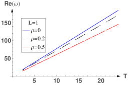
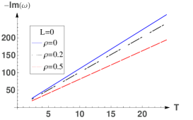
Figure 2: Scalar quasinormal modes vs. temperature of Hořava-Lifshitz spherical black hole spacetime, where $T=\frac{1+3r_{0}}{4\pi}$

We show in Figs.(1, 2) the results obtained by using Horowitz-Hubeny method. By adopting the natural units, namely, $c=\hbar=G=k_{B}=1$, we express all physical quantities in terms of “MeV”. Therefore the units of temperature and frequency are both “MeV”. In the Fig.1 are shown the quasinormal modes for the planar black hole with $T=\frac{3r_{0}}{4\pi}$, while in Fig.(2) are presented the quasinormal modes for the spherical black hole where $T=\frac{1+3r_{0}}{4\pi}$. It is found, from the above figures, that the quasinormal modes are mostly linear with respect to the temperature. However, the slope of the line is affected by the correction (in terms of $\rho$) of Hořava-Lifshitz theory. In particular, the correction increases the imaginary part of the frequency, but suppresses the real part. Compared with the results obtained in general relativity, the quasinormal mode in Hořava-Lifshitz black holes have bigger period of quasinormal oscillation while its amplitude decays more slowly.

We summarize the quasinormal modes for the massless scalar field for some values of $L$ into Table 1.

Table 1: The relation between $L$ and frequencies of Hořava-Lifshitz planar and spherical black hole spacetime with $\rho=0.1$ and $r_{0}=10$.

$L$	$\omega$ (Planar Black Hole)	$\omega$ (Spherical Black Hole)
$0$	$17.8504-25.4472i$	$17.9597-25.4498i$
$1$	$17.9356-25.4244i$	$18.0446-25.4270i$
$2$	$18.1873-25.3571i$	$18.2122-25.3818i$
$3$	$18.5956-25.2492i$	$18.4594-25.3158i$
$4$	$18.9624-24.8185i$	$18.7814-25.2307i$

We note that the smallest frequency occurs at $L=0$, which decays faster than the higher modes. A similar behaviour was pointed out by Horowitz and Hubeny in HH . The imaginary part of the quasinormal modes are smaller in the planar black hole than in the spherical black hole. The real part of the quasinormal modes increases faster for the planar black hole than the spherical black hole after $L=2$.

V Temporal Evolution

In this section, we employ the finite difference method FD to study the temporal evolution of the quasinormal modes in the Hořava-Lifshitz black holes. In this approach, one directly observes how small perturbations evolve in time. To achieve this, we apply the finite difference method to Eq.(3.6) and conveniently rescale the time, so that Eq.(3.6) can now be rewritten as

$$\frac{\partial^{2}\Phi}{\partial{r_{*}^{2}}}-\frac{\partial^{2}\Phi}{\partial t^{2}}=V(r)\Phi.$$ (5.1)

By taking $t=t_{0}+i\Delta t$ and $r_{*}=r_{*0}+j\Delta r_{*}$ in Eq.(5.1), the resulting finite difference equation reads

$$\Phi^{i+1}_{j} = -\Phi^{i-1}_{j}+\frac{\Delta t^{2}}{\Delta r_{*}^{2}}\left(\Phi^{i}_{j-1}+\Phi^{i}_{j+1}\right)$$ (5.2)

$$+\left(2-2\frac{\Delta t^{2}}{\Delta r_{*}^{2}}-\Delta t^{2}V_{j}\right)\Phi^{i}_{j}.$$

The initial conditions are chosen to be

$$\Phi(r_{*},t_{0})=C_{A}\exp(-C_{a}(r_{*}-C_{b})^{2}),$$

$$\frac{\partial}{\partial t}\Phi(r_{*},t)\Big{|}_{t=t_{0}}=0,$$ (5.3)

and the Dirichlet conditions at the Anti-de Sitter boundary is $\Phi(r_{*},t)|_{r_{*}=0}=0$. In order to satisfy the Von Neumann stability

$$\frac{\Delta t^{2}}{\Delta r_{*}^{2}}+\frac{\Delta t^{2}}{4}V_{max}<1,$$ (5.4)

we choose $\Delta r_{*}=2\Delta t$, and $V_{max}\Delta t^{2}<3$, where $V_{max}$ is the largest value of $V_{j}$ in the numerical grids.

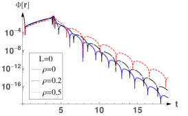
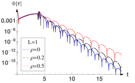
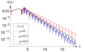
Figure 3: The time evolutions of scalar perturbations in Hořava-Lifshitz planar black hole spacetime for $r_{0}=1$.

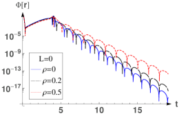
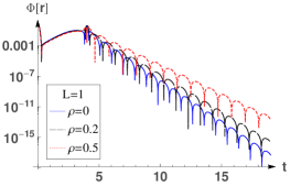
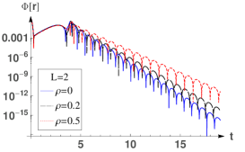
Figure 4: The time evolutions of scalar perturbations in Hořava-Lifshitz spherical black hole spacetime for $r_{0}=1$.

The numerical results are presented in Figs.(3, 4). From the above plots, one may draw the same conclusion that the effect of the Hořava-Lifshitz spacetime is to increase the period of the quasinormal oscillation and its magnitude decays more slowly.

VI Instability at large $\rho$

At last, we study numerically the stability of the scalar field perturbation in Hořava-Lifshitz spacetime in terms of $\rho$. The results shown in Fig.(5) indicate that when $\rho$ becomes large enough, small perturbation may lead to instability of the system. $\rho_{c}$, the critical value of $\rho$, is found numerically for a black hole with $r_{0}=1$ and $L=0$. For planar black hole $\rho_{c}=0.802$ and for spherical black hole $\rho_{c}=0.808$. Thus, in order to preserves the stability of the black holes against massless scalar perturbations, $\rho$ must be smaller than those critical values.

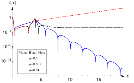
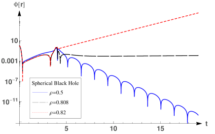
Figure 5: Instability in planar and spherical black hole spacetime, for given $r_{0}=1$ and $L=0$.

Now we proceed to study the frequencies of the quasi normal modes for the unstable region $\rho\geq\rho_{c}$. For such region, one encounters some difficulties in terms of computational time when utilizing the Horowitz-Hubeny method to evaluate the quasinormal mode frequencies. This is because in numerical calculations, one has to choose an integer $n_{N}$ as the number of terms used in the expansion of Eq.(4.6). This integer must be large enough so that the calculated frequency does not depend on the choice of $n_{N}$. However, when $\rho$ increases and approaches its critical value $\rho_{c}$ from below, the minimal value of $n_{N}$ required for obtaining a convergent result tends to increase till the point that sometimes the numerical calculation becomes infeasible. In Fig.6, we illustrate this fact by showing the relation between $n_{N}$ used in the calculation and the resultant $\rho_{c}$.

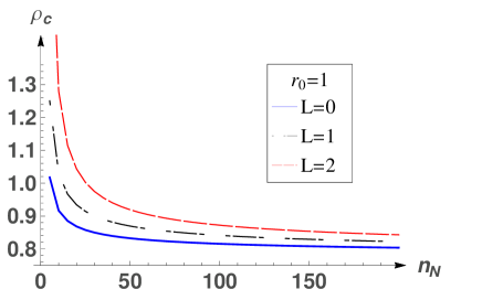
Figure 6: The relation between the number of terms used in the expansion $n_{N}$ and the value of critical $\rho_{c}$ in planar (left hand side) and spherical (right hand side) black hole spacetime, for given $r_{0}=1$. The calculations are carried out by assuming $\omega=0$ for critical case.

Since for the critical mode, one has $\omega=0$, we utilize this information to calculate the corresponding $\rho_{c}$. Numerically, the calculation becomes less time consuming when one makes use of this condition, though it is also possible to study the quasi normal mode without assuming $\omega=0$. Since the calculation becomes very slow with large $n_{N}$, we will adopt the smallest possible value of $n_{N}$ while still achieving a reasonably good convergence. From Fig.6, we find when $n_{N}\geq 50$, the results for $\rho_{c}$ become reasonable close to their convergent values. Therefore we adopt $n_{N}=50$ in the following to evaluate the frequencies for critical as well as unstable modes.

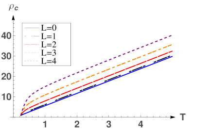
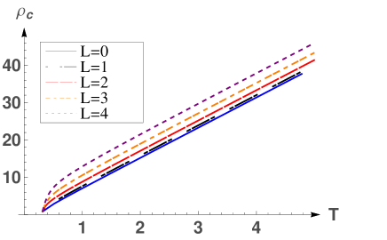
Figure 7: The relation between the critical value $\rho_{c}$ and the temperature $T$ for planar (left hand side, $T=\frac{3r_{0}}{4\pi}$) and spherical (right hand side, $T=\frac{1+3r_{0}}{4\pi}$) black hole spacetime. For critical mode, the frequency $\omega$ vanishes. The value $n_{N}=50$ is used in the calculations.

In Fig.7, we show the value of $\rho_{c}$ as a function of the temperature $T$. It is found that $T$ and $\rho_{c}$ becomes mostly linear at high temperature (or large $r_{0}$) region. The frequencies of quasi normal modes in the unstable region are shown in Table 2. It is confirmed that the real parts of the frequencies is numerically consistentely with zero in this case, and imaginary parts are positive. Therefore the amplitudes of the oscillations are divergent when time goes to infinity, in accordance with the physical interpretation.

Table 2: The relation between $\rho$ and frequencies of the unstable quasi normal modes in Hořava-Lifshitz planar and spherical black hole spacetime with $L=0$ and $r_{0}=1$. The number of terms in the expansion is $n_{N}=50$

$\rho$	$\omega$ (Planar Black Hole)	$\omega$ (Spherical Black Hole)
$0.85$	$0.570335i$	$0.241044i$
$0.9$	$2.20793i$	$2.15592i$
$0.95$	$4.08224i$	$4.07901i$

VII Conclusion

In this work, we obtain the planar and spherical black hole solutions of Hořava-Lifshitz Gravity with local $U(1)$ symmetry, and investigate the massless scalar quasinormal modes in these spacetimes. We find that the effect of Hořava-Lifshitz correction is to increases the period of quasinormal oscillation and slowing down the exponential decay. Moreover, the scalar field’s evolution will make the black hole unstable when $\rho$ becomes larger than a critical value. The frequencies for critical and unstable modes are also evaluated.

As mentioned in UH , even in the IR limit, some theory may still allow the existence of massless particles with velocity exceeding that of the light. For example, due to the presence of spin-0 and spin-1 gravitons in Einstein-aether theoryEA , it is required that these particles should propagate with a velocity no less than that of the light, in order to cancel the Cherenkov effectsEMS .

On the other hand, in UV case, Hořava-Lifshitz gravity allows the existence of particles with infinite velocity. Our recent studies on universal horizon show that even particles with arbitrarily large velocities cannot escape from the inside of the universal horizonUH ; UHmore . This implies that the universal horizon, which situates inside of the event horizon, may play the role of a real horizon of the black hole in a theory without Lorentz symmetry. In this paper, we focus on low energy phenomena by ignoring the higher energy terms in the action of the scalar field. In this context, the boundary condition at event horizon shall be valid, in other words, the event horizon plays the role of black hole horizon.

We plan to investigate the quasinormal modes of Hořava-Lifshitz black hole in UV limit. In this case, the black hole should be defined by the universal horizon. In the UV limit, the Horowitz-Hubeny method shall be modified accordingly because the condition of a pure in-going mode at killing event horizon ceases to be valid; while the finite difference method in Anti-de Sitter black hole spacetime still works. In fact, in the finite difference method, we find that the calculated perturbation won’t reach the killing event horizon, which situates outside of the universal horizon. Nonetheless, besides the finite difference method, it is a challenging and intriguing task to further develop other methods in order to study the properties of quasinormal modes of Hořava-Lifshitz black hole in the UV limit.

Nevertheless, it is interesting to investigate the quasinormal modes of the matter field by taking into account those higher energy terms in Hořava-Lifshitz theory. It is also compelling to investigate the gravitational perturbation, which in turn helps to understand the stability of the black holes and the properties of the gravitational wave in Hořava-Lifshitz theory. We will devote ourselves to these topics in the future.

VIII Appendix: Projectable Planar Black Hole Solutions

In the Appendix, we derive a planar black hole solution with projectability condition and $U(1)$ symmetry. The projectable total action can be written as HLALW ; HLHW ,

$$S = \zeta^{2}\int dtd^{3}xN\sqrt{g}\Big{(}{\cal{L}}_{K}-{\cal{L}}_{{V}}+{\cal{L}}_{{\varphi}}+{\cal{L}}_{{A}}+{\cal{L}}_{{\lambda}}$$ (A.1)

$$~{}~{}~{}~{}~{}~{}~{}~{}~{}~{}~{}~{}~{}~{}~{}~{}~{}~{}~{}~{}~{}~{}\left.+{\zeta^{-2}}{\cal{L}}_{M}\right),$$

where ${\cal{L}}_{K},\;{\cal{L}}_{\varphi}$ and ${\cal{L}}_{A}$ are given by Eq.(II) with $a_{i}=0$, and the potential ${\cal{L}}_{{V}}$ reads

$${\cal{L}}_{{V}} = 2\Lambda+g_{1}R+\frac{1}{\zeta^{2}}\left(g_{2}R^{2}+g_{3}R_{ij}R^{ij}\right)$$ (A.2)

$$+\frac{1}{\zeta^{4}}\left(g_{4}R^{3}+g_{5}R\;R_{ij}R^{ij}+g_{6}R^{i}_{j}R^{j}_{k}R^{k}_{i}\right)$$

$$+\frac{1}{\zeta^{4}}\Big{[}g_{7}(\nabla R)^{2}+g_{8}\left(\nabla_{i}R_{jk}\right)\left(\nabla^{i}R^{jk}\right)\Big{]},~{}~{}~{}~{}$$

where the coupling constants $g_{s}\,(s=1,2,\dots 8)$ are all dimensionless, and we set $g_{1}=-1$ in the following calculations (In fact, we find the form of ${\cal L}_{V}$ only influences the solution of $A(r)$ in spherically symmetric spacetime).

The planar black hole metric is given by

$$ds^{2}=-N^{2}dt^{2}+\frac{\left[dr+h(r)dt\right]^{2}}{f(r)}+r^{2}(dx^{2}+dy^{2}),$$ (A.3)

since the projectability condition requires $N=N(t)$, we set $N=1$ without loss the generality. Subsequently, the field equations can be derived from the action (A.1) HLALW . We pick the gauge $\varphi=0$, and obtain the following field equations

$$rf^{\prime}+f+\Lambda_{g}r^{2}=0,$$ (A.4)

$$(\lambda-1)\left[h^{\prime\prime}+\left(\frac{2}{r}-\frac{f^{\prime}}{2f}\right)h^{\prime}\right]+\frac{f^{\prime}h}{rf}$$

$$+(\lambda-1)\left(\frac{f^{\prime 2}}{2f^{2}}+\frac{f^{\prime\prime}}{2f}-\frac{2}{r^{2}}\right)h = 0,$$ (A.5)

$$A^{\prime}+\left(\frac{1}{r}+\frac{r\Lambda_{g}}{f}\right)\frac{A^{\prime}}{2}-\frac{\Lambda r^{2}+f}{2rf}+\frac{hh^{\prime}}{f}$$

$$+\left(\frac{1}{2rf}-\frac{f^{\prime}}{f^{2}}\right)h^{2}+(\lambda-1)\Bigg{[}\frac{rh^{\prime 2}}{4f}-\frac{rhh^{\prime\prime}}{2f}$$

$$+\left(\frac{2}{rf}-\frac{f^{\prime}}{2f^{2}}-\frac{3rf^{\prime 2}}{16f^{3}}+\frac{rf^{\prime\prime}}{4f^{2}}\right)h^{2}\Bigg{]}+Q(r)=0,$$

where $Q(r)$ is higher energy term, which is given by

$$Q(r) = \frac{(8g_{2}+3g_{3})(r^{2}\Lambda_{g}+2f)r^{2}\Lambda_{g}-g_{3}f^{2}}{8\xi^{2}r^{3}f}$$ (A.7)

$$+\frac{1}{8\xi^{4}r^{5}f}\Big{[}(32g_{4}+12g_{5}+5g_{6}-g_{8})\Lambda_{g}^{3}r^{6}$$

$$+(48g_{4}+14g_{5}+3g_{6}+2g_{8})\Lambda_{g}^{2}r^{4}f$$

$$-(40g_{4}+45g_{6}-35g_{8})\Lambda_{g}r^{2}f^{2}$$

$$-(66g_{5}+75g_{6}-60g_{8})f^{3}\Big{]}$$

From Eq.(A.4), we get

$$f(r)=\frac{f_{0}}{r}-\frac{\Lambda_{g}}{3}r^{2},$$ (A.8)

where $f_{0}$ is a constant. Then, one can use Eq.(VIII) and Eq.(VIII) to calculate $h(r)$ and $A(r)$.

VIII.1 $\lambda=1$ Case

When $\lambda=1$, from Eq.(VIII), we have $h(r)=0$. By substituting $h=0$ into Eq.(VIII), one obtains

$$A(r) = \sqrt{f(r)}A_{0}+\frac{\Lambda}{\Lambda_{g}}-\frac{3\left(22g_{5}+25g_{6}-20g_{8}\right)f(r)^{2}}{44\xi^{4}r^{4}}$$ (A.9)

$$-\Lambda_{g}\left[\frac{242g_{5}+270g_{6}-205g_{8}}{220\xi^{4}r^{2}}f+\frac{8g_{2}+3g_{3}}{4\xi^{2}}\right]$$

$$-\frac{g_{3}f}{20\xi^{2}r^{2}}+\frac{\left(-32g_{4}-12g_{5}-5g_{6}+g_{8}\right)\Lambda_{g}^{2}}{4\xi^{4}}$$

$$-A_{S}(r)\Big{[}\frac{2\left(110g_{4}+44g_{5}+20g_{6}-5g_{8}\right)\Lambda_{g}^{3}}{55\xi^{4}}$$

$$+\frac{2\left(5g_{2}+2g_{3}\right)\Lambda_{g}^{2}}{5\xi^{2}}-\Lambda_{g}+\Lambda\Big{]}$$

where $A_{0}$ is a constant, and

$$A_{S}(r)=\frac{i(-1)^{5/12}f_{0}^{1/2}f(r)^{1/2}}{3^{1/12}(-f_{0})^{5/6}(-\Lambda_{g})^{7/6}}$$

$$\times F\left[\arcsin\left(3^{-\frac{1}{4}}\sqrt{-(-1)^{\frac{5}{6}}-\frac{i3^{\frac{1}{3}}(-f_{0})^{\frac{1}{3}}}{r(-\Lambda_{g})^{\frac{1}{3}}}}\right)\Bigg{|}(-1)^{\frac{1}{3}}\right],$$

and $F(\phi|m)=\int^{\phi}_{0}[1-m\sin^{2}(\theta)]^{-1/2}d\theta$ is the elliptic integral.

In particular, when $\Lambda=\Lambda_{g}$ and $g_{i}=0$, we find

$$A(r)=1+A_{0}\sqrt{f(r)}$$ (A.11)

where $A_{0}$ is a constant.

VIII.2 $\lambda\not=1$ and $f_{0}=0$ Case

In this case, we find

$$h = h_{1}r^{\sqrt{\frac{\lambda-3}{\lambda-1}}}+h_{2}r^{-\sqrt{\frac{\lambda-3}{\lambda-1}}},$$

$$A = A_{0}r-\frac{1}{2}+\frac{3\Lambda}{2\Lambda_{g}}-\frac{2\Lambda_{g}^{2}}{3\xi^{4}}(9g_{4}+3g_{5}+g_{6})$$ (A.12)

$$-\frac{\Lambda_{g}}{3\xi^{2}}(3g_{2}+g_{3})+\frac{3h_{1}^{2}}{2\Lambda_{g}r^{2\left(1+\sqrt{\frac{\lambda-3}{\lambda-1}}\right)}}$$

$$\times\Bigg{[}\frac{\sqrt{(\lambda-1)^{3}(\lambda-3)}+2\sqrt{(\lambda-1)(\lambda-3)}}{3\sqrt{\lambda-1}+2\sqrt{\lambda-3}}$$

$$-\frac{(\lambda-1)(\lambda-3)}{3\sqrt{\lambda-1}+2\sqrt{\lambda-3}}\Bigg{]}+\frac{3h_{2}^{2}}{2\Lambda_{g}r^{2\left(-1+\sqrt{\frac{\lambda-3}{\lambda-1}}\right)}}$$

$$\times\Bigg{[}\frac{\sqrt{(\lambda-1)^{3}(\lambda-3)}+2\sqrt{(\lambda-1)(\lambda-3)}}{-3\sqrt{\lambda-1}+2\sqrt{\lambda-3}}$$

$$+\frac{(\lambda-1)(\lambda-3)}{-3\sqrt{\lambda-1}+2\sqrt{\lambda-3}}\Bigg{]}$$

where $h_{1}$ and $h_{2}$ are constants.

VIII.3 $\lambda\not=1$ and $\Lambda_{g}=0$ Case

In this case, we find

$$h = h_{1}r^{-\frac{3}{4}-\Lambda_{C}}+h_{2}r^{-\frac{3}{4}+\Lambda_{C}},$$

$$A = \frac{A_{0}}{\sqrt{r}}+1+\frac{\Lambda r^{3}}{7f_{0}}+\frac{h_{2}^{2}}{8f_{0}r^{\frac{1}{2}+2\Lambda_{C}}}\left(\frac{1}{\Lambda_{C}}-4\right)$$ (A.13)

$$-\frac{h_{1}^{2}}{8f_{0}r^{\frac{1}{2}+2\Lambda_{C}}}\left(\frac{1}{\Lambda_{C}}+4\right)+\frac{h_{1}h_{2}\ln(r)}{2f_{0}\sqrt{r}}$$

$$-\frac{3f_{0}^{2}}{44\xi^{4}r^{6}}(22g_{5}+25g_{6}-20g_{8})-\frac{g_{3}f_{0}}{20\xi^{2}r^{3}}$$

$$+\frac{\lambda-1}{128f_{0}r^{\frac{1}{2}+2\Lambda_{C}}}\Big{[}4h_{1}h_{2}r^{2\Lambda_{C}}(49-\Lambda_{C}^{2})\ln(r)$$

$$+\left(48\Lambda_{C}-56-\frac{49}{\Lambda_{C}}\right)h_{1}^{2}$$

$$-\left(48\Lambda_{C}+56-\frac{49}{\Lambda_{C}}\right)h_{2}^{2}r^{4\Lambda_{C}}\Big{]},$$

where $\Lambda_{C}=\frac{1}{4}\sqrt{\frac{49\lambda-33}{\lambda-1}}$.

VIII.4 General Case

In a general case, $A(r)$ should be obtained from Eq.(VIII), namely,

$$A(r)=A_{0}\sqrt{f}-\sqrt{f}\int\frac{Q_{A}(r)}{\sqrt{f}}dr,$$ (A.14)

where

$$Q_{A}(r) = Q(r)-\frac{\Lambda r^{2}+f}{2rf}+\frac{hh^{\prime}}{f}$$ (A.15)

$$+\left(\frac{1}{2rf}-\frac{f^{\prime}}{f^{2}}\right)h^{2}+(\lambda-1)\Bigg{[}\frac{rh^{\prime 2}}{4f}-\frac{rhh^{\prime\prime}}{2f}$$

$$+\left(\frac{2}{rf}-\frac{f^{\prime}}{2f^{2}}-\frac{3rf^{\prime 2}}{16f^{3}}+\frac{rf^{\prime\prime}}{4f^{2}}\right)h^{2}\Bigg{]}.$$

To calculate $h(r)$, one makes use of Eq.(VIII). We introduce the following transformation

$$x = \frac{\Lambda_{g}^{1/3}r}{3^{1/3}f_{0}^{1/3}},$$

$$h = x^{\frac{2c-5}{4}(1-x^{3})^{\frac{3+2b-2c}{12}}}H(x),$$ (A.16)

and Eq.(VIII) becomes

$$x(1-x^{3})H^{\prime\prime}(x)+(c-bx^{3})H^{\prime}(x)+ax^{2}H(x)=0$$

where the $a$, $b$ and $c$ may be given by

$$a = \frac{3+21\lambda}{8-8\lambda}-\frac{3}{2}\Lambda_{C},~{}~{}b=\frac{5}{2}+2\Lambda_{C},$$

$$c = 1+2\Lambda_{C},$$ (A.18)

or

$$a = \frac{33-57\lambda}{8\lambda-8}-\frac{9}{2}\Lambda_{C},~{}~{}b=\frac{11}{2}+2\Lambda_{C},$$

$$c = 1+2\Lambda_{C},$$ (A.19)

or

$$a = \frac{3+21\lambda}{8\lambda-8}+\frac{3}{2}\Lambda_{C},~{}~{}b=\frac{5}{2}-2\Lambda_{C},$$

$$c = 1-2\Lambda_{C},$$ (A.20)

or

$$a = \frac{33-57\lambda}{8\lambda-8}+\frac{9}{2}\Lambda_{C},~{}~{}b=\frac{11}{2}-2\Lambda_{C},$$

$$c = 1-2\Lambda_{C},$$ (A.21)

If we set $y=x^{3}$, Eq.(VIII.4) becomes a hypergeometric equation

$$y(1-y)\frac{d^{2}H}{dy^{2}}+\frac{1}{3}\left[2+c-(2+b)y\right]\frac{dH}{dy}+\frac{a}{9}H=0,$$

and the solution is

$$H = \frac{h_{1}}{y^{\frac{1-c}{3}}}~{}~{}{}_{2}F_{1}\left(H_{A-},H_{A+};\frac{4-c}{3};y\right)$$ (A.23)

$$+h_{2}~{}~{}{}_{2}F_{1}\left(H_{B-},H_{B+};\frac{2+c}{3};y\right),$$

$$= \frac{h_{1}}{x^{1-c}}~{}~{}{}_{2}F_{1}\left(H_{A-},H_{A+};\frac{4-c}{3};x^{3}\right)$$

$$+h_{2}~{}~{}{}_{2}F_{1}\left(H_{B-},H_{B+};\frac{2+c}{3};x^{3}\right),$$

where $H_{A\pm}=\frac{b+1}{6}-\frac{c}{3}\pm\frac{1}{6}\sqrt{4a+b^{2}-2b+1}$, $H_{B\pm}=\frac{b-1}{6}\pm\frac{1}{6}\sqrt{4a+b^{2}-2b+1}$, and ${}_{2}F_{1}(a,b;c;d)$ is the hypergeometric function.

References

(1) P. Hořava, Phys. Rev. D79, 084008 (2009) arXiv:0901.3775
(2) P. Hořava and C. M. Melby-Thompson, Phys. Rev. D 82, 064027 (2010) arXiv:1007.2410
(3) A. Wang, Phys. Rev. D 82, 124063 (2010) arXiv:1008.3637; S. Mukohyama, J. Cosmol. Astropart. Phys., 06, 001 (2009) arxiv:0904.2190.
(4) T. Zhu, F.-W. Shu, Q. Wu, and A. Wang, Phys. Rev. D 85, 044053 (2012) arXiv:1110.5106;A. Wang and Y. Wu, Phys. Rev. D83, 044031 (2011) arXiv:1009. 2089; K. Lin, A. Wang, Q. Wu, and T. Zhu, Phys. Rev. D84, 044051 (2011) arXiv:1106.1486.
(5) K. Lin, S. Mukohyama and A. Wang, Phys. Rev. D 86, 104024 (2012) arXiv:1206.1338; K. Lin and A. Wang, Phys. Rev. D87, 084041 (2013) arXiv:1212.6794
(7) S.J. Zhang, Q. Pan, B. Wang and E. Abdalla JHEP 1309 (2013) 101.
(8)E. Abdalla, C.E. Pellicer, J. de Oliveira and A B. Pavan Phys.Rev. D82 (2010) 124033.
(9) T. Zhu, Q. Wu, A. Wang, and F.-W. Shu, Phys. Rev. D84, 101502 (R) (2011) arXiv:1108.1237
(10) K. Lin, S. Mukohyama, A. Wang and T. Zhu, Phys. Rev. D89, 084022 (2014) arXiv:1310.6666
(11) A. Borzou, K. Lin, and A. Wang, J. Cosmol. Astropart. Phys., 05, 006 (2011) arXiv:1103.4366
(12) Y.-Q. Huang, and A. Wang, Phys. Rev. D83, 104012 (2011) arXiv:1011.0739
(13) G.T. Horowitz, V. E. Hubeny, Phys. Rev. D62, 024027 (2000) arXiv:hep-th/9909056
(14) B. Cuadros-Melgar, J. de Oliveira, C. E. Pellicer, Phys. Rev. D85, 024014 (2012) arXiv:1110.4856; E. Abdalla, O. P. F. Piedra, F. S. Nuñez, J. de Oliveira, 88, 064035 (2013) arXiv:1211.3390; B. Cuadros-Melgar, J. de Oliveira, C.E. Pellicer, J. Phys. Conf. Ser. 453, 012025 (2013) arXiv:1302.6185
(15) K. Lin, E. Abdalla, R. G. Cai and A. Wang, Int. J. Mod.
Phys. D 23, 1443004 (2014);
(16) T. Jacobson and D. Mattingly, Phys. Rev. D 64, 024028
(2001); T. Jacobson, Proc. Conf. from Quantum to Emergent Gravity:
Theory and Phenomenology, Vol. 020 (2007), arXiv:0801.1547.
(17) J. W. Elliott, G. D. Moore and H. Stoica, J. High Energy Phys. 08, 066
(2005) arXiv:hep-ph/0505211
(18) K. Lin, O. Goldoni, M. F. da Silva and A. Wang, Phys. Rev. D 91, 024047 (2015);
K. Lin, F.-W. Shu, A. Wang, and Q. Wu, Phys. Rev. D91, 044003
(2015); K. Lin, V. H. Satheeshkumar and A. Wang, Phys. Rev. D 93,
124025 (2016).