Extracting Flexibility of Heterogeneous Deferrable Loads via Polytopic Projection Approximation

Abstract

Aggregation of a large number of responsive loads presents great power flexibility for demand response. An effective control and coordination scheme of flexible loads requires an accurate and tractable model that captures their aggregate flexibility. This paper proposes a novel approach to extract the aggregate flexibility of deferrable loads with heterogeneous parameters using polytopic projection approximation. First, an exact characterization of their aggregate flexibility is derived analytically, which in general contains exponentially many inequality constraints with respect to the number of loads. In order to have a tractable solution, we develop a numerical algorithm that gives a sufficient approximation of the exact aggregate flexibility. Geometrically, the flexibility of each individual load is a polytope, and their aggregation is the Minkowski sum of these polytopes. Our method originates from an alternative interpretation of the Minkowski sum as projection. The aggregate flexibility can be viewed as the projection of a high-dimensional polytope onto the subspace representing the aggregate power. We formulate a robust optimization problem to optimally approximate the polytopic projection with respect to the homothet of a given polytope. To enable efficient and parallel computation of the aggregate flexibility for a large number of loads, a muti-stage aggregation strategy is proposed. The scheduling policy for individual loads is also derived. Finally, an energy arbitrage problem is solved to demonstrate the effectiveness of the proposed method.

I Introduction

The future power system will be modernized with advanced metering infrastructure, bilateral information communication network, and intelligent monitoring and control system to enable a smarter operation [5]. The transformation to the smart grid is expected to facilitate the deep integration of renewable energy, improve the reliability and stability of the power transmission and distribution system, and increase the efficiency of power generation and energy consumption.

Demand response program is a core subsystem of the smart grid, which can be employed as a resource option for system operators and planners to balance the power supply and demand. The demand side control of responsive loads has attracted considerable attention in recent years [7, 19, 18, 31]. An intelligent load control scheme should deliver a reliable power resource to the grid, while maintaining a satisfactory level of power usage to the end-user. One of the greatest technical challenges of engaging responsive loads to provide grid services is to develop control schemes that can balance the aforementioned two objectives [8]. To achieve such an objective, a hierarchical load control structure via aggregators is suggested to better integrate the demand-side resources into the power system operation and control [27, 8].

In the hierarchical scheme, the aggregator performs as an interface between the loads and the system operator. It aggregates the flexibility of responsive loads and offers it to the system operator. In the meantime, it receives dispatch signals from the system operator, and execute appropriate control to the loads to track the dispatch signal. Therefore, an aggregate flexibility model is fundamentally important to the design of a reliable and effective demand response program. It should be detailed enough to capture the individual constraints while simple enough to facilitate control and optimization tasks. Among various modeling options for the adjustable loads such as thermostatically controlled loads (TCLs), the average thermal battery model [15, 32, 24, 18] aims to quantify the aggregate flexibility, which is the set of the aggregate power profiles that are admissible to the load group. It offers a simple and compact model to the system operator for the provision of various ancillary services. Apart from the adjustable loads, deferrable loads such as pools and plug-in vehicles (PEVs) can also provide significant power flexibility by shifting their power demands to different time periods. However, different from the adjustable loads, it is more difficult to characterize the flexibility of deferrable loads due to the heterogeneity in their time constraints.

In this paper, we focus on modeling the aggregate flexibility for control and planning of a large number of deferrable loads. There is an ongoing effort on the characterization of the aggregate flexibility of deferrable loads [26, 20, 14, 10]. An empirical model based on the statistics of the simulation results was proposed in [20]. A necessary characterization was obtained in [26] and further improved in [14]. For a group of deferrable loads with homogeneous power, arrival time, and departure time, a majorization type exact characterization was reported in [14]. With heterogeneous departure times and energy requirements, a tractable sufficient and necessary condition was obtained in [10], and was further utilized to implement the associated energy service market [9]. Despite these efforts, a sufficient characterization of the aggregate flexibility for general heterogeneous deferrable loads remains a challenge.

To address this issue, we propose a novel geometric approach to extract the aggregate flexibility of heterogeneous deferrable loads. Geometrically, the aggregate flexibility modeling amounts to computing the Minkowski sum of multiple polytopes, of which each polytope represents the flexibility of individual load. However, calculating the Minkowski sum of polytopes under facet representation is generally NP-hard [29]. Interestingly, we are able to show that for a group of loads with general heterogeneity, the exact aggregate flexibility can be characterized analytically. But the problem remains in the sense that there are generally exponentially many inequalities with respect to the number of loads and the length of the time horizons, which can be intractable when the load population size or the number of steps in the considered time horizon is large. Therefore, a tractable characterization of the aggregate flexibility is desired.

For deferrable loads with heterogeneous arrival and departure times, the constraint sets are polytopes that are contained in different subspaces. Alternative to the original definition of the Minkowski sum, we find it beneficial to regard it as a projection operation. From the latter perspective, the aggregate flexibility is considered as the projection of a higher dimensional polytope to the subspace representing the aggregate power of the deferrable loads. Therefore, instead of approximating the Minkowski sum directly by its definition, we turn to approximating the associated projection operation. To this end, we formulate an optimization problem which approximates the projection of a full dimensional polytope via finding the maximum homothet of a given polytope, i.e., the dilation and translate of that polytope. The optimization problem can be solved very efficiently by solving an equivalent linear program. Furthermore, we propose a “divide and conquer” strategy which enables efficient and parallel computation of the aggregate flexibility of the load group. The scheduling policy for each individual load is derived simultaneously along the aggregation process. Finally, we apply our model to the PEV energy arbitrage problem, where given predicted day-ahead energy prices, the optimal power profile consumed by the load group is calculated to minimize the total energy cost. The simulation results demonstrate that our approach is very effective at characterizing the feasible aggregate power flexibility set, and facilitating finding the optimal power profile.

There are several closely-related literature on characterizing flexibility of flexible loads. In our previous work [32], a geometric approach was proposed to optimally extract the aggregate flexibility of heterogeneous TCLs based on the given individual physical models. The simulation demonstrated accurate characterization of the aggregate flexibility which was very close to the exact one. However, this approach cannot be applied to the deferrable loads directly. Similar to [32] which sought a special class of polytopes to facilitate fast calculation of Minkowski sum, the authors in [25] proposed to characterize the power flexibility using Zonotopes. Different from [32], this method could deal with the time heterogeneity as appeared in the deferrable loads. In addition, both approaches extracted the flexibility of individual load. In comparison, the approach proposed in this paper is a batch processing method: it directly approximates the aggregate flexibility of a group of loads, which could mitigate the losses caused by the individual approximation as emphasized in [25].

Notation: The facet representation of a polytope $\mathcal{P}\subset\mathbb{R}^{m}$ is a bounded solution set of a system of finite linear inequalities [16]: $\mathcal{P}:=\{x:Ax\leq c\}$, where throughout this paper $\leq$ (or $<$, $\geq$, $>$) means elementwise inequality. A polytope $\mathcal{P}\subset\mathbb{R}^{m}$ is called full dimensional, if it contains an interior point in $\mathbb{R}^{m}$. Given a full dimensional polytope $\mathcal{P}$ in $\mathbb{R}^{m}$, a scale factor $\lambda>0$, and a translate factor $\mu\in\mathbb{R}^{m}$, the set $\lambda\mathbb{B}+\mu$ is called a homothet of $\mathbb{B}$. We use $\biguplus$ to denote the Minkowski sum of multiple sets, and $\oplus$ of two sets. We use ${\bf 1}_{m}$ to represent the $m$ dimensional column vector of all ones, $I_{m}$ the $m$ dimensional identity matrix, and $\mathbbm{1}_{C}$ the indicator function of the set $C$. The bold $\mathbf{0}$ denotes the column vector of all $0$’s with appropriate dimension. For two column vectors $u$ and $v$, we write $(u,v)$ for the column vector $[u^{T},v^{T}]^{T}$ where no confusion shall arise.

II Problem Formulation

We consider the problem of charging a group of $N$ PEVs. The energy state of each PEV can be described by a discrete time difference equation on a finite time horizon $[0,T\delta]$,

$$x_{t}=x_{t-1}+\delta u_{t},$$ (1)

where $x_{t}$ is the state of charge (SoC) with initial condition $x_{0}=0$, and $u_{t}\in[0,p]$ with $p>0$ is the charging power supplied to the vehicle during $[(t-1)\delta,t\delta)$. Let $t\in\mathrm{\mathbb{T}}:=\{1,2,\dots m\}$ denote the time interval $[(t-1)\delta,t\delta)$, where without loss of generality, we will assume the time unit $\delta=1$ hour in the sequel. Moreover, the PEV must be charged during a time window $\mathbb{A}:=\{a,\dots,d\}\subset\mathrm{\mathbb{T}}$ where $a$ is its arrival time, $d$ is its departure time, and $a<d$.. At the deadline $d$, the PEV is supposed to be charged with an SoC $x_{d}\in[\underline{E},\bar{E}]$, where we assume that $\bar{E}^{i}>\underline{E}^{i}$. The load is called deferrable if $\bar{E}<(d-a)p$. A charging power profile $u:=[u_{1},\dots,u_{m}]^{T}$ is called admissible if the load is only charged within $\mathbb{\mathbb{A}}$ and its SoC at $t=m$ is within $[\underline{E},\bar{E}]$.

We differentiate the $i^{\mbox{th}}$ PEV ($\forall i\in\mathcal{N}:=\{1,2,\cdots,N\}$) by using a superscript $i$ on the variables introduced above. The charging task of the $i^{\mbox{th}}$ PEV is determined by $\Omega^{i}:=\{a^{i},d^{i},p^{i},\underline{E}^{i},\bar{E}^{i}\}$. Let $\mathcal{P}^{i}$ be the set of all the admissible power profiles of the $i^{\mbox{th}}$ load. It can be described as,

$$\mathcal{P}^{i}:=\left\{\begin{array}[]{l}u^{i}\in\mathbb{R}^{m}:u_{t}^{i}\in[0,p^{i}],\forall t\in\mathbb{A}^{i},\\ u_{t}^{i}=0,\forall i\in\mathrm{\mathbb{T}}\backslash\mathbb{\mathbb{A}}^{i}\mbox{ and }{\bf 1}_{m}^{T}u^{i}\in[\underline{E}^{i},\bar{E}^{i}]\end{array}\right\}$$ (2)

It is straightforward to see that each $\mathcal{P}^{i}$ is a convex polytope. In addition, we say $\mathcal{P}^{i}$ is of codimension $m-\left|\mathbb{A}^{i}\right|$ if its affine hull is a $\left|\mathbb{A}^{i}\right|$ dimensional subspace of $\mathbb{R}^{m}$.

In the smart grid, the aggregator is responsible for procuring a generation profile from the whole market to service a group of loads. We define the generation profile that meets the charging requirements of all PEVs as follows.

Definition 1.

A generation profile $u$ is called adequate if there exists a decomposition $u=\sum_{i=1}^{N}u^{i}$, such that $u^{i}$ is an admissible power profile for the $i^{\mbox{th}}$ load, i.e., $u^{i}\in\mathcal{P}^{i}$.

We call the set of all the adequate generation profiles the aggregate flexibility of the load group. It can be defined as the Minkowski sum of the admissible power sets of each load,

$$\mathcal{P}=\biguplus_{i=1}^{N}\mathcal{P}^{i}:=\left\{u\in\mathbb{R}^{m}:u=\sum_{i=1}^{N}u^{i},~{}u^{i}\in\mathcal{P}^{i}\right\}.$$ (3)

It is straightforward to show that $\mathcal{P}$ is also a convex polytope whose codimension is to be determined by the parameters $\Omega$ of the deferrable loads.

III Exact Characterization of the Aggregate Flexibility

The numerical complexity of the existing algorithms for calculating the Minkowski sum is rather expensive (See [30] for some numerical results). In general, calculating $\mathcal{P}_{1}\oplus\mathcal{P}_{2}$ when $\mathcal{P}_{1}$ and $\mathcal{P}_{2}$ are polytopes specified by their facets is NP-hard [29]. However, for the particular problem of PEV charging, it is possible to characterize the exact aggregate flexibility $\mathcal{P}$ analytically. Such characterization is built on the results from the matrix feasibility problem and from the network flow theory, both of which are intrinsically connected with the PEV charging problem.

Theorem 1.

Consider a group of PEVs or deferrable loads with heterogeneous parameters $\Omega^{i}=\{a^{i},d^{i},p^{i},\underline{E}^{i},\bar{E}^{i}\}$, $i\in\mathcal{N}$. Then the set $\mathcal{P}$ of adequate generation profiles consists of those $u=[u_{1},u_{2},\cdots,u_{m}]^{T}$ which satisfy

$$\min\left\{\sum_{i\in\alpha}\bar{E}^{i}-\sum_{t\in\beta}u_{t},\ \sum_{t\in\mathrm{\beta^{c}}}u_{t}-\sum_{i\in\alpha^{c}}\underline{E}^{i}\right\}\\ \geq-\sum_{i\in\alpha^{c}}\left|\beta\cap\mathbb{A}^{i}\right|p^{i},$$ (4)

for all subsets $\alpha\subset\mathcal{N}$ and $\beta\subset\mathrm{\mathbb{T}}$, where $\alpha^{c}$ and $\beta^{c}$ are the complement sets of $\alpha$ and $\beta$ in $\mathcal{N}$ and $\mathrm{\mathbb{T}}$, respectively.

Proof.

We first interpret the characterization of $\mathcal{P}$ as a matrix feasibility problem. By definition, if a generation profile $u$ is adequate, then there exists a decomposition $u=\sum_{i=1}^{N}u^{i}$ such that $u^{i}$ completes the $i^{\mbox{th}}$ PEV’s charging task. This is equivalent to the existence of a $N\times m$ matrix $M$, the $i^{\mbox{th}}$ row of which is an admissible power profile of the $i^{\mbox{th}}$ PEV. The matrix $M$ will be referred to as the charging matrix. Given $u\in\mathcal{P}$, let $\mathcal{M}(u)$ denote the set of all such charging matrices. These matrices have special structures: the columns indexed by $\mathbb{A}^{i}$ in the $i^{\mbox{th}}$ row are the free positions which can be filled with a real number in $[0,p^{i}]$, while the rest of the positions in this row are forbidden positions that can only be filled with $0$’s. Moreover, $\forall M\in\mathcal{M}(u)$, it has the $t^{\mbox{th}}$ column sum $u_{t}$ and the $i^{\mbox{th}}$ row sum in the interval $[\underline{E}^{i},\bar{E}^{i}]$. Clearly, the non-emptiness of the set gives the condition for being an adequate generation profiles, i.e,

$$\mathcal{P}=\{u\in\mathbb{R}^{m}:\ \mathcal{M}(u)\neq\emptyset\}.$$

Furthermore, the condition for $\mathcal{M}(u)\neq\emptyset$ can be derived by applying [17, Theorem 2.7] to the matrix case. By the definition in [17], partitions $\{r_{1},r_{2},\cdots,r_{N}\}$ and $\{c_{1},c_{2},\cdots,c_{m}\}$ of a sequence are said to be orthogonal, if $\left|r_{i}\cap c_{t}\right|\leq 1$, $\forall i\in\mathcal{N}$ and $\forall t\in\mathrm{\mathbb{T}}$. For a matrix, clearly the rows and columns constitute such orthogonal partitions. This is the only condition required by [17, Theorem 2.7]. Then by a direct calculation of the summation on the right hand side of [17, (2.8)], we can obtain (4). This completes the proof. ∎

Remark 1.

In general, there are $2^{mN+1}$ inequalities in (4), which will be intractable if $N$ is several thousand. When the PEVs are fully homogeneous, i.e., they share the same set of parameters $\Omega$, the above result reduces to the well-known majorization condition [14, 23], which consists of only $N+m$ inequalities. In the linear algebra literature, studies on the matrix feasibility problem are also focused on finding tractable conditions under limited heterogeneities in the parameters. Adapted to the PEV charging scenario, if the arrival time $a$ and the charging rate $p$ are homogeneous, $\underline{E}^{i}=\bar{E}^{i}$, and under certain monotonicity condition on $u$, the number of inequalities in (4) can be significantly reduced [6, 10]. The author in [11] obtained a simple majorization type result under a special monotonicity condition on $u$. Under this condition, the charging rate $p$ can be relaxed to be heterogeneous both among different PEVs and at different time instances. Note that Theorem 1 also applies to the case where the charging rate takes integer values (see [17, Remark (2.19)]).

Since the condition (4) is very difficult to check in practice, the goal of this paper is to find a sufficient approximation of it using much fewer inequalities that does not depend on $N$. The direct approximation from (4) could be difficult. However, it is possible to start with the definition (3). An interesting perspective is to view the Minkowski sum as a projection operation. Clearly, from (3), we see that $\mathcal{P}$ is the projection of a higher dimensional polytope $\tilde{\mathcal{P}}$ onto the $u$ subspace, i.e.

$$\mathcal{P}=\mbox{Proj}_{u}(\tilde{\mathcal{P}}),$$ (5)

where

$$\tilde{\mathcal{P}}:= \left\{(u,\bar{u}):u=\sum_{i=1}^{N}u^{i},~{}u^{i}\in\mathcal{P}^{i}\right\},$$ (6)

$\bar{u}:=(u^{1},u^{2},\cdots,u^{N}),$ and $\mbox{Proj}_{u}$ is the projection onto the $u$ subspace. In fact, the Minkowski sum of two sets is often calculated via projection. Note that the number of the facets of the polytope $\tilde{\mathcal{P}}$ is of $O(mN)$, as compared to $O(2^{mN})$ of its projection. The relation (5) inspires us to approximate $\mathcal{P}$ based on only the expression of $\tilde{\mathcal{P}}$. The specific approximation method will be described in the next section.

IV Sufficient Approximation of the Aggregate Flexibility

We will first present our method in a general setting of computing the maximum homothet of a polytope included in a polytopic projection, and then apply it to the PEV charging scenario. Our approximation method is inspired by [33], where the ellipsoidal approximation of a polytopic projection is addressed resorting to the robust optimization technique [4].

IV-A Approximation of the Polytopic Projection

Given full dimensional polytopes

$$\mathbb{B}:= \{u\subset\mathbb{R}^{m}:Fu\leq H\},$$

$$\tilde{\mathcal{P}}:= \{(u,\bar{u})\subset\mathbb{R}^{m+\bar{m}}:B\left[\begin{array}[]{c}u\\ \bar{u}\end{array}\right]\leq c\},$$

we want to find its maximum homothet of $\mathbb{B}$ contained in the projection of $\tilde{\mathcal{P}}$ onto the $u$ subspace. It can be formulated as the following optimization problem

$$\begin{array}[]{ll}\underset{\lambda>0,\mu}{\mbox{maximize}}&\lambda\\ \mbox{subject to:}&\lambda\mathbb{B}+\mu\subset\mbox{Proj}_{u}(\tilde{\mathcal{P}}).\end{array}$$ (7)

To facilitate the later formulation of the optimization problems as linear programs, we perform a change of variables $s=1/\lambda$ and $r=-\mu/\lambda$. Thus Problem (7) is equivalent to finding the minimum homothet of $\mbox{Proj}_{u}(\tilde{\mathcal{P}})$ that contains $\mathbb{B}$, i.e.

$$\begin{array}[]{ll}\underset{s>0,r}{\mbox{minimize}}&s\\ \mbox{subject to:}&\mathbb{B}\subset s\mbox{Proj}_{u}(\tilde{\mathcal{P}})+r.\end{array}$$ (8)

Furthermore, since orthogonal projection is a linear operation, we have

$$\mbox{Proj}_{u}(s\tilde{\mathcal{P}}+\tilde{r})=s\mbox{Proj}_{u}(\tilde{\mathcal{P}})+r,$$

where $\tilde{r}=L(r;\mathbf{0}):=\left[\begin{array}[]{c}r\\ \mathbf{0}\end{array}\right]$ is the lift of the vector $r$ in $\mathbb{R}^{m+\bar{m}}$ by setting the additional dimensions to $\mathbf{0}$. Hence, $L(\mathbb{B};\bar{u}_{0})\subset s\tilde{\mathcal{P}}+\tilde{r}$ for some $\bar{u}_{0}\in\mathbb{R}^{\bar{m}}$ implies the constraint in (8). Therefore, it is sufficient to pose a more restrictive constraint to obtain a suboptimal solution, and we have

$$\begin{array}[]{ll}\underset{s>0,r,\bar{u}_{0}}{\mbox{minimize}}&s\\ \mbox{subject to:}&L(\mathbb{B};\bar{u}_{0})\subset s\tilde{\mathcal{P}}+\tilde{r},\end{array}$$ (9)

where the constraint can be expressed as

$$\mathbb{B}\subset\left\{B\left[\begin{array}[]{c}u\\ \bar{u}_{0}\end{array}\right]\leq sc+B\tilde{r}\right\}.$$

By applying the Farkas’s Lemma (see the Appendix -A), the above optimization problem can be transformed into the following linear programming problem,

$$\begin{array}[]{cl}\underset{s>0,G\geq 0,r,\bar{u}_{0}}{\mbox{minimize}}&s\\ \mbox{subject to:}&GF=\left[\begin{array}[]{c}B_{11}\\ B_{21}\end{array}\right],\\ &GH\leq B\left[\begin{array}[]{c}r\\ -\bar{u}_{0}\end{array}\right]+sc.\end{array}$$ (10)

Before proceed, we illustrate the formulation (9) using a simple example borrowed from [33].

Example 1.

Let $\tilde{\mathcal{P}}$ be given by $\tilde{\mathcal{P}}=\{(x,y)|-0.5x-y\leq-9,0.6x+y\leq 10,-x-y\leq 10\}$, and $\mathbb{B}=\{x|-0.5\leq x\leq 1\}$. The polytope $\tilde{\mathcal{P}}$ is plotted in Fig. 1. We solve the problem (10) to find a sufficient approximation of $\mbox{Proj}_{x}(\tilde{\mathcal{P}})$, and obtain $s=1.125$, $r=-2.75$, $\bar{u}_{0}=9$. The corresponding scale factor is $\lambda=1/s=8/9$, and translate factor is $\mu=22/9$. From these data we can have that $L(\lambda\mathbb{B};8)+[\mu,0]^{T}\subset\tilde{\mathcal{P}}$. This corresponds to the fact that the longest horizontal line segment that is contained in $\tilde{\mathcal{P}}$ is at $y=8$.

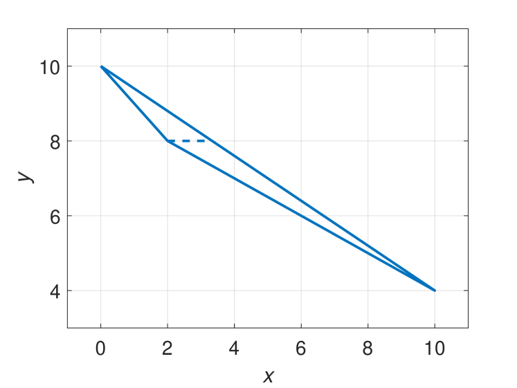
Figure 1: The approximation of the projection of $\tilde{\mathcal{P}}$ via Problem (9).

Clearly, the formulation of Problem (9) is very conservative. It actually requires the homothet of the polytope $\mathbb{B}$ be entirely contained in $\tilde{\mathcal{P}}$. It amounts to each time fixing $\bar{u}=\bar{u}_{0}$, and then measuring the cross section of $\tilde{\mathcal{P}}$. However, for approximating the projection of $\tilde{\mathcal{P}}$, we only need

$$\forall u\in\lambda\mathbb{B}+\mu,\ \exists\bar{u}(u),\mbox{ such that }(u,\bar{u}(u))\in\tilde{\mathcal{P}},$$ (11)

where $\bar{u}$ is a function of $u$, while in Problem (9) $u$ is determined by $\bar{u}$. The relation (11) can be interpreted in the context of the adjustable robust optimization problem [3], where $u$ is the so called non-adjustable variable, and $\bar{u}$ is the adjustable variable. The function $\bar{u}(u)$ is called the decision rule. Solving (9) over all possible choices of $\bar{u}(u)$ is intractable. An efficient way to overcome this is to restrict the choice of $\bar{u}(u)$ to be the affine decision rules,

$$\bar{u}=Wu+V,$$ (12)

where $W\in\mathbb{R}^{\tilde{m}\times m}$, and $V\in\mathbb{R}^{\tilde{m}}$. Using (12) in Problem (9) and by some manipulation, we can obtain

$$\begin{array}[]{ll}\underset{s>0,r,W,V}{\mbox{minimize}}&s\\ \mbox{subject to:}&\mathbb{B}\subset\left\{B\left[\begin{array}[]{c}I\\ W\end{array}\right]u\leq B\left[\begin{array}[]{c}r\\ -V\end{array}\right]+sc\right\}.\end{array}$$ (13)

Using the Farkas’s Lemma, Problem (13) can be solved by the following linear programming

$$(\mbox{APP})\qquad\begin{array}[]{ll}\underset{s>0,G\geq 0,r,W,V}{\mbox{minimize}}&s\\ \mbox{subject to:}&GF=B\left[\begin{array}[]{c}I\\ W\end{array}\right],\\ &GH\leq B\left[\begin{array}[]{c}r\\ -V\end{array}\right]+sc.\end{array}$$

We test the above formulation by computing the approximation of the polytopic projection in Example 1.

Example 2 (Continued).

We solve the Problem (APP) and obtain $r=-0.5$, $s=0.15$. This corresponds to the interval $1/0.15\left(\mathbb{B}+0.5\right)=[0,10]$, which is exactly $\mbox{Proj}_{x}(\tilde{\mathcal{P}})$.

In general, the Problem (APP) gives a suboptimal solution for the approximation of $\mbox{Proj}_{x}(\tilde{\mathcal{P}})$ with respective to $\mathbb{B}$. A possible way to reduce the conservativeness is to employ the quadratic decision rule or other nonlinear decision rules as reported in [3].

IV-B Aggregation of the PEVs’ Flexibility

In this subsection, the polytopic projection approximation developed in the above section will be employed to aggregate the PEVs’ flexibility. We will discuss several issues including the choice of the nominal model $\mathbb{B}$, the preprocessing of the charging constraints, and the strategy for parallel computation. Finally, the explicit formulae for the flexibility model and the corresponding scheduling policy are derived.

IV-B1 Choice of the Nominal Model

Intuitively, one can choose the nominal polytope $\mathbb{B}$ to be of the similar form of (2), and the parameters can be taken as the mean values of the PEV group. More generally, we can define the virtual battery model as follows.

Definition 2.

The set $\mathbb{B}(\phi)$ is called a $m$-horizon discrete time virtual battery with parameters $\phi:=\{\underline{p},\bar{p},\underline{E},\bar{E}\}$, if

$$\mathbb{B}(\phi):=\{u\in\mathbb{R}^{m}:\underline{p}\leq u\leq\bar{p}\mbox{ and }{\bf 1}_{m}^{T}u\in[\underline{E},\bar{E}]\}.$$

$\mathbb{B}(\phi)$ is called a sufficient battery if $\mathbb{B}(\phi)\subset\mathcal{P}$.

Conceptually, the virtual battery model mimics the charging/discharging dynamics of a battery. We can regard $u$ as the power draw of the battery, $\underline{p}$ and $\bar{p}$ as its discharging/charging power limits, and $\bar{E}$ and $\underline{E}$ as the energy capacity limits. Geometrically, it is a polytope in $\mathbb{R}^{m}$ with $2m+2$ facets, which is computationally very efficient when posed as the constraint in various optimization problems.

IV-B2 Preprocessing the Charging Constraints

Note that the original high-dimensional polytope $\tilde{\mathcal{P}}$ defined in (6) contains equality constraints, which is not full dimensional. Therefore, first we have to remove the equalities by substituting the variables. For simplicity, assume that $\bar{E}^{i}>\underline{E}^{i}$. More explicitly, let $u_{t}^{i}$ be the $i^{\mbox{th}}$ PEV’s charging profile at time $t$, $\forall i\in\mathcal{N}$, and $\forall t\in\mathbb{T}$, $u_{t}$ be the generation profile at time $t$. The overall charging constraints of the PEV group can be written as follows

$$\begin{cases}u_{t}=\sum_{i=1}^{N}\mathbbm{1}_{\mathbb{A}^{i}}(t)u_{t}^{i},&\forall t\in\mathbb{T},\\ 0\leq u_{t}^{i}\leq p^{i},&\forall i\in\mathcal{N},\mbox{ and }\forall t\in\mathbb{A}^{i},\\ u_{t}^{i}=0,&\forall i\in\mathcal{N},\mbox{ and }\forall t\in\mathbb{T}\backslash\mathbb{A}^{i},\\ \underline{E}^{i}\leq\sum_{t=a^{i}}^{d^{i}}u_{t}^{i}\leq\bar{E}^{i},&\forall i\in\mathcal{N},\end{cases}$$ (14)

which is a polytope in $\mathbb{R}^{(N+1)m}$, and the coordinate is designated to be $(u,u^{1},u^{2},\cdots,u^{N})$. We first need to eliminate the equality constraints containing $(u^{1},u^{2},\cdots,u^{N})$, i.e., the first line of (14). To standardize the elimination process, define $N_{t}:=\{i\in\mathcal{N}|t\in\mathbb{A}^{i}\}$, which is the index set of the PEVs that can be charged at time $t$. Without loss of generality, assume that $N_{t}\neq\emptyset$, $\forall t\in\mathbb{T}$, and we substitute $u_{t}^{j_{t}}=u_{t}-\sum_{i\in N_{t}\backslash j_{t}}u_{t}^{i}$, $\forall t\in\mathbb{T}$ in (14), where $j_{t}:=\min_{i\in N_{t}}i$ is the first PEV in the set $N_{t}$. Let $S_{i}:=\{t\in\mathbb{A}^{i}:j_{t}=i\}$ be the set of time instants at which the substitution of $u_{t}^{i}$ is made. Further, we remove the coordinate $u_{t}^{i}=0$ and obtain,

$$\begin{cases}0\leq u_{t}-\sum_{i\in N_{t}\backslash\{j_{t}\}}u_{t}^{i}\leq p^{j_{t}},&\forall t\in\mathbb{T},\\ 0\leq u_{t}^{i}\leq p^{i},&\forall t\in\mathbb{T},i\in N_{t}\backslash\{j_{t}\},\\ \underline{E}^{i}\leq\sum_{t\in\mathbb{A}^{i}\backslash S_{i}}u_{t}^{i}\\ +\sum_{t\in S_{i}}\left\{u_{t}-\sum_{i\in N_{t}\backslash j_{t}}u_{t}^{i}\right\}\leq\bar{E}^{i},&\forall i\in\mathcal{N},\end{cases}$$ (15)

where the new coordinate becomes $(u,\tilde{u}),$ with

$$\tilde{u}:=(\tilde{u}^{1},\tilde{u}^{2},\cdots,\tilde{u}^{N})$$ (16)

and $\tilde{u}^{i}=[u_{t}^{i}]_{t\in\mathbb{A}^{i}\backslash S_{i}}$, $i\in\mathcal{N}$. Clearly, $\tilde{u}$ has a dimension $\tilde{m}:=\sum_{i=1}^{N}(d^{i}-a^{i}+1)-m$, and there are a number of $n:=2(N+\sum_{i=1}^{N}(d^{i}-a^{i}+1))$ linear inequalities in (15). We denote it by the matrix form,

$$B\left[\begin{array}[]{c}u\\ \tilde{u}\end{array}\right]\leq c,$$ (17)

where note that $B\in\mathbb{R}^{n\times(m+\tilde{m})}$ is a sparse matrix and has the structure,

$$B=\left[\begin{array}[]{cc}B_{11}&B_{12}\\ 0_{2\tilde{m}\times m}&B_{22}\end{array}\right].$$

IV-B3 Scalability

For a fixed time horizon $m$, both the number of the decision variables and the number of inequality constraints of Problem (APP) increase linearly with $\tilde{m}$. When the number of PEVs to be aggregated is too large, solving Problem (APP) would be intractable. To address the increasing numerical complexity, we propose to divide the PEVs into small groups, and solve Problem (APP) for each group with respect to the same nominal model $\mathbb{B}$. Denoting the solutions of Problem (APP) for the $k^{\mbox{th}}$ group by $(s_{k},r_{k},W_{k},V_{k},G_{k})$, the aggregate flexibility of the $k^{\mbox{th}}$ group is given by $1/s_{k}(\mathbb{B}-r_{k})$. Then the flexibility of the overall PEV group can be calculated directly based on the following lemma.

Lemma 1.

Let $\mathbb{B}$ be a polytope, and $\lambda_{1}$, $\lambda_{2}$ be non-negative scalars. Then $\lambda_{1}\mathbb{B}\oplus\lambda_{2}\mathbb{B}=(\lambda_{1}+\lambda_{2})\mathbb{B}$.

The above result can be easily verified. A more general proof for the convex body can be found in [28, Remark 1.1.1]).

By this “divide and conquer” strategy, the original highly complex optimization problem can be solved very efficiently in a parallel fashion. However, this increases the conservativeness of the approximation, which is a result of the trade-off between the tractability and the optimality.

In case that different nominal models $\mathbb{B}^{k}$ are used for each group, we can perform the aggregation again over the obtained groups. Repeating this after several stages, we can arrive one virtual battery model for the overall PEV group. Even though we have to spread the computation over time in different stages, in practice this process terminates soon since the number of stages is of order $\log_{x}^{N}$ when $x$ PEVs/groups are processed at each run of Problem (APP).

IV-B4 Design of the Sufficient Virtual Battery

Combining the above development, the following explicit formulae for designing the sufficient virtual battery can be derived. The scheduling policy for each individual PEVs can also be obtained. Without loss of generality, these results are stated for the case where only one stage aggregation is executed. The formulae for multi-stage aggregation can be obtained analogously. For convenience, let us denote the solutions of the Problem (APP) by the output of the function $(s_{k},r_{k},W_{k},V_{k},G_{k})=\mbox{APP}(\mathcal{\tilde{P}}^{k},\mathbb{B}),$ where $\mathcal{\tilde{P}}^{k}$ is the high-dimensional polytope associated with the $k^{\mbox{th}}$ group of PEVs, and $\mathbb{B}$ is a given nominal model parameterized by $(\bar{p},\underline{p},\bar{E},\underline{E})$. The proof of the following theorem can be found in the Appendix -B.

Theorem 2.

Suppose $(s_{k},r_{k},W_{k},V_{k},G_{k})=\mbox{APP}(\tilde{\mathcal{P}}^{k},\mathbb{B})$, $\forall k$. Then $\mathbb{B}_{s}=\lambda\mathbb{B}+\mu$ is a sufficient battery parameterized by

$$\bar{u}_{s}= \lambda\bar{p}+\mu,$$

$$\underline{u}_{s}= \lambda\underline{p}+\mu,$$

$$\bar{E}_{s}= \lambda\bar{E}+{\bf 1}_{m}^{T}\mu,$$

$$\underline{E}_{s}= \lambda\underline{E}+{\bf 1}_{m}^{T}\mu,$$

where $\lambda=\sum_{k}\lambda_{k}$, $\mu=\sum_{k}\mu_{k}$ and $\lambda_{k}=\frac{1}{s_{k}}$ , $\mu_{k}=\frac{-r_{k}}{s_{k}}$. Furthermore, $\forall u\in\mathbb{B}_{s},$ the scheduling policy is given by

$$\tilde{u}_{k}=W_{k}\frac{\lambda_{k}}{\lambda}(u-\mu)+\lambda_{k}V_{k},$$ (19)

where $\tilde{u}_{k}=(\tilde{u}_{k}^{1},\tilde{u}_{k}^{2},\cdots,\tilde{u}_{k}^{N_{k}})$ denotes the charging profiles of the number of $N_{k}$ PEVs in the $k^{\mbox{th}}$ group.

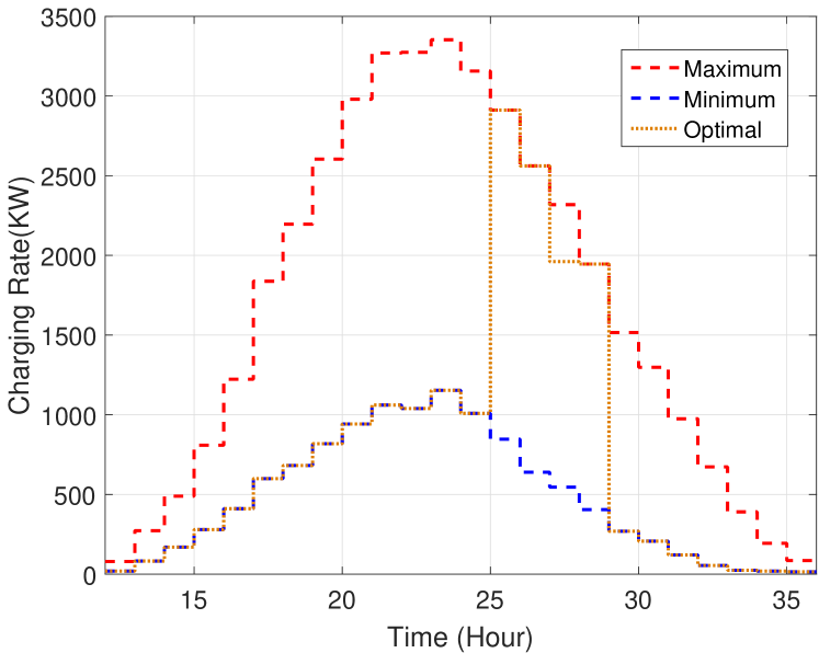
Figure 2: The maximum and the minimum charging rates of the designed virtual battery model.

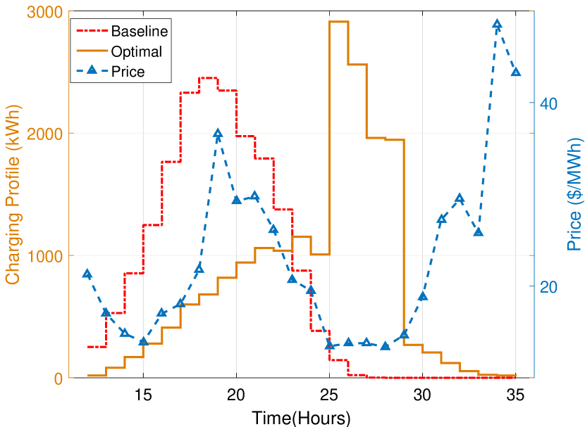
Figure 3: Aggregate charging profile versus the price.

V Simulation

In this section, we consider coordination of a group of 1000 PEVs for energy arbitrage. The considered time horizon is 24 hours, and the price is taken as the Day-Ahead Energy Market locational marginal pricing (LMP) [1]. The parameters of PEVs are randomly generated by their types and the corresponding probability distributions (see [13] for more details). Since most of the PEVs arrive during the afternoon to midnight and leave during the next 12 hours, we choose to simulate from 12:00 noon to the same time on the next day. In addition, we assume a $\pm 5\%$ total charging energy flexibility around the nominal energy requirement. The (APP) problem is solved using the GLPK linear programming solver [2] interfaced with YALMIP [21]. At the first stage, we randomly divide the 1000 PEVs into 100 groups, where each group contains 10 PEVs. The aggregate flexibility approximation is thus solved for 10 PEVs in one group. This number is chosen according to the numerical efficiency of the solver. The parameters of the nominal battery model $\mathbb{B}$ for each group are chosen as the average values of the group. For those groups having the same minimum arrival time and maximum departure time, we take the average values between them and approximate their flexibilities using the same nominal model. For example, by setting the elements in the charging matrix $M$ by their maximum values, the upper charging limits $\bar{p}$ for the nominal battery model are calculated as the column averages of $M$. Since these groups share the same nominal model, their approximated aggregated flexibilities can be calculated very easily based on Lemma 1. In our simulation, after the first stage, the 100 groups are merged into 22 collections which are represented by polytopes of different codimensions. Then we repeat the process in the first stage to approximate the flexibility of these 22 collections, where each time we aggregate 11 collections. Finally a sufficient battery model $\mathbb{B}_{s}$ is obtained for the characterization of the aggregate flexibility of the entire loads group.

The dynamic charging limits of the obtained battery model are illustrated in Fig. 2. The total charging energy bounds are obtained as $\underline{E}=18.35$ MWh and $\bar{E}=19.09$ MWh, which lies in the true aggregate energy consumption interval $l_{E}:=[17.65,19.51]$ MWh. From Fig. 2, we can see that around the midnight (the $24^{\mbox{th}}$ hour), the charging flexibility of the PEVs are the largest in terms of the difference of the charging rate bounds. Denoting the energy price by $\pi$, and the planned energy by $z$, the energy arbitrage problem can be formulated as a linear programming problem as follows,

$$\begin{array}[]{ll}\underset{z}{\mbox{minimize}}&\pi^{T}z\\ \mbox{subject to:}&z\in\mathbb{B}_{s}.\end{array}$$

Clearly, the above optimization problem can be solved much more efficiently than directly optimizing the power profiles subject to the constraints of 1000 PEVs. We plot the obtained power profiles against the price changes in Fig. 3. It can be observed that most of the energy demand are consumed during $1:00\mbox{AM}$ $(25^{\mbox{th}}\mbox{ hour})$ to $4\mbox{AM}$ $(28^{\mbox{th}}\mbox{ hour})$ in the morning, when the prices are at its lowest. The same curve of the planned power is also plotted in Fig. 2 (the dotted line), where note we assume that the time discretization unit is $1$ hour. We see that the planned charging rate lies in the charging bounds of $\mathbb{B}_{s}$, and almost always matches the maximum/minimum bound. Using this charging profile, the total energy being charged to the PEVs is $18.34$ MWh which lies in the interval $l_{E}$. Hence, it is adequate and the charging requirement of individual PEV can be guaranteed by using the scheduling policy (19).

We choose the immediate charging policy as the baseline and use it to compare with the obtained optimal charging profile in Fig. 2. To ensure a fair comparison, we impose an additional constraint that the total energies consumed by both profiles are the same. The total energy cost for the baseline charging profile is $430.8\$$, while the cost for the optimal charging profile is $343.0\$$, which reduces the baseline cost by about $20\%$.

VI Conclusions and Future Work

This paper proposed a novel polytopic projection approximation method for extracting the aggregate flexibility of a group of heterogeneous deferrable loads. The aggregate flexibility of the entire load group could be extracted parallelly and in multiple stages by solving a number of linear programming problems. The scheduling policy for individual load was simultaneously derived from the aggregation process. Finally, a PEV energy arbitrage problem was solved to demonstrate the effectiveness of our approach at characterizing the feasible aggregate power flexibility set, and facilitating finding the optimal power profile.

Our future work includes studying the performances of using other decision rules such as the quadratic decision rule and the nonlinear decision rule, and as compared to the method using Zonotopes. In addition, it is interesting to consider a probabilistic description of the aggregate flexibility as in practice the uncertainty of the loads parameters must be considered to reduce the risk of over-estimating or under-estimating the aggregated flexibility.

-A Farkas’ lemma

For the sake of completeness, we restate the following version of Farkas’s lemma as used in [12], which will be used to derive our algorithm for approximating the polytopic projection. Its proof can be found in [22].

Lemma 2.

(Farkas’ lemma) Suppose that the system of inequalities $Ax\leq b,$ $A\in\mathbb{R}^{m\times n}$ has a solution and that every solution satisfies $Fx\leq d,$ $F\in\mathbb{R}^{k\times n}$. Then there exists $G\in\mathbb{R}^{k\times m}$ , $G\geq 0$, such that $GA=F$ and $Gb\leq d$.

-B Proof of Theorem 2

(1) Sufficient battery: since $(s_{k},r_{k})$ is the solution of the APP problem, we have $\lambda_{k}\mathbb{B}+\mu_{k}\subset\tilde{\mathcal{P}}^{k}$, where $\lambda_{k}=1/s_{k}$ and $\mu_{k}=-r_{k}/s_{k}$. Let

$$\mathbb{B}_{s}:=\biguplus_{k}(\lambda_{k}\mathbb{B}+\mu_{k}),$$

and it can be shown that,

$$\mathbb{B}_{s} =\biguplus_{k}\lambda_{k}\mathbb{B}+\mu$$

$$=\lambda\mathbb{B}+\mu,$$

where $\lambda=\sum_{k}\lambda_{k},\mu=\sum_{k}\mu_{k}$, and the last equality is derived by using Lemma 1. Since

$$\biguplus_{k}(\lambda_{k}\mathbb{B}+\mu_{k})\subset\biguplus_{k}\tilde{\mathcal{P}}^{k}=\tilde{\mathcal{P}},$$

we see $\mathbb{B}_{s}$ is sufficient. Now suppose $u\in\mathbb{B}_{s}$, then $(u-\mu)/\lambda\in\mathbb{B}$. Denoting $\mathbb{B}$ by its facet representation, we have $\mathbb{B}=\{Fu\leq H\}$, where

$$F= [I_{m},I_{m},{\bf 1}_{m},{\bf 1}_{m}]^{T},$$

$$H= (\bar{u},-\underline{u},\bar{E},-\underline{E}),$$

and then parameters of $\mathbb{B}_{s}$ can be obtained from

$$Fu\leq\lambda H+F\mu.$$

(2) Scheduling policy: given a generation profile $u$ in $\mathbb{B}_{s}$, we can decompose it into the individual admissible power profile $\tilde{u}$ through two steps. First, we decompose it into the generation profiles for each groups: $\forall u\in\mathbb{B}_{s}$, by part (1) we know

$$\frac{1}{\lambda}(u-\mu)\in\mathbb{B},$$

and further more

$$\frac{\lambda_{k}}{\lambda}(u-\mu)+\mu_{k}\in\tilde{\mathcal{P}}^{k}.$$

Denoting the generation profile for the $k^{\mbox{th}}$ group by

$$z_{k}:=\frac{\lambda_{k}}{\lambda}(u-\mu)+\mu_{k},$$

and hence, $z_{k}\in\lambda_{k}\mathbb{B}+\mu_{k}$ which is the aggregate flexibility extracted from the $k^{\mbox{th}}$ group. It can be further decomposed into each PEVs in the $k^{\mbox{th}}$ group. Now we need to use the linear decision rule in (12). Note that the decision rule (12) is applied in (13) which actually maps from $\mathbb{B}$ to $s_{k}\tilde{\mathcal{P}}^{k}+(r_{k},\mathbf{0})$, while the decomposition mapping we need is actually from $\lambda_{k}\mathbb{B}+\mu_{k}$ to $\tilde{\mathcal{P}}^{k}$. The mappings between these four polytopes form a commutative diagram (see below). Observe that the linear ratio of the decomposition mapping does not change, and only the translate vector needs to be calculated. Therefore, assume that the decomposition takes the form

$$\tilde{u}_{k}=W_{k}z_{k}+U,$$

where $U$ is the translate vector to be determined.

From the above commutative diagram, we must have $\forall z_{k}\in\lambda_{k}\mathbb{B}+\mu_{k}$,

$$s_{k}\left(W_{k}z_{k}+U\right)+\mathbf{0}=W_{k}\left(s_{k}z_{k}+r_{k}\right)+V_{k}.$$

Solve the above equality and we will have

$$U=\lambda_{k}V_{k}-W_{k}\mu_{k},$$

and the overall scheduling policy (19) follows from the composition of $z_{k}$ and $\tilde{u}_{k}$. ∎

References

- [1] “PJM Daily Day-Ahead locational marginal pricing.” [Online]. Available: http://www.pjm.com/markets-and-operations/energy/day-ahead/lmpda.aspx
- [2] “GLPK (GNU linear programming kit),” 2006. [Online]. Available: http://www.gnu.org/software/glpk
- [3] A. Ben-Tal, A. Goryashko, E. Guslitzer, and A. Nemirovski, “Adjustable robust solutions of uncertain linear programs,” Mathematical Programming, vol. 99, no. 2, pp. 351–376, 2003.
- [4] A. Ben-Tal, L. E. Ghaoui, and A. Nemirovski, Robust Optimization. Princeton University Press, 2009.
- [5] J. Bhatt, V. Shah, and O. Jani, “An instrumentation engineer’s review on smart grid: critical applications and parameters,” Renewable and Sustainable Energy Reviews, vol. 40, pp. 1217–1239, Dec. 2014.
- [6] R. A. Brualdi and G. Dahl, “Matrices of zeros and ones with given line sums and a zero block,” Linear Algebra and its Applications, vol. 371, pp. 191–207, Sept. 2003.
- [7] D. S. Callaway, “Tapping the energy storage potential in electric loads to deliver load following and regulation with application to wind energy,” Energy Conversion and Management, vol. 50, no. 5, pp. 1389 –1400, May 2009.
- [8] D. S. Callaway and I. A. Hiskens, “Achieving controllability of electric loads,” Proceedings of the IEEE, vol. 99, no. 1, pp. 184 – 199, 2011.
- [9] W. Chen, L. Qiu, and P. Varaiya, “Duration-deadline jointly differentiated energy services,” in the 54th IEEE Conference on Decision and Control, Dec. 2015, pp. 7220–7225.
- [10] W. Chen, Y. Mo, L. Qiu, and P. Varaiya, “A structure tensor condition for (0,1)-matrices with given row and column sums and certain fixed zeros,” 2015, in preprint.
- [11] W. Y. Chen, “Integral matrices with given row and column sums,” Journal of Combinatorial Theory, Series A, vol. 61, no. 2, pp. 153–172, 1992.
- [12] B. Eaves and R. Freund, “Optimal scaling of balls and polyhedra,” Mathematical Programming, vol. 23, no. 1, pp. 138–147, 1982.
- [13] D. Guo, W. Zhang, G. Yan, Z. Lin, and M. Fu, “Decentralized control of aggregated loads for demand response,” in American Control Conference (ACC), June 2013, pp. 6601–6606.
- [14] H. Hao and W. Chen, “Characterizing flexibility of an aggregation of deferrable loads,” in the 53rd IEEE Annual Conference on Decision and Control, Dec. 2014, pp. 4059–4064.
- [15] H. Hao, B. Sanandaji, K. Poolla, and T. Vincent, “Aggregate flexibility of thermostatically controlled loads,” IEEE Transactions on Power Systems, vol. 30, no. 1, pp. 189–198, Jan. 2015.
- [16] M. Henk, J. Richter-Gebert, and G. M. Ziegler, “Basic properties of convex polytopes,” in Handbook of Discrete and Computational Geometry, J. E. Goodman and J. O’Rourke, Eds. Boca Raton, FL, USA: CRC Press, Inc., 1997, ch. 15, pp. 243–270.
- [17] D. Hershkowitz, A. J. Hoffman, and H. Schneider, “On the existence of sequences and matrices with prescribed partial sums of elements,” Linear Algebra and its Applications, vol. 265, pp. 71–92, Nov. 1997.
- [18] M. Kamgarpour, C. Ellen, S. Soudjani, S. Gerwinn, J. Mathieu, N. Mullner, A. Abate, D. Callaway, M. Franzle, and J. Lygeros, “Modeling options for demand side participation of thermostatically controlled loads,” in Bulk Power System Dynamics and Control - IX Optimization, Security and Control of the Emerging Power Grid, IREP Symposium, Aug. 2013, pp. 1–15.
- [19] S. Koch, J. Mathieu, and D. Callaway, “Modeling and control of aggregated heterogeneous thermostatically controlled loads for ancillary services,” in 17th Power system Computation Conference, Stockholm, Sweden, August 2011.
- [20] J. Liu, S. Li, W. Zhang, J. L. Mathieu, and G. Rizzoni, “Planning and control of electric vehicles using dynamic energy capacity models,” in the 52nd IEEE Annual Conference on Decision and Control, Dec. 2013, pp. 379–384.
- [21] J. Löfberg, “ YALMIP : A toolbox for modeling and optimization in MATLAB,” in Proceedings of the CACSD Conference, Taipei, Taiwan, 2004. [Online]. Available: http://users.isy.liu.se/johanl/yalmip
- [22] O. Mangasarian, “Set containment characterization,” Journal of Global Optimization, vol. 24, no. 4, pp. 473–480, 2002.
- [23] A. W. Marshall, I. Olkin, and B. C. Arnold, Inequalities: Theory of Majorization and Its Applications, 2nd ed. Springer, 2010.
- [24] J. Mathieu, M. Kamgarpour, J. Lygeros, and D. Callaway, “Energy arbitrage with thermostatically controlled loads,” in European Control Conference, July 2013, pp. 2519–2526.
- [25] F. L. Müller, O. Sundström, J. Szabó, and J. Lygeros, “Aggregation of energetic flexibility using zonotopes,” in the 54th IEEE Conference on Decision and Control, Dec. 2015, pp. 6564–6569.
- [26] A. Nayyar, J. Taylor, A. Subramanian, K. Poolla, and P. Varaiya, “Aggregate flexibility of a collection of loads,” in the 52nd IEEE Annual Conference on Decision and Control, Dec. 2013, pp. 5600–5607.
- [27] N. Ruiz, I. Cobelo, and J. Oyarzabal, “A direct load control model for virtual power plant management,” IEEE Transactions on Power Systems, vol. 24, no. 2, pp. 959–966, May 2009.
- [28] R. Schneider, Convex Bodies: The Brunn-Minkowski Theory. Cambridge University Press, 1993.
- [29] H. Tiwary, “On the hardness of computing intersection, union and Minkowski sum of polytopes,” Discrete & Computational Geometry, vol. 40, no. 3, pp. 469–479, 2008.
- [30] C. Weibel, “Minkowski sums of polytopes: Combinatorics and computation,” Ph.D. dissertation, École Polytechnique Fédérale De Lausanne, 2007.
- [31] L. Zhao and W. Zhang, “A unified stochastic hybrid system approach to aggregated load modeling for demand response,” in the 54th IEEE Conference on Decision and Control, Dec. 2015, pp. 6668–6673.
- [32] ——, “A geometric approach to virtual battery modeling of thermostatically controlled loads,” in American Control Conference, July 6-8, Boston, MA, USA, 2016, pp. 1452-1457.
- [33] J. Zhen and D. den Hertog, “Computing the maximum volume inscribed ellipsoid of a polytopic projection,” CentER Discussion Paper Series No. 2015-004, Jan. 2015.