On Optimal Exact Simulation of Max-Stable and Related Random Fields on a Compact Set

Abstract.

We consider the random field

$$M(t)=\sup_{n\geq 1}\big{\{}-\log A_{n}+X_{n}(t)\big{\}}\,,\qquad t\in T\,,$$

for a set $T\subset\mathbb{R}^{m}$, where $(X_{n})$ is an iid sequence of centered Gaussian random fields on $T$ and $0<A_{1}<A_{2}<\cdots$ are the arrivals of a general renewal process on $(0,\infty)$, independent of $(X_{n})$. In particular, a large class of max-stable random fields with Gumbel marginals have such a representation. Assume that one needs $c\left(d\right)=c(\{t_{1},\ldots,t_{d}\})$ function evaluations to sample $X_{n}$ at $d$ locations $t_{1},\ldots,t_{d}\in T$. We provide an algorithm which, for any $\epsilon>0$, samples $M(t_{1}),\ldots,M(t_{d})$ with complexity $o(c(d)\,d^{\epsilon})$ as measured in the $L_{p}$ norm sense for any $p\geq 1$. Moreover, if $X_{n}$ has an a.s. converging series representation, then $M$ can be a.s. approximated with error $\delta$ uniformly over $T$ and with complexity $O(1/(\delta\log(1/\delta))^{1/\alpha})$, where $\alpha$ relates to the Hölder continuity exponent of the process $X_{n}$ (so, if $X_{n}$ is Brownian motion, $\alpha=1/2$).

1. Introduction

Let $X$ be a centered Gaussian random field on a set $T\subseteq\mathbb{R}^{m}$, $m\geq 1$ and consider a sequence $\left(X_{n}\right)$ of independent and identically distributed  copies of $X$. In addition, let $\left(A_{n}\right)$ be a renewal sequence independent of $\left(X_{n}\right)$. Under mild regularity conditions on the $X$, we will provide an efficient Monte-Carlo algorithm for sampling the field

(1.1) $$M(t)=\sup_{n\geq 1}\big{\{}-\log A_{n}+X_{n}(t)+\mu(t)\big{\}},\qquad t\in T\,,$$

where $\mu:T\longrightarrow\mathbb{R}$ is a bounded function.

We will design and analyze an algorithm for the exact simulation of

$$M(t_{1}),\ldots,M(t_{d})\quad\mbox{for any choice of distinct locations $t_{1},...,t_{d}\in T$,}$$

and we will show that, in some sense, this algorithm is asymptotically optimal as $d\rightarrow\infty$.

The algorithm proposed here shaves off a factor of order (nearly) $d$ from the running time of any of the existing exact sampling procedures. In particular, we will show that, under mild boundedness assumptions on $X$, it is as hard to sample $(M(t_{i}))_{i=1,\ldots,d}$ as it is to sample $(X(t_{i}))_{i=1,\ldots,d}$. Therefore, at least from a simulation point of view, it is not more difficult to work with $M$ than with $X$. More precisely, if it takes $O(c(d))$ units of computing time to sample $X$ at $d$ distinct locations $t_{1},\ldots,t_{d}\in T$, then, for any given $\epsilon>0$, it takes $o(c(d)\,d^{\epsilon})$ units to sample $M$ at the same locations; see Theorem 2.2 for a precise formulation.

We illustrate this result by considering fractional Brownian motion $X$ on $T=[0,1]$. Using the circulant-embedding method (see [3], Section XI.3), we have $c(d)=O(d\log d)$ provided we sample at the dyadic points $t_{i}=i/2^{-m}$ for $i=1,\ldots,2^{m}=d$ (which we call dyadic points at level $d$). In the case of Brownian motion, one even has $c(d)=O(d)$, corresponding to the simulation of $d$ independent Gaussian random variables. Thus, in the case of fractional Brownian motion on $[0,1]$ we provide an algorithm for sampling $M$ at the dyadic points at level $d$ in [0,1] with complexity $o(d^{1+\epsilon})$ for any $\epsilon>0$; see [3, Sec. XI.6].

Moreover, if $X$ has a series representation a.s. converging uniformly on $T$ (such as the Lévy-Ciesielski representation for Brownian motion, see [28, Sec. 3.1]), we also propose an approximate simulation procedure for $M$ with a user-defined (deterministic) bound on the error which holds with probability one uniformly throughout $T$. More precisely, for any $\delta>0$, the procedure that we present outputs an approximation $M_{\delta}$ to $M$ such that

(1.2) $$\sup_{t\in T}|M(t)-M_{\delta}(t)|\leq\delta\qquad\mathrm{a.s.}$$

The results concerning (1.2) are reported in Theorem 7.4. The method of designing a family $(M_{\delta})_{\delta>0}$ such that (1.2) holds is known as Tolerance Enforced Simulation (TES) or $\delta$-strong simulation; see [9] and [27] for details. Note that a TES algorithm enforces a strong (almost sure) guarantee without knowledge of any specific set of sampling locations. This is a feature which distinguishes TES from more traditional algorithms in the broad literature on simulation of random fields and processes.

As will be explained later, the evaluation of $M_{\delta}(t)$ for fixed $t$ takes $O(1)$ units of computing time while the construction of the process $M_{\delta}$ will often take $O(1/(\delta\log(1/\delta))^{2})$ units. The latter result holds under assumptions on the convergence of the series representation of $X$ which, in particular, are satisfied for Brownian motion $X$. In the latter case, the proposed procedure achieves a complexity of order $O(d)$ for the exact sampling of $M$ on the dyadic points at level $d$ (because the series truncated at level $d$ is exact on the dyadic points at level $d$). Therefore, the exact sampling procedure based on Theorem 7.4 applied to the dyadic points at level $d$ is optimal because it takes $O(d)$ computational cost to sample $X$ at $d$ dyadic points. Moreover, the convergence rate of the TES algorithm is also optimal in the Brownian case. In order to obtain a uniform error of order $O(\delta)$, one requires to discretize Brownian motion using a grid of size $O(1/(\delta\log(1/\delta))^{2})$; see [5].

Our results are mainly motivated by application to the simulation of max-stable random fields. Indeed, if $(A_{i})$ is the arrival sequence of a unit rate Poisson process on $(0,\infty)$, $M$ is a max-stable process in the sense of de Haan [21]. This means, in particular, that the distribution of $M(t)$ for any fixed $t\in T$ has a Gumbel distribution which is one of the max-stable distributions. The latter class of distributions consists of the non-degenerate limit distributions for the suitably centered and scaled partial maxima of an iid sequence; see for example [19]. The non-Gumbel max-stable processes with Fréchet or Weibull marginals are obtained from the representation (1.1) by suitable monotone transformations. We also mention that de Haan [21] already proved that max-stable processes with Gumbel marginals have representation (1.1), where $X$ may have a rather general dependence structure not restricted to Gaussian $X$. However, the case of Gaussian $X$ has attracted major attention. The case of Brownian $X$ was treated in [15]; it is known as the Brown-Resnick process. In the paper [23], the case of a general Gaussian process $X$ with stationary increments was treated, including the case of a Gaussian process $X$ defined on a multidimensional set $T$ often referred to as Smith model. It is used in environmental applications for modeling storm profiles; see for example [30]. General characterizations, including spectral representations and further properties, have been obtained as well; for example, see [29] and [23]. However, the explicit joint distribution of the max-stable process is in general not tractable. Because max-stable processes are generated as weak limits of maxima of iid random fields, max-stable models are particularly suited for modeling extremal events in spatio-temporal contexts. These include a wide range of applications of environmental type, for example, extreme rainfall [20] and extreme temperature [32].

Recently, several exact sampling procedures for $M$ have been proposed and studied in the literature. In [17], an elegant and easy-to-implement procedure was proposed for the case in which $X$ has stationary increments. Such a procedure has a computational complexity at least of order $O(c(d)\,d)$; see Proposition 4 in [18]. So, for example, if $X$ is fractional Brownian motion, the procedure takes at least $O(d^{2}\log d)$ units of computing time to produce $d$ dyadic points of $M$ in $[0,1]$.

Another exact simulation method for $M$ was recently proposed in [18]. It also has complexity $O(c(d)\,d)$ (see Proposition 4 in [18]), thus the procedure in [18] takes $O(d^{2}$) for fractional Brownian motion (neglecting the contribution of logarithmic factors). This method is based on the idea of simulating the extremal functions. It is completely different from the approach taken here. Additional work concentrates on max-stable processes which satisfy special characteristics. For example, [29] proposed an exact simulation algorithm for the moving maxima model under suitable uniformity conditions.

Another recent development is [26], where the authors discuss an exact sampling algorithm for max-stable fields using the so-called normalized spectral representation. If the normalized spectral functions can be sampled with cost $c_{\text{\tiny{NS}}}(d)$, then the algorithm in [26] samples the max-stable field exactly with complexity $O(c_{\text{\tiny{NS}}}(d))$. However, for Gaussian-based max-stable fields, it is an open problem to devise exact sampling algorithms for the normalized spectral function, and it is unclear how $c_{\text{\tiny{NS}}}(d)$ compares with the complexity $c(d)$ of sampling $X$.

An important difference between our method and those in [17] and [18] is the following: Both [17] and [18] take advantage of representations or structures which allow to truncate the infinite max-convolution in (1.1) while preserving the simple Gaussian structure of the number of terms in the truncation. Because the simple structure of these terms is preserved, the number of terms in the truncation increases at least linearly in $d$. In contrast, we are able to truncate the number of terms in the infinite max-convolution uniformly in $d$. While the terms in the truncation have a slightly more complex structure (they are no longer iid Gaussian), they are still quite tractable from a simulation standpoint.

This paper is organized as follows: In Section 2 we present our main result and in Section 3 we discuss our general strategy, based on milestone events or record-breakers. The record-breaking strategy is illustrated in Section 4 in the setting of random walks, which is needed in our context due to the presence of $(A_{n})$ in $M$. Then we apply the record-breaking strategy to the setting of maxima of Gaussian random vectors with focus on Section 5: This section describes the main algorithmic developments of the paper. A complexity analysis is performed in Section 6. We introduce and analyze a TES algorithm in Section 7. Finally, in Section 8, we conclude our paper with a series of empirical comparison results.

2. Main Result

This section provides a formal statement of the main result and its underlying assumptions. We assume that $(A_{n})_{n\geq 0}$ is a renewal sequence, as mentioned in the Introduction. In particular, $A_{0}=0$, and $A_{n}=\tau_{1}+\cdots+\tau_{n}$, $n\geq 1$, where $\left(\tau_{i}\right)$ is an iid sequence of positive random variables, independent of $(X_{n})$.

We introduce the following technical assumptions applicable to $\left(A_{n}\right)$:

1. For any $\gamma<\mathbb{E}\tau_{1}$, there exists some $\theta_{\gamma}>0$ such that $\mathbb{E}[\exp(\theta_{\gamma}(\gamma-\tau_{1}))]=1$.

2. It is possible to sample step sizes under the nominal probability measure as well as under the exponentially tilted distribution

   $$\mathbb{E}\big{[}\exp(\theta_{\gamma}\,(\gamma-\tau_{1}))\mathbf{1}(\tau_{1}\in dt)\big{]}.$$

We also introduce the following assumptions on the Gaussian field $\left(X(t)\right)_{t\in T}$.

1. $\mathbb{E}[X(t)]=0$.

2. $\mathbb{E}[\exp\left(p\sup_{t\in T}X(t)\right)]<\infty$ for any $p\geq 1$.

Remark 2.1.

By Borell’s inequality [1, Thm. 2.1.1], if $T$ is bounded, a sufficient condition for B2) is

$$\mathrm{Var}(X(s)-X(t))\leq c|s-t|^{\beta}$$

for any $s,t\in T$ and some $c>0$, $\beta>0$. Define $\sigma^{2}(t)=\mathrm{Var}\left(X(t)\right)$. Then, under B1) and B2),

$$\sup_{t\in T}\sigma^{2}(t)=\sup_{t\in T}\mathbb{E}[X(t)^{2}]\leq\mathbb{E}\left[\sup_{t\in T}X(t)^{2}\right]<\infty.$$

We also assume that sampling $(X(t_{i}))_{i=1,\ldots,d}$ costs $c(\{t_{1},\ldots,t_{d}\})\geq d$ units of operations. In this paper, a single operation can be any single arithmetic operation, generating a uniform random variable, calculating a Gaussian cumulative probability function, comparing any two numbers, or retrieving a Gaussian quantile value. For simplicity in the notation, we shall simply write $c\left(d\right)=c(\{t_{1},\ldots,t_{d}\})$. The locations $t_{1},...,t_{d}$ will be assumed given throughout our development.

The following is our performance guarantee for our final algorithm, Algorithm M, presented in Section 6. A crucial part of the theorem is that the points $t_{1},\ldots,t_{d}$ for any $d\geq 1$ lie in a fixed set $T$.

Theorem 2.2.

Assume the conditions A1), A2), and B1), B2). Then Algorithm M outputs $M(t_{1}),\ldots,M(t_{d})$ without any bias, and the total number $R$ of operations in the execution of this algorithm satisfies $\mathbb{E}[R^{p}]=o(d^{\epsilon}c(d)^{p})$ for any $p\geq 1$ and $\epsilon>0$.

3. Building Blocks For Our Algorithm

This section serves as a roadmap for the algorithmic elements behind our approach. We start with a few definitions:

$$\overline{X}_{n}=\max_{i=1,\ldots,d}X_{n}(t_{i}),\qquad\underline{X}_{n}=\min_{i=1,\ldots,d}X_{n}(t_{i}).$$

We shall use $\overline{X}$ and $\underline{X}$ to denote generic copies of $\overline{X}_{n}$ and $\underline{X}_{n}$, respectively. We also set $\overline{\mu}=\max_{i=1,\ldots,n}\mu(t_{i})$ and $\underline{\mu}=\min_{i=1,\ldots,n}\mu(t_{i})$.

Our algorithm relies on three random times which are finite a.s. They depend on parameters $a\in(0,1]$, $C\in\mathbb{R}$, $0<\gamma<{\mathbb{E}}[A_{1}]$ to be chosen later.

1. $N_{X}=N_{X}(a,C)$: for all $n>N_{X}$,

   $$\overline{X}_{n}\leq a\log n+C.$$

   A straightforward Borel-Cantelli argument shows that $N_{X}$ is finite.

2. $N_{A}=N_{A}(\gamma)$: for all $n>N_{A}$,

   (3.1) $$A_{n}\geq\gamma n.$$

3. $N_{a}=N_{a}(\gamma,a,C)$: for all $n>N_{a}$,

   (3.2) $$n\gamma\geq A_{1}\,n^{a}\exp(C-\underline{X}_{1}).$$

Applying the defining properties of these random times, we find that for $n>N:=\max(N_{A},N_{X},N_{a})$ and any $t\in\{t_{1},\ldots,t_{d}\}$,

$$-\log A_{n}+X_{n}(t) \leq -\log A_{n}+\overline{X}_{n}$$

$$\leq -\log A_{n}+a\log n+C$$

$$\leq -\log(n\gamma)+a\log n+C$$

$$\leq -\log A_{1}+\underline{X}_{1}$$

$$\leq -\log A_{1}+X_{1}(t).$$

We conclude that, for $t\in\{t_{1},\ldots,t_{d}\}$,

(3.3) $$\sup_{n\geq 1}\left\{-\log A_{n}+X_{n}(t)+\mu(t)\right\}=\max_{1\leq n\leq N}\left\{-\log A_{n}+X_{n}(t)+\mu(t)\right\},$$

and thus we can sample $M(t_{1}),\ldots,M(t_{d})$ with computational complexity $Nc(d)$ plus the overhead to identify $N_{A}$ and $N_{X}$.

From an algorithmic point of view, the key is the simulation of the random variables $N_{X}$, $N_{A}$, and $N_{a}$. If we know how to simulate these quantities, relation (3.3) indicates that we must be able to simulate the sequences $(A_{n})$ and $(X_{n})$ up to and jointly with $N$ which heavily depends on both sequences.

Remark 3.1.

Assumptions A1) and A2) can be removed without loss of generality. To see this, we first observe that for any $r>0$, $\tau_{i}(r)=\min\left(\tau_{i},r\right)\leq\tau_{i}$ and, therefore,

$$A_{n}(r)=\tau_{1}(r)+\cdots+\tau_{n}(r)\leq A_{n}.$$

Moreover, we can select $r>0$ so that $\gamma<\mathbb{E}\left[\tau_{i}(r)\right]<\mathbb{E}[\tau_{i}]$. Hence we can use $\left(A_{n}(r)\right)_{n\geq 1}$ to find $N_{A}$ satisfying

$$A_{n}>A_{n}(r)>\gamma\,n.$$

Because $0\leq\tau_{n}(r)\leq r$, the moment generating function of $\tau_{n}(r)$ exists on the whole real line. By convexity, one can always choose $\theta_{\gamma}$ which satisfies $\mathbb{E}[\exp(\theta_{\gamma}(\gamma-\tau_{1}(r)))]=1$, as long as $\mathrm{Var}\left(\tau_{i}(r)\right)>0$ (i.e. if $\tau_{i}>0$ is non-deterministic, by choosing $r>0$ large enough). If $\tau_{i}$ is deterministic, the strategy can be implemented directly, that is, we can simply select $N_{A}$ deterministic. Once we find $N_{A}$, we can recover $(A_{n})_{n\leq N_{A}}$ from $(A_{n}(r))_{n\leq N_{A}}$ by replacing $\tau_{n}(r)$ with an independent sample of $\tau_{n}$ given $\tau_{n}\geq r$, for any $n\leq N_{A}$ such that $\tau_{n}(r)=r$, and keeping $\tau_{n}(r)$ if it is less than $r$.

Given our previous discussion, we might concentrate on how to sample from an exponentially tilted distribution of a random variable with compact support, which may require evaluating the moment generating function in closed form. Sampling from an exponentially tilted distribution is straightforward for random variables with finite support. So, the strategy can be implemented for $\left\lfloor\tau_{i}\left(r\right)\Delta\right\rfloor/\Delta<\tau_{i}\left(r\right)$, where $\left\lfloor\cdot\right\rfloor$ is the round-down operator, picking $\Delta>0$ sufficiently small so that $\mathbb{E}\left[\left\lfloor\tau_{i}\left(r\right)\Delta\right\rfloor/\Delta\right]>\gamma$. Once $\left\lfloor\tau_{i}\left(r\right)\Delta\right\rfloor$ is sampled we can easily simulate $\tau_{i}\left(r\right)$ using acceptance/rejection. The details of this idea are explained in [13].

4. Sampling a Random Walk up to a Last Passage Time

In this section, we discuss the simulation of the random time $N_{A}$ jointly with the sequence $(A_{n})_{n\geq 0}$. We lead this discussion in the context of a general random walk $(S_{n})_{n\geq 0}$ starting from the origin with negative drift. It is eventually negative almost surely. We review an algorithm from [14] for finding a random time $N_{S}$ such that $S_{n}<0$ for all $n>N_{S}$. Our aim is to develop a sampling algorithm for $(S_{1},\ldots,S_{N_{S}+\ell})$ for any fixed $\ell\geq 0$. Our discussion here provides a simpler version of the algorithm in [14] and allows us to provide a self-contained development of the whole procedure for sampling $M\left(t_{1}\right),\ldots,M\left(t_{d}\right)$.

The algorithm is based on alternately sampling upcrossings and downcrossings of the level $0$. We write $\xi_{0}^{+}=0$ and, for $i\geq 1$, we recursively define

$$\xi_{i}^{-}=\begin{cases}\inf\{n\geq\xi_{i-1}^{+}:S_{n}<0\}&\text{if }\xi_{i-1}^{+}<\infty\\ \infty&\text{otherwise}\end{cases}$$

together with

$$\xi_{i}^{+}=\begin{cases}\inf\{n\geq\xi_{i}^{-}:S_{n}\geq 0\}&\text{if }\xi_{i}^{-}<\infty\\ \infty&\text{otherwise}.\end{cases}$$

As usual, in these definitions the infimum of an empty set should be interpreted as $\infty$. Writing

$$N_{S}=\sup\{\xi_{n}^{-}:\xi_{n}^{-}<\infty\},$$

and keeping in mind that $(S_{n})$ starts as zero and has negative drift, we have by construction $0\leq N_{S}<\infty$ almost surely, and for $n>N_{S}$, $S_{n}\leq 0$. The random variable $N_{S}-1$ is an upward last passage time:

$$N_{S}-1=\sup\{n\geq 0:S_{n}\geq 0\}.$$

We write $\mathbb{P}_{x}$ for the distribution of the random walk starting from $x\in\mathbb{R}$, so that $\mathbb{P}=\mathbb{P}_{0}$. We assume the existence of Cramér’s root, $\theta>0$, satisfying $\mathbb{E}[\exp(\theta S_{1})]=1$. Also assume that we can sample a random walk starting from $x$ under $\mathbb{P}_{x}^{\theta}$, which is defined with respect to $\mathbb{P}_{x}$ through an exponential change of measure: on the $\sigma$-field generated by $S_{1},\ldots,S_{n}$ we have

$$\frac{d\mathbb{P}_{x}}{d\mathbb{P}_{x}^{\theta}}=\exp(-\theta(S_{n}-x)).$$

Under $\mathbb{P}_{x}^{\theta}$, the random walk $(S_{n})$ has positive drift.

The rest of this section is organized as follows:

• In Section 4.1 we discuss sampling of downcrossing and upcrossing segments of the random walk.

• In Section 4.2 we explain how to sample beyond $N_{S}$.

• In Section 4.3 we presents our full algorithm for sampling $(S_{1},\ldots,S_{N_{S}+\ell})$.

4.1. Downcrossings and upcrossings

To introduce the algorithm, we first need the following definitions:

$$\tau^{-}=\inf\{n\geq 0:S_{n}<0\},\quad\quad\tau^{+}=\inf\{n\geq 0:S_{n}\geq 0\}.$$

For $x\geq 0$, it is immediate that we can sample a downcrossing segment $S_{1},\ldots,S_{\tau^{-}}$ under $\mathbb{P}_{x}$ due to the negative drift, and we record this for later use in a pseudocode function. Throughout this paper, ‘sample’ in pseudocode stands for ‘sample independently of anything that has been sampled already.’

Function SampleDowncrossing($x$): Samples $(S_{1},\ldots,S_{\tau^{-}})$ under $\mathbb{P}_{x}$ for $x\geq 0$

Step 1: Return sample $(S_{1},\ldots,S_{\tau^{-}})$ under $\mathbb{P}_{x}$.

Step 2: EndFunction

Sampling an upcrossing segment is much more challenging because it is possible that $\tau^{+}=\infty$, so an algorithm needs to be able to detect this event within a finite amount of computing resources. For this reason, we understand sampling an upcrossing segment under $\mathbb{P}_{x}$ for $x<0$ to mean that an algorithm outputs $(S_{1},\ldots,S_{\tau^{+}})$ if $\tau^{+}<\infty$, and otherwise it outputs ‘degenerate.’

Our algorithm is based on importance sampling and exponential tilting, techniques that are widely used for rare event simulation [3, p. 164]. Under Assumption A1), it is well-known that $\mathbb{E}_{x}^{\theta}[\tau^{+}]<\infty$; for instance, see [2, p. 231, Cor. 4.4]. In particular, the expected time to simulate $(S_{1},\ldots,S_{\tau^{+}})$ is finite under $\mathbb{P}_{x}^{\theta}$ for any $x<0$.

The following proposition is the key to our algorithm.

Proposition 4.1.

Let $x<0$. Suppose there exists some $\theta>0$ with $\mathbb{E}[\exp(\theta S_{1})]=1$. With $U$ being a standard uniform random variable independent of $(S_{n})$ under $\mathbb{P}_{x}^{\theta}$, we have the following:

1. The law of $\mathbf{1}(\tau^{+}<\infty)$ under $\mathbb{P}_{x}$ equals the law of $\mathbf{1}(U\leq\exp(-\theta(S_{\tau^{+}}-x)))$ under $\mathbb{P}^{\theta}_{x}$.

2. The law of $\tau^{+}$ given $\tau^{+}<\infty$ under $\mathbb{P}_{x}$ equals the law of $\tau^{+}$ given $U\leq\exp(-\theta(S_{\tau^{+}}-x))$ under $\mathbb{P}_{x}^{\theta}$.

3. For any $k\geq 1$, the law of $(S_{1},...,S_{k})$ given $\tau^{+}=k$ under $\mathbb{P}_{x}$ equals the law of $(S_{1},\ldots,S_{k})$ given $U\leq\exp(-\theta(S_{\tau^{+}}-x))$ and $\tau^{+}=k$ under $\mathbb{P}_{x}^{\theta}$.

Proof.

For any integer $k\geq 1$ and Borel sets $B_{1},B_{2},\ldots,B_{k}$, we have

$$\mathbb{P}_{x}\left(S_{1}\in B_{1},\ldots,S_{k}\in B_{k},\tau^{+}=k\right)$$

$$= \mathbb{E}_{x}^{\theta}\big{[}\exp(-\theta\,(S_{k}-x))\mathbf{1}(S_{1}\in B_{1},\ldots,S_{k}\in B_{k},\tau^{+}=k)\big{]}$$

$$= \mathbb{E}_{x}^{\theta}\big{[}\mathbf{1}(U\leq\exp(-\theta\,(S_{\tau^{+}}-x)))\,\mathbf{1}(S_{1}\in B_{1},\ldots,S_{k}\in B_{k},\tau^{+}=k)\big{]}.$$

All claims are elementary consequences of this identity, upon noting that $\tau^{+}<\infty$ under $\mathbb{P}_{x}^{\theta}$. ∎

This proposition immediately yields the following algorithm.

Function SampleUpcrossing($x$): Samples $(S_{1},\ldots,S_{\tau^{+}})$ under $\mathbb{P}_{x}$ for $x<0$

Step 1: $S\leftarrow$ sample $(S_{1},\ldots,S_{\tau^{+}})$ under $\mathbb{P}_{x}^{\theta}$

Step 2: $U\leftarrow$ sample a standard uniform random variable

Step 3: If $U\leq\exp(-\theta(S_{\tau^{+}}-x))$

Step 4:  Return $S$

Step 5: Else

Step 6:  Return ‘degenerate’

Step 7: EndIf

Step 8: EndFunction

4.2. Beyond $N_{S}$

We next describe how to sample $(S_{1},\ldots,S_{{\color[rgb]{0,0,0}\ell}})$ from $\mathbb{P}_{x}$ conditionally on $\tau^{+}=\infty$ for $x<0$. Because $\tau^{+}=\infty$ is equivalent to $\sup_{k\leq\ell}S_{k}<0$ and $\sup_{k>\ell}S_{k}<0$ for any $\ell\geq 1$, after sampling $S_{1},\ldots,S_{\ell}$, by the Markov property we can use SampleUpcrossing$(S_{\ell})$ to verify whether or not $\sup_{k>\ell}S_{k}<0$. This observation immediately yields an acceptance/rejection algorithm that achieves our goal.

Function SampleWithoutRecordS$\left({x,\ell}\right)$: Samples $(S_{1},\ldots,S_{\ell})$ from $\mathbb{P}_{x}$ given $\tau^{+}=\infty$ for $\ell\geq 1$, $x<0$

Step 1: Repeat

Step 2:$\qquad S\leftarrow$ sample $(S_{1},\ldots,S_{\ell})$ under $\mathbb{P}_{x}$

Step 3: Until $\sup_{1\leq k\leq\ell}S_{k}<0$ and SampleUpcrossing$(S_{\ell})$ is ‘degenerate’

Step 4: Return $S$

Step 5: EndFunction

4.3. Sampling a random walk until a last passage time

We summarize our findings in this section in our full algorithm for sampling $(S_{0},\ldots,S_{N_{S}+\ell})$ under $\mathbb{P}$ given some $\ell\geq 0$. The validity of the algorithm is a direct consequence of the strong Markov property.

Algorithm S: Samples $(S_{0},\ldots,S_{N_{S}+\ell})$ under $\mathbb{P}$ for $\ell\geq 0$

# We use $S_{\text{end}}$ to denote the last element of $S$.

Step 1: $S\leftarrow[0]$

Step 2:  Repeat

Step 3:  DowncrossingSegment $\leftarrow$ SampleDowncrossing$(S_{\text{end}})$

Step 4:$\qquad S\leftarrow[S,$ Do$\text{wncrossingSegment}]$

Step 5:  UpcrossingSegment $\leftarrow$SampleUpcrossing$(S_{\text{end}})$

Step 6:  If UpcrossingSegment is not ‘degenerate’

Step 7:$\qquad\qquad S\leftarrow[S,\text{UpcrossingSegment}]$

Step 8:   EndIf

Step 9:   Until UpcrossingSegment is ‘degenerate’

Step 10: If $\ell>0$

Step 11: $\qquad S\leftarrow[S,$ SampleWithoutRecordS$(S_{\text{end}},\ell)]$

Step 12: EndIf

5. Record-Breaker Technique for the Maximum of a Gaussian Field

After the excursion to random walks in Section 4 we return to the main theme of this paper. In particular, we stick to the notation and assumptions of Section 1-3. Define $\eta_{0}=n_{0}$ for some fixed $n_{0}$ to be defined later. Let $(X_{n})_{n\geq 1}$ be iid copies of $X$ and define, for $i\geq 1$, a sequence of record-breaking times $(\eta_{i})$ through

$$\eta_{i}=\begin{cases}\inf\{n>\eta_{i-1}:\overline{X}_{n}>a\log n+C\}&\text{if }\eta_{i-1}<\infty\\ \infty&\text{otherwise.}\end{cases}$$

It is the aim of this section to develop a sampling algorithm for $(X_{1},\ldots,X_{N_{X}+\ell})$ for any fixed $\ell\geq 0$, where

$$N_{X}=\max\{\eta_{i}:\eta_{i}<\infty\}.$$

Here and in what follows, we write $X_{i}$ for a sample path at the given points $t_{1},\ldots,t_{d}\in T$. Section 5.1 first discusses an algorithm to sample $(X_{n})$ up to a single record. For this algorithm to work, $n_{0}$ needs to be large enough so that $\mathbb{P}(\overline{X}>a\log n+C)$ is controlled for every $n>n_{0}$; the choice of $n_{0}$ is also discussed in Section 5.1. Section 5.2 describes how to sample $(X_{n})$ beyond the last record-breaking time. Section 5.3 presents our algorithm for sampling $(X_{1},\ldots,X_{N_{X}+\ell})$.

5.1. Breaking a single record

We define for $n\geq n_{0}$,

$$T_{{\color[rgb]{0,0,0}n}}=\inf\{k\geq 1:\overline{X}_{k}>a\log({\color[rgb]{0,0,0}n}+k)+C\}.$$

We describe an algorithm that outputs ‘degenerate’ if $T_{{\color[rgb]{0,0,0}n}}=\infty$ and $(X_{1},\ldots,X_{T_{{\color[rgb]{0,0,0}n}}})$ if $T_{{\color[rgb]{0,0,0}n}}<\infty$. Ultimately, the strategy is based on acceptance/rejection. We will eventually sample $T_{{\color[rgb]{0,0,0}n}}$ given $T_{{\color[rgb]{0,0,0}n}}<\infty$ using a suitable random variable $K$ as a proxy with probability mass function $g_{n_{0}}$ , which we discuss later in this subsection. In order to apply this acceptance/rejection strategy, we need to introduce auxiliary sampling distributions.

Our algorithm makes use of a measure $\mathbb{P}^{(n)}$ that is designed to appropriately approximate the conditional distribution of $X$ given $\overline{X}>a\log n+C$, which is defined through

$$\frac{d\mathbb{P}^{(n)}}{d\mathbb{P}}(x)=\frac{\sum_{i=1}^{d}\mathbf{1}(x(t_{i})>a\,\log n+C)}{\sum_{i=1}^{d}{\mathbb{P}(X(t_{i})>a\,\log n+C)}}.$$

For any index $j\in\{1,\ldots,d\}$ and $t\in\{t_{1},\ldots,t_{d}\}$, define $w^{j}(t)=\mathrm{Cov}(X(t),X(t_{j}))/\mathrm{Var}(X(t_{j}))$. Since $X$ is centered Gaussian $X(t)-w^{j}X(t_{j})$ and $X(t_{j})$ are uncorrelated, hence independent. Now one readily verifies that the following algorithm outputs samples from $\mathbb{P}^{(n)}$. Here and in what follows, $\Phi$ is the standard normal distribution function.

Function ConditionedSampleX $\left(a,C,n\right)$: Samples $X$ from $\mathbb{P}^{(n)}$

Step 1: $\nu\leftarrow$ sample with probability mass function

$$\mathbb{P}(\nu=j)=\frac{\mathbb{P}(X(t_{j})>a\log n+C)}{\sum_{i=1}^{d}{\mathbb{P}(X(t_{i})>a\log n+C)}}$$

Step 2: $U\leftarrow$ sample a standard uniform random variable

Step 3: $X(t_{\nu})\leftarrow\sigma(t_{\nu})\Phi^{-1}\left(U+(1-U)\Phi\left(\frac{a\log n+C}{\sigma(t_{\nu})}\right)\right)$ # Conditions on $X(t_{\nu})>a\log n+C$

Step 4: $Y\leftarrow$ sample of $X$ under $\mathbb{P}$

Step 5: Return $Y-w^{\nu}Y(t_{\nu})+{\color[rgb]{0,0,0}w^{\nu}}X(t_{\nu})$

Step 6: EndFunction

We are now ready to see how ConditionedSampleX is used to sample until the first record.

Function SampleSingleRecord $\left(a,C,{\color[rgb]{0,0,0}n}\right)$: Samples $(X_{1},\ldots,X_{T_{{\color[rgb]{0,0,0}n}}})$ for $a\in(0,1],C\in\mathbb{R},{\color[rgb]{0,0,0}n\geq n_{0}}$

Step 1: $K\leftarrow$ sample from pmf $g_{n_{0}}$

Step 2: $(X_{1},\ldots,X_{K-1})\leftarrow$ iid sample under $\mathbb{P}$

Step 3: $X_{K}\leftarrow\textsc{ConditionedSampleX}(a,C,{\color[rgb]{0,0,0}n}+K)$

Step 4: $U\leftarrow$ sample a standard uniform random variable

Step 5: If $\overline{X}_{k}\leq a\log({\color[rgb]{0,0,0}n}+k)+C$ for $k=1,\ldots,K-1$ and $U\,{g_{n_{0}}(K)}\leq{d\mathbb{P}/d\mathbb{P}^{({\color[rgb]{0,0,0}n}+K)}(X_{K})}$

Step 6:   Return $(X_{1},\ldots,X_{K})$

Step 7: Else

Step 8:   Return ‘degenerate’

Step 9: EndIf

Step 10: EndFunction

The following proposition shows that SampleSingleRecord achieves the desired goal.

Proposition 5.1.

Assume the condition

(5.1) $$\sum_{i=1}^{d}{\mathbb{P}(X(t_{i})>a\log(n_{0}+k)+C)}\leq g_{n_{0}}(k)\quad\mbox{for $k\geq 1$.}$$

For ${\color[rgb]{0,0,0}n}\geq n_{0}$, if $(\widetilde{X}_{1},\ldots,\widetilde{X}_{\widetilde{T}})$ has the distribution of the output of SampleSingleRecord conditioned on not being ‘degenerate,’ then we have

1. the algorithm SampleSingleRecord returns ’degenerate’ with probability $\mathbb{P}(T_{{\color[rgb]{0,0,0}n}}=\infty)$,

2. the length $\widetilde{T}$ has the same distribution as $T_{{\color[rgb]{0,0,0}n}}$ given $T_{{\color[rgb]{0,0,0}n}}<\infty$, and

3. the distribution of $(\widetilde{X}_{1},\ldots,\widetilde{X}_{\widetilde{T}})$ given $\widetilde{T}=\ell$ is the same as the distribution of $(X_{1},\ldots,X_{\ell})$ given $T_{{\color[rgb]{0,0,0}n}}=\ell$.

Proof.

Write $A_{m}=\{x\in\mathbb{R}^{d}:\max_{i}x_{i}>a\log({\color[rgb]{0,0,0}n}+m)+C\}$ for $m\geq 1$. For $B_{1}\subset A_{1}^{c},\ldots,B_{k-1}\subset A_{k-1}^{c}$ and $B_{k}\subset A_{k}$, we have

$$\mathbb{P}(\widetilde{X}_{1}\in B_{1},\ldots,\widetilde{X}_{k-1}\in B_{k-1},\widetilde{X}_{k}\in B_{k},\widetilde{T}=k)$$

$$= \mathbb{P}(K=k)\mathbb{P}(X\in B_{1})\cdots\mathbb{P}(X\in B_{k-1})$$

$$\mbox{}\times\mathbb{P}^{({\color[rgb]{0,0,0}n}+k)}\left(Ug_{n_{0}}(k)\leq\frac{d\mathbb{P}}{d\mathbb{P}^{({\color[rgb]{0,0,0}n}+k)}}(X),X\in B_{k}\right)$$

$$= \mathbb{P}(K=k)\mathbb{P}(X\in B_{1})\cdots\mathbb{P}(X\in B_{k-1})$$

$$\mbox{}\times\mathbb{E}^{({\color[rgb]{0,0,0}n}+k)}\left(\frac{1}{g_{n_{0}}(k)}\,\frac{d\mathbb{P}}{d\mathbb{P}^{({\color[rgb]{0,0,0}n}+k)}}(X)I(X\in B_{k})\right)$$

$$= g_{n_{0}}(k)\mathbb{P}(X\in B_{1})\cdots\mathbb{P}(X\in B_{k-1})\frac{\mathbb{P}(X\in B_{k})}{g_{n_{0}}(k)}$$

$$= \mathbb{P}(X_{1}\in B_{1},\ldots,X_{k}\in B_{k},T_{{\color[rgb]{0,0,0}n}}=k),$$

and all claims follow from this identity. The second equality follows from the assumption, which implies that $d\mathbb{P}/d\mathbb{P}^{({\color[rgb]{0,0,0}n}+k)}(x)/g_{n_{0}}(k)$ is bounded by 1 for all $k\geq 1$ and $x\in\mathbb{R}^{d}$. ∎

Choosing $n_{0}$ and the density $g_{n_{0}}$

We start with $g_{n_{0}}$, guided by (5.1) and the requirement that we need to sample from $g_{n_{0}}$. The random variable $K$ is a proxy for the first-record epoch $T_{n_{0}}$, the distribution of which we can approximate with a union-bound. This leads to the idea to use , for $k\geq 1$,

(5.2) $$g_{n_{0}}(k)=\frac{\int_{k-1}^{k}\phi((a\log(n_{0}+s)+C)/\overline{\sigma})ds}{\int_{0}^{\infty}\phi((a\log(n_{0}+s)+C)/\overline{\sigma})ds},$$

where $\phi(\cdot)$ is the density function of the standard normal distribution, $\overline{\sigma}^{2}=\max_{t\in T}\mathrm{Var}(X(t))$. The following lemma resolves the sampling question.

Lemma 5.2.

Let $U$ be a uniform random variable on $(0,1)$. The quantity

$$\left\lceil\exp\left\{\frac{\overline{\sigma}^{2}}{a^{2}}-\frac{C}{a}+\frac{\overline{\sigma}}{a}\overline{\Phi}^{-1}\left(U\,\overline{\Phi}\left(\frac{a\log n_{0}+C}{\overline{\sigma}}-\frac{\overline{\sigma}}{a}\right)\right)\right\}-n_{0}\right\rceil$$

has probability mass function $g_{n_{0}}$, where $\lceil\cdot\rceil$ is the round-up operator, $\overline{\Phi}=1-\Phi$, and $\overline{\Phi}^{-1}$ is the inverse of $\overline{\Phi}$.

Proof.

Write $f_{n_{0}}(U)$ for the expression inside the exponential operator. For $k\geq 1$, we have

$$\mathbb{P}(\lceil\exp(f_{n_{0}}(U))-n_{0}\rceil\geq k) = \mathbb{P}(f_{n_{0}}(U)>\log(n_{0}+k-1))$$

$$= \frac{\overline{\Phi}\left({(a\log(n_{0}+k-1)+C)}/{\overline{\sigma}}-{\overline{\sigma}}/a\right)}{\overline{\Phi}\left({(a\log n_{0}+C)}/{\overline{\sigma}}-{\overline{\sigma}}/a\right)},$$

so it remains to show that this equals

$$\sum_{m\geq k}g_{n_{0}}(m)=\frac{\int_{n_{0}+k-1}^{\infty}\phi((a\log x+C)/\overline{\sigma})dx}{\int_{n_{0}}^{\infty}\phi((a\log x+C)/\overline{\sigma})dx}.$$

To see this, we note that, for $y>0$,

$$\int_{y}^{\infty}\phi((a\log(x)+C)/\overline{\sigma})dx = \frac{1}{\sqrt{2\pi}}\int_{\log y}^{\infty}\exp\left(-\frac{(at+C)^{2}}{2\overline{\sigma}^{2}}+t\right)dt$$

$$= \frac{e^{-C/a}}{\sqrt{2\pi}\phi(\overline{\sigma}/a)/(\overline{\sigma}/a)}\times\overline{\Phi}((a\log y+C)/\overline{\sigma}-\overline{\sigma}/a)$$

$$= {\color[rgb]{0,0,0}r(y)\,,}$$

and we thus obtain the claim. ∎

The next lemma shows that, for large enough $n_{0}$, the choice of $g_{n_{0}}$ as in (5.2) ensures that (5.1) is satisfied. The lemma also shows how $\mathbb{P}(T_{{\color[rgb]{0,0,0}n}}<\infty)$ for ${\color[rgb]{0,0,0}n}\geq n_{0}$ can be controlled explicitly.

Proposition 5.3.

If $n_{0}$ satisfies $a\log n_{0}+C\geq\overline{\sigma}$ and $d\,r(n_{0})\leq\delta$ for a given $\delta\in(0,1)$, then (5.1) is satisfied and SampleSingleRecord$(a,C,{\color[rgb]{0,0,0}n})$ returns ‘degenerate’ at least with probability $1-\delta$.

Proof.

Since $\overline{\Phi}(x)\leq\phi(x)$ for $x\geq 1$, $d\,r(n_{0})\leq\delta$, and in view of (5) we have

(5.4) $$\sum_{i=1}^{d}\mathbb{P}(X(t_{i})>a\log(n_{0}+k)+C) \leq d\overline{\Phi}\left((a\log(n_{0}+k)+C)/\overline{\sigma}\right)$$

$$\leq d\phi\left((a\log(n_{0}+k)+C)/\overline{\sigma}\right)$$

$$\leq d\int_{k-1}^{k}\phi\left((a\log(n_{0}+s)+C)/\overline{\sigma}\right)ds$$

$$= d\int_{0}^{\infty}\phi\left((a\log(n_{0}+s)+C)/\overline{\sigma}\right)ds\,g_{n_{0}}(k)$$

$$= {\color[rgb]{0,0,0}d\,r(n_{0})\,g_{n_{0}}(k)<\delta\,g_{n_{0}}(k)\,.}$$

This proves the first claim.

Applying Proposition 5.1 and (5.4) for every $k$, the probability that SampleSingleRecord does not return ‘degenerate’ is bounded as follows:

$$\sum_{k=1}^{\infty}\mathbb{P}(T_{{\color[rgb]{0,0,0}n}}=k) \leq \sum_{k=1}^{\infty}\sum_{i=1}^{d}\mathbb{P}(X(t_{i})>a\log({\color[rgb]{0,0,0}n}+k)+C)$$

$$\leq \sum_{k=1}^{\infty}\sum_{i=1}^{d}\mathbb{P}(X(t_{i})>a\log(n_{0}+k)+C)$$

$${\color[rgb]{0,0,0}<} {\color[rgb]{0,0,0}\delta\,\sum_{k=1}^{\infty}g_{n_{0}}(k)=\delta,}$$

which proves the second claim. ∎

5.2. Beyond $N_{X}$

We next describe how to sample $(X_{1},\ldots,X_{n})$ conditionally on $T_{{\color[rgb]{0,0,0}n}}=\infty$. As in Section 4.2 we use an acceptance/rejection algorithm, but we have to modify the procedure slightly because we work with a sequence of iid random fields instead of a random walk.

Function SampleWithoutRecordX $\left({\color[rgb]{0,0,0}n},\ell\right)$ : Samples $(X_{1},\ldots,X_{\ell})$ conditionally on $T_{{\color[rgb]{0,0,0}n}}=\infty$ for $\ell\geq 1$

Step 1: Repeat

Step 2:   $X\leftarrow$ sample $(X_{1},\ldots,X_{\ell})$ under $\mathbb{P}$

Step 3: Until $\sup_{1\leq k\leq\ell}[X_{k}-a\log({\color[rgb]{0,0,0}n}+k)]<C$

Step 4: Return $X$

Step 5: EndFunction

5.3. The full algorithm

We summarize our findings in this section in our full algorithm for sampling $(X_{1},\ldots,X_{N_{X}+\ell})$ under $\mathbb{P}$ given some $\ell\geq 0$.

The idea is to successively apply SampleSingleRecord to generate the $\eta_{i}$ from the beginning of this section. Starting from $\eta_{0}=n_{0}$ satisfying the requirements in Proposition 5.3, we generate $T_{n}$ where $n$ is replaced by each of the subsequent $\eta_{i}$. As a result, we have $\mathbb{P}(\eta_{i}=\infty|\eta_{i-1}<\infty)\geq 1-\delta$ by Proposition 5.3. Thus, the number of records is bounded in probability by a geometric random variable with parameter $1-\delta$.

Algorithm X: Samples $(X_{1},\ldots,X_{N_{X}+\ell})$ given $a\in(0,1]$, $\delta\in(0,1)$, $C\in\mathbb{R}$, $\overline{}\sigma>0$, $\ell\geq 0$

# $n_{0}$ must satisfy the requirements in Proposition 5.3.

Step 1: $X\leftarrow[\,]$, $\eta\leftarrow n_{0}$

Step 2: $X\leftarrow$ sample $(X_{1},\ldots,X_{\eta})$ under $\mathbb{P}$

Step 3: Repeat

Step 4:   segment $\leftarrow\textsc{SampleSingleRecord}(a,C,\eta)$

Step 5:   If segment is not ‘degenerate’

Step 6:     $X\leftarrow[X,\text{segment}]$

Step 7:     $\eta\leftarrow\text{length}(X)$

Step 8:   EndIf

Step 9: Until segment is ‘degenerate’

Step 10: If $\ell>0$

Step 11:   $X\leftarrow[X,\textsc{SampleWithoutRecordX}(\eta,\ell)]$

Step 12: EndIf

6. Final Algorithm and Proof of Theorem 2.2

In this section, we give our final algorithm. We also provide the remaining arguments showing why the algorithm outputs exact samples and prove a bound on the computational complexity. Together these proofs establish Theorem 2.2.

We start with a description of our final algorithm for sampling $M$, which exploits that for $S_{n}=\gamma n-A_{n}$ and $N_{A}=N_{S}$, we have $S_{n}<0$ and therefore $A_{n}\geq\gamma n$ for $n>N_{A}$.

Algorithm M: Samples $(M(t_{1}),\ldots,M(t_{d}))$ given $\delta\in(0,1)$, $a\in(0,1]$, $\gamma<\mathbb{E}A_{1}$, $C\in\mathbb{R}$, $\overline{}\sigma$

Step 1: Sample $A_{1},\ldots,A_{N_{A}}$ using Steps 1–9 from Algorithm S with $S_{n}=\gamma n-A_{n}$.

Step 2: Sample $X_{1},\ldots,X_{N_{X}}$ using Steps 1–9 from Algorithm X.

Step 3: Calculate $N_{a}$ with (3.2) and set $N=\max(N_{A},N_{X},N_{a})$.

Step 4: If $N>N_{A}$

Step 5:   Sample $A_{N_{A}+1},\ldots,A_{N}$ as in Step 10–12 from Algorithm S with $S_{n}=\gamma n-A_{n}$.

Step 6: EndIf

Step 7: If $N>N_{X}$

Step 8:   Sample $X_{N_{X}+1},\ldots,X_{N}$ as in Step 10–12 from Algorithm X.

Step 9: EndIf

Step 10: Return $M(t_{i})=\max_{1\leq n\leq N}\left\{-\log A_{n}+X_{n}(t_{i})+\mu(t_{i})\right\}$ for $i=1,\ldots,d$.

The pathwise construction in Section 3 implied that the output of Algorithm 6 is an exact sample of $\{M(t_{1}),\ldots,M(t_{d})\}$. Thus it remains to study the running time of Algorithm M.

6.1. Computational complexity

We next study the truncation point $N$ in (3.3). Because the number of records is bounded in probability by a geometric random variable, it is clear that $N<\infty$ almost surely.

Our aim is to study the dependence of our algorithm on the dimension $d$. The only places where $d$ enters the algorithm are in the definition of $n_{0}$ and the measure $\mathbb{P}^{(n)}$. Sampling from the latter happens at most a geometric number of times with parameter $1-\delta$, so the computational complexity is dominated by the choice of $n_{0}$.

For any $\zeta>0$, if $d$ is large enough and if we ignore rounding, the following choice of $n_{0}=n_{0}(d)$

$$\log(n_{0}(d))=\frac{\overline{\sigma}^{2}}{a^{2}}-\frac{C}{a}+\frac{\overline{\sigma}}{a}\sqrt{(2+\zeta)\log\left(\frac{de^{-C/a}}{\delta\sqrt{2\pi}\phi(\overline{\sigma}/a)/(\overline{\sigma}/a)}\right)}$$

satisfies the assumption $d\,r(n_{0})\leq\delta$ of Proposition 5.3.

The following result will be needed for the proof of the second part of Theorem 2.2. Recall that $K$ is a positive integer-valued random variable with probability mass function $g_{n_{0}}$.

Lemma 6.1.

For $p\geq 1$, we have $\log(\mathbb{E}[K^{p}])=O(\log n_{0})$ as $d\to\infty$.

Proof.

Assume $n_{0}$ sufficiently large. Then

$$\mathbb{E}[K^{p}] = \sum_{k=1}^{\infty}k^{p}g_{n_{0}}(k)$$

$$\leq \frac{\int_{0}^{\infty}(s+n_{0})^{p}\phi((a\log(n_{0}+s)+C)/\overline{\sigma})ds}{\int_{0}^{\infty}\phi((a\log(n_{0}+s)+C)/\overline{\sigma})ds}$$

$$= e^{\frac{p^{2}\overline{\sigma}}{2a^{2}}-\frac{Cp}{a}}\frac{\overline{\Phi}((a\log(n_{0})+C-p\overline{\sigma}^{2}/a)/\overline{\sigma}-\overline{\sigma}/a)}{\overline{\Phi}((a\log(n_{0})+C)/\overline{\sigma}-\overline{\sigma}/a)}$$

$$\leq e^{\frac{p^{2}\overline{\sigma}}{2a^{2}}-\frac{Cp}{a}}\frac{\frac{1}{(a\log(n_{0})+C-p\overline{\sigma}^{2}/a)/\overline{\sigma}-\overline{\sigma}/a}\phi((a\log(n_{0})+C-p\overline{\sigma}^{2}/a)/\overline{\sigma}-\overline{\sigma}/a)}{\frac{(a\log(n_{0})+C)/\overline{\sigma}-\overline{\sigma}/a}{((a\log(n_{0})+C)/\overline{\sigma}-\overline{\sigma}/a)^{2}+1}\phi((a\log(n_{0})+C)/\overline{\sigma}-\overline{\sigma}/a)}$$

$$\leq 2e^{\frac{p^{2}\overline{\sigma}}{2a^{2}}-\frac{Cp}{a}}\exp\left(-\frac{p^{2}\overline{\sigma}^{2}}{2a^{2}}+\frac{p\overline{\sigma}}{a}(a\log(n_{0})+C)/\overline{\sigma}-\overline{\sigma}/a)\right)$$

$$= 2\exp\left(p\log(n_{0})-\frac{p\overline{\sigma}^{2}}{a^{2}}\right)\,,$$

Therefore $\log\mathbb{E}[K^{p}]\leq p\log(n_{0})+\log 2-p\overline{\sigma}^{2}/a^{2}$. ∎

Next we show that $\log\mathbb{E}[N_{X}^{p}]=O(\sqrt{\log d})$. We have the decomposition

$$N_{X}=n_{0}+\sum_{i=1}^{G}K_{i},$$

where $K_{i}$ are iid copies of $K$ , $G$ is the last time that the segment is not ‘degenerate’ and the definition of $n_{0}$ implies $\log(n_{0}(d))=O(\sqrt{\log d})$.

Proposition 5.3 shows that $G$ is bounded by a geometric random variable $G^{\prime}$ with parameter $\delta$ almost surely, while $G^{\prime}$ is independent of the sequence ignore@@@@$(K_{i})$. Therefore, we have by Jensen’s inequality

$$\mathbb{E}[N_{X}^{p}] \leq \mathbb{E}\left[\left(n_{0}+\sum_{i=1}^{G^{\prime}}K_{i}\right)^{p}\right]$$

$$\leq {\color[rgb]{0,0,0}\mathbb{E}\left[\left(n_{0}^{p}+\sum_{i=1}^{G^{\prime}}K_{i}^{p}\right)(1+G^{\prime})^{p-1}\right]}$$

$$= {\color[rgb]{0,0,0}n_{0}^{p}\mathbb{E}\left[(1+G^{\prime})^{p-1}\right]+\mathbb{E}[K_{1}^{p}]\mathbb{E}[G^{\prime}(1+G^{\prime})^{p-1}].}$$

Therefore we have shown that $\log\mathbb{E}[N_{X}^{p}]=O(\sqrt{\log d})$, which means that $\mathbb{E}[N_{X}^{p}]$ increases slower than $d^{\epsilon}$ for any $\epsilon>0$.

Clearly, $N_{A}$ or $N_{a}$ do not depend on $d$. We only need to show $\mathbb{E}[N_{A}^{p}]<\infty$, and $\mathbb{E}[N_{a}^{p}]<\infty$.

Recall that in Section 4 we sample the downcrossing segment of the random walk with the nominal distribution, then the upcrossing segment with the exponential tilted distribution. We denote the $i$’th downcrossing segment having length $\tau^{-}_{i}$, and the $i$’th upcrossing segment having length $\tau^{+}_{i}$. Therefore,

$$N_{A}=\sum_{i=1}^{L}(\tau^{-}_{i}+\tau^{+}_{i}),$$

where $L$ is the first time that the upcrossing segment is ‘degenerate’. Recall that $\tau^{+}$ denotes the first upcrossing time of level 0. Because for any $x\leq 0$,

$$\mathbb{P}_{x}(\tau^{+}=\infty)\geq\mathbb{P}_{0}(\tau^{+}=\infty)>0,$$

$L$ is a.s. bounded by a geometric random variable $L^{\prime}$ with parameter $q<1$.

According to the discussion in Remark 3.1, we may assume without loss of generality that $A_{n}$ has step sizes bounded by $r>0$. Therefore, $S_{\tau^{+}_{i}}\leq\gamma$, and $S_{\tau^{-}_{i}}\geq r$. Thus, with Theorem 8.1 in [4], for any $p\geq 1$ and $\epsilon>0$, there exists some constant $V>0$, such that

$$\mathbb{E}[(\tau^{-}_{i})^{p(1+\epsilon)}]<V\qquad\text{and}\qquad\mathbb{E}[(\tau^{+}_{i})^{p(1+\epsilon)}]<V.$$

Again using Jensen’s inquuality, we obtain

$$\mathbb{E}[N_{A}^{p}] \leq\mathbb{E}\left[\left(\sum_{i=1}^{L^{\prime}}(\tau^{-}_{i}+\tau^{+}_{i})\right)^{p}\right]$$

$$\leq\mathbb{E}\left[\frac{\sum_{i=1}^{L^{\prime}}((\tau^{-}_{i})^{p}+(\tau^{+}_{i})^{p})}{2L^{\prime}}(2L^{\prime})^{p}\right]$$

$$\leq\sum_{i=1}^{\infty}\mathbb{E}\left[((\tau^{-}_{i})^{p}+(\tau^{+}_{i})^{p})I(L^{\prime}\geq i)(2L^{\prime})^{p-1}\right]$$

$${\color[rgb]{0,0,0}\leq 2V^{\frac{1}{1+\epsilon}}\left(\mathbb{E}\left[(2L^{\prime})^{(p-1)\frac{1+\epsilon}{\epsilon}}L^{\prime}\right]\right)^{\frac{\epsilon}{1+\epsilon}}}<\infty.$$

The value of $N_{a}$ is only required to satisfy (see (3.2))

(6.1) $$N_{a}\geq\left(\frac{A_{1}\,\exp(C-\underline{X}_{1})}{\gamma}\right)^{\frac{1}{1-a}},$$

while $a\in(0,1)$. Therefore, for $a\in(0,1)$, we have

$$\mathbb{E}[N_{a}^{p}]=\left(\frac{\mathbb{E}[A_{1}]\exp(C)}{\gamma}\right)^{\frac{p}{1-a}}\mathbb{E}[\exp(-\underline{X}_{1})^{p}]^{\frac{1}{1-a}}<\infty.$$

This naturally holds by Assumption B2). When $a=1$, with proper choice of $C$, (3.2) always holds.

6.2. Choosing $a$, $C$, and $\gamma$

Although the values of $a\in(0,1]$, $\gamma\in(0,\mathbb{E}[A_{1}]$) and $C\in\mathbb{R}$ do not affect the order of the computational complexity of our algorithm, we are still interested in discussing some guiding principles which can be used to choose those parameters for a reasonably good implementation.

First, note that among $N_{X},$ $N_{A},$ and $N_{a}$, only $N_{X}$ would increase to $\infty$ as the number $d$ of sampled locations increases to $\infty$. (Although $N_{a}$ also increases in $d$, it remains bounded since $\underline{X}_{1}$ decreases to the minimum over $T$.) Assuming that $C$ has been fixed, we can see that $N_{X}$ decreases pathwise while $a$ increases, therefore we should try to choose $a$ close to 1. On the other hand, while $a\in(0,1)$, we have (6.1). If $A_{1}\,\exp(C-\underline{X}_{1})>\gamma$, then $N_{a}\nearrow\infty$ while $a\nearrow 1$. This analysis highlights a trade-off between the values of $N_{X}$ and $N_{a}$ with respect to the choice of $a$. Because ${\mathbb{E}}[N_{X}]$ is not explicitly tractable, we can have a reasonable balancing of the computational effort by equating $n_{0}$ with ${\mathbb{E}}[N_{a}]$. In particular, we look for the largest value of $a\in(0,1)$ satisfying the following equation

(6.2) $$\exp\left(\frac{\overline{\sigma}}{a}\overline{\Phi}^{-1}\left(\delta\sqrt{2\pi}{\frac{\phi(\overline{\sigma}/a)}{d\overline{\sigma}/a}}\right)+\frac{\overline{\sigma}^{2}}{a^{2}}-\frac{C}{a}\right)=\mathbb{E}\left[\left(\frac{A_{1}\,\exp(C-\underline{X}_{1})}{\gamma}\right)^{\frac{1}{1-a}}\right]{\color[rgb]{0,0,0}.}$$

Note that the left-hand side converges to infinity as $a\searrow 0$ while the right-hand side is bounded, but the right-hand side converges to infinity as $a\nearrow 1$ while the left-hand side is bounded, so a solution exists. Such a solution can be obtained by running a pilot run of $\underline{X}_{1}$, then search for the desired $a$ numerically.

Another approach consists of selecting $a=1$ and adjusting $C$ so that (3.2) holds true for all $n\geq 1$. Therefore, we choose $C=\underline{X}_{1}+\log\left(A_{1}/\gamma\right).$ The value of $C$ is random, but the algorithms can be modified accordingly, by changing the definition of $n_{0}$, which depends on $C$. However, the expected computational cost has the same order as in the case when $C$ is deterministic.

Similarly, $N_{A}$ increases pathwise while $\gamma$ increases, while $N_{a}$ decreases if $\gamma$ increases. One could get the empirical average value of $N_{A}$ via simulation, and choose $\gamma$ accordingly such that $N_{A}$ and $N_{a}$ are balanced.

7. Tolerance Enforced Simulation

In this section we illustrate a general procedure which can be applied so that, for any given $\delta>0$ one can construct a fully simulatable process $M_{\delta}$, with the property that

$$\mathbb{P}\left(\sup_{t\in T}\left|M(t)-M_{\delta}(t)\right|\leq\delta\right)=1.$$

For ease of notation we focus on the case $T=[0,1]$. The technique can be easily adapted to higher-dimensional sets $T$, as long as one has an infinite series representation for $X$ which satisfies certain regularity conditions.

A TES estimator can be used to easily obtain error bounds for sample-path functionals of the underlying field. For example, in the context of parametric catastrophe bonds, it is not uncommon to use the average extreme precipitation over a certain geographical region as the trigger; see [24]. This motivates estimating $\mathbb{E}[u(\int_{T}M(s)ds)]$ for some function be consistent: $u$ that is specified by the contract characteristics of the catastrophe bond. If $u$ is Lipschitz continuous with Lipschitz constant 1, then one immediately obtains

$$\left|\mathbb{E}\left[u\left(\int_{T}M(s)ds\right)\right]-\mathbb{E}\left[u\left(\int_{T}M_{\epsilon}(s)ds\right)\right]\right|\leq|T|\epsilon.$$

The form of the TES estimator discussed in this section has the feature that $\int_{T}M_{\epsilon}(s)ds$ can be evaluated in closed form. Thus, a TES estimator facilitates the error analysis that could otherwise be significantly more involved.

The technique presented in this section is not limited to Gaussian processes, and we do not make this assumption here. As a result, we do not use Assumptions B1) and B2) in this section, but we replace them with C1)-C4) below. However, Assumptions A1) and A2) on the renewal sequence $(A_{n})$ are in force throughout this section.

7.1. An infinite series representation

We assume that $(X_{n}(t))_{t\in T}$ can be expressed as an almost surely convergent series of basis functions with random weights. We illustrate the procedure with a particularly convenient family of basis functions.

First, let us write any $m\geq 1$ as $m=2^{j}+k$ for $j\geq 0$ and $0\leq k\leq 2^{j}-1$, and note that there is only one way to write $m$ in this form. We assume that there exists a sequence of basis functions $(\Lambda_{m}\left(\cdot\right))_{m\geq 0}$, with support on $[0,1]$ (i.e., $\Lambda_{m}\left(t\right)=0$ for $t\not\in[0,1]$). Moreover, we assume that $|\Lambda_{0}(t)|,|\Lambda_{1}(t)|\leq 1$ for all $t\in[0,1]$, and that for every $m\geq 1$,

$$\Lambda_{m}(t)=\Lambda_{1}(2^{j}(t-k/2^{j})).$$

In other words, for $m\geq 2$, each $\Lambda_{m}(\cdot)$ is a wavelet with the shape of $\Lambda_{1}(\cdot)$, while shrunk horizontally by factor of $2^{j}$, and shifted to start at $k/2^{j}$.
We introduce normalizing constants, $\lambda_{0}>0$ and $\lambda_{m}=\lambda^{\prime}2^{-j\alpha}$ for $m\geq 1$, where $\alpha\in(0,1)$ and $\lambda^{\prime}>0$. Finally, we assume that

$$X_{n}(t)=\sum_{m=0}^{\infty}Z_{m,n}\Lambda_{m}(t)\lambda_{m},$$

where the random variables $(Z_{m,n})_{m\geq 0,n\geq 1}$ are iid. We shall use $Z$ to denote a generic copy of the $Z_{m,n}$’s and we shall impose suitable assumptions on the tail decay of $Z$. The parameter $\alpha$ relates to the Hölder continuity exponent of the process $X_{n}$. For example, if $X_{n}$ is Brownian motion, $\alpha=1/2$. This interpretation of $\alpha$ will not be used in our development, but it helps to provide intuition which can be used to inform the construction of a model based on the basis functions that we consider. For more information on the connection to the Hölder properties implied by $\alpha$, the reader should consult [9] and the references therein.

Throughout, we use the following total order among the pairs $\{(m,n):m\geq 0,n\geq 1\}$. We say $(m,n)<(m^{\prime},n^{\prime})$ if $m+n<m^{\prime}+n^{\prime}$ and in case $m+n=m^{\prime}+n^{\prime}$, we say that $(m,n)$ is smaller than $\left(m^{\prime},n^{\prime}\right)$ in lexicographic order. In particular, we have

$$(0,1)<(0,2)<(1,1)<(0,3)<(1,2)<(2,1)<\cdots.$$

We let $\theta(m,n)$ be the position of $\left(m,n\right)$ in the total order. We also define $\eta(\cdot):\mathbb{N}\rightarrow\mathbb{N}\cup\{0\}\times\mathbb{N}$ to be the inverse function of $\theta(\cdot)$, and given $\theta\in\mathbb{N}$, we write

$$\eta(\theta)=(\eta_{m}(\theta),\eta_{n}(\theta)).$$

7.2. Building blocks for our algorithm

We now proceed to describe the construction of $M_{\delta}$, which is adapted from a record-breaking technique introduced in [7]. An important building block of $M_{\delta}$ is the truncated series

$$X_{n}(t;K)=\sum_{m\leq K}\lambda_{m}Z_{m,n}\Lambda_{m}(t).$$

It is not required that $X_{n}$ agrees with the distribution of $X$ on dyadic points, although this is the case in our primary example of Brownian motion. We abuse notation by re-using notation such as $N_{X}$ and $N_{A}$ throughout our discussion of TES, but the random variables are not the same as in the rest of the paper.

Our algorithm relies on three random times. We choose suitable positive functions $a,\xi_{0},\xi_{1}$ and a positive constant $\gamma$; see Proposition 7.2 below for details.

1. $N_{X}$: for $k\geq N_{X}$ and $n\geq 1$,

   (7.1) $$\sup_{t\in T}|X_{n}(t)-X_{n}(t;k)|\leq\xi_{1}(k)+\xi_{0}(k)a(n)$$

   and, for $n\geq N_{X}$,

   (7.2) $$\sup_{t\in T}|X_{n}(t)|\leq(a(0)\lambda_{0}+\xi_{1}(1))+(\lambda_{0}+\xi_{0}(1))a(n)\,.$$

2. $N_{A}=N_{A}(\gamma)$: for $n\geq N_{A}$,

   $$A_{n}\geq\gamma\,n,$$

   and we sample $N_{A}$ jointly with $(A_{1},\ldots,A_{N_{A}})$ using Algorithm S in Section 4.

3. $N_{\xi}$: for $n\geq N_{\xi}$,

   (7.3) $$(a(0)\lambda_{0}+\xi_{1}(1))+(\lambda_{0}+\xi_{0}(1))a(n)-\log(n\gamma)$$

   $$\leq \inf_{t\in[0,1]}X_{1}(t,N_{X})-\log(A_{1})-\xi_{1}(N_{X})-\xi_{0}(N_{X})a(n).$$

   We will choose $a$ such that $N_{\xi}<\infty$ almost surely.

Setting $N=\max(N_{X},N_{A},N_{\xi})$, we have, for $t\in T$ and $n\geq N$,

$$-\log(A_{n})+X_{n}(t) \leq -\log A_{n}+(a(0)\lambda_{0}+\xi_{1}(1))+(\lambda_{0}+\xi_{0}(1))a(n)$$

$$\leq -\log(n\gamma)+(a(0)\lambda_{0}+\xi_{1}(1))+(\lambda_{0}+\xi_{0}(1))a(n)$$

$$\leq -\log(A_{1})+\inf_{t\in[0,1]}X_{1}(t,N_{X})-\xi_{1}(N_{X})-\xi_{0}(N_{X})a(n)$$

$$\leq -\log(A_{1})+\inf_{t\in[0,1]}X_{1}(t)$$

$$\leq -\log(A_{1})+X_{1}(t),$$

and therefore, for $t\in T$,

(7.4) $$\sup_{n\geq 1}\{-\log A_{n}+X_{n}(t)+\mu(t)\}=\max_{1\leq n\leq N}\{-\log A_{n}+X_{n}(t)+\mu(t)\}.$$

If we select an integer $K_{\delta}\geq N_{X}$ such that $\xi_{1}(K_{\delta})+\xi_{0}(K_{\delta})a(n)\leq\delta$, then

$$M_{\delta}(t)=\max_{1\leq n\leq N}\{-\log A_{n}+X_{n}(t;K_{\delta})+\mu(t)\}$$

satisfies $\sup_{t\in T}|M(t)-M_{\delta}(t)|\leq\delta$.

It remains to explain how to simulate $N_{X}$ jointly with $(X_{1},\ldots,X_{N})$ and how to construct $\xi_{0}$, and $\xi_{1}$. For this, we use a variant of the record-breaking technique, but we first need to discuss our assumptions on the $Z_{m,n}$’s.

7.3. Assumptions on the $Z_{m,n}$’s and an example

We introduce some assumptions on the distribution of $Z$ in order to use our record-breaking algorithm. We write $\overline{F}(\cdot)$ for the right tail of the distribution of $\left|Z\right|$, that is $\overline{F}(t)=\mathbb{P}\left(\left|Z\right|>t\right)$ for $t\geq 0$. Assume that we can find: a bounded and nonincreasing function $\overline{H}(\cdot)$ on $[0,\infty)$, an easy-to-evaluate eventually nonincreasing function $\Gamma(\cdot)$ on $\mathbb{N}$, as well as some $\theta_{0}>0$, $b\in(0,1)$, and $\rho>0$ satisfying the following assumptions with

$$a(n)=\rho(\log(n+1))^{b}:$$

1. For $(m,n)$ satisfying $\theta(m,n)\geq\theta_{0}$, we have $\overline{F}(a(m)+a(n))\leq\overline{H}(a(m))\overline{H}(a(n))$.

2. We have $\sum_{m=0}^{\infty}\overline{H}(a(m))<\infty$.

3. For $r>\theta_{0}$, we have $1>\Gamma(r)\geq\sum_{(m,n):\theta(m,n)>r}\overline{H}(a(m))\overline{H}(a(n))$.

4. We have $\sum_{r}r^{\varepsilon}\Gamma(r)<\infty$ for some $\varepsilon>0$.

Assumptions C1), C2), and C3) are needed to run the algorithm, and Assumption C4) to bound moments of the computational complexity.

As an example, we now show that these assumptions are satisfied if $X_{n}$ is Brownian motion. Similar constructions are possible for fractional Brownian motion (see [6]), but we do not work out the details here. First, $\Lambda_{0}(t)=tI(t\in[0,1])$, $\Lambda_{1}(t)=2tI(t\in[0,1/2])+2(1-t)I(t\in(1/2,1])$, $\alpha=1/2$, and $\lambda_{0}=\lambda^{\prime}=1$; see [31]. Second, the $Z_{m,n}$’s are iid standard Gaussian random variables and one can select $\overline{H}(t)=\phi(t)$, the standard normal density, so that we have Assumption A) for $\theta_{0}=\inf\{\theta:a(\eta_{m}(\theta))+a(\eta_{n}(\theta))\geq 2\sqrt{2\pi}\}$ and C2) is evident. Moreover, selecting any $\rho>4$ and $b=1/2$ allows us to satisfy Assumptions C3) and C4). Indeed, note that

$$\sum_{\theta(m,n)\geq r}\overline{H}(a(m))\overline{H}(a(n))$$

$$= \sum_{\theta(m,n)\geq r}\left(\frac{2}{\pi}\right)\exp\left(-\rho^{2}\frac{\log(m+1)+\log(n+1)}{2}\right)$$

$$= \sum_{\theta(m,n)\geq r}\left(\frac{1}{(m+1)(n+1)}\right)^{\rho^{2}/2}\leq\sum_{\theta(m,n)\geq r}\left(\frac{1}{m+n}\right)^{\rho^{2}/2}.$$

The point $(m,n)$ with $\theta(m,n)=r$ is one of the $\ell(r)$ points on the segment between $(\ell(r),0)$ and $(1,\ell(r)-1)$, where $\ell(r)=\lceil\sqrt{2r+1/4}-1/2\rceil$. We therefore continue to bound as follows:

$$\sum_{k\geq\ell(r)}k^{1-\rho^{2}/2}\leq\int_{\ell(r)-1}^{\infty}x^{1-\rho^{2}/2}dx=\frac{1}{\rho^{2}/2-2}\left(\ell(r)-1\right)^{2-\rho^{2}/2}.$$

Thus, in the Brownian case we can define $\Gamma(r)$ to be the right-hand side of the preceding display, so for instance any $\rho>4$ implies Assumption C4).

In the case when $X_{n}$ is standard Brownian motion we have

$$\sum_{m=0}^{2^{r}-1}\lambda_{m}Z_{m,n}\Lambda_{m}(t)=X_{n}(t),$$

for every dyadic point $t=j2^{-r}$ with $j=0,1,\ldots,2^{r}$. Therefore, once we fix any $\delta>0$ (say $\delta=1/2$), we can apply the previous strategy to obtain $N$ and we can continue sampling $Z_{m,n}$ for $m\geq K_{\delta}$ if needed so that we can return

$$M(t)=\max_{1\leq n\leq N}\left\{-\log\left(A_{n}\right)+\sum_{m=0}^{2^{r}-1}\lambda_{m}Z_{m,n}\Lambda_{m}\left(t\right)\right\}.$$

Consequently, we conclude that at least in the Brownian case the procedure that we present here can be used to evaluate $\left\{M\left(j/2^{r}\right)\right\}_{j=0}^{d}$ with $d=2^{r}$ exactly and with expected computational cost of order $O\left(d\cdot\mathbb{E}[N]\right)=O\left(d\right)$ – because $\mathbb{E}[N]$ does not depend on $d$ and is finite; see Theorem 7.4 below.

7.4. Breaking records for the $Z_{m,n}$’s

Define $T_{0}=0$, and, for $k\geq 1$,

$$T_{k}=\inf\{\theta(m,n)>T_{k-1}:\left|Z_{m,n}\right|>a(m)+a(n)\}.$$

In this subsection, given some integer $\theta_{0}\geq 0$, we develop a technique to sample the random set $\mathcal{T}=\{T_{k}:T_{k}<\infty\}\cap\{\theta_{0}+1,\ldots\}$ jointly with $(Z_{m,n})_{m\geq 0,n\geq 1}$. Indeed, given $\mathcal{T}$, the $Z_{m,n}$ are independent and have the following distributions. For $\theta\left(m,n\right)\leq\theta_{0}$, $Z_{m,n}$ has the nominal (unconditional) distribution. For $\theta\left(m,n\right)\in\mathcal{T}$, $Z_{m,n}$ has the conditional distribution of $Z$ given $\{|Z|>a(m)+a(n)\}$, and if $\theta\left(m,n\right)\notin\mathcal{T}$, $Z_{m,n}$ has the conditional distribution of $Z$ given $\{|Z|\leq a(m)+a(n)\}$.

We first note that that only finitely many $T_{k}$’s are finite, so that we can once again apply a record breaking technique, based on the record-breaking epochs $T_{k}$. Indeed, applying Assumptions C1), we find that

$$\sum_{m,n}P\left(\left|Z_{m,n}\right|>a(m)+a(n)\right)\leq\sum_{m,n}\overline{H}(a(m))\overline{H}(a(n))=\left(\sum_{m}\overline{H}(a(m))\right)^{2}<\infty,$$

and the claim follows from the Borel-Cantelli lemma.

The function SampleRecordsZ given below, which is directly adapted from Algorithm 2w in [7], allows one to sequentially sample the elements in $\mathcal{\{}T_{k}:T_{k}<\infty\mathcal{\}}$ jointly with the $Z_{m,n}$’s. The function SampleRecordsZ takes as input $\theta_{0}$ satisfying $\Gamma(\theta_{0})<1$.

Function SampleRecordsZ$\left(\theta_{0}\right)$: Samples the set $\mathcal{T}=\{T_{k}:T_{k}<\infty\}\cap\{\theta_{0}+1,\ldots\}$

Step 1: Initialize $G\leftarrow\theta_{0}$ and $\mathcal{T}\leftarrow[\,]$.

Step 2: $u\leftarrow 1$, $d\leftarrow 0$. $V\leftarrow U(0,1)$.

Step 3: While $u>V>d$

Step 4:   $G\leftarrow G+1$

Step 5:   $d\leftarrow\max(d,(1-\Gamma(G))\times u)$

Step 6:   $u\leftarrow\mathbb{P}(|Z|\leq a(\eta_{m}(G))+a(\eta_{n}(G)))\times u$

Step 7: EndWhile

Step 8: If $V\geq u$, then $\mathcal{T}\leftarrow[\mathcal{T},G]$ and go to Step 2.

Step 9: If $V\leq d$, stop and return $\mathcal{T}$.

The next proposition establishes that the output of the function SampleRecordsZ has the desired distribution.

Proposition 7.1.

The output from SampleRecordsZ$\left(\theta_{0}\right)$ is a sample of the set $\mathcal{T}=\{T_{k}:T_{k}<\infty\}\cap\{\theta_{0}+1,\ldots\}$. Moreover, we have $\mathbb{E}\left[(\max(0,\sup\mathcal{T}))^{\beta}\right]<\infty$ for some $\beta>1$.

Proof.

For simplicity we assume throughout this proof that $\theta_{0}=0$. For the first claim it suffices to show that SampleRecordsZ$\left(0\right)$ returns $\mathcal{T}=\{T_{k}:T_{k}<\infty\}\cap\{1,2,\ldots\}$ without bias. We write $T=T_{1}$.

In Steps 3 through 5 the algorithm iteratively constructs the sequences $(u_{j})$ and $(d_{j})$ given by

$$u_{j}=u_{j-1}\,\mathbb{P}(|Z|\leq a(\eta_{m}(j))+a(\eta_{n}(j))),\quad d_{j}=\max(d_{j-1},u_{j-1}(1-\Gamma(j)))$$

with $u_{0}=1$ and $d_{0}=0$. It is evident that both sequences are monotone. Moreover, we have $u_{j}=\mathbb{P}(T>j)$ for $j\geq 0$ and $\lim_{j\to\infty}u_{j}=\mathbb{P}(T=\infty)$. Similarly, because $\lim_{j\to\infty}\Gamma(j)=0$ we obtain $\lim_{j\to\infty}d_{j}=\mathbb{P}(T=\infty)$.

Let $n(V)$ be the number of times Step 3 is executed before either going to Step 8 or Step 9. It suffices to check that when Step 8 is executed then the element added to $\mathcal{T}$ has the law of $T$ given $T<\infty$, and that Step 9 is executed with probability $\mathbb{P}(T=\infty)$. For the former, we note that by definition of $n(V)$ and because $u_{j}\in(d_{j-1},u_{j})$, we have for $j\geq 1$

$$\mathbb{P}\left(n(V)=j\,|\,V\geq u_{n(V)}\right) = \frac{\mathbb{P}\left(V\in(d_{j-1},u_{j-1}),V\geq u_{j}\right)}{\mathbb{P}\left(V\geq u_{n(V)}\right)}$$

$$= \frac{\mathbb{P}\left(V\in(u_{j},u_{j-1})\right)}{\mathbb{P}\left(V\geq u_{n(V)}\right)}$$

$$= \frac{u_{j-1}-u_{j}}{1-\lim_{k\to\infty}u_{k}},$$

which equals $\mathbb{P}(T=j|T<\infty)$ as desired. For the latter, we note that

$$\mathbb{P}(V\leq d_{n(V)})=1-\mathbb{P}(V\geq u_{n(V)})=\mathbb{P}(T=\infty).$$

In preparation for the proof of the second claim of the proposition, we bound the probability that the while loop requires more than $k\geq 1$ iterations:

$$\mathbb{P}(n(V)>k) \leq \mathbb{P}(V\in(d_{k},u_{k}))\leq\mathbb{P}(V\in(d_{k},u_{k-1}))=u_{k-1}-d_{k}$$

$$= u_{k-1}-\max\{d_{k-1},u_{k-1}(1-\Gamma(k))\}\leq\Gamma(k).$$

As a consequence of the inequality

$$\mathbb{E}[n(V)^{\beta}]=\sum_{k=0}^{\infty}((k+1)^{\beta}-k^{\beta})\mathbb{P}(n(V)>k)\leq 1+\sum_{k=1}^{\infty}((k+1)^{\beta}-k^{\beta})\Gamma(k),$$

we find that $\mathbb{E}[n(V)^{\beta}]<\infty$ if $\sum_{k}k^{\beta-1}\Gamma(k)<\infty$.

We have a similar finite-moment bound for subsequent calls to the while loop. Writing $n_{i}(V_{1},\ldots,V_{i})$ for the number of iterations in the $i$-th execution of the while loop, where $V_{1},V_{2},\ldots$ are the iid standard uniform random variables generated in subsequent calls to Step 2. Compared to the above argument for $i=1$, this quantity only depends on $V_{1},\ldots,V_{i-1}$ through a random shift of $\Gamma$. Because $\Gamma$ is eventually nonincreasing, there exists a constant $c^{\prime}$ such that, for all $i\geq 1$,

(7.5) $$\mathbb{E}[{\color[rgb]{0,0,0}n_{i}(V_{1},\ldots,V_{i})^{\beta}}|V_{1},\ldots,V_{i-1}]\leq c^{\prime}\sum_{k}k^{\beta-1}\Gamma(k).$$

To prove a bound on the moment of $\sup\mathcal{T}$, we first let $\Upsilon$ be the number of times we execute the while loop. We then note that, for any random variable $G$ and any $\beta\geq 1$, by Jensen’s inequality,

$$\max(0,\sup\mathcal{T})^{\beta} = \left(\sum_{i=1}^{\Upsilon-1}n_{i}(V_{1},\ldots,V_{i})\right)^{\beta}=\left(\sum_{i=1}^{\infty}n_{i}(V_{1},\ldots,V_{i})I\left(\Upsilon>i\right)\right)^{\beta}$$

$$\leq \sum_{i=1}^{\infty}\left(\frac{n_{i}(V_{1},\ldots,V_{i})I(\Upsilon>i)}{\mathbb{P}(G=i)}\right)^{\beta}\mathbb{P}(G=i)$$

$$= \sum_{i=1}^{\infty}n_{i}(V_{1},\ldots,V_{i})^{\beta}I(\Upsilon>i)\mathbb{P}(G=i)^{1-\beta},$$

because the right-hand side is finite almost surely.

Because the event $\{\Upsilon>i-1\}$ only depends on $V_{1},\ldots,V_{i-1}$, we have by (7.5),

$$\mathbb{E}[n_{i}(V_{1},\ldots,V_{i})^{\beta}I(\Upsilon>i)] \leq \mathbb{E}[n_{i}(V_{1},\ldots,V_{i})^{\beta}I(\Upsilon>i-1)]$$

$$= \mathbb{E}\left[I(\Upsilon>i-1)\mathbb{E}[{\color[rgb]{0,0,0}n_{i}(V_{1},\ldots,V_{i})^{\beta}}|V_{1},\ldots,V_{i-1}]\right]$$

$$\leq c^{\prime}\left(\sum_{k}k^{\beta-1}\Gamma(k)\right)P(\Upsilon>i-1)$$

$$\leq c^{\prime}\left(\sum_{k}k^{\beta-1}\Gamma(k)\right)P(T_{1}<\infty)^{i-1},$$

where we use the fact that $\Upsilon$ is stochastically dominated by a geometric random variable with success parameter $P(T_{1}=\infty)>0$. Combining the preceding displays, we deduce that, for $\beta\geq 1$,

$$\mathbb{E}\left[\max(0,\sup\mathcal{T})^{\beta}\right]\leq c^{\prime}\left(\sum_{k}k^{\beta-1}\Gamma(k)\right)\sum_{i=1}^{\infty}P(T_{1}<\infty)^{i-1}\mathbb{P}(G=i)^{1-\beta},$$

which is seen to be finite for some $\beta>1$ by Assumption C4) upon choosing $G$ geometric with a suitably chosen success probability. ∎

7.5. Truncation error of the infinite series

We next write, for $k\geq 0$

$$X_{n}(t)=X_{n}(t;k)+\sum_{m>k}\lambda_{m}Z_{m,n}\Lambda_{m}(t).$$

and it is our objective to study the truncation error, i.e., the second term.

The next proposition controls the truncation error in terms of functions $\xi_{0}$ and $\xi_{1}$ defined for $r\geq 1$ through

$$\xi_{0}(r) = \lambda^{\prime}(1-2^{-\alpha})^{-1}2^{-\alpha\lfloor\log_{2}(r)\rfloor},$$

$$\xi_{1}(r) = \frac{\rho}{\log_{2}(e)}\left(\lfloor\log_{2}(r)\rfloor+\frac{2^{-\alpha}}{1-2^{-\alpha}}+2\right)\xi_{0}(r).$$

Note that $\xi_{0}(r),\xi_{1}(r)\rightarrow 0$ as $r\rightarrow\infty$. We also write

$$N_{X}=\max\{\sup\mathcal{T},\theta_{0}-1\}.$$

If $\mathcal{T}$ is empty then $\sup\mathcal{T=-\infty}$ and therefore $N_{X}=\theta_{0}-1$; otherwise, if $\mathcal{T}$ is non-empty, then $\sup\mathcal{T}\geq\theta_{0}$ and therefore $N_{X}\geq\theta_{0}$.

Proposition 7.2.

For all $k\geq N_{X}$ and $n\geq 1$, we have (7.1), and for all $n\geq N_{X}$, (7.2).

Proof.

We observe that

$$\left|X_{n}\left(t\right)-X_{n}\left(t;{\color[rgb]{0,0,0}k}\right)\right|\leq\sum_{m>{\color[rgb]{0,0,0}k}}\lambda_{m}a(m)|\Lambda_{m}(t)|+a(n)\sum_{m>{\color[rgb]{0,0,0}k}}\lambda_{m}|\Lambda_{m}(t)|.$$

If $m>k\geq N_{X}$, because $\theta(m,n)\geq m$, we have from the definition of $N_{X}$, that

$$\left|\lambda_{m}Z_{m,n}\Lambda_{m}\left(t\right)\right|\leq\lambda_{m}\left(a(m)+a(n)\right)|\Lambda_{m}(t)|.$$

We bound the summand of the second sum by noting that, for $r\geq 1$,

$$\sup_{t\in T}\sum_{m=r}^{\infty}\lambda_{m}|\Lambda_{m}(t)|\leq\sup_{t\in T}\sum_{j=\left\lfloor\log_{2}(r)\right\rfloor}^{\infty}\sum_{k=0}^{2^{j}-1}\lambda_{2^{j}}|\Lambda_{2^{j}+k}(t)|\leq\sum_{j=\left\lfloor\log_{2}(r)\right\rfloor}^{\infty}\lambda^{\prime}2^{-\alpha j}=\xi_{0}(r).$$

We similarly bound the summand in the first sum, using the definition of $a(\cdot)$ and the fact that

$$\sum_{j=k}^{\infty}js^{j}=s^{k}\,\frac{k(1-s)+s}{(1-s)^{2}}$$

for $|s|<1$. These bounds establish (7.1).

Now we turn to the proof of (7.2). For $n\geq N_{X}$,

$$|X_{n}(t)|\leq\sum_{m=0}^{\infty}\left|\lambda_{m}Z_{m,n}\Lambda_{m}(t)\right|\leq(a(0)+a(n))\lambda_{0}+\sum_{m=1}^{\infty}\lambda_{m}\left(a(m)+a(n)\right)|\Lambda_{m}(t)|,$$

because $\theta(m,n)\geq N_{X}$ for each $n\geq N_{X}$. The sum over $m$ is bounded by $\xi_{1}(1)+\xi_{0}(1)a(n)$ as shown in the proof of (7.1). ∎

7.6. Construction of $M_{\delta}$

Now we are ready to provide the final algorithm for computing $M_{\delta}$.

Algorithm TES: Samples $M_{\delta}$ given $\delta>0$.

Step 1: $\ \mathcal{T}\leftarrow$ Sample SampleRecordsZ$(\theta_{0})$

Step 2:  $N_{X}\leftarrow\max\{\sup\mathcal{T},\theta_{0}-1\}$

Step 3:  Sample $Z_{m,n}$ from the nominal distribution if $\theta\left(m,n\right)\leq\theta_{0}$

Step 4:  For $0\leq m\leq N_{X}$ and $\theta\left(m,1\right)>\theta_{0}$

Step 5:    If $\theta(m,1)\in\mathcal{T}$: sample $Z_{m,1}$ from the law of $Z$ given $\{|Z|>a(m)+a(1)\}$

Step 6:    Else If: sample $Z_{m,1}$ from the law of $Z$ given $\{|Z|\leq a(m)+a(1)\}$

Step 7:  EndFor

Step 8:  Sample $A_{1},\ldots,A_{N_{A}}$ using Steps 1–8 from Algorithm S with $S_{n}=\gamma n-A_{n}$.

Step 9:  Compute $N_{\xi}$, the smallest $n$ for which (7.3) holds, and let $N\leftarrow\max(N_{X},N_{A},N_{\xi})$

Step 10: Sample $A_{N_{A}+1},\ldots,A_{N}$ as in Step 10 from Algorithm S with $S_{n}=\gamma n-A_{n}$.

Step 11: Compute the smallest $K_{\delta}\geq N_{X}$ such that $\xi_{1}(K_{\delta})+\xi_{0}(K_{\delta})a(N)\leq\delta$.

Step 12: For $2\leq n\leq N$, $0\leq m\leq K_{\delta}$, $\theta(m,n)>\theta_{0}$ and also for $n=1$, $N_{X}<m\leq K_{\delta}$, $\theta(m,n)>\theta_{0}$

Step 13:    If $\theta(m,n)\in\mathcal{T}$: sample $Z_{m,n}$ from the law of $Z$ given $\{|Z|>a(m)+a(n)\}$

Step 14:    Else: sample $Z_{m,n}$ from the law of $Z$ given $\{|Z|\leq a(m)+a(n)\}$

Step 15: EndFor

Step 16: Return $M_{\delta}(t)=\max\{X_{n}(t;K_{\delta})-\log(A_{n})\}$.

7.7. Exponential moments of $\sup_{t\in[0,1]}|X(t)|$

We need a bound on the exponential moments of $\sup_{t\in[0,1]}|X(t)|$ in order to analyze $N_{\xi}$. If $X$ is Gaussian and continuous, then such a bound immediately follows from Borell’s inequality [1, Thm. 2.1.1]. The following proposition establishes the existence of exponential moments in the generality of the present section.

Proposition 7.3.

For any $p>0$, we have

$$\mathbb{E}\exp\left(p\sup_{t\in[0,1]}\left|X(t)\right|\right)<\infty.$$

Proof.

We first note that

$$\sup_{t\in[0,1]}\left|X_{n}(t)\right|\leq\lambda_{0}Z_{0,n}+\sum_{j=1}^{\infty}\lambda^{\prime}2^{-\alpha j}\max_{k=0,\ldots,2^{j}-1}\left|Z_{2^{j}+k,n}\right|.$$

It suffices to prove that the tail of the infinite sum in this expression is ultimately lighter than any exponential. A union bound leads to, for $y\geq 0$,

$$\mathbb{P}\left(\sum_{j=1}^{\infty}\lambda^{\prime}2^{-\alpha j}\max_{k=0,\ldots,2^{j}-1}\left|Z_{2^{j}+k,n}\right|>y\right)$$

$$\leq \sum_{j=1}^{\infty}\mathbb{P}\left(\lambda^{\prime}2^{-\alpha j}\max_{k=0,\ldots,2^{j}-1}\left|Z_{2^{j}+k,n}\right|>(2^{\alpha/2}-1)2^{-\alpha j/2}y\right)$$

$$\leq \sum_{j=1}^{\infty}\mathbb{P}\left(\max_{k=0,\ldots,2^{j}-1}\left|Z_{2^{j}+k,n}\right|>\frac{(2^{\alpha/2}-1)2^{\alpha j/2}}{\lambda^{\prime}}y\right).$$

Assumptions C1) and C2) imply that $C^{\prime}:=\mathbb{E}\exp\left(\left|Z/\rho\right|^{1/b}\right)<\infty$ and therefore we have by Markov’s inequality, for $t\geq 0$,

$$\mathbb{P}\left(\max_{k=0,\ldots,2^{j}-1}\left|Z_{2^{j}+k,n}\right|>2^{\alpha j/2}t\right)\leq 2^{j}\mathbb{P}\left(\left|Z\right|>2^{\alpha j/2}t\right)\leq C^{\prime}2^{j}e^{-(t2^{\alpha j/2}/\rho)^{1/b}}.$$

Select some $t_{0}>0$ and $\kappa\in(1,1/b)$ such that $(t2^{\alpha j/2}/\rho)^{1/b}\geq j+t^{\kappa}$ for all $j\geq 1$ and $t\geq t_{0}$. Using this bound results in a tail estimate that is summable over $j$ and lighter than any exponential distribution. ∎

7.8. Complexity analysis

We conclude this section with the following result which summarizes the performance guarantee of Algorithm TES. Higher moment bounds on the computational costs are readily found using the same arguments and a stronger version of Assumption C4).

Theorem 7.4.

Assume that the conditions A1), A2), C1)–C4) are in force. Given $\delta\in(0,1)$, the output $(M_{\delta}(t))_{t\in T}$ of Algorithm TES satisfies

$$\sup_{t\in T}\left|M_{\delta}(t)-M(t)\right|\leq\delta.$$

Moreover, we have

$$\mathbb{E}[K_{\delta}]=O\left((\delta/\log(1/\delta))^{-1/\alpha}\right),$$

where $\alpha$ is determined by the series representation of $X$. Finally, the total computational costs of running Algorithm TES has expectation at most $O\left((\delta/\log(1/\delta))^{-1/\alpha}\right)$.

Proof.

The first claim follows by construction, see Section 7.2.

From Proposition 7.1 we have $\mathbb{E}[N_{X}^{\beta}]<\infty$ for some $\beta>1$. In order to analyze $N_{\xi}$, we use Proposition 7.3. In fact, $N_{\xi}$ only has to be sufficiently large so that we have

$$(\lambda_{0}+\xi_{0}(1)+\xi_{0}(N_{X}))\rho(\log(n+1))^{b}<\frac{1}{2}\log n$$

and

$$-\frac{1}{2}\log n\leq\inf_{t}X_{1}(t,N_{X})-\log A_{1}-a(0)\lambda_{0}-\xi_{1}(1)-\xi_{1}(N_{X})+\log\gamma$$

for any $n\geq N_{\xi}$. With simple calculations, it follows from Proposition 7.3 and Assumption A1) that $\mathbb{E}[N_{\xi}^{p}]<\infty$ for every $p>0$. We have argued in Section 6 that $\mathbb{E}[N_{A}^{p}]<\infty$, so we conclude that $\mathbb{E}[N^{\beta}]<\infty$. Finally, using the definition of $\xi_{0}(r)$ and $\xi_{1}(r)$ we can see that it there is a constant $\kappa>0$ such that

$$K_{\delta}=O\left(\left[\frac{\delta}{(\log N)^{b}+\kappa\log(1/\delta)}\right]^{-1/\alpha}\right).$$

This leads to the bound on the first moment of $K_{\delta}$. The expected running time of the algorithm is order $\mathbb{E}[K_{\delta}\times N]$, which is finite because $\mathbb{E}[N^{\beta}]<\infty$. The complexity bound follows. ∎

8. Numerical Results

In this section we show some simulation results to empirically validate Algorithm M. We also compare numerically the computational cost of our record-breaking method, noted as RB in the following charts, with the existing exact sampling algorithm developed in [17] by Dieker and Mikosch (DM) and the exact simulation algorithm using extremal function proposed in [18] (EF). We implemented all three algorithms in Matlab. For our algorithm, we choose the values of $a$ and $C$ according to our discussion in Section 6.2. We let $C=0$, then choose the largest $a\in(0,1)$ such that (6.2) holds.

We generated the Brown-Resnick processes, $M(t)=\sup\limits_{n\geq 1}\{-\log A_{n}+X_{n}(t)-\sigma^{2}(t)/2\}$, on compact sets. If $X$ is a Brownian motion it was shown in [15] that $M$ has a stationary sample path on $[0,1]$. Figure 1 shows sample paths of $M$ in this case. In my printed version one can hardly see anything in this figure. It seems to be too dark.

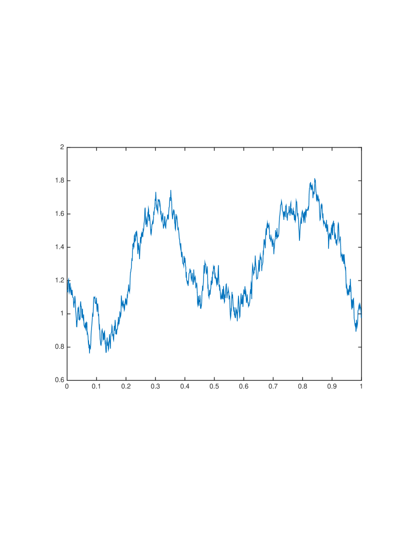
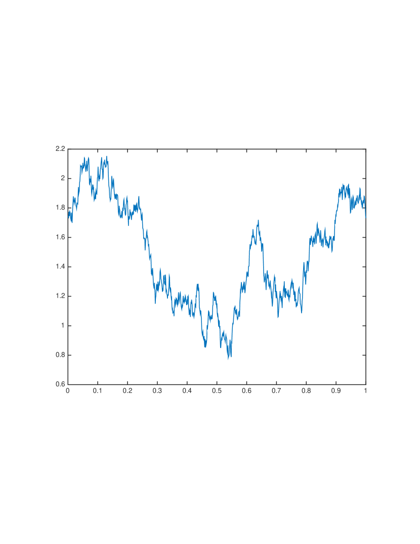
Figure 1. The Brown-Resnick process on $[0,1]$ with Brownian motion input. The grid mesh is 0.001.

Figure 2 presents two samples of the Brown-Resnick random field on $[0,1]^{2}$ when $X$ is a Brownian sheet.

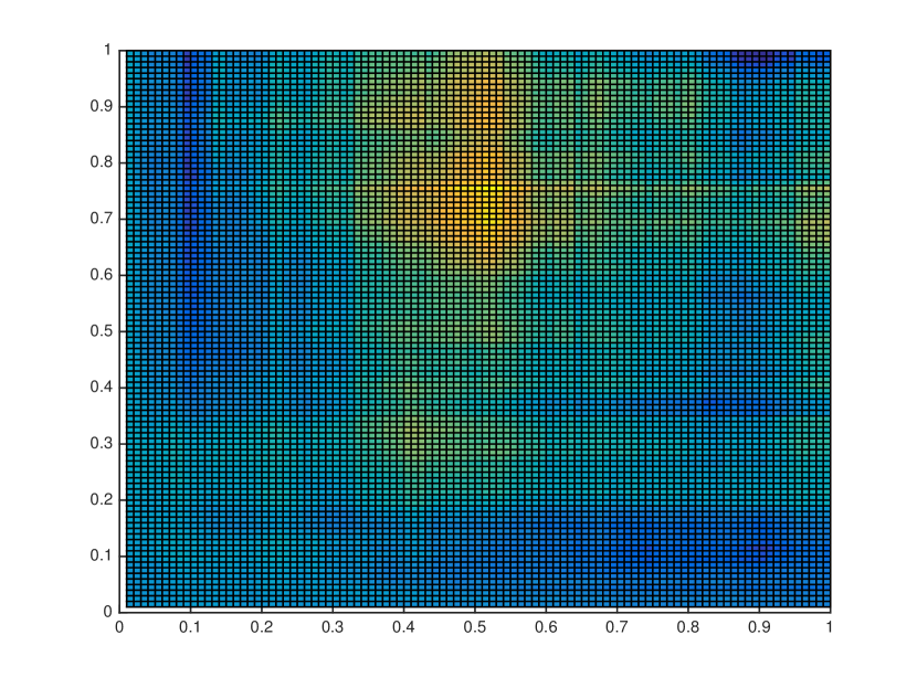
Figure 2. The Brown-Resnick field on $[0,1]^{2}$ with Brownian sheet input. The grid mesh is 0.001.

We validated the implementation of our algorithm by checking the distribution of $\max(M(0.5),M(1))$, which is the maximum of the Brownian-Resnick process at two locations with standard Brownian Motion generator, generated by our algorithm. Note that according to the bivariate Hüsler-Reiss distribution of this process, $\max(M(0.5),M(1))-\log(2\Phi(\sqrt{0.5}/2))$ should have the standard Gumbel distribution. The QQ-plot in Figure 3 confirms empirically that the distribution of $\max(M(0.5),M(1))-\log(2\Phi(\sqrt{0.5}/2))$ is indeed standard Gumbel.

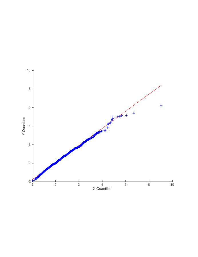
Figure 3. The QQ-plot of $M(0.5)\bigvee M(1)-\log(2\Phi(\sqrt{0.5}/2))$ as generated by our algorithm vs. standard Gumbel

Next we will compare the computational cost in CPU time of our algorithm with the algorithm proposed in [17]. We conducted both algorithms to generate 200 samples of the Brown-Resnick process $M$ with fractional Brownian motion inputs. We recorded both the average CPU time for generating a single sample and the $95\%$ confidence interval for the mean based on our 200 samples, for different grid numbers $d=1000,2000,5000$ and $10000$, and with different Hurst parameters $H\in\left\{1/4,1/2,3/4\right\}$ of the fractional Brownian motion. The sample estimates and the $95\%$ confidence intervals for the mean CPU times to generate a single sample are shown in Table 1. They illustrate that when the number of grids increases, the computational cost of our algorithm appears to increase almost linearly, while the cost for the algorithm proposed in [17] increases quadratically. Because we are using the circulant embedding method to generate the fractional Brownian vectors, which has a complexity of order $O(d\log d)$, it is consistent with expectations. It is worth noting that for this method the computational cost to generate a $d$-dimensional Gaussian vector is the same as for generating a $2^{\lceil\log_{2}d\rceil}$-dimensional Gaussian vector. However, this consideration will not affect our comparison because we used this method in both algorithms.

Average cost per sample (second) (RB)
($\pm$ half-width of confidence interval)
$d$	$H=1/4$	$H=1/2$	$H=3/4$
1000	0.03 $\pm$ 0.003	0.03 $\pm$ 0.002	0.03 $\pm$ 0.001
2000	0.08 $\pm$ 0.020	0.06 $\pm$ 0.007	0.06 $\pm$ 0.002
5000	0.19 $\pm$ 0.071	0.13 $\pm$ 0.004	0.13 $\pm$ 0.008
10000	0.32 $\pm$ 0.027	0.26 $\pm$ 0.009	0.27 $\pm$ 0.008

Average cost per sample (second) (DM)
$d$	$H=1/4$	$H=1/2$	$H=3/4$
1000	0.40 $\pm$ 0.04	0.28 $\pm$ 0.03	0.43 $\pm$ 0.05
2000	1.23 $\pm$ 0.13	1.00 $\pm$ 0.13	1.37 $\pm$ 0.15
5000	7.32 $\pm$ 0.88	4.82 $\pm$ 0.67	5.97 $\pm$ 0.79
10000	28.98 $\pm$ 3.18	21.42 $\pm$ 2.64	19.14 $\pm$ 2.67

Average cost per sample (second) (EF)
$d$	$H=1/4$	$H=1/2$	$H=3/4$
1000	0.15 $\pm$ 0.02	0.13 $\pm$ 0.02	0.15 $\pm$ 0.02
2000	0.49 $\pm$ 0.06	0.46 $\pm$ 0.05	0.66 $\pm$ 0.09
5000	2.83 $\pm$ 0.32	2.34 $\pm$ 0.28	3.39 $\pm$ 0.43
10000	10.81 $\pm$ 1.46	9.67 $\pm$ 1.24	12.17 $\pm$ 1.70

Table 1. Comparison of running time of our algorithm (RB) vs. [17] (DM) vs. [18] (EF).

Next we compare the number of Gaussian vectors generated in our algorithm with the algorithms of [17] and [18]. We generate samples of the Brown-Resnick process with fractional Brownian motion generator, with $H=3/4$. We used the grid numbers $d=1000,3000,5000,7000,9000$. To get comparable relative error, we simulate 1000 times for algorithms DM and EF, and 10000 times for RB. We calculated the sample average of the number of Gaussian vectors generated in each of the algorithms, and the $95\%$ confidence bounds. Table 2 illustrates our main result. On the left, Figure 4 exhibits the plot corresponding to Table 2 for all three algorithms. On the right, Figure 4 focuses on the algorithm RB. The number of Gaussian vectors generated increases linearly in both the algorithms of [17] and [18], with a reduction of constant factor using the extremal function algorithm from [18]. In our algorithm this number stays roughly at the same level.

Number of Gaussian vectors
d	RB	DM	EF
1000	29.5 $\pm$ 2.0	1522.1 $\pm$ 83.3	1040.4 $\pm$ 60.5
3000	28.7 $\pm$ 2.1	4440.1 $\pm$ 248.9	3101.1 $\pm$ 194.2
5000	32.5 $\pm$ 4.2	7648.0 $\pm$ 436.3	5056.3 $\pm$ 298.2
7000	31.4 $\pm$ 2.9	10642.0 $\pm$ 638.4	6961.4 $\pm$ 423.8
9000	26.5 $\pm$ 1.5	13570.0 $\pm$ 796.1	8886.6 $\pm$ 510.3

Table 2. Comparison of number of Gaussian vectors generated in our algorithm (RB) v.s. [17] (DM) v.s. [18] (EF), $H=3/4$.

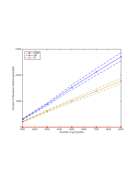
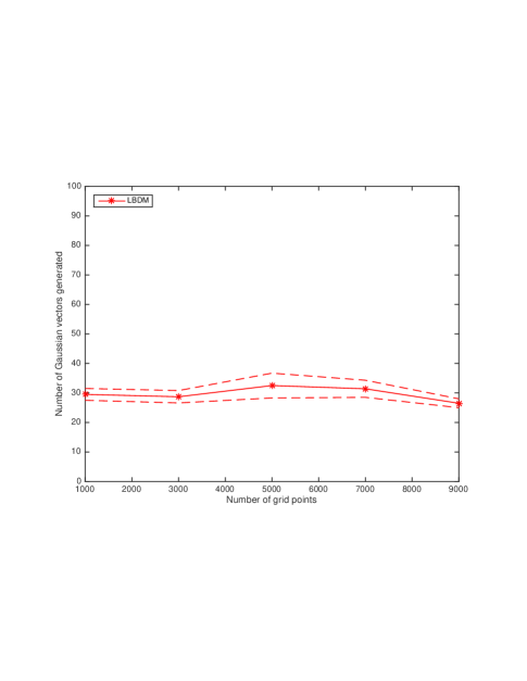
Figure 4. Comparison of number of Gaussian vectors generated in our algorithm (RB) v.s. [17] (DM) v.s. [18] (EF), $H=3/4$.

References

• [1] Adler, R. J. and Taylor, J. E. (2007). Random Fields and Geometry. Springer, New York.
• [2] Asmussen, S. (2003). Applied Probability and Queues, 2nd ed. Springer, New York.
• [3] Asmussen, S. and Glynn, P. (2007). Stochastic Simulation: Algorithms and Analysis. Springer, New York.
• [4] Gut, A. (2009). Stopped Random Walks. Springer, New York.
• [5] Asmussen, S., Glynn, P. and Pitman, J. (1995). Discretization error in simulation of one-dimensional reflecting Brownian motion. The Annals of Applied Probability, 5(4), 875–896.
• [6] Ayache, A. and Taqqu, M.S. (2003) Rate optimality of wavelet series approximations of fractional Brownian motion. The Journal of Fourier Analysis and Applications, 9, 451–471.
• [7] Blanchet, J. and Chen, X. (2015). Steady-state simulation of reflected Brownian motion and related stochastic networks. The Annals of Applied Probability, 25(6), 3209–3250.
• [8] Blanchet, J. and Chen, X. (2016). Perfect sampling of generalized Jackson networks. arXiv:1601.05499 [math]. http://arxiv.org/abs/1601.05499
• [9] Blanchet, J., Chen, X. and Dong, J. (2014). $\epsilon$-Strong simulation for multidimensional stochastic differential equations via rough path analysis. To appear in Annals of Applied Probability. http://arxiv.org/abs/1403.5722
• [10] Blanchet, J. and Dong, J. (2012). Sampling point processes on stable unbounded regions and exact simulation of queues. In Simulation Conference (WSC), Proceedings of the 2012 Winter (pp. 1–12). IEEE. This reference is incomplete
• [11] Blanchet, J. and Dong, J. (2015). Perfect sampling for infinite server and loss systems. Advances in Applied Probability, 47(3), 761–786.
• [12] Blanchet, J., Dong, J. and Pei, Y. (2015). Perfect sampling of GI/GI/c queues. It is uncommon to say where the paper has been submitted Submitted to Queueing Systems: Theory and Applications.
• [13] Blanchet, J. and Wallwater, A. (2015). Exact sampling of stationary and time reversed queues. ACM Transactions on Modeling and Computer Simulation (TOMACS), 25(4), Article 26.
• [14] Blanchet, J. and Sigman, K. (2011). On exact sampling of stochastic perpetuities. Journal of Applied Probability, 48A, 165–182.
• [15] Brown, B. M. and Resnick, S. I.. (1977). Extreme values of independent stochastic processes. Journal of Applied Probability, 14(4), 732–739.
• [16] Buishand, T. A., de Haan, L., and Zhou, C. (2008). On spatial extremes: With application to a rainfall problem. The Annals of Applied Statistics, 2(2), 624–642.
• [17] Dieker, A. B. and Mikosch, T. (2015). Exact simulation of Brown-Resnick random fields at a finite number of locations. Extremes, 18(2), 301–314.
• [18] Dombry, C., Engelke, S. and Oesting, M. (2015). Exact simulation of max-stable processes. arXiv:1506.04430.
• [19] Embrechts, P., Klüppelberg, C. and Mikosch (1997). Modelling Extremal Events for Insurance and Finance. Springer, New York.
• [20] Haan, L. de and Zhou, C. (2008). On extreme value analysis of a spatial process. RevStat - Statistical Journal, 6(1), 71–81.
• [21] Haan, L. de (1984). A spectral representation for max-stable processes. The Annals of Probability, 12(4), 1194–1204.
• [22] Hoffman, Y., Ribak, E. (1991). Constrained realizations of Gaussian fields - a simple algorithm. The Astrophysical Journal, vol. 380, pp. L5–L8.
• [23] Kabluchko, Z., Schlather, M. and Haan, L. de (2009). Stationary max-stable fields associated to negative definite functions. The Annals of Probability, 37(5), 2042–2065.
• [24] Kenealy, B. (2013, August 11). New York’s MTA buys $200 million cat bond to avoid storm surge losses. Business Insurance. Retrieved from https://www.businessinsurance.com
• [25] Kühn, T. and Linde, W. (2002). Optimal series representation of fractional Brownian sheets. Bernoulli, 8(5), 669–696.
• [26] Oesting, M., Schlather, M. and Zhou, C. (2017). Exact and fast simulation of max-stable processes on a compact set using the normalized spectral representation. To appear in Bernoulli.
• [27] Pollock, M., Johansen, A. M. and Roberts, G. O. (2016). On the exact and $\epsilon$-strong simulation of (jump) diffusions. Bernoulli, 22(2), 794–856.
• [28] Schilling, R. L. and Partzsch, L. (2012) Brownian Motion. An Introduction to Stochastic Processes. De Gruyter, Berlin/Boston.
• [29] Schlather, M. (2002). Models for stationary max-stable random fields. Extremes, 5(1), 33–44.
• [30] Smith, R. L. (1990). Max-stable processes and spatial extremes. Unpublished manuscript, Univer.
• [31] Steele, J. M. (2001). Stochastic Calculus and Financial Applications. Springer, New York.
• [32] Thibaud, E., Aalto, J., Cooley, D. S., Davison, A. C. and Heikkinen, J. (2015). Bayesian inference for the Brown-Resnick process, with an application to extreme low temperatures. arXiv:1506.07836.
• [33] Vaart, A. van der and Wellner, J. A. (1996). Weak Convergence and Empirical Processes. With Applications to Statistics. Springer, New York.