Max-affine estimators for convex stochastic programming

Abstract

In this paper, we consider two sequential decision making problems with a convexity structure, namely an energy storage optimization task and a multi-product assembly example. We formulate these problems in the stochastic programming framework and discuss an approximate dynamic programming technique for their solutions. As the cost-to-go functions are convex in these cases, we use max-affine estimates for their approximations. To train such a max-affine estimate, we provide a new convex regression algorithm, and evaluate it empirically for these planning scenarios.

1 Introdution

This paper considers multi-stage stochastic programming problems (e.g., Shapiro et al., 2009; Birge and Louveaux, 2011) with restricting the model so that the cost-to-go functions remain convex (Section 2). To motivate this framework, we provide two realistic benchmark planning problems (Section 5), namely solar energy production with storage, and the operation of a beer brewery.

To address these problems, we consider an approximate dynamic programming approach (e.g., Bertsekas, 2005; Powell, 2011). For this, we estimate the cost-to-go functions by convex regression techniques using max-affine representations (formed by the maximum of finitely many affine functions). To train a max-affine estimator, we propose a novel algorithm (AMAP, Section 3), which combines ideas of the convex adaptive partitioning method (CAP, Hannah and Dunson, 2013) and the least squares partition algorithm (LSPA, Magnani and Boyd, 2009), while learns the model size by cross-validation.

We discuss a full approximate dynamic programming approach (Section 4) that estimates the cost-to-go functions globally. It uses a forward pass to generate a data set for the cost-to-go estimation by uniformly sampling the reachable decision space. Then it performs a backward pass to recursively approximate the cost-to-go functions for all stages. The technical details of this algorithm is provided for polyhedral decision sets and convex piecewise-linear cost-to-go representations.

Finally, we evaluate max-affine estimators in the contexts of our benchmark planning problems through the full approximate dynamic programming algorithm (Section 5).

2 Convex stochastic programming

Consider a $T$-stage stochastic programming (SP) problem (e.g., Ruszczyński and Shapiro, 2003; Shapiro et al., 2009; Birge and Louveaux, 2011), where the goal is to find a decision ${\bm{x}}_{1}^{*}$ solving the following:

$$\begin{split}{\bm{x}}_{1}^{*}\in\mathop{\mathrm{argmin}}_{{\bm{x}}_{1}\in\mathbb{X}_{1}({\bm{x}}_{0},{\bm{z}}_{0})}&J_{1}({\bm{x}}_{1})\,,\quad J_{t}({\bm{x}}_{t})\doteq\mathbb{E}\Big{[}c_{t}({\bm{x}}_{t},{\bm{\mathcal{Z}}}_{t})+\min_{{\bm{x}}_{t+1}\in\mathbb{X}_{t+1}({\bm{x}}_{t},{\bm{\mathcal{Z}}}_{t})}J_{t+1}({\bm{x}}_{t+1})\Big{]}\,,\end{split}$$ (1)

with $t=1,\ldots,T$, some fixed initial values ${\bm{x}}_{0},{\bm{z}}_{0}$, $\mathbb{X}_{T+1}({\bm{x}}_{T},{\bm{\mathcal{Z}}}_{T})\doteq\{\bot\}$, $J_{T+1}(\bot)\doteq 0$, and a sequence of independent random variables ${\bm{\mathcal{Z}}}_{1},\ldots,{\bm{\mathcal{Z}}}_{T}$.

Notice that (1) includes discrete-time finite-horizon Markov decision process formulations (e.g., Puterman, 1994; Sutton, 1998; Bertsekas, 2005; Szepesvári, 2010; Powell, 2011) after the state and action variables are combined into a single decision variable ${\bm{x}}_{t}$, and the environment dynamics along with the action constraints are described by the decision constraint functions $\mathbb{X}_{t}$.

In this text, we consider only a subset of SP problems (1) when the cost functions $c_{1},\ldots,c_{T}$ are convex in ${\bm{x}}_{t}$, and $\textrm{graph}(\mathbb{X}_{t}({\bm{x}}_{t},{\bm{\mathcal{Z}}}_{t}))$ are convex sets for all $t=1,\ldots,T$ and all ${\bm{\mathcal{Z}}}_{t}$ realizations, where the graph of a set-valued function $C:\mathbb{X}\to 2^{\mathbb{Y}}$ is defined as $\textrm{graph}(C)\doteq\big{\{}({\bm{x}},{\bm{y}})\in\mathbb{X}\times\mathbb{Y}:{\bm{y}}\in C({\bm{x}})\big{\}}$. In this case, the cost-to-go functions $J_{t}(\cdot)$ are convex for all $t=1,\ldots,T$ (e.g., see Lemma 1), hence we call these SP problems convex.

One approach to deal with such SP problems (1) is to use approximate dynamic programming (ADP) methods (e.g., Bertsekas, 2005; Powell, 2011; Birge and Louveaux, 2011; Hannah et al., 2014) which construct nested approximations to the cost-to-go functions,

$$\hat{J}_{t}({\bm{x}}_{t})\approx\mathbb{E}\left[c_{t}({\bm{x}}_{t},{\bm{\mathcal{Z}}}_{t})+\min_{{\bm{x}}_{t+1}\in\mathbb{X}_{t+1}({\bm{x}}_{t},{\bm{\mathcal{Z}}}_{t})}\hat{J}_{t+1}({\bm{x}}_{t+1})\right]\approx J_{t}({\bm{x}}_{t})\,,$$ (2)

backwards for $t=T,T-1,\ldots,1$. Notice that for convex SP problems with convex cost-to-go functions $J_{t}$, the estimates $\hat{J}_{t}$ can be restricted to be convex without loss of generality, and so the minimization tasks in (2) can be solved efficiently.

3 Adaptive max-affine partitioning algorithm

To represent convex cost-to-go functions, we use max-affine maps formed by the maximum of finitely many affine functions (hyperplanes). To train the parameters of such a max-affine estimate, we present a new convex regression algorithm called Adaptive Max-Affine Partitioning (AMAP), which combines the partitioning technique of the convex adaptive partitioning algorithm (CAP, Hannah and Dunson, 2013), the least squared partition algorithm (LSPA, Magnani and Boyd, 2009), and learns the model size (number of hyperplanes) by a cross-validation scheme.

Just as LSPA and CAP, AMAP also aims to reduce the empirical risk with respect to the squared loss defined as $R_{n}(f)\doteq\frac{1}{n}\sum_{i=1}^{n}|f({\bm{x}}_{i})-y_{i}|^{2}$ for some function $f$ and data set $\mathcal{D}_{n}\doteq\{({\bm{x}}_{i},y_{i}):i=1,\ldots,n\}\subseteq(\mathbb{R}^{d}\times\mathbb{R})^{n}$ with $n$ samples and dimension $d$. For the discussion of AMAP, denote the max-affine function of model $M=\{({\bm{a}}_{k},b_{k}):k=1,\ldots,K\}$ by $f_{M}({\bm{x}})\doteq\max_{k=1,\ldots,K}{\bm{a}}_{k}^{\top}{\bm{x}}+b_{k}$ for ${\bm{x}}\in\mathbb{R}^{d}$. Notice that each max-affine model $M$ induces a partition over the data set $\mathcal{D}_{n}$ as

$$\begin{split}P&\doteq\{\mathcal{C}_{1},\ldots,\mathcal{C}_{K}\}\,,\quad\mathcal{C}_{k}\doteq\big{\{}i\in\{1,\ldots,n\}\,\big{|}\,{\bm{x}}_{i}^{\top}{\bm{a}}_{k}+b_{k}=f_{M}({\bm{x}}_{i})\big{\}}\,,\end{split}$$ (3)

for some $K\in\mathbb{N}$ and all $k=1,\ldots,K$, where ties are broken arbitrarily so that $\mathcal{C}_{k}\neq\emptyset$ and $\mathcal{C}_{k}\cap\mathcal{C}_{l}\neq\emptyset\iff k=l$ for all $k,l=1,\ldots,K$. Furthermore, each partition $P$ induces a max-affine model by fitting each cell of $P$ using the linear least squares algorithm:

$$\begin{split}M&\doteq\{({\bm{a}}_{k},b_{k}):k=1,\ldots,K\}\,,\quad\Delta_{ik}\doteq{\bm{x}}_{i}-\frac{1}{|\mathcal{C}_{k}|}\sum_{i\in\mathcal{C}_{k}}{\bm{x}}_{i}\,,\\ {\bm{a}}_{k}&\doteq\Big{(}\sum_{i\in\mathcal{C}_{k}}\Delta_{ik}\Delta_{ik}^{\top}+\beta I_{d}\Big{)}^{-1}\sum_{i\in\mathcal{C}_{k}}\Delta_{ik}\,y_{i}\,,\quad b_{k}\doteq\frac{1}{|\mathcal{C}_{k}|}\sum_{i\in\mathcal{C}_{k}}y_{i}-{\bm{a}}_{k}^{\top}{\bm{x}}_{i}\,,\end{split}$$ (4)

where $I_{d}$ is the $d\times d$ identity matrix, and $\beta>0$ is set to some small value for stability (we use $\beta\doteq 10^{-6}$).

Similar to CAP, AMAP builds the model incrementally by cell splitting, and improves the partition using LSPA by alternating steps (3) and (4). The AMAP model improvement step is given by Algorithm 1.

1.  input:  training set $\mathcal{D}_{n}$, model $M=\{({\bm{a}}_{k},b_{k}):k=1,\ldots,K\}$,

1.               partition $P=\{\mathcal{C}_{1},\ldots,\mathcal{C}_{K}\}$, empirical risk $E$, minimum cell size $s_{*}$

1.   {cell splitting}

2.   $M_{*}^{\prime}\leftarrow M,E_{*}^{\prime}\leftarrow E$, $P_{*}^{\prime}\leftarrow P$

3.  for all $k=1,\ldots,K$ do

4.     if $|\mathcal{C}_{k}|\geq 2s_{*}$ then

5.        for all $j=1,\ldots,d$ do

6.            $m_{j}\leftarrow\textrm{median}(\{\mathcal{X}_{ij}:i\in\mathcal{C}_{k}\})$

7.            $\mathcal{C}_{\textrm{le}}\leftarrow\{i\in\mathcal{C}_{k}:\mathcal{X}_{ij}\leq m_{j}\}$, $\mathcal{C}_{\textrm{gt}}\leftarrow\{i\in\mathcal{C}_{k}:\mathcal{X}_{ij}\geq m_{j}\}$

8.            $({\bm{a}}_{\textrm{le}},b_{\textrm{le}})\leftarrow$ least squares on $\{({\bm{\mathcal{X}}}_{i},\mathcal{Y}_{i}):i\in\mathcal{C}_{\textrm{le}}\}$

9.            $({\bm{a}}_{\textrm{gt}},b_{\textrm{gt}})\leftarrow$ least squares on $\{({\bm{\mathcal{X}}}_{i},\mathcal{Y}_{i}):i\in\mathcal{C}_{\textrm{gt}}\}$

10.            $M^{\prime}\leftarrow\big{(}M\setminus\{({\bm{a}}_{k},b_{k})\}\big{)}\cup\{({\bm{a}}_{\textrm{le}},b_{\textrm{le}}),({\bm{a}}_{\textrm{gt}},b_{\textrm{gt}})\}$

11.            $E^{\prime}\leftarrow R_{n}\big{(}f_{M^{\prime}}(\cdot)\big{)}$

12.           if $E^{\prime}<E_{*}^{\prime}$ then

13.              $M_{*}^{\prime}\leftarrow M^{\prime}$, $E_{*}^{\prime}\leftarrow E^{\prime}$, $P_{*}^{\prime}\leftarrow(P\setminus\{\mathcal{C}_{k}\})\cup\{\mathcal{C}_{\textrm{le}},\mathcal{C}_{\textrm{gt}}\}$

14.           end if

15.        end for

16.     end if

17.  end for

17.   {running LSPA}

18.  repeat

19.      $M_{*}\leftarrow M_{*}^{\prime}$, $E_{*}\leftarrow E_{*}^{\prime}$, $P_{*}\leftarrow P_{*}^{\prime}$

20.     $P_{*}^{\prime}\leftarrow$ induced partition of $M_{*}$ by (3)

21.      $M_{*}^{\prime}\leftarrow$ fitting of partition $P_{*}^{\prime}$ by (4)

22.      $E_{*}^{\prime}\leftarrow R_{n}\big{(}f_{M^{\prime}_{*}}(\cdot)\big{)}$

23.  until $\min_{\mathcal{C}\in P_{*}^{\prime}}|\mathcal{C}|\geq s_{*}$ and $E_{*}^{\prime}<E_{*}$

24.  output:  model $M_{*}$, partition $P_{*}$, empirical risk $E_{*}$

Algorithm 1: AMAP model improvement step.

Notice that AMAP performs coordinate-wise cell splitting (steps 5 to 15), just as CAP, however, AMAP makes the split always at the median (steps 6 and 7) instead of checking multiple cut points. This saves computation time, but can also create worse splits. To compensate for this loss in quality, AMAP runs a restricted version of LSPA (steps 18 to 23) not just for a single step as CAP, but until the candidate model improves the empirical risk and its induced partition satisfies the minimum cell requirement (step 23). We also mention that indices $\{i\in\mathcal{C}_{k}:\mathcal{X}_{ij}=m_{j}\}$ are assigned to $\mathcal{C}_{\textrm{le}}$ and $\mathcal{C}_{\textrm{gt}}$ (step 7) in order to preserve the minimum cell requirement.

Notice that the difference between $M^{\prime}$ and $M$ is only two hyperplanes (step 10), so the number of arithmetic operations for computing $E^{\prime}$ (step 11) can be improved from $O(nKd)$ to $O(nd)$. Further, the cost of least squares regressions (steps 8 and 9) is $O(|\mathcal{C}_{k}|d^{2})$. Hence, the computational cost of the entire cell splitting process (steps 2 to 17) is bounded by $O(\max\{K,d\}d^{2}n)$. For the LSPA part, the partition fitting (step 21) is $O(nd^{2})$ and the error calculation (step 22) is $O(nKd)$. So, the cost of a single LSPA iteration (steps 19 to 22) is bounded by $O(\max\{K,d\}dn)$, implying that the cost of Algorithm 1 is bounded by $O\big{(}\max\{t_{\textrm{LSPA}},d\}\max\{K,d\}dn\big{)}$, where $t_{\textrm{LSPA}}$ denotes the number of LSPA iterations.

Undesirably, coordinate-wise cell splitting does not provide rotational invariance. To fix this, we run AMAP after a pre-processing step, which uses thin singular value decomposition (thin-SVD) to drop redundant coordinates and align the data along a rotation invariant basis. Formally, let the raw (but already centered) data be organized into $X\in\mathbb{R}^{n\times d}$ and ${\bm{y}}\in\mathbb{R}^{n}$. Then, we scale the values $[y_{1}\ldots y_{n}]^{\top}\doteq{\bm{y}}/\max\{1,\left\lVert{\bm{y}}\right\rVert_{\infty}\}$, and decompose $X$ by thin-SVD as $X=USV^{\top}$, where $U\in\mathbb{R}^{n\times d}$ is semi-orthogonal, $S\in\mathbb{R}^{d\times d}$ is diagonal with singular values in decreasing order, and $V\in\mathbb{R}^{d\times d}$ is orthogonal. Coordinates related to zero singular values are dropped and the points are scaled by $S$ as $[{\bm{x}}_{1}\ldots{\bm{x}}_{n}]^{\top}\doteq US/\max\{1,S_{11}\}$, where $S_{11}$ is the largest singular value. Now observe that rotating the raw points $X$ as $XQ$ with some orthogonal matrix $Q\in\mathbb{R}^{d\times d}$ only transforms $V$ to $Q^{\top}V$ and does not affect the pre-processed points ${\bm{x}}_{1},\ldots,{\bm{x}}_{n}$. Finally, we note that thin-SVD can be computed using $O(nd^{2})$ arithmetic operations (with $n\geq d)$, which is even less than the asymptotic cost of Algorithm 1.

AMAP is presented as Algorithm 2 and run using uniformly shuffled (and pre-processed) data $\mathcal{D}_{n}$, and a partition $\{F_{1},\ldots,F_{u_{*}}\}$ of $\{1,\ldots,n\}$ with equally sized cells (the last one might be smaller) defining the cross-validation folds.

1.  input:  training set $\mathcal{D}_{n}$, minimum cell size $s_{*}$, folds $F_{1},\ldots,F_{u_{*}}$, iterations $t_{\textrm{wait}}$

1.   {initialization}

2.  for $u=1,\ldots,u_{*}$ do

3.     $P_{u}\leftarrow\{\mkern 4.0mu\overline{\mkern-4.0muF\mkern 0.0mu}\mkern-3.0mu_{u}\}$ with $\mkern 4.0mu\overline{\mkern-4.0muF\mkern 0.0mu}\mkern-3.0mu_{u}\doteq\{1,\ldots,n\}\setminus F_{u}$

4.     $M_{u}=\{({\bm{a}}_{1}^{u},b_{1}^{u})\}\leftarrow$ least squares on $\{({\bm{x}}_{i},y_{i}):i\in\mkern 4.0mu\overline{\mkern-4.0muF\mkern 0.0mu}\mkern-3.0mu_{u}\}$

5.     $\mkern 4.0mu\overline{\mkern-4.0muE\mkern 0.0mu}\mkern-1.0mu_{u}\leftarrow|\mkern 4.0mu\overline{\mkern-4.0muF\mkern 0.0mu}\mkern-3.0mu_{u}|^{-1}\sum_{i\in\mkern 4.0mu\overline{\mkern-4.0muF\mkern 0.0mu}\mkern-3.0mu_{u}}|f_{M_{u}}({\bm{x}}_{i})-y_{i}|^{2}$, $E_{u}\leftarrow|F_{u}|^{-1}\sum_{i\in F_{u}}|f_{M_{u}}({\bm{x}}_{i})-y_{i}|^{2}$

6.  end for

7.   $\mathcal{M}_{*}\leftarrow\{M_{1},\ldots,M_{u_{*}}\}$, $E_{*}\leftarrow\frac{1}{u_{*}}\sum_{u=1}^{u_{*}}E_{u}$

7.   {cross-validation training}

8.   $t\leftarrow 1$, $t_{\max}\leftarrow t_{\textrm{wait}}$

9.  while $t\leq\min\{t_{\max},\lceil n^{d/(d+4)}\rceil\}$ do

10.     for $u=1,\ldots,u_{*}$ do

11.         $(M_{u},P_{u},\mkern 4.0mu\overline{\mkern-4.0muE\mkern 0.0mu}\mkern-1.0mu_{u})\leftarrow$ update by Algorithm 1 using $\{({\bm{x}}_{i},y_{i}):i\in\mkern 4.0mu\overline{\mkern-4.0muF\mkern 0.0mu}\mkern-3.0mu_{u}\}$, $M_{u}$, $P_{u}$, $\mkern 4.0mu\overline{\mkern-4.0muE\mkern 0.0mu}\mkern-1.0mu_{u}$, $s_{*}$

12.         $E_{u}\leftarrow|F_{u}|^{-1}\sum_{i\in F_{u}}|f_{M_{u}}({\bm{x}}_{i})-y_{i}|^{2}$

13.     end for

14.      $E\leftarrow\frac{1}{u_{*}}\sum_{u=1}^{u_{*}}E_{u}$

15.     if $E<E_{*}$ then

16.         $\mathcal{M}_{*}\leftarrow\{M_{1},\ldots,M_{u_{*}}\}$, $E_{*}\leftarrow E$, $t_{\max}\leftarrow t+t_{\textrm{wait}}$

17.     end if

18.     $t\leftarrow t+1$

19.  end while

19.   {choosing the final model}

20.   $M_{*}\leftarrow\mathop{\mathrm{argmin}}_{M\in\mathcal{M}_{*}}R_{n}\big{(}f_{M}(\cdot)\big{)}$

21.  output:  model $M_{*}$

Algorithm 2: Adaptive max-affine partitioning (AMAP).

For model selection, AMAP uses a $u_{*}$-fold cross-validation scheme (steps 8 to 19) to find an appropriate model size that terminates when the cross-validation error (step 14) of the best model set $\mathcal{M}_{*}$ (steps 7 and 16) cannot be further improved for $t_{\textrm{wait}}$ iterations. At the end, the final model is chosen from the model set $\mathcal{M}_{*}$ having the best cross-validation error, and selected so to minimize the empirical risk on the entire data (step 20). For this scheme, we use the parameters $u_{*}\doteq 10$ and $t_{\textrm{wait}}\doteq 5$.

AMAP starts with models having a single hyperplane (steps 2 to 6) and increments each model by at most one hyperplane in every iteration (step 11). Notice that if AMAP cannot find a split for a model $M_{u}$ to improve the empirical risk $\mkern 4.0mu\overline{\mkern-4.0muE\mkern 0.0mu}\mkern-1.0mu_{u}$, the update for model $M_{u}$ (steps 11 and 12) can be skipped in the subsequent iterations as Algorithm 1 is deterministic. We also mention that for the minimum cell size, we use $s_{*}\doteq\max\{2(d+1),\lceil\log_{2}(n)\rceil\}$ allowing model sizes up to $O\big{(}n^{d/(d+4)}/\ln(n)\big{)}$, which is enough for near-optimal worst-case performance (Balázs et al., 2015, Theorems 4.1 and 4.2).

4 Approximate dynamic programming

Here we use max-affine estimators to approximate the cost-to-go functions of convex SP problems. First, notice that solving (1) is equivalent to the computation of $\pi_{1}({\bm{x}}_{0},{\bm{z}}_{0})$, where

$$\begin{split}\pi_{t}({\bm{x}}_{t-1},{\bm{z}}_{t-1})&\doteq\mathop{\mathrm{argmin}}_{{\bm{x}}_{t}\in\mathbb{X}_{t}({\bm{x}}_{t-1},{\bm{z}}_{t-1})}J_{t}({\bm{x}}_{t})\,,\\ J_{t}({\bm{x}}_{t})&=\mathbb{E}\big{[}c_{t}({\bm{x}}_{t},{\bm{\mathcal{Z}}}_{t})+J_{t+1}(\pi_{t+1}({\bm{x}}_{t},{\bm{\mathcal{Z}}}_{t}))\big{]}\,,\end{split}$$ (5)

for all $t=1,\ldots,T$, and $\pi_{T+1}(\cdot,\cdot)\doteq\bot$ with $J_{T+1}(\bot)=0$. The sequence $\pi\doteq(\pi_{1},\ldots,\pi_{T})$ represents an optimal policy.

We only consider SP problems with convex polyhedral decision constraints written as $\mathbb{X}_{t+1}({\bm{x}}_{t},{\bm{\mathcal{Z}}}_{t})=\{{\bm{x}}_{t+1}:Q_{t+1}{\bm{x}}_{t+1}+W_{t+1}({\bm{\mathcal{Z}}}_{t}){\bm{x}}_{t}\leq{\bm{c}}_{t+1}({\bm{\mathcal{Z}}}_{t})\}$ which are non-empty for all possible realizations of ${\bm{x}}_{t}$ and ${\bm{\mathcal{Z}}}_{t}$. As the coefficient $Q_{t+1}$ of the decision variable ${\bm{x}}_{t+1}$ is independent of random disturbances ${\bm{\mathcal{Z}}}_{t}$ and the constraint ${\bm{x}}_{t}\in\mathbb{X}_{t}({\bm{x}}_{t-1},{\bm{z}}_{t-1})$ for policy $\pi_{t}$ is feasible for any ${\bm{x}}_{t-1}$ and ${\bm{z}}_{t-1}$, these SP problems are said to have a fixed, relatively complete recourse (Shapiro et al., 2009, Section 2.1.3). We will exploit the fixed recourse property for sampling (6), while relatively complete recourse allows us not to deal with infeasibility issues which could make these problems very difficult to solve.

In order to construct an approximation $\hat{J}_{t}$ to the cost-to-go function $J_{t}$, we need “realizable” decision samples ${\bm{x}}_{t,i}$ at stage $t$. We generate these incrementally during a forward pass for $t=1,2,\ldots,T$, where given $n$ decisions ${\bm{x}}_{t,1},\ldots,{\bm{x}}_{t,n}$ and $m$ disturbances ${\bm{z}}_{t,1},\ldots,{\bm{z}}_{t,m}$ at stage $t$, we uniformly sample new decisions for stage $t+1$ from the set

$$\begin{split}\hat{\mathbb{X}}_{t+1}&\doteq\textrm{conv}\bigg{(}\bigcup_{i=1,\ldots,n,\atop j=1,\ldots,m}\mathbb{X}_{t+1}({\bm{x}}_{t,i},{\bm{z}}_{t,j})\bigg{)}\\ &=\Big{\{}{\bm{x}}_{t+1}:Q_{t+1}{\bm{x}}_{t+1}\leq\max_{i=1,\ldots,n,\atop j=1,\ldots,m}\big{\{}{\bm{c}}_{t+1}({\bm{z}}_{t,j})-W_{t+1}({\bm{z}}_{t,j}){\bm{x}}_{t,i}\big{\}}\Big{\}}\,,\end{split}$$ (6)

where $\textrm{conv}(\cdot)$ refers to the convex hull of a set, and the maximum is taken component-wise. To uniformly sample the convex polytope $\hat{\mathbb{X}}_{t+1}$, we use the Hit-and-run Markov-Chain Monte-Carlo algorithm (Smith, 1984, or see Vempala, 2005) by generating 100 chains (to reduce sample correlation) each started from the average of 10 randomly generated border points, and discarding $d_{t+1}^{2}$ samples on each chain during the burn-in phase, where $d_{t+1}$ is the dimension of ${\bm{x}}_{t+1}$.

Then, during a backward pass for $t=T,T-1,\ldots,1$, we recursively use the cost-to-go estimate of the previous stage $\hat{J}_{t+1}(\cdot)$ to approximate the values of the cost-to-go function $J_{t}$ at the decision samples ${\bm{x}}_{t,i}$ generated during the forward pass, that is

$$J_{t}({\bm{x}}_{t,i})\approx y_{t,i}\doteq\frac{1}{m}\sum_{j=1}^{m}c_{t}({\bm{x}}_{t,i},{\bm{z}}_{t,j})+\min_{{\bm{x}}_{t+1}\in\mathbb{X}_{t+1}({\bm{x}}_{t,i},{\bm{z}}_{t,j})}\hat{J}_{t+1}({\bm{x}}_{t+1})$$ (7)

for all $t=1,\ldots,T$, and $\hat{J}_{T+1}(\cdot)\equiv 0$. This allows us to set up a regression problem with data $\{({\bm{x}}_{t,i},y_{t,i}):i=1,\ldots,n\}$, and to construct an estimate $\hat{J}_{t}(\cdot)$ of the cost-to-go $J_{t}(\cdot)$.

We call the resulting method, shown as Algorithm 3, full approximate dynamic programming (fADP) because it constructs global approximations to the cost-to-go functions.

1.  input:  SP problem, trajectory count $n$, evaluation count $m$, estimator REG

2.  ${\bm{x}}_{0,i}\leftarrow{\bm{x}}_{0}$ for all $i=1,\ldots,n$

3.  ${\bm{z}}_{0,j}\leftarrow{\bm{z}}_{0}$ for all $j=1,\ldots,m$

3.   {forward pass}

4.  for all $t=0,1,\ldots,T-1$ do

5.     sample ${\bm{x}}_{t+1,1},\ldots,{\bm{x}}_{t+1,n}$ from $\hat{\mathbb{X}}_{t+1}$ by (6) using ${\bm{x}}_{t,1},\ldots,{\bm{x}}_{t,n}$, and ${\bm{z}}_{t,1},\ldots,{\bm{z}}_{t,m}$

6.     sample ${\bm{z}}_{t+1,1},\ldots,{\bm{z}}_{t+1,m}$ from the distribution of ${\bm{\mathcal{Z}}}_{t+1}$

7.  end for

7.   {backward pass}

8.  $\hat{J}_{T+1}(\cdot)\leftarrow 0$

9.  for all $t=T,T-1,\ldots,1$ do

10.     compute $y_{t,1},\ldots,y_{t,n}$ by (7) using $\hat{J}_{t+1}(\cdot)$, ${\bm{x}}_{t,1},\ldots,{\bm{x}}_{t,n}$, and ${\bm{z}}_{t,1},\ldots,{\bm{z}}_{t,m}$

11.     $\hat{J}_{t}(\cdot)\leftarrow\textrm{REG}(\{({\bm{x}}_{t,i},y_{t,i}):i=1,\ldots,n\})$

12.  end for

13.  output:  cost-to-go functions $\hat{J}_{t}(\cdot)$, $t=1,\ldots,T$

Algorithm 3: Full approximate dynamic programming (fADP).

When the cost-to-go functions $J_{t}$ are approximated by “reasonably sized” convex piecewise linear representations $\hat{J}_{t}$, the minimization problem in (7) can be solved efficiently by linear programming (LP). In the following sections, we exploit the speed of LP solvers for fADP using either AMAP or CAP as the regression procedure. Then, the computational cost to run Algorithm 3 is mostly realized by solving $Tnm$ LP tasks for (7) and training $T$ estimators using the regression algorithm REG.

Here we mention that max-affine estimators using as many hyperplanes as the sample size $n$ can be computed by convex optimization techniques efficiently up to a few thousand samples (Mazumder et al., 2015). These estimators provide worst-case generalization error guarantees, however, the provided max-affine models are large enough to turn the LP tasks together too costly to solve (at least using our hardware and implementation). color=blue!20!white,]BG: Future work for tuning LP methods for solving large number of similar tasks. There is some literature on this (as mentioned at the end of the section), see Gassmann and Wallace (1996). But commercial solvers do not provide much support.

The situation is even worse for nonconvex estimators REG for which LP has to be replaced for (7) by a much slower nonlinear constrained optimization method using perhaps randomized restarts to minimize the chance of being trapped in a local minima. Furthermore, when the gradient information with respect to the input is not available (as for many implementations), the minimization over these representations require an even slower gradient-free nonlinear optimization technique. Hence, multivariate adaptive regression splines, support vector regression, and neural networks were impractical to use for fADP on our test problems.

5 Experiments

To test fADP using max-affine estimators, we consider two SP planning problems, namely solar energy production with storage management (Section 5.1), and the operation of a beer brewery (Section 5.2).

For our numerical experiments, the hardware has a Dual-Core AMD Opteron(tm) Processor 250 (2.4GHz, 1KB L1 Cache, 1MB L2 Cache) with 8GB RAM. The software uses MATLAB (R2010b), and the MOSEK Optimization Toolbox (v7.139).

To measure the performance of the fADP algorithm, we evaluate the greedy policy with respect to the learned cost-to-go functions $\{\hat{J}_{t}:t=1,\ldots,T\}$. More precisely, we run $\hat{\pi}\doteq(\hat{\pi}_{1},\ldots,\hat{\pi}_{T})$ with $\hat{\pi}_{t}({\bm{x}}_{t-1},{\bm{z}}_{t-1})\in\mathop{\mathrm{argmin}}_{{\bm{x}}_{t}\in\mathbb{X}_{t}({\bm{x}}_{t-1},{\bm{z}}_{t-1})}\hat{J}_{t}({\bm{x}}_{t})$ on $1000$ episodes, and record the average revenue (negative cost) as $\textrm{REV}\doteq-\frac{1}{1000}\sum_{e=1}^{1000}\sum_{t=1}^{T}c_{t}\big{(}{\bm{x}}^{(e)}_{t},{\bm{z}}^{(e)}_{t}\big{)}$ over the episodes’ trajectories $\big{\{}\big{(}{\bm{x}}^{(e)}_{t},{\bm{z}}^{(e)}_{t}\big{)}:t=1,\ldots,T\big{\}}$, $e=1,\ldots,1000$. We repeat this experiment $100$ times for each regression algorithm REG, and show the mean and standard deviation of the resulting sample.

5.1 Energy storage optimization

Inspired by a similar example of Jiang and Powell (2015, Section 7.3), we consider an energy storage optimization problem where a renewable energy company makes a decision every hour and plans for two days ($T=48$). The company owns an energy storage with state $s$ which can be charged with maximum rate $r_{c}$, using the company’s renewable energy source ($E$) or the electrical grid that the company can buy electricity from while paying the retail price ($p$). The goal is to maximize profit by selling electricity to local clients on retail price ($p$) according to their stochastic demand ($D$) or selling it back to the electrical grid on wholesale price ($w$). Electricity can be sold directly from the renewable energy source or from the battery with maximum discharge rate $r_{d}$. The energy flow control variables, $f_{\textrm{es}},f_{\textrm{ed}},f_{\textrm{eg}},f_{\textrm{sd}},f_{\textrm{sg}},f_{\textrm{gs}}$, are depicted on Figure 1.

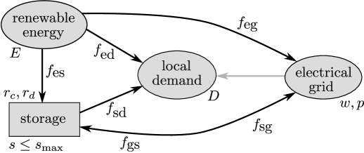
Figure 1: Flow diagram of a convex energy storage problem.

The SP model (1) of the energy storage problem can be formulated by using the decision variable ${\bm{x}}_{t}\doteq[s_{t}\,\,f_{\textrm{es},t}\,\,f_{\textrm{ed},t}\,\,f_{\textrm{eg},t}\,\,f_{\textrm{sd},t}\,\,f_{\textrm{sg},t}\,\,f_{\textrm{gs},t}]^{\top}\in[0,\infty)^{7}$ and setting ${\bm{\mathcal{Z}}}_{t}\doteq[E_{t+1}\,\,D_{t+1}]^{\top}$. Furthermore, the cost function is defined as

$$c_{t}({\bm{x}}_{t},{\bm{\mathcal{Z}}}_{t})\doteq p_{t}(f_{\textrm{gs},t}-f_{\textrm{ed},t}-f_{\textrm{sd},t})-w_{t}(f_{\textrm{eg},t}+f_{\textrm{sg},t})\,,$$

for all $t=1,\ldots,T$, and the dynamics and control constraints are described by

$$\mathbb{X}_{t+1}({\bm{x}}_{t},{\bm{\mathcal{Z}}}_{t})\doteq\left\{\left[\begin{array}[]{c}s\\ f_{\textrm{es}}\\ f_{\textrm{ed}}\\ f_{\textrm{eg}}\\ f_{\textrm{sd}}\\ f_{\textrm{sg}}\\ f_{\textrm{gs}}\end{array}\right]\,\middle|\,\begin{array}[]{c}s=s_{t}+f_{\textrm{es},t}-f_{\textrm{sd},t}-f_{\textrm{sg},t}+f_{\textrm{gs},t},\\ f_{\textrm{es}},f_{\textrm{ed}},f_{\textrm{eg}},f_{\textrm{sd}},f_{\textrm{sg}},f_{\textrm{gs}}\geq 0,\\ 0\leq s+f_{\textrm{es}}-f_{\textrm{sd}}-f_{\textrm{sg}}+f_{\textrm{gs}}\leq s_{\max},\\ f_{\textrm{es}}+f_{\textrm{gs}}\leq r_{c},\,f_{\textrm{sd}}+f_{\textrm{sg}}\leq r_{d},\\ f_{\textrm{es}}+f_{\textrm{ed}}+f_{\textrm{eg}}\leq E_{t+1},\,f_{\textrm{ed}}+f_{\textrm{sd}}\leq D_{t+1}\end{array}\right\}\,,$$

for all $t=0,\ldots,T-1$. To initialize the system, define ${\bm{x}}_{0}\doteq[s_{0}\,\,0\ldots 0]^{\top}$ and ${\bm{z}}_{0}\doteq[d_{1}\,\,e_{1}]^{\top}$, where $s_{1}=s_{0}\in[0,s_{\max}]$ is the current storage level and $d_{1},e_{1}\geq 0$ are the currently observed demand and energy production, respectively.

To set the parameters of this energy storage optimization problem, we consider a solar energy source, a discounted nightly electricity pricing model (Economy 7 tariff), and planning for a two days horizon on hourly basis ($T\doteq 48$). Retail and expected wholesale price curves, along with the electricity demand and energy production distributions of this model are shown on Figure 2 for the two consecutive sunny days.

Figure 2: Parameters of the energy storage optimization problem. Retail ($p$) and expected wholesale ($w$) price curves, energy demand ($D$) and production ($E$) distributions with mean and standard deviation are shown for two-day long period.

The distributions are truncated normal with support $D\in[0,15]$ and $E\in[0,12]$ for demand and energy production, respectively and the storage has capacity $s_{\max}\doteq 20$ with charge and discharge rates $r_{c}\doteq 4$ and $r_{d}\doteq 10$, respectively. The model is initialized by $s_{0}\doteq 0$, $d_{1}\doteq\mathbb{E}[D_{1}]$, and $e_{1}\doteq\mathbb{E}[E_{1}]$.

To evaluate fADP on this problem, we use the CAP and AMAP convex regression algorithms, and multiple configurations determined by the number of trajectories $n$ generated for training (which is the sample size for the regression tasks as well), and the number of evaluations $m$ used to approximate the cost-to-go functions $J_{t}$ at a single point (7). The result is presented on Figure 3,

Figure 3: Energy storage optimization results for the fADP algorithm using AMAP or CAP as the inner convex regression procedure. Results show the total revenue and the training time in minutes with mean and standard deviation for the number of trajectories $n$ and cost-to-go evaluations $m$.

which also includes a “heuristic” algorithm to provide a baseline. The heuristic uses a fixed policy of immediately selling the solar energy preferrably for demand ($f_{\textrm{ed}}\to\max$, $f_{\textrm{eg}}\geq 0$, $f_{\textrm{es}}=0$), selling from the battery during the day when demand still allows ($f_{\textrm{gs}}=0$, $f_{\textrm{sd}}\geq 0$), charging the battery overnight ($f_{\textrm{gs}}\to\max$, $f_{\textrm{sd}}=0$), and selling everything close to the last stage ($f_{\textrm{gs}}=0$, $f_{\textrm{sd}}\to\max$, $f_{\textrm{sg}}\to\max$). This policy is much better than the optimal policy without storage which scores $3227\pm 6$.

The results of Figure 3 show that fADP using either CAP or AMAP significantly outperforms the heuristic baseline algorithm when the sample size is large enough. The regression algorithms prefer larger sample sizes $n$ to better sample quality $m$, although this significantly increases the computation time for CAP and provides only an insignificant revenue increase compared to AMAP.

5.2 Beer brewery operation

Inspired by Bisschop (2016, Chapter 17), we consider the multi-product assembly problem of operating a beer brewery which makes a decision in every two weeks and plans for about one year ($48$ weeks, $T=24$). The factory has to order ingredients (stratch source, yeast, hops) to produce two types of beers (ale and lager) which have to be fermented (for at least $2$ weeks for ale and $6$ weeks for lager) before selling. The states and actions of this process are illustrated on Figure 4.

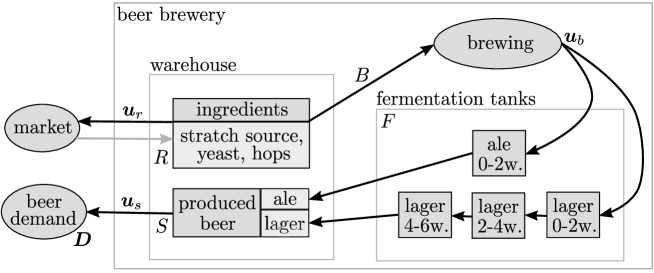
Figure 4: Diagram of the beer brewery problem. The state includes three types of ingredients and two types of bottled beer in the warehouse, and the four fermentation tanks. Actions are formed by ingredient orders ${\bm{u}}_{r}$, brewing amounts ${\bm{u}}_{b}$, and beer sales ${\bm{u}}_{s}$.

The decision variable ${\bm{x}}_{t}$ is a $16$ dimensional vector with the following components:

$${\bm{x}}_{t}\doteq\left[\begin{array}[]{c}\textrm{stratch source in storage}\\ \textrm{yeast in storage}\\ \textrm{hops in storage}\\ \textrm{ale beer fermented for less than 2 weeks}\\ \textrm{produced ale beer}\\ \textrm{lager beer fermented for less than 2 weeks}\\ \textrm{lager beer fermented for 2 to 4 weeks}\\ \textrm{lager beer fermented for 4 to 6 weeks}\\ \textrm{produced lager beer}\\[2.84526pt] \hline\cr\\[-11.38109pt] \textrm{stratch source order}\\ \textrm{yeast order}\\ \textrm{hops order}\\ \textrm{ale beer brewing}\\ \textrm{lager beer brewing}\\ \textrm{ale beer sales}\\ \textrm{lager beer sales}\\ \end{array}\right]\in[0,\infty)^{16}\,.$$

The first $9$ coordinates are state variables, while the last $7$ coordinates represent actions. The cost functions (which may take negative values) are $c_{t}({\bm{x}}_{t},{\bm{\mathcal{Z}}}_{t})\doteq[{\bm{h}}_{t}^{\top}\,{\bm{c}}_{t}^{\top}\,-{\bm{r}}_{t}^{\top}]{\bm{x}}_{t}$, where ${\bm{h}}_{t}\in[0,\infty)^{9}$ is the storage cost, ${\bm{c}}_{t}\in[0,\infty)^{5}$ is the market price of the ingredients with the brewing costs (adjusted by the water price), and ${\bm{r}}_{t}\in[0,\infty)^{2}$ is the selling price of the beers, for stages $t=1,\ldots,T$. The constraint on the dynamics of the system is given by

$$\mathbb{X}_{t+1}({\bm{x}}_{t},{\bm{\mathcal{Z}}}_{t})\doteq\left\{\left[\begin{array}[]{c}F{\bm{x}}_{t}+R{\bm{u}}_{r}+B{\bm{u}}_{b}-S{\bm{u}}_{s}\\ {\bm{u}}_{r}\\ {\bm{u}}_{b}\\ {\bm{u}}_{s}\\ \end{array}\right]\middle|\begin{array}[]{c}{\bm{u}}_{r},{\bm{u}}_{b}\geq{\bm{0}},\,{\bm{u}}_{s}\in[{\bm{0}},{\bm{D}}_{t+1}],\\ F{\bm{x}}_{t}+B{\bm{u}}_{b}-S{\bm{u}}_{s}\geq{\bm{0}},\\ F{\bm{x}}_{t}+R{\bm{u}}_{r}+B{\bm{u}}_{b}\leq{\bm{k}}_{t+1}\\ \end{array}\right\}\,,$$

for all $t=1,\ldots,T-1$, where ${\bm{\mathcal{Z}}}_{t}={\bm{D}}_{t+1}\in[0,\infty)^{2}$ is the beer demand, ${\bm{k}}_{t+1}\in[0,\infty]^{9}$ is the capacity bound, ${\bm{0}}$ denotes a zero vector of appropriate size, and the fermentation matrix $F\in\{0,1\}^{9\times 16}$, the brewing matrix $B\in\mathbb{R}^{9\times 2}$, the storage loading matrix $R\in\{0,1\}^{9\times 3}$ and the selling matrix $S\in\{0,1\}^{9\times 2}$ are defined as

$$F\doteq\left[\begin{array}[]{c|c|c}I_{3}&\lx@intercol\hfil{\bm{0}}_{3\times 13}\hfil\lx@intercol\\ \hline\cr{\bm{0}}_{6\times 3}&\begin{array}[]{cc}\begin{array}[]{cc}0&0\\ 1&1\\ \end{array}&{\bm{0}}_{2\times 4}\\ {\bm{0}}_{4\times 2}&\begin{array}[]{cccc}0&0&0&0\\ 1&0&0&0\\ 0&1&0&0\\ 0&0&1&1\\ \end{array}\end{array}&\,{\bm{0}}_{6\times 7}\end{array}\right]\,,\quad\begin{array}[]{c}B\doteq\left[\begin{array}[]{cc}-{\bm{b}}_{a}&-{\bm{b}}_{l}\\ 1&0\\ 0&0\\ 0&1\\ \hline\cr\lx@intercol\hfil{\bm{0}}_{3\times 2}\hfil\lx@intercol\\ \end{array}\right]\,,\\ \\ R\doteq\left[\begin{array}[]{c}I_{3}\\ {\bm{0}}_{6\times 3}\\ \end{array}\right]\,,\end{array}\quad S\doteq\left[\begin{array}[]{c}{\bm{0}}_{3\times 2}\\ \hline\cr\begin{array}[]{cc}0&0\\ 1&0\\ 0&0\\ 0&0\\ 0&0\\ 0&1\\ \end{array}\end{array}\right]\,,$$

where ${\bm{0}}_{m\times n}$ is a zero matrix of size $m\times n$, and ${\bm{b}}_{a},{\bm{b}}_{l}\in[0,\infty)^{3}$ are the required ingredients for brewing ales and lagers, respectively. To initialize the system, we use ${\bm{x}}_{0}\doteq{\bm{0}}$ and ${\bm{z}}_{0}\doteq{\bm{0}}$.

To test the fADP algorithm on this problem, we set the horizon to $48$ weeks horizon on a fortnight basis ($T\doteq 24$). The demand distributions ${\bm{\mathcal{Z}}}_{t}$ for lager and ale beers are shown on Figure 5

Figure 5: Lager and ale beer demand distributions for the beer brewery optimization problem with mean and standard deviation are shown for a $48$ weeks horizon.

with mean and standard deviation. Both distributions are truncated normal with support $[0.1,12]$. The cost vectors are set to fixed values for all $t=1,\ldots,T$ as ${\bm{h}}_{t}\doteq[1\,\,0.2\,\,0.2\,\,1\,\,2\,\,1\,\,1\,\,1\,\,2]^{\top}$, ${\bm{c}}_{t}\doteq[20\,\,10\,\,5\,\,1\,\,1]^{\top}$, and ${\bm{r}}_{t}\doteq[90\,\,50]^{\top}$. Furthermore, the ingredient requirement vectors for brewing are ${\bm{b}}_{a}\doteq[1\,\,1\,\,1]^{\top}$ and ${\bm{b}}_{l}\doteq[0.5\,\,0.9\,\,0.8]^{\top}$ for ale and lager, respectively, and the capacity vector is ${\bm{k}}\doteq[10\,\,10\,\,10\,\,10\,\,\infty\,\,10\,\,\infty\,\,\infty\,\,\infty]^{\top}$ to ensure the feasibility (relatively complete recourse) requirements, as discussed in Section 4.

Similar to the energy optimization case, color=blue!20!white,]BG: A reasonable heuristic algorithm would be interesting here too. But due to order and fermentation delays, that’s not so simple now. we use the CAP and AMAP estimators for fADP with various trajectory set sizes $n$ and cost-to-go evaluation numbers $m$. As a baseline, we use the optimal solution for the deterministic version of (1) where ${\bm{\mathcal{Z}}}_{t}$ is replaced by its expectation $\mathbb{E}{\bm{\mathcal{Z}}}_{t}$ for all $t=1,\ldots,T$. The results are presented on Figure 6,

Figure 6: Beer brewery optimization results for fADP algorithm using AMAP and CAP convex regression to approximate the convex cost-to-go functions. Results show the revenue with mean and standard deviation, and the training time in minutes for trajectories $n$ and cost-to-go evaluations $m$.

showing that AMAP improves the performance significantly by collecting revenue over 4100 compared to CAP which stays around 3600.

However, the result also shows that the running time of AMAP become significantly larger than CAP. This indicates that larger max-affine models are trained by AMAP compared to CAP to improve the accuracy of the cost-to-go approximations, that increases the computational cost of the LP tasks of (7), and eventually slows down the fADP algorithm significantly.

Finally, notice that using larger trajectory sets $n$ for AMAP provide better performance for low sample levels $nm$, but the improved sample quality with $m=100$ eventually achieves the same using significantly less computational resources. So it seems to be still possible for max-affine estimators to find better tradeoffs between accuracy and model size.

6 Conclusions and future work

In this paper, we considered solving convex SP problems by the combination of an approximate dynamic programming method (fADP) and convex regression techniques. For the latter, we proposed a new state-of-the-art max-affine estimator (AMAP), and combined it with an approximate dynamic programming algorithm to address two benchmark convex SP problems of moderate size.

Clearly, scaling up the fADP algorithm for larger problems would require further improvements. One of these could be using more expressive convex piecewise-linear representations (e.g., sum-max-affine maps), which might compress the LP tasks enough for the current solvers. For this, Hannah and Dunson (2012) considered various ensemble tehniques (bagging, smearing, and random forests) to enhance the performance of the CAP estimator. However, these techniques still seem to construct too large models to increase the accuracy significantly, that makes the vast amount of LP tasks impractical to solve. Maybe, LP algorithms which can more efficiently solve large number of similar LP problems with different right hand sides (e.g., Gassmann and Wallace, 1996) could help with this issue.

But eventually, it would become inevitable to localize cost-to-go approximations to a fraction of the decision space, perhaps by running fADP iteratively alternating between sampling and estimation phases, and exploring at the boundary of the accurately approximated region of cost-to-go functions in order to find and avoid delayed rewards and costs. However, this is left for future work.

Appendix A Auxiliary tools

The following result is a slight generalization of Theorem 5.3 in Rockafellar (1972).

Lemma 1.

Let $\mathbb{X},\mathbb{Y}$ be two convex sets and $f:\mathbb{X}\times\mathbb{Y}$ be a jointly–convex function in its arguments. Additionally, let $C:\mathbb{X}\to 2^{\mathbb{Y}}$ be a set–valued function for which $\textrm{graph}(C)$ is convex. Then $g({\bm{x}})\doteq\inf_{{\bm{y}}\in C({\bm{x}})}f({\bm{x}},{\bm{y}})$ is a convex function.

Proof.

Let ${\bm{x}}_{1},{\bm{x}}_{2}\in\mathbb{X}$, ${\bm{y}}_{1},{\bm{y}}_{2}\in\mathbb{Y}$ and $\lambda\in(0,1)$. As $\textrm{graph}(C)$ is convex,

$${\bm{y}}_{1}\in C({\bm{x}}_{1}),{\bm{y}}_{2}\in C({\bm{x}}_{2})\quad\Rightarrow\quad\lambda{\bm{y}}_{1}+(1-\lambda){\bm{y}}_{2}\in C\big{(}\lambda{\bm{x}}_{1}+(1-\lambda){\bm{x}}_{2}\big{)}\,.$$

Using this with the fact that the infimum on a subset becomes larger, and the joint–convexity of $f$, we get

$$\begin{split}g\big{(}\lambda{\bm{x}}_{1}+(1-\lambda){\bm{x}}_{2}\big{)}&=\inf_{{\bm{z}}\in C(\lambda{\bm{x}}_{1}+(1-\lambda){\bm{x}}_{2})}f\big{(}\lambda{\bm{x}}_{1}+(1-\lambda){\bm{x}}_{2},{\bm{z}}\big{)}\\ &\leq\inf_{{\bm{y}}_{1}\in C({\bm{x}}_{1})}\inf_{{\bm{y}}_{2}\in C({\bm{x}}_{2})}f\big{(}\lambda{\bm{x}}_{1}+(1-\lambda){\bm{x}}_{2},\lambda{\bm{y}}_{1}+(1-\lambda){\bm{y}}_{2}\big{)}\\ &\leq\inf_{{\bm{y}}_{1}\in C({\bm{x}}_{1})}\inf_{{\bm{y}}_{2}\in C({\bm{x}}_{2})}\lambda f({\bm{x}}_{1},{\bm{y}}_{1})+(1-\lambda)f({\bm{x}}_{2},{\bm{y}}_{2})\\ &=\lambda g({\bm{x}}_{1})+(1-\lambda)g({\bm{x}}_{2})\,,\end{split}$$

which proves the convexity of $g$. ∎

References

- Balázs et al. (2015) G. Balázs, A. György, and C. Szepesvári. Near-optimal max-affine estimators for convex regression. In G. Lebanon and S. Vishwanathan, editors, The 18th International Conference on Artificial Intelligence and Statistics (AISTATS), volume 38 of JMLR W&CP, pages 56–64, 2015.
- Bertsekas (2005) D. P. Bertsekas. Dynamic Programming and Optimal Control, Volume I. Athena Scientific, 3rd edition, 2005.
- Birge and Louveaux (2011) J. R. Birge and F. Louveaux. Introduction to Stochastic Programming. Springer, 2011.
- Bisschop (2016) J. Bisschop. AIMMS Optimization Modeling. 2016. http://www.aimms.com.
- Gassmann and Wallace (1996) H. I. Gassmann and S. W. Wallace. Solving linear programs with multiple right-hand sides: Pricing and ordering schemes. Annals of Operation Research, 64:237–259, 1996.
- Golub and Loan (1996) G. H. Golub and C. F. V. Loan. Matrix Computations. The Johns Hopkins University Press, 3rd edition, 1996.
- Hannah and Dunson (2012) L. A. Hannah and D. B. Dunson. Ensemble methods for convex regression with applications to geometric programming based circuit design. In J. Langford and J. Pineau, editors, The 29th International Conference on Machine Learning (ICML), pages 369–376, 2012.
- Hannah and Dunson (2013) L. A. Hannah and D. B. Dunson. Multivariate convex regression with adaptive partitioning. Journal of Machine Learning Research, 14:3261–3294, 2013.
- Hannah et al. (2014) L. A. Hannah, W. B. Powell, and D. B. Dunson. Semiconvex regression for metamodeling-based optimization. SIAM Journal on Optimization, 24(2):573–597, 2014.
- Jiang and Powell (2015) D. R. Jiang and W. B. Powell. An approximate dynamic programming algorithm for monotone value functions. CoRR, 2015. http://arxiv.org/abs/1401.1590v6.
- Lovász (1999) L. Lovász. Hit-and-run mixes fast. Mathematical Programming, 86(3):443–461, 1999.
- Magnani and Boyd (2009) A. Magnani and S. P. Boyd. Convex piecewise-linear fitting. Optimization and Engineering, 10(1):1–17, 2009.
- Mazumder et al. (2015) R. Mazumder, A. Choudhury, G. Iyengar, and B. Sen. A computational framework for multivariate convex regression and its variants. 2015. http://arxiv.org/abs/1509.08165.
- Powell (2011) W. B. Powell. Approximate Dynamic Programming: Solving the Curses of Dimensionality. John Wiley & Sons, 2nd edition, 2011.
- Puterman (1994) M. L. Puterman. Markov Decision Processes: Discrete Stochastic Dynamic Programming. John Wiley & Sons, 1994.
- Rockafellar (1972) R. T. Rockafellar. Convex Analysis. Princeton University Press, 1972.
- Ruszczyński and Shapiro (2003) A. P. Ruszczyński and A. Shapiro. Stochastic Programming. Elsevier, 2003.
- Shapiro et al. (2009) A. Shapiro, D. Dentcheva, and A. Ruszczyński. Lectures on Stochastic Programming, Modeling and Theory. Society for Industrial and Applied Mathematics and the Mathematical Programming Society, 2009.
- Smith (1984) R. L. Smith. Efficient monte carlo procedures for generating points uniformly distributed over bounded regions. Operations Research, 32(6):1296–1308, 1984.
- Sutton (1998) R. S. Sutton. Reinforcement Learning: An Introduction. MIT Press, 1998.
- Szepesvári (2010) C. Szepesvári. Algorithms for Reinforcement Learning: Synthesis Lectures on Artificial Intelligence and Machine Learning. Morgan & Claypool Publishers, 2010.
- Vempala (2005) S. Vempala. Geometric random walk: A survey. Combinatorial and Computational Geometry, 52:573–612, 2005.