Differential equations of electrodiffusion: constant field solutions, uniqueness, and new formulas of Goldman-Hodgkin-Katz type

The equations governing one-dimensional, steady-state electrodiffusion are considered when there are arbitrarily many mobile ionic species present, in any number of valence classes, possibly also with a uniform distribution of fixed charges. Exact constant field solutions and new formulas of Goldman-Hodgkin-Katz type are found. All of these formulas are exact, unlike the usual approximate ones. Corresponding boundary conditions on the ionic concentrations are identified. The question of uniqueness of constant field solutions with such boundary conditions is considered, and is re-posed in terms of an autonomous ordinary differential equation of order $n+1$ for the electric field, where $n$ is the number of valence classes. When there are no fixed charges, the equation can be integrated once to give the non-autonomous equation of order $n$ considered previously in the literature including, in the case $n=2$, the form of Painlevé’s second equation considered first in the context of electrodiffusion by one of us. When $n=1$, the new equation is a form of Liénard’s equation. Uniqueness of the constant field solution is established in this case.

Running title: Differential equations of electrodiffusion

Key Words: electrodiffusion, Goldman-Hodgkin-Katz formulas, liquid junctions, ionic transport, Painlevé II

AMS subject classifications: 82C70, 92B05, 82D15, 34B15, 34B05

1 Introduction

Electrodiffusion — the transport of charged ions by diffusion and migration — plays a central role in a variety of important physical and biological contexts [1, 2, 3]. Ionic species of various valences may be involved, such as Na⁺, K⁺, Cl^-, Ca⁺⁺, SO${}_{4}\,^{--}$, $\dots$ , with various coefficients of diffusion.

The mathematics involved in modeling electrodiffusion is typically nonlinear, making it a nontrivial task to obtain exact solutions or to determine the status of approximations. Of particular interest in the following is the range of validity of so-called ‘constant field approximations’ and associated Goldman-Hodgkin-Katz (GHK) formulas [4, 5], notions that have been widely analyzed and extensively employed since their introduction, especially in studies of liquid junctions associated with biological membranes [6, 8, 9, 10, 7, 11, 12, 13, 14].

An extension of the Nernst-Planck steady-state model [15, 16] incorporates the effect of the electric field that develops within a liquid junction containing ions in solution, with different diffusion coefficients and carrying different charges [17, 18]. The extension involves the application of Gauss’ Law to relate charge density to electric field, together with the imposition of Einstein’s relation between diffusion coefficients and mobilities of the ions. It is the interplay between diffusion of the ions at different rates and the action of the ensuing electric field on the charges, that leads to nonlinearity of the model.

In many cases, the ionic transport can be regarded as one-dimensional, and the junction can be modeled as a slab occupying $0\leq x\leq\delta$. The ionic species in solution can be grouped into $n$ classes with distinct valences $z_{k}$, $k=1,\,2,\,\dots\,,n$, with $m_{k}$ species in the $k$-th valence class. The $z_{k}$ and $m_{k}$ are integers, with $m_{k}$ positive and $z_{k}$ positive or negative. With the concentration of the $r$-th species in the $k$-th valence class denoted by $c_{kr}(x)$, for $k=1,\,2,\,\dots,\,n$ and $r=1,\,2,\,\dots\,,m_{k}$, and with the induced electric field within the junction denoted by $E(x)$, the governing system of coupled first-order ordinary differential equations (ODEs) is

$$\frac{dc_{kr}(x)}{dx}=\frac{z_{k}\,e}{k_{B}\,T}\,E(x)\,c_{kr}(x)+A_{kr}\,,\qquad\qquad$$ (1a)

$$\frac{dE(x)}{dx}=\left(\frac{4\pi e}{\epsilon}\right)\,\left[\sum_{k=1}^{n}z_{k}\,\left(\sum_{r=1}^{m_{k}}c_{kr}(x)\,\right)+Q\,\right]\,,$$ (1b)

for $0<x<\delta$. Here $A_{kr}=-\Phi_{kr}/D_{kr}$, where $\Phi_{kr}$ denotes the steady (constant) flux in the $x$-direction across the junction, of the $r$-th species in the $k$-th valence class, and $D_{kr}$ denotes the diffusion coefficient of that species. Furthermore, $e$ denotes the electronic charge, $k_{B}$ Boltzmann’s constant, $\epsilon$ the electric permittivity, and $T$ the ambient absolute temperature within the solution in the junction.

Equation (1b) allows for the possibility that in addition to the moving ions there may also be fixed (immobile) ions giving rise to a constant and uniform background charge at concentration $Q\,e$. The necessity to allow for fixed charges in naturally occurring liquid junctions has long been recognized [19, 20, 4]. They play a key role in the so-called “glomerular filtration barrier” in the kidney, for example [21].

An important quantity auxiliary to the system of ODEs (1) is the electric current density

$$J=\sum_{k=1}^{n}z_{k}\,e\,\left(\sum_{r=1}^{m_{k}}\Phi_{kr}\,\right)=-\sum_{k=1}^{n}z_{k}\,e\,\left(\sum_{r=1}^{m_{k}}D_{kr}\,A_{kr}\,\right)\,.$$ (2)

When supplemented by a prescribed value for $J$ and suitable prescribed boundary values (BVs) at $x=0$ and $x=\delta$ for the concentrations $c_{kr}(x)$,

$$c_{kr}(0)=c_{kr0}\,,\quad c_{kr}(\delta)=c_{kr\delta}\,,$$ (3)

systems of equations of the form (1) specify the electrical structure of a wide class of liquid junctions in the steady state, including nerve membranes.

These BVs are commonly assumed to be charge-neutral, so that

$$\sum_{k=1}^{n}z_{k}\,\left(\sum_{r=1}^{m_{k}}c_{kr0}\,\right)+Q=0=\sum_{k=1}^{n}z_{k}\,\left(\sum_{r=1}^{m_{k}}c_{kr\delta}\,\right)+Q\,.$$ (4)

An unusual feature of the models described by (1) and (2) is that the ionic fluxes $\Phi_{kr}$, and hence the $A_{kr}$, although constant, are typically not known a priori but are among the unknowns to be determined from the ODEs, the prescribed BVs (3) for the concentrations, and a prescribed value of the current density (2). Thus there are $2(m_{1}+m_{2}+\dots+m_{n})+1$ unknowns (the concentrations, the steady fluxes and the electric field) to be determined from the system of $(m_{1}+m_{2}+\dots+m_{n})+1$ ODEs (1) and the $2(m_{1}+m_{2}+\dots+m_{n})+1$ boundary conditions (BCs) (3), (2). This complicating feature, together with the inherent nonlinearity of the ODEs, has impeded mathematical analysis.

Much of that analysis has focused on the case with two species with valences $+1$ and $-1$, and with $Q=0$, which is appropriate for example to junctions in which Na⁺ (or K⁺) and Cl^- ions move in solution. In such a case, with the additional restriction that one of the fluxes vanishes, it was shown [17] that the concentration corresponding to the vanishing flux satisfies a second order nonlinear equation that can be transformed into the Painlevé II ODE (PII) [22]. Independently, it was shown [18] that in the same model without this restriction, $E(x)$ satisfies another form of PII. These were perhaps the first appearances of PII in physics or biology. This and other aspects of this simple model have been much studied subsequently (see [3, 25, 27, 26, 28, 29, 30, 23, 24] and references therein). Existence of solutions for charge-neutral boundary conditions (BCs) has been established for this model [31, 32], but it is not known if these solutions are unique. Recent analysis [26, 28] has drawn attention to the relevance to this model, of previously-known exact solutions of PII and of Bäcklund transformations [33] of its solutions more generally, leading to the emergent phenomenon of “flux quantization” [29, 30].

Comparatively little mathematical progress has been made in cases with larger $n$ values, in particular on the classical questions of existence and uniqueness of solutions. The emphasis has been on the structure of the $n$-th order non-autonomous ODE satisfied by $E(x)$ alone [35, 34], in models with $Q=0$ and $n\leq 4$, for various values of the $z_{k}$, but with all $m_{k}=1$, and with the fluxes regarded as prescribed constants, rather than as unknowns to be determined as part of a solution.

In what follows, the general model is considered, with any number of valence classes, any number of species in each class, with fixed charges allowed for, and with the constant fluxes regarded as unknowns to be determined as part of any solution.

Exact solutions of (1) are constructed, with constant electric field. The presence of $Q$ in (1b) typically enables a greater richness of such solutions than would otherwise be the case. For example, if all $z_{k}$ have the same sign, it is clear from (1b) that nontrivial solutions with constant field cannot occur unless $Q$ is nonzero, with the opposite sign. In simple cases the exact solutions constructed here are shown to lead to formulas of GHK type, in a way similar to that by which the usual GHK formulas are obtained from approximate solutions with constant electric field. However, there are important differences. The formulas obtained here are exact, and most are new, but they hold under more restrictive BCs than the usual formulas.

The BCs appropriate to these exact constant-field solutions and formulas of GHK type are identified. Existence of solutions is not an issue here, as the solutions are exhibited explicitly, but the question remains as to the uniqueness of these solutions of the BV problem posed by the system of ODEs with these BCs.

A way to approach this question is suggested, by showing first that as a consequence of (1), the field $E(x)$ satisfies an autonomous ODE of order $(n+1)$, one that has not previously been identified in the context of electrodiffusion. When $Q=0$, this ODE can be integrated once, leading to the ODE of order $n$ considered previously in the $Q=0$ case [35, 34]. That known ODE depends explicitly on $x$ and on the constant of integration. The simple two-species model described above, but now for a general value of $Q$, provides an important example; when $Q\neq 0$, the ODE satisfied by $E(x)$ is autonomous of order $3$, and when $Q=0$, this integrates once to give the familiar $x$-dependent ODE of order $2$ that is a form of PII.

The BCs to be satisfied by the field and its derivatives up to order $n$ are identified next. They follow from those found for the system (1) as appropriate for constant field solutions. The uniqueness problem is now reposed in terms of the ODE and BCs for the field, and uniqueness is proved in the case that there is just one valence class, containing any number of species.

2 Dimensionless formulation

It is convenient to introduce a suitable reference concentration $c_{\rm{ref.}}$, for example the value of $Q$ or, if $Q=0$, a typical BV of one of the concentrations. Then dimensionless quantities can be defined as

$${\hat{x}}=x/\delta\,,\quad{\hat{c}}_{kr}({\hat{x}})=c_{k}(x)/c_{\rm{ref.}}\,,\quad{\hat{Q}}=Q/c_{\rm{ref.}}\,,$$

$${\hat{E}}({\hat{x}})=eE(x)\delta/k_{B}T=E(x)/E_{\rm{ref.}}\,,\quad\!\!\!{\rm say},$$

$${\hat{A}}_{kr}=A_{kr}\,\delta/c_{\rm{ref.}}\,,\quad\mu=4\pi e^{2}\delta^{2}c_{\rm{ref.}}/\epsilon k_{B}T\,,$$ (5)

enabling (1) to be rewritten in a more transparent, dimensionless form as

$${\hat{c}}_{kr}\,^{\prime}=z_{k}\,{\hat{E}}\,{\hat{c}}_{kr}+{\hat{A}}_{kr}\,,\qquad\qquad$$ (6a)

$${\hat{E}}\,^{\prime}=\mu\,\left[\sum_{k=1}^{n}z_{k}\,{\hat{c}}_{k}\,+{\hat{Q}}\right]\,,\qquad\qquad$$ (6b)

for $k=1,\,2,\,\dots,\,n$ and $r=1,\,2,\,\dots\,m_{k}$, where

$${\hat{c}}_{k}=\sum_{r=1}^{m_{k}}\,{\hat{c}}_{kr}\,.$$ (7)

It is also convenient to define

$${\hat{A}}_{k}=\sum_{r=1}^{m_{k}}\,{\hat{A}}_{kr}\,,$$ (8)

so that

$${\hat{c}}_{k}\,^{\prime}=z_{k}\,{\hat{E}}\,{\hat{c}}_{k}+{\hat{A}}_{k}\,.$$ (9)

In (6) and (9) the primes denote differentiation with respect to ${\hat{x}}$, and the ODEs are now to hold for $0<{\hat{x}}<1$. The BCs (3) become

$${\hat{c}}_{kr}(0)={\hat{c}}_{kr0}\,,\quad{\hat{c}}_{kr}(1)={\hat{c}}_{kr1}\qquad\qquad\qquad$$ (10a)

$$({\rm and\quad\!\!\!\!so}\quad{\hat{c}}_{k}(0)=\sum_{r=1}^{m_{k}}\,{\hat{c}}_{kr0}={\hat{c}}_{k0}\,,\quad{\hat{c}}_{k}(1)=\sum_{r=1}^{m_{k}}\,{\hat{c}}_{kr1}={\hat{c}}_{k1})\,,$$ (10b)

where ${\hat{c}}_{kr0}$ and ${\hat{c}}_{kr1}$ are positive constants. When charge-neutrality is imposed on the boundaries, (4) becomes

$$\sum_{k=1}^{n}\,\left(\sum_{r=1}^{m_{k}}\,z_{k}\,{\hat{c}}_{kr0}\right)\,+{\hat{Q}}\,\,\,(=\sum_{k=1}^{n}\,z_{k}\,{\hat{c}}_{k0}\,+{\hat{Q}})=0\,,$$

$$\sum_{k=1}^{n}\,\left(\sum_{r=1}^{m_{k}}\,z_{k}\,{\hat{c}}_{kr1}\right)\,+{\hat{Q}}\,\,\,(=\sum_{k=1}^{n}\,z_{k}\,{\hat{c}}_{k1}\,+{\hat{Q}})=0\,.$$ (11)

The expression (2) for the current density can also be written in dimensionless form as

$${\hat{J}}=J/J_{\rm{ref.}}=-\sum_{k=1}^{n}\,z_{k}\,\left(\sum_{r=1}^{m_{k}}{\hat{D}}_{kr}\,{\hat{A}}_{kr}\right)\,,$$

$${\rm{where}}\quad J_{\rm{ref.}}=\left(\frac{e\,c_{\rm{ref.}}\,D_{\rm{ref.}}}{\delta}\right)\quad{\rm{and}}\quad{\hat{D}}_{kr}=D_{kr}/D_{\rm{ref.}}\,,$$ (12)

with $D_{\rm{ref.}}$ a suitable reference diffusion coefficient, say the sum of the $D_{kr}$.

3 Exact constant field solutions and GHK
formulas

The constant $\mu$ defined in (5) is the squared ratio of the junction width $\delta$ to an internal (or bulk) Debye length [7, 24],

$$\mu=\left(\frac{\delta}{\lambda_{\rm{Debye}}}\right)^{2}\,,\quad\lambda_{\rm{Debye}}=\sqrt{\frac{\epsilon k_{B}T}{4\pi e^{2}c_{\rm{ref.}}}}\,.$$ (13)

The structure of a liquid junction may be such that $\mu\ll 1$. Then (6b) reduces to $|{\hat{E}}\,^{\prime}|\ll 1$, implying that the field is approximately constant throughout the junction. (Note that there is then no requirement that the RHS of (6b) should vanish, which would require that charge-neutrality should hold throughout.)

With ${\hat{E}}$ treated as constant, (6a) reduces to a set of uncoupled linear ODEs for the ${\hat{c}}_{kr}({\hat{x}})$, with constant coefficients. These are easily solved using the BCs (10) (compare with (24) below), leading in the case of zero current density to well-known GHK formulas. This is the situation that seems to be assumed in most discussions of those formulas, but the necessity for the condition $\mu\ll 1$ to hold is rarely made explicit [7, 8]. Furthermore, uncertain ionic solubilities in various media lead to uncertainty in the value of $\mu$, and hence in the degree to which the field is approximately constant [8].

A different approach is taken here. Exact constant-field solutions are identified, and used to derive formulas of GHK type. For such solutions, each side of (6b) vanishes, with no restriction on the size of $\mu$. The vanishing of the RHS of (6b) implies that charge-neutrality holds throughout the junction, including at the boundaries, that is to say

$$\sum_{k=1}^{n}z_{k}\,\left(\sum_{r=1}^{m_{k}}\,{\hat{c}}_{kr}({\hat{x}})\right)+{\hat{Q}}\left(=\sum_{k=1}^{n}z_{k}\,{\hat{c}}_{k}({\hat{x}})+{\hat{Q}}\right)=0\,,\quad 0<{\hat{x}}<1\,,$$ (14)

in addition to (11).

3.1 Constant zero field

Turning then to solutions of (6) with ${\hat{E}}({\hat{x}})={{\hat{E}}_{\rm S}}$, some constant, consider firstly ${{\hat{E}}_{\rm S}}=0$. An associated simple solution of the BV problem posed by (6) and (10) can be seen at once to be given by

$${\hat{E}}({\hat{x}})=0\,,\quad{\hat{c}}_{kr}({\hat{x}})={\hat{c}}_{kr0}+({\hat{c}}_{kr1}-{\hat{c}}_{kr0})\,x\,,\quad{\hat{A}}_{kr}={\hat{c}}_{kr1}-{\hat{c}}_{kr0}\,,$$ (15)

provided ${\hat{c}}_{kr0}$ and ${\hat{c}}_{kr1}$ satisfy (11).

For this solution, the current-density is given from (12) and (15) by

$${\hat{J}}=-\sum_{k=1}^{n}\,z_{k}\,\left(\sum_{r=1}^{m_{k}}{\hat{D}}_{kr}\,({\hat{c}}_{kr1}-{\hat{c}}_{kr0})\right)\,,$$ (16)

so (15) is a solution of the BV problem posed by (6), (10), (11) and (16). Even in this simple case, it is not clear for general $n$ and $m_{k}$ if this is the unique solution of that BV problem. Note that when $n=1$ and $m_{1}=1$, (15) collapses to a solution with ${\hat{E}}({\hat{x}})=0$, ${\hat{c}}_{11}({\hat{x}})=-{\hat{Q}}/z_{1}$, ${\hat{A}}_{11}=0$ and ${\hat{J}}=0$.

3.2 Constant nonzero field

Consider next constant-field solutions of (6) with ${{\hat{E}}_{\rm S}}\neq 0$. Now (9) becomes

$${\hat{c}}_{k}\,^{\prime}=z_{k}\,{{\hat{E}}_{\rm S}}\,{\hat{c}}_{k}+{\hat{A}}_{k}\,,$$ (17)

with general solution

$${\hat{c}}_{k}({\hat{x}})=-\frac{{\hat{A}}_{k}}{z_{k}\,{{\hat{E}}_{\rm S}}}+\gamma_{k}\,e^{z_{k}\,{{\hat{E}}_{\rm S}}\,{\hat{x}}}\,,$$ (18)

where the $\gamma_{k}$ are arbitrary constants. Because the exponentials here with different $z_{k}$ are linearly independent, (14) requires that all the $\gamma_{k}$ vanish. Thus ${\hat{c}}_{k}({\hat{x}})$ is constant for each value of $k$,

$${\hat{c}}_{k}({\hat{x}})=-\frac{{\hat{A}}_{k}}{z_{k}\,{{\hat{E}}_{\rm S}}}={\hat{c}}_{k}^{*}\!\!\quad{\rm say},\!\!\quad 0\leq{\hat{x}}\leq 1\,,$$ (19)

and (14) then requires that

$$\sum_{k=1}^{n}z_{k}\,{\hat{c}}_{k}^{*}=-{\hat{Q}}\,.$$ (20)

From (19) it now follows that

$$\sum_{k=1}^{n}{\hat{A}}_{k}={{\hat{E}}_{\rm S}}\,{\hat{Q}}\,,$$ (21)

and that

$$\sum_{r=1}^{m_{k}}\,{\hat{c}}_{kr}({\hat{x}})=\sum_{r=1}^{m_{k}}\,{\hat{c}}_{kr0}=\sum_{r=1}^{m_{k}}\,{\hat{c}}_{kr1}={\hat{c}}_{k}^{*}\,.$$ (22)

For any $k$ value such that $m_{k}=1$, it follows from (19) and (22) that

$${\hat{c}}_{k1}({\hat{x}})={\hat{c}}_{k}^{*}\,,\quad{\hat{A}}_{k1}=-z_{k}\,{\hat{c}}_{k}^{*}\,{{\hat{E}}_{\rm S}}\,,$$ (23)

and for any $k$ value such that $m_{k}>1$, it follows from (6a) and the first two of (10) that

$${\hat{c}}_{kr}({\hat{x}})=-\frac{{\hat{A}}_{kr}}{z_{k}\,{{\hat{E}}_{\rm S}}}+\left({\hat{c}}_{kr0}+\frac{{\hat{A}}_{kr}}{z_{k}\,{{\hat{E}}_{\rm S}}}\right)\,e^{z_{k}\,{{\hat{E}}_{\rm S}}\,{\hat{x}}}\,,$$ (24)

together with the condition

$${\hat{c}}_{kr1}=-\frac{{\hat{A}}_{kr}}{z_{k}\,{{\hat{E}}_{\rm S}}}+\left({\hat{c}}_{kr0}+\frac{{\hat{A}}_{kr}}{z_{k}\,{{\hat{E}}_{\rm S}}}\right)\,e^{z_{k}\,{{\hat{E}}_{\rm S}}}\,,$$ (25)

or equivalently

$${\hat{A}}_{kr}=({\hat{c}}_{kr0}\,e^{z_{k}\,{{\hat{E}}_{\rm S}}}-{\hat{c}}_{kr1})\,\left(\frac{z_{k}\,{{\hat{E}}_{\rm S}}}{1-e^{z_{k}\,{{\hat{E}}_{\rm S}}}}\right)\,.$$ (26)

Note with the help of (21) that (24) is consistent with the global charge-neutrality condition (14) and the condition (22).

Multiplying ${\hat{A}}_{kr}$ by $z_{k}\,{\hat{D}}_{kr}$ using (23) or (26) as appropriate, summing over $k$ and $r$ values, then using (12), leads to a formula expressing ${\hat{J}}$ in terms of ${{\hat{E}}_{\rm S}}$ and the boundary values (10), which in principle determines ${{\hat{E}}_{\rm S}}$ in terms of the BCs.

3.2.1 Special cases

$\bullet\quad{\bf n}$ arbitrary, ${\bf m_{1}=m_{2}=\dots=m_{n}=1}$

Here each ${\hat{A}}_{k1}$ is as in (23), leading from (12) to

$${\hat{J}}=\sum_{k=1}^{n}\,z_{k}^{2}\,{\hat{c}}_{k}^{*}\,{{\hat{E}}_{\rm S}}\,,\quad{\rm so\quad that}\quad{{\hat{E}}_{\rm S}}=\frac{{\hat{J}}}{\sum_{k=1}^{n}\,z_{k}^{2}\,{\hat{c}}_{k}^{*}}\,.$$ (27)

Then (23) gives

$${\hat{c}}_{k1}={\hat{c}}_{k}^{*}\,,\quad{\hat{A}}_{k1}=-\frac{z_{k}\,{\hat{c}}_{k}^{*}\,{\hat{J}}}{\sum_{k=1}^{n}\,z_{k}^{2}\,{\hat{c}}_{k}^{*}}\,,$$ (28)

completing a solution of the BV problem posed by (6) with the BCs (12) and

$${\hat{c}}_{k10}={\hat{c}}_{k11}={\hat{c}}_{k}^{*}\,.$$ (29)

$\bullet\quad{\bf n}$ arbitrary, all ${\bf m_{k}>1}$

Each ${\hat{A}}_{kr}$ is now given by (26), leading to

$${\hat{J}}=-\sum_{k=1}^{n}\,\frac{z_{k}^{2}\,{{\hat{E}}_{\rm S}}}{e^{z_{k}\,{{\hat{E}}_{\rm S}}}-1}\left(\,\sum_{r=1}^{m_{k}}\,{\hat{D}}_{kr}\,\left({\hat{c}}_{kr1}-{\hat{c}}_{kr0}\,e^{z_{k}\,{{\hat{E}}_{\rm S}}}\right)\right)\,.$$ (30)

This transcendental equation cannot be solved explicitly, but determines ${{\hat{E}}_{\rm S}}$ implicitly after ${\hat{J}}$ is prescribed, together with prescribed boundary values (10) for the concentrations, satisfying the constraints (20), (22).

Once ${{\hat{E}}_{\rm S}}$ is determined, if only implicitly, then ${\hat{A}}_{kr}$ is given by (26), and ${\hat{c}}_{kr}({\hat{x}})$ is given by (24), and a solution of (6) with that value for ${\hat{J}}$ and those boundary values is complete.

When ${\hat{J}}=0$, (30) simplifies to

$$\sum_{k=1}^{n}\,\frac{z_{k}^{2}}{e^{z_{k}\,{{\hat{E}}_{\rm S}}}-1}\,\sum_{r=1}^{m_{k}}\,{\hat{D}}_{kr}\,{\hat{c}}_{kr0}\,e^{z_{k}\,{{\hat{E}}_{\rm S}}}=\sum_{k=1}^{n}\,\frac{z_{k}^{2}}{e^{z_{k}\,{{\hat{E}}_{\rm S}}}-1}\,\sum_{r=1}^{m_{k}}\,{\hat{D}}_{kr}\,{\hat{c}}_{kr1}\,.$$ (31)

This is still intractable in general, but can be solved for ${{\hat{E}}_{\rm S}}$ in the following special cases which, though simple mathematically, are nevertheless important for applications.

$\bullet\quad{\bf n=1,\,m_{1}>1,\,{\hat{J}}=0}$

Here (31) simplifies further to

$$e^{z_{1}\,{{\hat{E}}_{\rm S}}}\,\sum_{r=1}^{m_{1}}\,{\hat{D}}_{1r}\,{\hat{c}}_{1r0}=\sum_{r=1}^{m_{1}}\,{\hat{D}}_{1r}\,{\hat{c}}_{1r1}$$ (32)

leading to the formula

$${{\hat{E}}_{\rm S}}=\frac{1}{z_{1}}\,\log\left(\frac{\sum_{r=1}^{m_{1}}\,{\hat{D}}_{1r}\,{\hat{c}}_{1r1}}{\sum_{r=1}^{m_{1}}\,{\hat{D}}_{1r}\,{\hat{c}}_{1r0}}\right)\,.$$ (33)

In terms of the original, dimensional variables, this reads

$$E_{\rm{S}}=\frac{k_{B}T}{z_{1}\,e\delta}\,\log\left(\frac{\sum_{r=1}^{m_{1}}\,D_{1r}\,c_{1r}(\delta)}{\sum_{r=1}^{m_{1}}\,D_{1r}\,c_{1r}(0)}\right)\,,$$ (34)

while the charge-neutrality condition (14) becomes

$$Q+z_{1}\,\sum_{r=1}^{m_{1}}\,c_{1r}(x)=0\,,\quad 0\leq x\leq\delta\,.$$ (35)

With ${{\hat{E}}_{\rm S}}$ determined, explicit formulas for ${\hat{A}}_{1r}$ and ${\hat{c}}_{1r}({\hat{x}})$, and hence for $A_{1r}$ and $c_{1r}(x)$, can now be constructed if desired from (26) and (24) to complete the solution of (6) and hence of (1).

$\bullet\quad{\bf n=2,\,z_{2}=-z_{1},\,m_{1}>1}$ and ${\bf m_{2}>1,\,{\hat{J}}=0}$

Here (31) simplifies to

$$\frac{1}{e^{z_{1}\,{{\hat{E}}_{\rm S}}}-1}\,\sum_{r=1}^{m_{1}}\,{\hat{D}}_{1r}\,\left({\hat{c}}_{1r1}-{\hat{c}}_{1r0}\,e^{z_{1}\,{{\hat{E}}_{\rm S}}}\right)\qquad\qquad\qquad$$

$$=\frac{-1}{e^{-z_{1}\,{{\hat{E}}_{\rm S}}}-1}\,\sum_{r=1}^{m_{2}}\,{\hat{D}}_{2r}\,\left({\hat{c}}_{2r1}-{\hat{c}}_{2r0}\,e^{-z_{1}\,{{\hat{E}}_{\rm S}}}\right)$$ (36)

and hence to

$$\sum_{r=1}^{m_{1}}\,{\hat{D}}_{1r}\,\left({\hat{c}}_{1r1}-{\hat{c}}_{1r0}\,e^{z_{1}\,{{\hat{E}}_{\rm S}}}\right)=\sum_{r=1}^{m_{2}}\,{\hat{D}}_{2r}\,\left({\hat{c}}_{2r1}\,e^{z_{1}\,{{\hat{E}}_{\rm S}}}-{\hat{c}}_{2r0}\right)$$ (37)

and then

$$e^{z_{1}\,{{\hat{E}}_{\rm S}}}\,\left(\sum_{r=1}^{m_{1}}\,{\hat{D}}_{1r}\,{\hat{c}}_{1r0}+\sum_{r=1}^{m_{2}}\,{\hat{D}}_{2r}\,{\hat{c}}_{2r1}\right)=\left(\sum_{r=1}^{m_{1}}\,{\hat{D}}_{1r}\,{\hat{c}}_{1r1}+\sum_{r=1}^{m_{2}}\,{\hat{D}}_{2r}\,{\hat{c}}_{2r0}\right)\,,$$ (38)

so that

$${{\hat{E}}_{\rm S}}=\frac{1}{z_{1}}\,\log\left(\frac{\sum_{r=1}^{m_{1}}\,{\hat{D}}_{1r}\,{\hat{c}}_{1r1}+\sum_{r=1}^{m_{2}}\,{\hat{D}}_{2r}\,{\hat{c}}_{2r0}}{\sum_{r=1}^{m_{1}}\,{\hat{D}}_{1r}\,{\hat{c}}_{1r0}+\sum_{r=1}^{m_{2}}\,{\hat{D}}_{2r}\,{\hat{c}}_{2r1}}\right)$$ (39)

and, in dimensional form,

$$E_{\rm{S}}=\frac{k_{B}T}{z_{1}\,e\delta}\,\log\left(\frac{\sum_{r=1}^{m_{1}}\,D_{1r}\,c_{1r}(\delta)+\sum_{r=1}^{m_{2}}\,D_{2r}\,c_{2r}(0)}{\sum_{r=1}^{m_{1}}\,D_{1r}\,c_{1r}(0)+\sum_{r=1}^{m_{2}}\,D_{2r}\,c_{2r}(\delta)}\right)\,.$$ (40)

Two further cases with ${\hat{J}}=0$ that involve ${\hat{A}}_{kr}$ of the forms in both (23) and (26) are of interest.

$\bullet\quad{\bf n>1}$ and ${\bf m_{1}>1,\,}$ ${\bf m_{2}=m_{3}=\dots=m_{n}=1,\,{\hat{J}}=0}$

Here ${\hat{A}}_{1r}$ is as in (26) while ${\hat{A}}_{kr}$ is as in (23) for $k>1$, leading with ${\hat{J}}=0$ to

$$\frac{z_{1}^{2}}{1-e^{z_{1}\,{{\hat{E}}_{\rm S}}}}\,\sum_{r=1}^{m_{1}}\,{\hat{D}}_{1r}\,\left({\hat{c}}_{1r1}-{\hat{c}}_{1r0}\,e^{z_{1}\,{{\hat{E}}_{\rm S}}}\right)=\sum_{k=2}^{n}\,z_{k}^{2}\,D_{k1}\,{\hat{c}}_{k}^{*}\,,$$ (41)

and hence, in dimensional form, to

$$E_{\rm{S}}=\frac{k_{B}T}{z_{1}\,e\delta}\,\log\left(\frac{\sum_{r=1}^{m_{1}}\,z_{1}^{2}\,D_{1r}\,c_{1r}(\delta)+\sum_{k=2}^{n}\,z_{k}^{2}\,D_{k1}\,c_{k}^{*}}{\sum_{r=1}^{m_{1}}\,z_{1}^{2}\,D_{1r}\,c_{1r}(0)+\sum_{k=2}^{n}\,z_{k}^{2}\,D_{k1}\,c_{k}^{*}}\right)\,,$$ (42)

where $c_{k}(0)=c_{k}(\delta)=c_{k}^{*}$.

$\bullet\quad{\bf n>2,\,}$ ${\bf z_{2}=-z_{1},\,m_{1}>1,\,m_{2}>1,\,m_{3}=m_{4}=\dots=m_{n}=1,\,{\hat{J}}=0}$

Now ${\hat{A}}_{1r}$ and ${\hat{A}}_{2r}$ are as in (26), with opposite values of $z_{k}$, while ${\hat{A}}_{kr}$ is as in (23) for $k>2$. With ${\hat{J}}=0$, this leads to

$$\frac{z_{1}^{2}}{1-e^{z_{1}\,{{\hat{E}}_{\rm S}}}}\,\sum_{r=1}^{m_{1}}\,{\hat{D}}_{1r}\,\left({\hat{c}}_{1r1}-{\hat{c}}_{1r0}\,e^{z_{1}\,{\hat{E}}_{S}}\right)\qquad\qquad\qquad\qquad\qquad\qquad$$

$$+\frac{z_{1}^{2}}{1-e^{-z_{1}\,{\hat{E}}_{S}}}\,\sum_{r=1}^{m_{2}}\,{\hat{D}}_{2r}\,\left({\hat{c}}_{2r1}-{\hat{c}}_{2r0}\,e^{-z_{1}\,{{\hat{E}}_{\rm S}}}\right)+\sum_{k=3}^{n}\,z_{k}^{2}\,{\hat{D}}_{k1}{\hat{c}}_{k}^{*}=0\,,$$ (43)

and hence to

$$E_{\rm{S}}=\frac{k_{B}T}{z_{1}\,e\delta}\,\times\qquad\qquad\qquad\qquad\qquad\qquad\qquad\qquad\qquad$$

$$\log\left(\frac{\sum_{r=1}^{m_{1}}\,z_{1}^{2}\,D_{1r}\,c_{1r}(\delta)+\sum_{r=1}^{m_{2}}\,z_{1}^{2}\,D_{2r}\,c_{2r}(0)+\sum_{k=3}^{n}\,z_{k}^{2}\,D_{k1}\,c_{k}^{*}}{\sum_{r=1}^{m_{1}}\,z_{1}^{2}\,D_{1r}\,c_{1r}(0)+\sum_{r=1}^{m_{2}}\,z_{1}^{2}\,D_{2r}\,c_{2r}(\delta)+\sum_{k=2}^{n}\,z_{k}^{2}\,D_{k1}\,c_{k}^{*}}\right)\,.$$ (44)

While the formulas (27), (34), (42) and (44) appear to be new, (40) has the same form as the original GHK formula [4, 5] for the corresponding set of ionic species. But it must be emphasized that the basis for the derivation given above is different in all these cases, arising not from an approximation dependent upon a very small ratio of the membrane width $\delta$ to the internal Debye length $\lambda_{\rm Debye}$ of (13), but rather from an exact result that is a consequence of more restrictive BCs as in (11) and the possible presence of fixed charges leading to charge-neutrality throughout. This is an important distinction to be borne in mind, even when comparing (40) and the original GHK formula with the same form.

The distinction is illustrated by the following two numerical studies relating to formula (40) for a hypothetical junction containing four ionic species, two with $z=+1$ and two with $z=-1$, taken here to be Chol⁺ (choline), K⁺ (potassium), Cl^- (chlorine) and Prop^- (propionate). The corresponding diffusion coefficients in dimensionless form were calculated as in (12) from experimental values [39], as ${\hat{D}}_{\rm Chol}=0.17$, ${\hat{D}}_{\rm K}=0.33$, ${\hat{D}}_{\rm Cl}=0.34$ and ${\hat{D}}_{\rm Prop}=0.16$. Boundary values of the concentrations, relative to an arbitrary reference concentration $c_{\rm ref.}$, were chosen to be $0.2$ and $2.5$ for choline (at ${\hat{x}}=0$ and ${\hat{x}}=1$, respectively), $2.4$ and $0.1$ for potassium, $0.5$ and $3.4$ for chlorine, and $3.1$ and $0.2$ for propionate. Then the sum of the choline and potassium concentrations is the same at the two faces, as is the sum of the chlorine and propionate concentrations, consistent with the conditions on BVs in (22). The current-density was set to ${\hat{J}}=0$.

Fig. 1 relates to the situation where the junction also contains fixed charges at a positive concentration $Q/c_{\rm{ref.}}=1.0$, so that the charge-neutrality conditions (11) also hold at each boundary face. In this situation all the conditions necessary for the existence of an exact constant-field solution are satisfied, in which case formula (39) and hence (40) holds exactly, as derived above. The BV problem for the system of ODEs (6) in this case was solved using MATLAB [40], leading to the plots in Fig. 1. The electric field was indeed found to be constant, with non-dimensionalised value ${{\hat{E}}_{\rm S}}=-0.58$, which checks with the value given by the formula (39). Corresponding values of the non-dimensionalised ionic fluxes were also obtained in the process, as ${\hat{A}}_{\rm Chol}=3.15$, ${\hat{A}}_{\rm K}=-1.64$, ${\hat{A}}_{\rm Cl}=1.84$, ${\hat{A}}_{\rm Prop}=-3.94$.

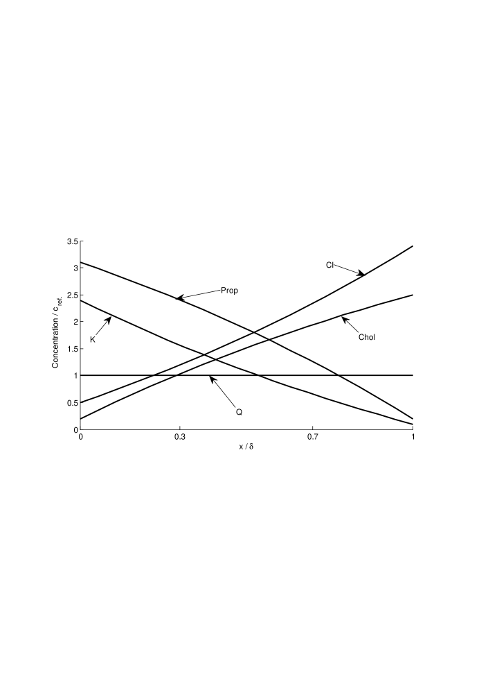
Figure 1: Concentration plots. Fixed charges ensure global charge-neutrality and exact constant field.

Fig. 2 relates to the constant-field approximation for the same system, with the same BCs, and again with ${\hat{J}}=0$, but now with no fixed charges, so that $Q=0$. The plots on the left show the concentration curves for three values of $\mu$, while those on the right show the corresponding graphs of the electric field. They show clearly the nature of the usual approximate approach, with the concentration curves approaching those of Fig.1 as $\mu$ decreases in size, and the electric field approaching, but never equal to the constant value $-0.58$ given by the GHK formula (39), which is not exact in this approximate treatment.

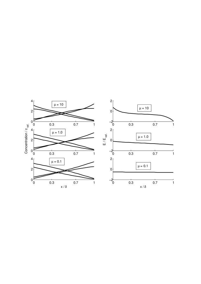
Figure 2: Concentration and electric field plots. No fixed charges, no charge-neutrality, constant-field approximation improves as $\mu$ decreases.

It is remarkable that none of the exact formulas (34), (40), (42) and (44) for ${{\hat{E}}_{\rm S}}$ involves the values of $\mu$ or ${\hat{Q}}$ explicitly. Indeed, the value of $\mu$ has no influence on the value of ${{\hat{E}}_{\rm S}}$ in these formulas (nor on the plots in Fig. 1, for example), in sharp contrast to the usual constant-field approximation, which improves as the value of $\mu$ decreases towards zero. On the other hand, the value of ${\hat{Q}}$ is involved implicitly in the exact formulas through the charge-neutrality conditions (14) and (11). For example, in the cases associated with (34) the condition (35), which is implied in the derivation of (34), can only be satisfied if ${\hat{Q}}$ is nonzero, with opposite sign to $z_{1}$.

The exact formulas (34), (40), (42) and (44) were obtained above from (30), for particular ionic configurations corresponding to special values of $n$ and the $m_{r}$, and with in addition the assumption that ${\hat{J}}=0$. In other cases, (30) and (31) must be solved numerically to obtain ${{\hat{E}}_{\rm S}}$ for given ${\hat{J}}$. This is done most easily by determining ${\hat{J}}$ values directly from (30) for a sufficient density of ${{\hat{E}}_{\rm S}}$ values, and then plotting those ${{\hat{E}}_{\rm S}}$ values against the corresponding ${\hat{J}}$ values. Values of the ${\hat{A}}_{kr}$ at corresponding points can be obtained using (26) and whatever concentration boundary values are prescribed, and then also plotted against ${\hat{J}}$ values. Once ${{\hat{E}}_{\rm S}}$ and the ${\hat{A}}_{kr}$ are effectively determined as functions of ${\hat{J}}$ in this way, ionic concentrations can be determined from (24) and plotted against ${\hat{x}}$.

Fig. 3 shows plots of ${{\hat{E}}_{\rm S}}$, ${\hat{A}}_{11}$ and ${\hat{A}}_{12}$ v. ${\hat{J}}$ obtained in this way from (30) in the case $n=1$, $z_{1}=1$, $m_{1}=2$, with diffusion coefficients taken to be those for K⁺ and Chol⁺ at non-dimensionalised concentrations ${\hat{c}}_{11}({\hat{x}})$ and ${\hat{c}}_{12}({\hat{x}})$ respectively. The BCs were taken to be ${\hat{c}}_{110}=0.25$, ${\hat{c}}_{111}=0.55$, ${\hat{c}}_{120}=0.75$, ${\hat{c}}_{121}=0.45$, with ${\hat{Q}}=-1$ to ensure charge-neutrality. As checks on the numerical calculations, the circled points on the plots in Fig. 3 are at the ‘exact’ values obtained from (33) when ${\hat{J}}=0$.

Figure 3: Plots of ${{\hat{E}}_{\rm S}}$ (solid), ${\hat{A}}_{11}$ (dashed) and ${\hat{A}}_{12}$ (dotted) v. ${\hat{J}}$. Circled points at ${\hat{J}}=0$ obtained independently.

Fig. 4 shows plots of the corresponding concentrations ${\hat{c}}_{11}$ (or K⁺) and ${\hat{c}}_{12}$ (or Chol⁺) v. ${\hat{x}}$ when ${\hat{J}}=1$ (dashed), ${\hat{J}}=0$ (solid) and ${\hat{J}}=-1$ (dotted). Upper curves are for ${\hat{c}}_{11}$, lower curves for ${\hat{c}}_{12}$. For each value of ${\hat{J}}$, charge-neutrality can be seen to hold throughout the junction, with ${\hat{c}}_{11}+{\hat{c}}_{12}+{\hat{Q}}=0$ for all ${\hat{x}}$.

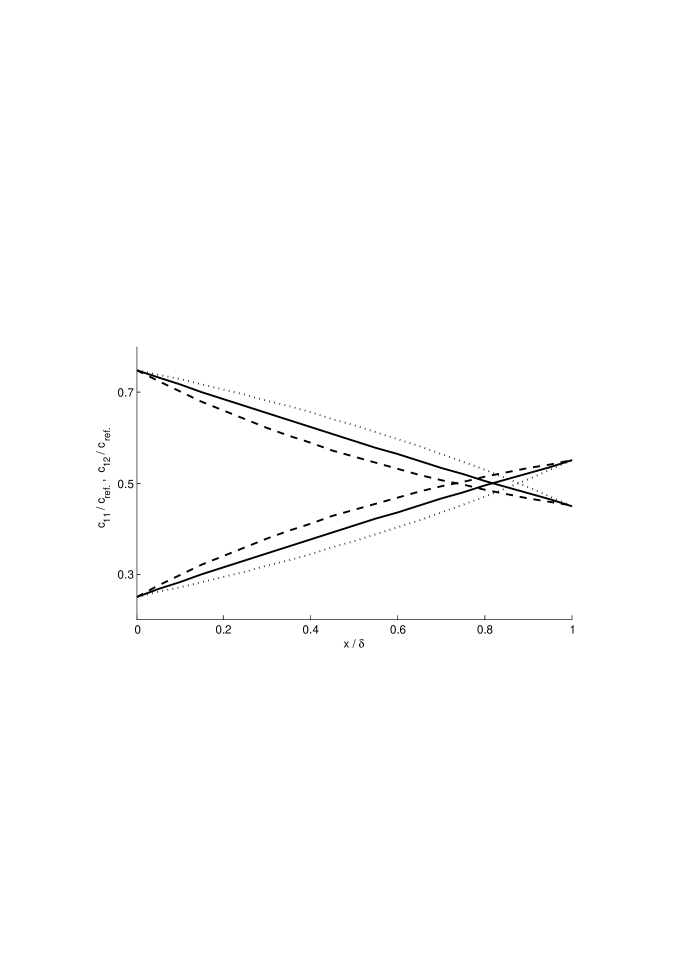
Figure 4: Plots of ${\hat{c}}_{11}$ and ${\hat{c}}_{12}$ v. ${\hat{x}}$, when ${\hat{J}}=1$ (dashed), ${\hat{J}}=0$ (solid), and ${\hat{J}}=-1$ (dotted). In each case ${\hat{Q}}=-1$ and ${\hat{c}}_{11}+{\hat{c}}_{12}+{\hat{Q}}=0$ for all ${\hat{x}}$.

An important mathematical problem that remains is to establish uniqueness of the exact solutions of the corresponding BV problems for the system of ODEs (6). For example, does the formula for ${\hat{E}}({\hat{x}})$ given by (33), together with the consequent formulas for ${\hat{c}}_{kr}({\hat{x}})$ and${\hat{A}}_{kr}$ given from (24) and (26), provide the unique solution of (6) and (10), when the boundary concentration values are also required to have values satisfying (11) and (22)?

One way to approach this problem may be to identify a higher-order ODE satisfied by ${\hat{E}}({\hat{x}})$, together with the BCs on that ODE appropriate to a constant solution, so defining a BV problem for that single ODE. A proof of uniqueness of the solution to that BV problem may be more easily obtained. If and when that is established, the forms of the concentrations and fluxes needed to complete a solution of (6) will follow uniquely in a straightforward way as in the examples above.

In the next section, such an ODE and BCs for ${\hat{E}}({\hat{x}})$ are obtained, for an arbitrary number of ionic species in an arbitrary number of valence classes. This ODE is a generalization of that known [35] when ${\hat{Q}}=0$, where the existence of a first integral of the system (6) leads to an ODE for ${\hat{E}}$ of lower order, and it appears to be a new equation in the context of electrodiffusion.

In the case that there is one valence class containing any number of species, the ODE found is a form of Liénard equation. For this case uniqueness is established.

4 Differential equation for the electric field

Set

$$\sigma_{\nu}({\hat{x}})=\sum_{k=1}^{n}\,z_{k}^{\nu}\,{\hat{c}}_{k}({\hat{x}})\,,\quad\alpha_{\nu}=\sum_{k=1}^{n}\,z_{k}^{\nu}\,{\hat{A}}_{k}\,,$$ (45)

for $\nu=1\,,2\,,\dots\,,n+1$. Now (9) and (45) imply that

$$\sigma_{\nu}\,^{\prime}={\hat{E}}\,\sigma_{\nu+1}+\alpha_{\nu}\,,$$ (46)

and (6b) and (46) then imply by successive differentiations that

$$\sigma_{1}=(1/\mu){\hat{E}}\,^{\prime}-{\hat{Q}}=T_{1}\,,\quad{\rm say}\,,$$

$$\sigma_{2}=\frac{T_{1}\,^{\prime}-\alpha_{1}}{{\hat{E}}}=T_{2}\,,\quad{\rm say}\,,$$ (47)

and in general

$$\sigma_{\nu+1}=\frac{T_{\nu}\,^{\prime}-\alpha_{\nu}}{{\hat{E}}}=T_{\nu+1}\,,\quad{\rm say}\,,$$ (48)

for $\nu=1\,,2\,,\dots\,,n$.

But

$$\sigma_{n+1}\equiv\sigma_{n}\,\sum_{k}\,z_{k}-\sigma_{n-1}\,\sum_{k,\,l}\,^{\prime}\,z_{k}\,z_{l}+\sigma_{n-2}\,\sum_{k,\,l,\,m}\,^{\prime}z_{k}\,z_{l}\,z_{m}-$$

$$\cdots+(-1)^{n-1}\sigma_{1}\,z_{1}\,z_{2}\,\dots\,z_{n}\,,$$ (49)

where $\sum_{k,\,l}\,^{\prime}$ means sum over all distinct unordered pairs of values $k$ and $l$, and so on. It follows that

$$T_{n+1}=T_{n}\,\sum_{k}\,z_{k}-T_{n-1}\,\sum_{k,\,l}\,^{\prime}\,z_{k}\,z_{l}+T_{n-2}\,\sum_{k,\,l,\,m}\,^{\prime}z_{k}\,z_{l}\,z_{m}-$$

$$\cdots+(-1)^{n-1}T_{1}\,z_{1}\,z_{2}\,\dots\,z_{n}\,,$$ (50)

or equivalently, from (47) and (48),

$$T_{n}\,^{\prime}-\alpha_{n}=(T_{n-1}\,^{\prime}-\alpha_{n-1})\,\sum_{k}\,z_{k}-(T_{n-2}\,^{\prime}-\alpha_{n-2})\,\sum_{k,\,l}\,^{\prime}\,z_{k}\,z_{l}+$$

$$\cdots+(-1)^{n-2}\,(T_{1}\,^{\prime}-\alpha_{1})\,\sum_{k,\,l,\,\dots,\,m}\,^{\prime}\,z_{k}\,z_{l}\,\dots\,z_{m}$$

$$+(-1)^{n-1}\,{\hat{E}}\,[(1/\mu){\hat{E}}\,^{\prime}-{\hat{Q}}]\,z_{1}\,z_{2}\,\dots\,z_{n}\,.$$ (51)

This is the autonomous ODE of order $(n+1)$ that ${\hat{E}}$ must satisfy. Note that the last summation in (51) is over all distinct unordered $(n-1)$-tuples of values $k,\,l,\,\dots,\,m$. From (47) and (48),

$$T_{1}=(1/\mu)\,{\hat{E}}\,^{\prime}-{\hat{Q}}\,,\quad T_{2}=\frac{1}{{\hat{E}}}\,[(1/\mu)\,{\hat{E}}\,^{\prime\prime}-\alpha_{1}]\,,$$

$$T_{3}=\frac{1}{{\hat{E}}\,^{3}}\,[(1/\mu)\,{\hat{E}}\,{\hat{E}}\,^{\prime\prime\prime}-(1/\mu)\,{\hat{E}}\,^{\prime}\,{\hat{E}}\,^{\prime\prime}+\alpha_{1}\,{\hat{E}}\,^{\prime}-\alpha_{2}\,{\hat{E}}\,^{2}]\,,$$ (52)

so the first two ODEs are given from (50) or (51) by

$${\bf n=1}\,:\quad{\hat{E}}\,^{\prime\prime}-z_{1}\,{\hat{E}}\,{\hat{E}}\,^{\prime}+\mu z_{1}\,({\hat{Q}}\,{\hat{E}}-{\hat{A}}_{1})=0$$

$${\bf n=2}\,:\quad{\hat{E}}\,{\hat{E}}\,^{\prime\prime\prime}-{\hat{E}}\,^{\prime}\,{\hat{E}}\,^{\prime\prime}-(z_{1}+z_{2})\,{\hat{E}}\,^{2}\,{\hat{E}}\,^{\prime\prime}$$

$$\qquad\qquad+z_{1}z_{2}\,{\hat{E}}\,^{3}\,{\hat{E}}\,^{\prime}+\mu\,(z_{1}{\hat{A}}_{1}+z_{2}{\hat{A}}_{2})\,{\hat{E}}\,^{\prime}$$

$$\qquad-\mu\,z_{1}\,z_{2}\,{\hat{Q}}\,{\hat{E}}\,^{3}+\mu\,z_{1}\,z_{2}\,({\hat{A}}_{1}+{\hat{A}}_{2})\,{\hat{E}}\,^{2}=0\,.$$ (53b)

The ODE (53) for $n=1$ is a form of Liénard’s equation [41], but those for higher values of $n$ are not familiar.

In earlier studies [35, 34], use has been made of the first integral of the system (6) that exists when ${\hat{Q}}=0$, namely

$$\sum_{k=1}^{n}\,{\hat{c}}_{k}-{\textstyle\frac{1}{2}}(1/\mu)\,{\hat{E}}\,^{2}-{\hat{x}}\,\sum_{k=1}^{n}\,{\hat{A}}_{k}=B\quad({\rm const.})\,,$$ (54)

to obtain an ODE of order $n$ for ${\hat{E}}$. This known $n$-th order ODE can be obtained here in a different way by noting that when ${\hat{Q}}=0$, (51) can be integrated once to give

$$T_{n}=T_{n-1}\,\sum_{k}\,^{\prime}\,z_{k}-T_{n-2}\,\sum_{k,\,l}\,^{\prime}\,z_{k}\,z_{l}+$$

$$\cdots+{\textstyle\frac{1}{2}}(-1)^{n-1}\,(1/\mu){\hat{E}}\,^{2}\,z_{1}\,z_{2}\,\dots\,z_{n}$$

$$+[\alpha_{n}-\alpha_{n-1}\,\sum_{k}\,^{\prime}\,z_{k}+\alpha_{n-2}\,\sum_{k,\,l}\,^{\prime}\,z_{k}\,z_{l}-$$

$$\dots+(-1)^{n-1}\,\alpha_{1}\,\sum_{k,\,l,\,\dots,\,m}\,^{\prime}\,z_{k}\,z_{l}\dots z_{m}]\,{\hat{x}}+B\,.$$ (55)

Thus when $n=2$ and $z_{1}=-z_{2}=1$, (53b) integrates once to give

$${\hat{E}}\,^{\prime\prime}-{\textstyle\frac{1}{2}}{\hat{E}}\,^{3}-\mu\,[({\hat{A}}_{1}+{\hat{A}}_{2}){\hat{x}}+B]\,{\hat{E}}-\mu({\hat{A}}_{1}-{\hat{A}}_{2})=0\,,$$ (56)

which is the form of PII much discussed in the literature for this case [3, 25, 27, 26, 28, 31, 32, 29, 30] since it was first discovered more than fifty years ago [18].

The BCs associated with the ODEs for (51) can be found as follows. From (45) and (48),

$$T_{\nu}(0)=\sigma_{\nu}(0)=\sum_{k=1}^{n}\,z_{k}^{\nu}\,{\hat{c}}_{k0}\,,\quad T_{\nu}(1)=\sigma_{\nu}(1)=\sum_{k=1}^{n}\,z_{k}^{\nu}\,{\hat{c}}_{k1}\,,$$ (57)

for $\nu=1,\,2,\,\dots,\,n$.

Thus for $\nu=1$,

$$(1/\mu)\,{\hat{E}}\,^{\prime}(0)={\hat{Q}}+\sum_{k=1}^{n}\,z_{k}\,{\hat{c}}_{k0}\,,\quad(1/\mu)\,{\hat{E}}\,^{\prime}(1)={\hat{Q}}+\sum_{k=1}^{n}\,z_{k}\,{\hat{c}}_{k1}\,,$$ (58)

for $\nu=2$,

$$(1/\mu)\,{\hat{E}}\,^{\prime\prime}(0)={\hat{E}}(0)\,\sum_{k=1}^{n}\,z_{k}^{2}\,{\hat{c}}_{k0}+\sum_{k=1}^{n}\,z_{k}\,{\hat{A}}_{k}\,,$$

$$(1/\mu)\,{\hat{E}}\,^{\prime\prime}(1)={\hat{E}}(1)\,\sum_{k=1}^{n}\,z_{k}^{2}\,{\hat{c}}_{k1}+\sum_{k=1}^{n}\,z_{k}\,{\hat{A}}_{k}\,,$$ (59)

and so on. Then for the cases in (53), the BCs are

$${\bf n=1}\, : {\hat{E}}\,^{\prime}(0)=\mu\,(z_{1}\,{\hat{c}}_{10}+{\hat{Q}})\,,\quad{\hat{E}}\,^{\prime}(1)=\mu\,(z_{1}\,c_{11}+{\hat{Q}})$$ (60a)

$${\bf n=2}\, : {\hat{E}}\,^{\prime}(0)=\mu\,(z_{1}\,{\hat{c}}_{10}+z_{2}\,{\hat{c}}_{20}+{\hat{Q}})\,,$$

$${\hat{E}}\,^{\prime}(1)=\mu\,(z_{1}\,{\hat{c}}_{11}+z_{2}\,{\hat{c}}_{21}+{\hat{Q}})\,,$$

$${\hat{E}}\,^{\prime\prime}(0)=\mu\,{\hat{E}}(0)\,(z_{1}^{2}\,{\hat{c}}_{10}+z_{2}^{2}\,{\hat{c}}_{20})+\mu\,(z_{1}\,{\hat{A}}_{1}+z_{2}\,{\hat{A}}_{2})\,,$$

$${\hat{E}}\,^{\prime\prime}(1)=\mu\,{\hat{E}}(1)\,(z_{1}^{2}\,{\hat{c}}_{11}+z_{2}^{2}\,{\hat{c}}_{21})+\mu\,(z_{1}\,{\hat{A}}_{1}+z_{2}\,{\hat{A}}_{2})\,.$$ (60c)

For general $n$ it is common to impose charge-neutrality at the boundaries as in (11), and then the two BCs for $n=1$ in (60a), and the first two BCs for $n=2$ in (60), simplify to

$${\hat{E}}\,^{\prime}(0)=0={\hat{E}}\,^{\prime}(1)\,.$$ (61)

Note that there are $2n$ BCs in (57) although the ODE (51) for ${\hat{E}}$ is only of order $(n+1)$. This reflects the fact that not only ${\hat{E}}$, but also the ${\hat{A}}_{k}$ appearing in the ODE and in the BCs, are unknowns to be determined as part of a solution of the system of equations (6).

This adds significantly to the difficulty of solving the ODE numerically with the BCs (57), even for small values of $n$. For example, in the case $n=2$ with ${\hat{Q}}=0$, and after (51) has been integrated once to give the Painlevé equation (56), a direct numerical attack proves quite difficult [32]. A way of avoiding these difficulties is to solve the first order system defined by (6b) and (9) from which (51) and (57) are derived, after augmenting it with ODEs expressing the constancy of the ${\hat{A}}_{k}$ in order to construct an enlarged system for which the number of BCs matches the number of dependent variables.

To illustrate, consider the case $n=2$ with $z_{1}=-z_{2}=1$, $m_{1}=m_{2}=1$, and the ODE (53b) with BCs (60) and (60c), which follow from the system

$${\hat{c}}_{1}\,^{\prime}({\hat{x}})={\hat{E}}({\hat{x}})\,{\hat{c}}_{1}({\hat{x}})+{\hat{A}}_{1}\,,\quad{\hat{c}}_{2}\,^{\prime}({\hat{x}})=-{\hat{E}}({\hat{x}})\,{\hat{c}}_{2}({\hat{x}})+{\hat{A}}_{2}\,,$$

$${\hat{E}}\,^{\prime}({\hat{x}})=\mu\left({\hat{c}}_{1}({\hat{x}})-{\hat{c}}_{2}({\hat{x}})+{\hat{Q}}\right)\qquad\qquad\qquad$$ (62)

with BCs ${\hat{c}}_{k}(0)={\hat{c}}_{k0}$, ${\hat{c}}_{k}(1)={\hat{c}}_{k1}$, for $k=1\,,2$, together with a prescribed value for ${\hat{J}}=-{\hat{D}}_{1}\,{\hat{A}}_{1}+{\hat{D}}_{2}\,{\hat{A}}_{2}$, making five constraints in total. Note that there are five unknowns to be determined, namely ${\hat{E}}({\hat{x}})$, the two ${\hat{c}}_{k}({\hat{x}})$ and the two constants ${\hat{A}}_{k}$. The suggestion is to replace (62) and the five constraints by the augmented system of five ODEs

$${\hat{c}}_{1}\,^{\prime}({\hat{x}})={\hat{E}}({\hat{x}})\,{\hat{c}}_{1}({\hat{x}})+{\hat{A}}_{1}({\hat{x}})\,,\quad{\hat{c}}_{2}\,^{\prime}({\hat{x}})=-{\hat{E}}({\hat{x}})\,{\hat{c}}_{2}({\hat{x}})+{\hat{A}}_{2}({\hat{x}})\,,$$

$${\hat{E}}\,^{\prime}({\hat{x}})=\mu\left({\hat{c}}_{1}({\hat{x}})-{\hat{c}}_{2}({\hat{x}})+{\hat{Q}}\right)\,,\quad{\hat{A}}_{1}\,^{\prime}({\hat{x}})=0\,,\quad{\hat{A}}_{2}\,^{\prime}({\hat{x}})=0\,,$$ (63)

with five associated BCs

$${\hat{c}}_{1}(0)={\hat{c}}_{10}\,,\quad{\hat{c}}_{1}(1)={\hat{c}}_{11}\,,\quad{\hat{c}}_{2}(0)={\hat{c}}_{20}\,,\quad{\hat{c}}_{2}(1)={\hat{c}}_{21}\,,$$

$$-{\hat{D}}_{1}\,{\hat{A}}_{1}(0)+{\hat{D}}_{2}\,{\hat{A}}_{2}(0)={\hat{J}}\,.\qquad\qquad\qquad$$ (64)

Now the problem is in a standard form that is easily handled by a standard ODE solver [40].

This technique was used to obtain the solution ${\hat{E}}({\hat{x}})$ of (53b), (60) and (60c), together with the associated values of ${\hat{A}}_{1}$ and ${\hat{A}}_{2}$, for a variety of values of ${\hat{Q}}$ , in order to detect any significant differences in behaviour of the solutions between cases with ${\hat{Q}}\neq 0$ and the case ${\hat{Q}}=0$, which integrates once to the Painlevé equation (56). Fig. 5 shows plots of ${\hat{E}}$ v. ${\hat{x}}$, for ${\hat{Q}}=1,\,0.5,\,0,\,-0.5,\,-1$ from top to bottom, in an example with $\mu=0.3$ and ${\hat{J}}=-0.4$. Dimensionless diffusion coefficients were taken to be ${\hat{D}}_{1}=0.4$, ${\hat{D}}_{2}=0.6$ , as appropriate for Na⁺ and Cl^- [39]. Charge-neutral BCs were adopted in each case, with ${\hat{c}}_{10}=1.5={\hat{c}}_{20}-{\hat{Q}}$, ${\hat{c}}_{11}=1.1={\hat{c}}_{21}-{\hat{Q}}$. The corresponding (constant) values of $({\hat{A}}_{1},\,{\hat{A}}_{2})$ obtained were $(-0.18,\,-0.79),\,(-0.14,\,-0.76)$, $(-0.08,\,-0.72),\,(0.01,\,-0.66),\,(0.19,\,-0.57)$, each consistent with the last of (64).

Figure 5: Plots of ${\hat{E}}({\hat{x}})$ v. ${\hat{x}}$ for ${\hat{Q}}=1$ (top), ${\hat{Q}}=0.5$, ${\hat{Q}}=0$, ${\hat{Q}}=-0.5$, down to ${\hat{Q}}=-1$ (bottom).

The plots show no marked difference in character between the cases, and suggest a smooth transition from ${\hat{Q}}\neq 0$ to ${\hat{Q}}=0$. The nature of singularities that can appear in solutions of PII is well-known and widely-documented [22, 42], but no sign of any singularities occurs in numerical studies of (56) on the finite ${\hat{x}}$- interval with charge-neutral BCs [29], and it seems likely that the same is true for (53b) with ${\hat{Q}}\neq 0$. On the other hand, singularities are known to arise for (56) with more general BCs [30], and it would be interesting to examine (53b) both analytically and numerically in such cases, and also possibly on unbounded regions of the ${\hat{x}}$-axis, or even on the complex ${\hat{x}}$-plane, to identify any new behaviours.

It is not clear for example that when ${\hat{Q}}\neq 0$, (53b) still has the Painlevé property, namely that its general solution is free of branch points whose location in the complex plane is dependent on one or more constants of integration. The ODE does not appear explicitly in Chazy’s classification of third order ODEs with this property [43, 44], but it remains possible that it could be reduced to such an equation by suitable changes of variables. It can be said that (53b) is a generalization of PII in the sense that its solutions must depend on the parameter ${\hat{Q}}$ in such a way that, as ${\hat{Q}}\to 0$, they can be expressed in terms of Painlevé transcendents, but no stronger claim can be made without further analysis. Studies of the singularity properties of (53b), and more generally of the equations (51), are beyond the scope of the present work.

5 Liénard ODE and uniqueness of constant field solution

When $n=1$, there is one class containing $m_{1}$ species with valence $z_{1}$. The electric field ${\hat{E}}$ satisfies the Liénard equation (53), and assuming charge-neutrality on the boundaries as in (11), it also satisfies the BCs (61).

It is obvious by inspection that the BV problem defined by (53) and (61) admits a constant solution

$${\hat{E}}({\hat{x}})={\hat{A}}_{1}/{\hat{Q}}={{\hat{E}}_{\rm S}}\,,\!\!\quad{\rm say},$$ (65)

bearing in mind that the constant ${\hat{A}}_{1}$ is as yet undetermined. It follows from (6b) that with ${\hat{E}}$ constant,

$$z_{1}\,{\hat{c}}_{1}({\hat{x}})+{\hat{Q}}=0\,,\quad 0<{\hat{x}}<1\,.$$ (66)

in other words, charge-neutrality holds throughout the membrane, and not only on the boundaries, as was assumed in (11) and hence in (61).

This is a surprise. It is not obvious that the assumption of charge-neutrality at the boundaries should imply charge-neutrality throughout the membrane, and this raises the question of the uniqueness of the constant solution (65) to the problem posed by (53) and (61) (for any particular value of the constant ${\hat{A}}_{1}$ ). Perhaps there are other, non-constant solutions which, according to (6b), would not imply charge-neutrality?

However, (65) is indeed the unique solution of (53) and (61), so that (65) and (66) do both follow from the assumption (10b). This can be seen as follows.

Note firstly that (66) cannot be satisfied unless ${\hat{Q}}$ is nonzero, with opposite sign to $z_{1}$. Assuming this is so, then (53) can be rewritten as

$${\hat{E}}\,^{\prime\prime}({\hat{x}})-z_{1}\,{\hat{E}}({\hat{x}})\,{\hat{E}}\,^{\prime}({\hat{x}})-\alpha^{2}[{\hat{E}}({\hat{x}})-{{\hat{E}}_{\rm S}}]=0\,,$$ (67)

where $\alpha^{2}=-\mu\,{\hat{Q}}\,z_{1}>0$, with ${{\hat{E}}_{\rm S}}$ as in (65). The problem is to show the uniqueness of the solution (65) of this ODE on $0<{\hat{x}}<1$ with the BCs (61). To be precise, by a solution here is meant a function ${\hat{E}}({\hat{x}})$ with smooth second derivative for $0<{\hat{x}}<1$, satisfying (67) on that interval, and also

$${\hat{E}}\,^{\prime}(0+)=0={\hat{E}}\,^{\prime}(1-)\,.$$ (68)

(A) Note firstly that no solution can have a maximum at any ${\hat{x}}_{m}$ with $0<{\hat{x}}_{m}<1$ and with ${\hat{E}}({\hat{x}}_{m})>{{\hat{E}}_{\rm S}}$. For at such a point, ${\hat{E}}\,^{\prime\prime}({\hat{x}}_{m})\leq 0$, ${\hat{E}}\,^{\prime}({\hat{x}}_{m})=0$ and $[{\hat{E}}({\hat{x}}_{m})-{{\hat{E}}_{\rm S}})]>0$, contradicting (67).

Similarly, no solution can have a minimum at any ${\hat{x}}_{m}$ with $0<{\hat{x}}_{m}<1$ and with ${\hat{E}}({\hat{x}}_{m})<{{\hat{E}}_{\rm S}}$.

(B) Now suppose there exists a solution with ${\hat{E}}(0+)={\hat{E}}_{0}>{{\hat{E}}_{\rm S}}$. Then (67) implies that ${\hat{E}}\,^{\prime\prime}(0+)>0$, so that the graph of ${\hat{E}}({\hat{x}})$ is concave upwards at ${\hat{x}}=0+$.

(a) Suppose in addition to (B) that ${\hat{E}}(1-)={\hat{E}}_{1}>{{\hat{E}}_{\rm S}}$. Then the graph of ${\hat{E}}({\hat{x}})$ is also concave upwards at ${\hat{x}}=1-$, and it follows that ${\hat{E}}({\hat{x}})$ must have a maximum at some ${\hat{x}}_{m}$ with $0<{\hat{x}}_{m}<1$ and with ${\hat{E}}({\hat{x}}_{m})>{{\hat{E}}_{\rm S}}$, implying a contradiction by (A).

(b) Suppose instead in addition to (B) that ${\hat{E}}(1-)={\hat{E}}_{1}\leq{{\hat{E}}_{\rm S}}$. Then again it follows that ${\hat{E}}({\hat{x}})$ must have a maximum at some ${\hat{x}}_{m}$ with $0<{\hat{x}}_{m}<1$ and with ${\hat{E}}({\hat{x}}_{m})>{{\hat{E}}_{\rm S}}$, again implying a contradiction by (A).

Thus there is no solution with ${\hat{E}}(0+)={\hat{E}}_{0}>{{\hat{E}}_{\rm S}}$. Similarly, there is no solution with ${\hat{E}}(0+)={\hat{E}}_{0}<{{\hat{E}}_{\rm S}}$.

Then, similarly, there is no solution with ${\hat{E}}(1-)={\hat{E}}_{1}\neq{{\hat{E}}_{\rm S}}$.

(C) Suppose instead of (B) that there exists a solution with ${\hat{E}}(0+)={{\hat{E}}_{\rm S}}={\hat{E}}(1-)$, but with ${\hat{E}}({\hat{x}})\not\equiv{{\hat{E}}_{\rm S}}$. Then either ${\hat{E}}({\hat{x}})>{{\hat{E}}_{\rm S}}$ or ${\hat{E}}({\hat{x}})<{{\hat{E}}_{\rm S}}$ at some points with $0<{\hat{x}}<1$ (or both). In the first case, ${\hat{E}}({\hat{x}})$ must have a maximum at some ${\hat{x}}_{m}$ with $0<{\hat{x}}_{m}<1$ and with ${\hat{E}}({\hat{x}}_{m})>{{\hat{E}}_{\rm S}}$, while in the second case it must have a minimum at some ${\hat{x}}_{m}$ with $0<{\hat{x}}_{m}<1$ and with ${\hat{E}}({\hat{x}}_{m})<{{\hat{E}}_{\rm S}}$. (In the third case, it must have both). In any case there is a contradiction, by (A).

Thus there is no solution of (67) and (68) except for the constant solution (65).

In any attempt to generalize these arguments to cases with $n\geq 2$, more complicated BCs such as those in (60c) have to be considered, involving the unknowns $\alpha_{k}$ as well as the boundary values of the concentrations ${\hat{c}}_{k}$. It is still unclear if such complications can be overcome so that a proof of uniqueness can be found in such cases.

6 Concluding remarks

Goldman-Hodgkin-Katz formulas are extensively used, especially in physiological settings, to obtain estimates of voltage differences across liquid junctions. The electric field in the junction is assumed to be constant, or approximately so, in the derivation of these formulas, which express the field and hence the voltage difference in terms of BVs of ionic concentrations when the current density across the junction vanishes.

A different approach has been taken above, by explicitly allowing for the presence of a uniform distribution of fixed charges, thus allowing a greater richness of exact constant field solutions and corresponding BVs of the concentrations to be determined. Once again formulas of GHK type are obtained in the case of vanishing current density. In one case this takes a similar form to the usual formula, as in (40), in other cases they appear to be new. But in all cases they are exact, and not derived as approximations following from an assumption that the junction width is small compared with the “internal Debye length” as in (13). The price paid to obtain exactness is that the formulas now hold only for the particular BVs of the concentrations.

The importance of the mathematics of electrodiffusion stems from its numerous significant applications in the physical and biological sciences. The models involved are nonlinear, and the classical questions of existence and uniqueness of solutions have barely been considered in the literature. It is entirely reasonable to suppose, on the basis of numerical experiments, that unique solutions exist for two-point BV problems for the system of coupled ODEs (1) with prescribed current density (2) and BCs (3), when these BCs are charge-neutral. Apart from the explicit appearance of exact constant field solutions as described above, however, existence has been proved more generally only in the case $n=2$, $m_{1}=m_{2}=1$, $z_{1}=-z_{2}=1$ and $Q=0$, and uniqueness not even then. The proof given above of uniqueness of exact constant field solutions in the case $n=1$, $m_{1}$ arbitrary, $Q\neq 0$ is a modest step towards remedying this deficiency, but the uniqueness problem remains unsolved even for exact constant field solutions, when $n>1$.

References

- [1] Teorell, T. Prog. Biophys. Biophysical Chem. 3, 305–369 (1953).
- [2] Schwartz, T.L., in Adelman, W.J. (ed.) Biophysics and Physiology of Excitable Membranes (Van Nostrand-Reinhold, Princeton, 1971).
- [3] Rubinstein, I. Electro-Diffusion of Ions (SIAM, Philadelphia, 1990).
- [4] Goldman, D.E. J. Gen. Physiol. 27, 37–60 (1943).
- [5] Hodgkin, A.L. and Katz, B. J. Physiol. 108, 37–77 (1949).
- [6] Bass, L. and Moore, W.J. Nature 214, 393–394 (1967).
- [7] Agin, D. J. Theoret. Biol 22, 533–534 (1969).
- [8] Moore, W.J. Physical Chemistry. 4th Edition. (Prentice-Hall, New York, 1972), pp. 546-553.
- [9] Zelman, D.A. J. Theoret. Biol. 18, 396–398 (1968).
- [10] Friedman, M.H. J. Theoret. Biol. 25, 502–504 (1969).
- [11] Zelman, D.A. J. Theoret. Biol. 37, 373–383 (1972).
- [12] Arndt, R.A., Bond, J.D. and Roper, L.D. Biophys. J. 10, 1149–1153 (1970).
- [13] Jacquez, J.A. Math. Biosci. 12, 185–196 (1971).
- [14] Syganow, A. and von Kitzing, E. Biophys. J. 76, 768–781 (1999).
- [15] Nernst, W. Z. Phys. Chem. 2, 613–637 (1888).
- [16] Planck, M. Ann. Phys. Chem. 39, 161–186 (1890).
- [17] Grafov, B.M. and Chernenko, A.A. Dokl. Akad. NAUK SSSR 146, 135–138 (1962).
- [18] Bass, L. Trans. Faraday Soc. 60, 1656–1663 (1964).
- [19] Meyer, K.H. and Sievers, J.F. Helv. Chim. Acta 19, 649–664 (1936).
- [20] Teorell, T. Trans. Faraday Soc. 33, 1053 (1937).
- [21] Miner, J.H. Kidney International 74, 259–261 (2008).
- [22] Painlevé, P. Bull. Soc. Math. Phys. Fr. 28, 201–261 (1900).
- [23] Bass, L. Trans. Faraday Soc. 60, 1914–1919 (1964).
- [24] MacGillivray, A.D. and Hare, D. J. Theoret. Biol. 25, 113–26 (1969).
- [25] Ben, Y. and Chang, H.C. J. Fluid Mech. 461, 229 -238 (2002).
- [26] Rogers, C., Bassom, A.P. and Schief, W.K. J. Math. Anal. App. 240, 367–381 (1999).
- [27] Zaltzman, B. and Rubinstein, I. J. Fluid Mech. 579, 173–226 (2007).
- [28] Bass, L., Nimmo, J.J.C., Roger, C. and Schief, W.K. Proc. Roy. Soc.(London) A 466, 2117–2136 (2010).
- [29] Bracken, A.J., Bass, L. and Rogers, C. J. Phys. A: Math. Theoret. 45, Art. No. 105204 (2012).
- [30] Bass, L. and Bracken, A.J. Rep. Math. Phys. 73, 65–75 (2014).
- [31] Thompson, H.B. J. Math. Anal. Appl. 184, 82–94 (1994).
- [32] Amster, P., Kwong, M.K. and Rogers, C. Nonlinear Anal. Theor. Methods Appl. 74, 2897–2907 (2011).
- [33] Rogers, C. and Shadwick, W.F. Bäcklund Transformations and their Applications (Academic Press, New York, 1982).
- [34] Conte, R., Rogers, C. and Schief, W.K. J. Phys. A: Math. Theoret. 40, F1031–40 (2007).
- [35] Leuchtag, H.R. J. Math. Phys. 22, 1317–1320 (1980).
- [36] Schlögl, R. Zeits. Physik. Chemie 1, 305–339 (1954).
- [37] Sistat, P. and Pourcelly, G. J. Electroanal. Chem. 460, 53–62 (1999).
- [38] Bass, L. Proc. Phys. Soc. 85, 1045–1046 (1965).
- [39] web.med.unsw.edu.au/phbsoft/mobility_ listings.htm
- [40] MATLAB (The MathWorks, 2008), routine bvp4c.
- [41] Liénard, A. Revue Générale de Électricité 23, 901–912; 946–954 (1928).
- [42] Clarkson, P.A. Lec. Notes Math. 1883, 331–411 (2006).
- [43] Chazy, J. Acta Math. 34, 317–355 (1911).
- [44] Cosgrove, C.M. Stud. Appl. Math. 104, 171–228 (2000).