Masses of Open-Flavour Heavy-Light Hybrids from QCD Sum-Rules

Abstract

We use QCD Laplace sum-rules to predict masses of open-flavour heavy-light hybrids where one of the hybrid’s constituent quarks is a charm or bottom and the other is an up, down, or strange. We compute leading-order, diagonal correlation functions of several hybrid interpolating currents, taking into account QCD condensates up to dimension-six, and extract hybrid mass predictions for all $J^{P}\in\{0^{\pm},\,1^{\pm}\}$, as well as explore possible mixing effects with conventional quark-antiquark mesons. Within theoretical uncertainties, our results are consistent with a degeneracy between the heavy-nonstrange and heavy-strange hybrids in all $J^{P}$ channels. We find a similar mass hierarchy of $1^{+}$, $1^{-}$, and $0^{+}$ states (a $1^{+}$ state lighter than essentially degenerate $1^{-}$ and $0^{+}$ states) in both the charm and bottom sectors, and discuss an interpretation for the $0^{-}$ states. If conventional meson mixing is present the effect is an increase in the hybrid mass prediction, and we estimate an upper bound on this effect.

1 Introduction

Hybrids are hypothesized, beyond-the-quark-model hadrons that exhibit explicit quark, antiquark, and gluonic degrees of freedom. They are colour singlets and so should be permissible within quantum chromodynamics (QCD); thus, the question of their existence provides us with a key test of our characterization of confinement. Despite nearly four decades of searching, hybrids have not yet been conclusively identified in experiment. There are, however, a number of noteworthy candidates. For example, the Particle Data Group (PDG) OliveEtAl2014 lists a pair of tentative resonances, the $\pi_{1}(1400)$ and the $\pi_{1}(1600)$, both with exotic $J^{PC}=1^{-+}$, a combination inaccessible to conventional quark-antiquark mesons Narison2009 ; Meyer2015 . There are several non-exotic hybrid prospects as well. For instance, each of the resonances $\phi(2170)$, X(3872), Y(3940), and Y(4260) has been singled out as a possible hybrid or at least as a mixed hadron containing a hybrid component DingYan2007 ; ChenJinKleivSteeleWangXu2013 ; Zhu2005 ; Belle2005 ; BergHarnettKleivSteele2012 ; Ketzer2012 .

Definitively assigning a hybrid interpretation to an observed resonance would be greatly facilitated by agreement between theory and experiment concerning the candidate hybrid’s mass. Previous calculations aimed at predicting hybrid masses have been made using a constituent gluon model HornMandula1978 , the MIT bag model BarnesCloseVironEtAl1983 ; ChanowitzSharpe1983 , and the flux tube model IsgurKokoskiPaton1985 ; ClosePage1995 ; BarnesCloseSwanson1995 as well as through the QCD-based approaches of QCD sum-rules Narison2009 ; BergHarnettKleivSteele2012 ; GovaertsVironGusbinEtAl1983 ; GovaertsVironGusbinEtAl1984 ; LatorreNarisonPascualEtAl1984 ; LatorrePascualNarison1987 ; BalitskyDiakonovYung1986 ; JinKoernerSteele2003 ; Huang2015 ; ChetyrkinNarison2000 ; Zhu097502 ; HarnettKleivSteeleJin2012 ; ChenKleivSteeleEtAl2013 ; QiaoTangHaoLi2012 , lattice QCD PerantonisMichael1990 ; LiuMoirPeardonEtAl2012 ; MoirPeardonRyanEtAl2013 ; Dudek2011 , and Heavy Quark Effective Theory HuangJinZhang2000 . Unfortunately, as of yet, there is little consensus concerning hybrid masses.

To date, closed-flavour (hidden-flavour or quarkonium) hybrids have received more attention than open-flavour hybrids likely because most promising hybrid candidates are closed. Furthermore, closed-flavour hybrids allow for exotic $J^{PC}$ quantum numbers; open-flavour hybrids, on the other hand, are not eigenstates of C-parity, and so are characterized by non-exotic $J^{P}$ quantum numbers. However, the recent observation of the fully-open-flavour X(5568) containing a heavy (bottom) quark D0Collab2016 ; LHCbCollab2016 may be a precursor to additional open-flavour discoveries that do not have a simple quark-model explanation (e.g., the X(5568) has been studied as a $\bar{b}\bar{d}su$ tetraquark ChenChenLiuSteeleZhu2016 ). Hence, computing masses of open hybrids containing heavy quarks is timely and of phenomenological relevance.

Ground state masses of bottom-charm hybrids were recently computed using QCD sum-rules in ChenSteeleZhu2014 ; therefore, we focus on a QCD sum-rules analysis of open-flavour heavy-light hybrids i.e., hybrids containing one heavy quark (charm or bottom) and one light quark (up, down, or strange).

The seminal application of QCD Laplace sum-rules to open-flavour hybrids was performed by Govaerts, Reinders, and Weyers GovaertsReindersWeyers1985 (hereafter referred to as GRW). Therein, they considered four distinct currents covering $J\in\{0,\,1\}$ in an effort to compute a comprehensive collection of hybrid masses. Their QCD correlator calculations took into account perturbation theory as well as mass-dimension-three (i.e., 3d) quark and 4d gluon condensate contributions. Precisely half of the analyses stabilized and yielded viable mass predictions. However, for all heavy-light hybrids, the ground state hybrid mass was uncomfortably close to the continuum threshold (with a typical separation of roughly $10\,\text{MeV}$), so that even a modest hadron width would result in the resonance essentially merging with the continuum  GovaertsReindersWeyers1985 .

In this article, we extend the work of GRW by including both 5d mixed and 6d gluon condensate contributions in our correlator calculations. As noted in GRW, for open-flavour heavy-light hybrids, condensates involving light quarks could be enhanced by a heavy quark mass allowing for the possibility of a numerically significant contribution to the sum-rules. By this reasoning, the 5d mixed condensate should also be included. As for the 6d gluon condensate, recent sum-rules analyses of closed-flavour heavy hybrids BergHarnettKleivSteele2012 ; HarnettKleivSteeleJin2012 ; ChenKleivSteeleEtAl2013 ; QiaoTangHaoLi2012 have demonstrated that it is important and can have a stabilizing effect on what were, in the pioneering work GovaertsReindersRubinsteinEtAl1985 ; GovaertsReindersFranckenEtAl1987 , unstable analyses. We also consider the possibility that conventional quark-antiquark mesons couple to the hybrid current, and demonstrate that this leads to an increase in the predicted value of the hybrid mass. A methodology is developed to estimate an upper bound on this mass increase in each channel.

This paper is organized as follows: in Section 2, we define the currents that we use to probe open-flavour heavy-light hybrids and compute corresponding correlation functions; in Section 3, we generate QCD sum-rules for each of the correlators; in Section 4, we present our analysis methodology as well as our mass predictions for those channels which stabilized; in Section 5 we consider the effects of mixing; and, in Section 6, we discuss our results and compare them to GRW and to contemporary predictions made using lattice QCD.

2 Currents and Correlators

Following GRW, we define open-flavour heavy-light hybrid interpolating currents

$$j_{\mu}=\frac{g_{s}}{2}\overline{Q}\Gamma^{\rho}\lambda^{a}q\mathcal{G}^{a}_{\mu\rho}$$ (1)

where $g_{s}$ is the strong coupling and $\lambda^{a}$ are the Gell-Mann matrices. The field $Q$ represents a heavy charm or bottom quark with mass $M_{Q}$ whereas $q$ represents a light up, down, or strange quark with mass $m_{q}$. The Dirac matrix $\Gamma^{\rho}$ satisfies

$$\Gamma^{\rho}\in\{\gamma^{\rho},\,\gamma^{\rho}\gamma_{5}\},\\$$ (2)

and the tensor $\mathcal{G}^{a}_{\mu\rho}$ satisfies

$$\mathcal{G}^{a}_{\mu\rho}\in\{G^{a}_{\mu\rho},\,\tilde{G}^{a}_{\mu\rho}\}$$ (3)

where $G^{a}_{\mu\rho}$ is the gluon field strength and

$$\tilde{G}^{a}_{\mu\rho}=\frac{1}{2}\epsilon_{\mu\rho\nu\sigma}G^{a}_{\nu\sigma}$$ (4)

is its dual defined using the totally antisymmetric Levi-Civita symbol $\epsilon_{\mu\rho\nu\sigma}$.

For each of the four currents defined through (1)–(3), we consider a diagonal correlation function

$$\Pi_{\mu\nu}(q) =i\int\mathrm{d}^{4}x\,e^{iq\cdot x}\langle\Omega|\tau j_{\mu}(x)j^{{\dagger}}_{\nu}(0)|\Omega\rangle$$ (5)

$$=\frac{q_{\mu}q_{\nu}}{q^{2}}\Pi^{(0)}(q^{2})+\left(\frac{q_{\mu}q_{\nu}}{q^{2}}-g_{\mu\nu}\right)\Pi^{(1)}(q^{2})\,,$$ (6)

where $\Pi^{(0)}$ probes spin-0 states and $\Pi^{(1)}$ probes spin-1 states. Each of $\Pi^{(0)}$ and $\Pi^{(1)}$ couples to a particular parity value, and, in the case of closed-flavour hybrids, also to a particular C-parity value; however, as noted in Section 1, open-flavour hybrids are not C-parity eigenstates. Regardless, we will refer to $\Pi^{(0)}$ and $\Pi^{(1)}$ using the $J^{PC}$ assignments they would have if we were investigating closed- rather than open-flavour hybrids. But, to stress that the $C$-value cannot be taken literally, we will enclose it in brackets (a notation employed in ChenSteeleZhu2014 ; HilgerKrassnigg ). In Table 1, we provide a breakdown of which currents couple to which $J^{P(C)}$ combinations.

Table 1: The $J^{P(C)}$ combinations probed through different choices of $\Gamma^{\rho}$ (2) and $\mathcal{G}^{a}_{\mu\rho}$ (3).

$\Gamma^{\rho}$	$\mathcal{G}^{a}_{\mu\rho}$	$J^{P(C)}$
$\gamma^{\rho}$	$G^{a}_{\mu\rho}$	$0^{+(+)},\,1^{-(+)}$
$\gamma^{\rho}$	$\tilde{G}^{a}_{\mu\rho}$	$0^{-(+)},\,1^{+(+)}$
$\gamma^{\rho}\gamma_{5}$	$G^{a}_{\mu\rho}$	$0^{-(-)},\,1^{+(-)}$
$\gamma^{\rho}\gamma_{5}$	$\tilde{G}^{a}_{\mu\rho}$	$0^{+(-)},\,1^{-(-)}$

We calculate the correlators (5) within the operator product expansion (OPE) in which perturbation theory is supplemented by a collection of non-perturbative terms, each of which is the product of a perturbatively computed Wilson coefficient and a non-zero vacuum expectation value (VEV) corresponding to a QCD condensate. We include condensates up to 6d:

$$\langle\overline{q}q\rangle=\langle\overline{q}_{i}^{\alpha}q_{i}^{\alpha}\rangle$$ (7)

$$\langle\alpha G^{2}\rangle=\langle\alpha_{s}G^{a}_{\mu\nu}G^{a}_{\mu\nu}\rangle$$ (8)

$$\langle g\overline{q}\sigma Gq\rangle=\langle g_{s}\overline{q}_{i}^{\alpha}\sigma^{\mu\nu}_{ij}\lambda^{a}_{\alpha\beta}G^{a}_{\mu\nu}q_{j}^{\beta}\rangle$$ (9)

$$\langle g^{3}G^{3}\rangle=\langle g_{s}^{3}f^{abc}G^{a}_{\mu\nu}G^{b}_{\nu\rho}G^{c}_{\rho\mu}\rangle\,,$$ (10)

respectively referred to as the 3d quark condensate, the 4d gluon condensate, the 5d mixed condensate, and the 6d gluon condensate. Superscripts on light quark fields are colour indices whereas subscripts are Dirac indices, and $\sigma^{\mu\nu}=\frac{i}{2}[\gamma^{\mu},\gamma^{\nu}]$. The Wilson coefficients (including perturbation theory) are computed to leading-order (LO) in $g_{s}$ using coordinate-space fixed-point gauge techniques (see BaganAhmadyEliasEtAl1994 ; PascualTarrach1984 , for example). Note that LO contributions to (5) associated with 6d quark condensates are $\mathcal{O}(g_{s}^{4})$; our calculation is actually $\mathcal{O}({g_{s}^{3}})$, and so 6d quark condensates have been excluded from (7)–(10). (In Ref. ChenKleivSteeleEtAl2013 the numerical effect of the 6d quark condensates has been shown to be small compared to the 6d gluon condensate). Light quark mass effects are included in perturbation theory through a next-to-leading-order light quark mass expansion, and at leading-order in all other OPE terms. The contributing Feynman diagrams are depicted in Figure 1 where we follow as closely as possible the labeling scheme of LatorrePascualNarison1987 . (Note that there is no Diagram IV in Figure 1 because, in LatorrePascualNarison1987 , Diagram IV corresponds to an OPE contribution stemming from 6d quark condensates that is absent in the open-flavour heavy-light systems.) The $\overline{\rm MS}$-scheme with the $D=4+2\epsilon$ convention is used, and $\mu$ is the corresponding renormalization scale. We use the program TARCER MertigScharf1998 , which implements the recurrence algorithm of Tarasov1996 ; Tarasov1997 , to express each diagram in terms of a small collection of master integrals, all of which are well-known. Following ChanowitzFurmanHinchliffe1979 , we employ a dimensionally regularized $\gamma_{5}$ that satisfies $\gamma_{5}^{2}=1$ and $\{\gamma_{5},\,\gamma^{\mu}\}=0$. Note that the imaginary parts of Diagrams I–III were actually first computed between GovaertsReindersRubinsteinEtAl1985 and GRW; for these three diagrams, we were able to successfully bench-mark our results against that original work.

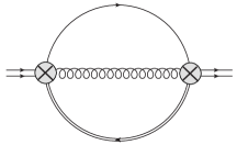
(a) Diagram I (LO perturbation theory)

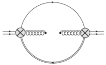
(b) Diagram II (dimension-four)

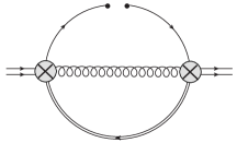
(c) Diagram III (dimension-four)

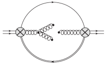
(d) Diagram V (dimension-six)

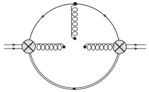
(e) Diagram VI (dimension-six)

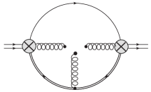
(f) Diagram VI (dimension-six)

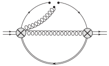
(g) Diagram VII (dimension-five)

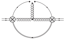
(h) Diagram VIII (dimension-five)

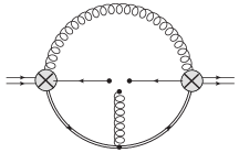
(i) Diagram IX (dimension-five)

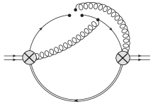
(j) Diagram X (dimension-five)

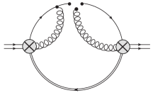
(k) Diagram XI (dimension-five)

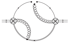
(l) Diagram XII (dimension-five)

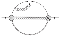
(m) Diagram XIII (dimension-five)

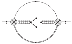
(n) Diagram XIV (dimension-five)

Figure 1: The Feynman diagrams calculated for the correlator (5). Single solid lines correspond to light quark propagators whereas double solid lines correspond to heavy quark propagators.

Diagram XII, a 5d mixed condensate contribution, generates some complications. Focusing on the lower portion of the diagram, we see a heavy quark propagator carrying momentum $q$ multiplied by a divergent, one-loop sub-graph. Correspondingly, Diagram XII contributes to the correlator a non-local divergence proportional to

$$\frac{1}{(q^{2}-M_{Q}^{2})\epsilon}.$$ (11)

Following ChenJinKleivSteeleWangXu2013 , this divergence is eliminated by renormalization of the composite operators (1) which induces mixing with either $\overline{Q}\gamma_{\mu}q$ or $\overline{Q}\gamma_{\mu}\gamma_{5}q$. Specifically, for those operators with $\Gamma^{\rho}=\gamma^{\rho}$ (recall (2)), this mixing results in

$$j_{\mu}\rightarrow j_{\mu}+k\frac{M_{Q}^{2}\alpha_{s}}{\pi\epsilon}\overline{Q}\gamma_{\mu}q$$ (12)

whereas, for those with $\Gamma^{\rho}=\gamma^{\rho}\gamma_{5}$, we have

$$j_{\mu}\rightarrow j_{\mu}+k\frac{M_{Q}^{2}\alpha_{s}}{\pi\epsilon}\overline{Q}\gamma_{\mu}\gamma_{5}q$$ (13)

where $k$ is an as yet undetermined constant emerging from renormalization. For currents that mix according to (12), the VEV under the integral on the right-hand side of (5) gets modified as follows:

$$\langle\Omega|\tau j_{\mu}(x)j^{{\dagger}}_{\nu}(0)|\Omega\rangle\rightarrow\langle\Omega|\tau j_{\mu}(x)j^{{\dagger}}_{\nu}(0)|\Omega\rangle\\ +k\frac{M_{Q}^{2}\alpha_{s}}{\pi\epsilon}\langle\Omega|\tau\overline{Q}(x)\gamma_{\mu}q(x)j_{\nu}^{{\dagger}}(0)|\Omega\rangle+k^{*}\frac{M_{Q}^{2}\alpha_{s}}{\pi\epsilon}\langle\Omega|\tau j_{\mu}(x)\overline{q}(0)\gamma_{\mu}Q(0)|\Omega\rangle$$ (14)

with an analogous expression for operators that mix according to (13). The first term on the right-hand side of (14) corresponds to the diagrams of Figure 1 whereas the last two terms give rise to new, renormalization-induced contributions to the OPE. Almost all of these new contributions are sub-leading in $g_{s}$, however, and so are ignored. The only exceptions are those containing the 5d mixed condensate (9); these give rise to the pair of diagrams depicted in Figure 2. Both of these tree-level diagrams contain a heavy quark propagator with momentum $q$ and are multiplied by a factor of $\frac{1}{\epsilon}$ in (14), precisely what is needed to cancel the non-local divergence (11)

(a)

(b)

Figure 2: Renormalization-induced Feynman diagrams. Square insertion represents the mixing current.

Summing the diagrams from Figures 1 and 2, and then determining the constant $k$ from (12) or (13) such that all non-local divergences are eliminated, we find for either $\Pi^{(0)}$ or $\Pi^{(1)}$ from (6) that

$$\Pi(q^{2})=\frac{M_{Q}^{6}\alpha_{s}}{960\pi^{3}z^{2}}\left[f^{(\text{pert})}_{1}(z)\log(1-z)+f^{(\text{pert})}_{2}(z)\mathrm{Li}_{2}(z)+c^{(\text{pert})}z\right]\\ +\frac{M_{Q}^{5}m_{q}\alpha_{s}}{\pi^{3}z^{2}}\left[f^{(m)}_{1}(z)\log(1-z)+f^{(m)}_{2}(z)\mathrm{Li}_{2}(z)+c^{(m)}z\right]\\ +\frac{M_{Q}^{3}\alpha_{s}\langle\overline{q}q\rangle}{6\pi z^{2}}\left[f^{(qq)}(z)\log(1-z)+c^{(qq)}z\right]\\ +\frac{M_{Q}^{2}\langle\alpha G^{2}\rangle}{144\pi z^{2}}\left[f^{(GG)}(z)\log(1-z)+c^{(GG)}z\right]\\ +\frac{M_{Q}\alpha_{s}\langle g\overline{q}\sigma Gq\rangle}{3456\pi z^{2}}\left[f^{(qGq)}_{1}(z)\log(1-z)+f^{(qGq)}_{2}(z)\frac{z^{2}}{1-z}\log\left(\frac{M_{Q}^{2}}{\mu^{2}}\right)+f^{(qGq)}_{3}(z)\frac{z}{(1-z)}\right]\\ +\frac{\langle g^{3}G^{3}\rangle}{192\pi^{2}z^{2}}\left[f^{(GGG)}(z)\log(1-z)+c^{(GGG)}z\right]\\$$ (15)

where

$$z=\frac{q^{2}}{M_{Q}^{2}}$$ (16)

and where $\mathrm{Li}_{2}(z)$ is the dilogarithm function defined by

$$\mathrm{Li}_{2}(z)=\int_{z}^{\infty}\frac{\mathrm{ln}(1-t)}{t}\mathrm{d}t.$$ (17)

The remaining quantities in (LABEL:correlator_result) are listed in Tables 2–7 for the distinct $J^{P(C)}$ combinations under consideration. Also, in Table 8, we give the values determined for the renormalization parameter $k$. Finally, we note that, for the sake of brevity, we have omitted all polynomials in $z$ corresponding to dispersion-relation subtractions from (LABEL:correlator_result) and Tables 2 to 7. As discussed in Section 3, these subtraction constants do not contribute to the Laplace sum-rules.

Table 2: The polynomials and constants of perturbation theory.

$J$	$f^{(\text{pert})}_{1}(z)$	$f^{(\text{pert})}_{2}(z)$	$c^{(\text{pert})}$
$0$	$-3+30z+20z^{2}-60z^{3}+15z^{4}-2z^{5}$	$-60z^{2}$	-3
$1$	$-1-140z^{2}+100z^{3}+45z^{4}-4z^{5}$	$60z^{2}(1+2z)$	-1

Table 3: The polynomials and constants of the light quark mass correction to perturbation theory.

$J^{P(C)}$	$f^{(m)}_{1}(z)$	$f^{(m)}_{2}(z)$	$c^{(\text{m})}$
$0^{+(+)}$	$3(1-6z+18z^{2}-10z^{3}-3z^{4})$	$-36z^{3}$	3
$0^{-(-)}$	$-3(1-6z+18z^{2}-10z^{3}-3z^{4})$	$36z^{3}$	-3
$0^{-(+)}$	$3(1-6z+18z^{2}-10z^{3}-3z^{4})$	$-36z^{3}$	3
$0^{+(-)}$	$-3(1-6z+18z^{2}-10z^{3}-3z^{4})$	$36z^{3}$	-3
$1^{+(+)}$	$1-6z+18z^{2}-10z^{3}-3z^{4}$	$-12z^{3}$	1
$1^{-(-)}$	$-(1-6z+18z^{2}-10z^{3}-3z^{4})$	$12z^{3}$	-1
$1^{-(+)}$	$1-6z+18z^{2}-10z^{3}-3z^{4}$	$-12z^{3}$	1
$1^{+(-)}$	$-(1-6z+18z^{2}-10z^{3}-3z^{4})$	$12z^{3}$	-1

Table 4: The polynomials and constants of the 3d quark condensate contribution.

$J^{P(C)}$	$f^{(qq)}(z)$	$c^{(qq)}$
$0^{+(+)}$	$-(1-z)^{3}$	-1
$0^{-(-)}$	$(1-z)^{3}$	1
$0^{-(+)}$	$-(1-z)^{3}$	-1
$0^{+(-)}$	$(1-z)^{3}$	1
$1^{+(+)}$	$-\frac{1}{3}(1-z)^{3}$	$-\frac{1}{3}$
$1^{-(-)}$	$\frac{1}{3}(1-z)^{3}$	$\frac{1}{3}$
$1^{-(+)}$	$-\frac{1}{3}(1-z)^{3}$	$-\frac{1}{3}$
$1^{+(-)}$	$\frac{1}{3}(1-z)^{3}$	$\frac{1}{3}$

Table 5: The polynomials and constants of the 4d gluon condensate contribution.

$J^{P(C)}$	$f^{(GG)}(z)$	$c^{(GG)}$
$0^{+(+)}$	$3(1-z)^{2}(1+2z)$	3
$0^{-(-)}$	$3(1-z)^{2}(1+2z)$	3
$0^{-(+)}$	$-3(1-z)^{2}(1+2z)$	-3
$0^{+(-)}$	$-3(1-z)^{2}(1+2z)$	-3
$1^{+(+)}$	$-(1-z)^{2}(1-4z)$	-1
$1^{-(-)}$	$-(1-z)^{2}(1-4z)$	-1
$1^{-(+)}$	$(1-z)^{2}(1-4z)$	1
$1^{+(-)}$	$(1-z)^{2}(1-4z)$	1

Table 6: The polynomials and constants of the 5d mixed condensate contribution.

$J^{P(C)}$	$f^{(qGq)}_{1}(z)$	$f^{(qGq)}_{2}(z)$	$f^{(qGq)}_{3}(z)$
$0^{+(+)}$	$18(1-z)(13+2z)$	$-36(17-z)$	$9(26+27z-21z^{2})$
$0^{-(-)}$	$-18(1-z)(13+2z)$	$36(17-z)$	$-9(26+27z-21z^{2})$
$0^{-(+)}$	$-18(1-z)(27+2z)$	$-36(7+z)$	$-3(162-351z+29z^{2})$
$0^{+(-)}$	$18(1-z)(27+2z)$	$36(7+z)$	$3(162-351z+29z^{2})$
$1^{+(+)}$	$-6(1-z)(27-38z)$	$12(21+19z)$	$-(162+369z+205z^{2})$
$1^{-(-)}$	$6(1-z)(27-38z)$	$-12(21+19z)$	$162+369z+205z^{2}$
$1^{-(+)}$	$6(1-z)(13-38z)$	$12(51-19z)$	$78-999z+569z^{2}$
$1^{+(-)}$	$-6(1-z)(13-38z)$	$-12(51-19z)$	$-(78-999z+569z^{2})$

Table 7: The polynomials and constants of the 6d gluon condensate contribution.

$J^{P(C)}$	$f^{(GGG)}(z)$	$c^{(GGG)}$
$0^{+(+)}$	-3	-3
$0^{-(-)}$	-3	-3
$0^{-(+)}$	3	3
$0^{+(-)}$	3	3
$1^{+(+)}$	$1-2z$	1
$1^{-(-)}$	$1-2z$	1
$1^{-(+)}$	$-(1-2z)$	-1
$1^{+(-)}$	$-(1-2z)$	-1

Table 8: The renormalization parameter $k$ from (12) and (13).

$J^{P(C)}$	$k$
$0^{+(+)}$	$-\frac{2i}{3}$
$0^{-(-)}$	$-\frac{2i}{3}$
$0^{-(+)}$	$-\frac{1}{3}$
$0^{+(-)}$	$-\frac{1}{3}$
$1^{+(+)}$	$-\frac{5}{9}$
$1^{-(-)}$	$-\frac{5}{9}$
$1^{-(+)}$	$-\frac{4i}{9}$
$1^{+(-)}$	$-\frac{4i}{9}$

3 QCD Laplace Sum-Rules

Viewed as a function of Euclidean momentum $Q^{2}=-q^{2}$, each of $\Pi^{(0)}$ and $\Pi^{(1)}$ from (6) satisfies a dispersion relation

$$\Pi(Q^{2})=\frac{Q^{8}}{\pi}\int_{t_{0}}^{\infty}\frac{\mathrm{Im}\Pi(t)}{t^{4}(t+Q^{2})}\,\mathrm{d}t+\cdots,\ Q^{2}>0$$ (18)

where $\cdots$ represents subtractions constants, collectively a third degree polynomial in $Q^{2}$, and $t_{0}$ represents the appropriate physical threshold. The quantity $\Pi$ on the left-hand side of (18) is identified with the OPE result (LABEL:correlator_result) while $\mathrm{Im}\Pi$ on the right-hand side of (18) is the hadronic spectral function. To eliminate the (generally unknown) subtraction constants and enhance the ground state contribution to the integral, the Borel transform

$$\hat{\mathcal{B}}=\lim_{\stackrel{{\scriptstyle N,Q^{2}\rightarrow\infty}}{{\tau=N/Q^{2}}}}\frac{(-Q^{2})^{N}}{\Gamma(N)}\left(\frac{d}{dQ^{2}}\right)^{N}$$ (19)

is applied to (18) weighted by $(-Q^{2})^{k}$ for $k\geq 0$ to yield the $k^{\text{th}}$-order Laplace sum-rule (LSR) ShifmanVainshteinZakharov1979

$$\mathcal{R}_{k}(\tau)=\int_{t_{0}}^{\infty}t^{k}e^{-t\tau}\frac{1}{\pi}\mathrm{Im}\Pi(t)\,\mathrm{d}t,~{}\mathcal{R}_{k}(\tau)=\frac{1}{\tau}\hat{\mathcal{B}}\left\{(-Q^{2})^{k}\Pi(Q^{2})\right\}.$$ (20)

The Borel transform annihilates polynomials in $Q^{2}$ which eliminates dispersion-relation subtraction constants and justifies our omission of polynomials (divergent or not) from (LABEL:correlator_result). The exponential kernel on the right-hand side of (20) suppresses contributions from excited resonances and the continuum relative to the ground state.

In a typical QCD sum-rules analysis, the hadronic spectral function is parametrized using a small number of hadronic quantities, predictions for which are then extracted using a fitting procedure. We employ the “single narrow resonance plus continuum” model ShifmanVainshteinZakharov1979

$$\frac{1}{\pi}\mathrm{Im}\Pi(t)=f_{H}^{2}m_{H}^{8}\delta(t-m_{H}^{2})+\theta(t-s_{0})\frac{1}{\pi}\mathrm{Im}\Pi^{\text{OPE}}(t)$$ (21)

where $m_{H}$ is the ground state resonance mass, $f_{H}$ is its coupling strength, $\theta$ is a Heaviside step function, $s_{0}$ is the continuum threshold and $\mathrm{Im}\Pi^{\text{OPE}}$ is the imaginary part of the QCD expression for $\Pi$ given in (LABEL:correlator_result). Substituting (21) into (20) gives

$$\mathcal{R}_{k}(\tau)=f_{H}^{2}m_{H}^{8+2k}e^{-m_{H}^{2}\tau}+\int_{s_{0}}^{\infty}t^{k}e^{-t\tau}\frac{1}{\pi}\mathrm{Im}\Pi^{\text{OPE}}(t)\mathrm{d}t,$$ (22)

and, defining continuum-subtracted LSRs by

$$\mathcal{R}_{k}(\tau,\,s_{0})=\mathcal{R}_{k}(\tau)-\int_{s_{0}}^{\infty}t^{k}e^{-t\tau}\frac{1}{\pi}\mathrm{Im}\Pi^{\text{OPE}}(t)\mathrm{d}t,$$ (23)

we find, between (22) and (23), the result

$$\mathcal{R}_{k}(\tau,\,s_{0})=f_{H}^{2}m_{H}^{8+2k}e^{-m_{H}^{2}\tau}.$$ (24)

Finally, using (24), we obtain

$$\frac{\mathcal{R}_{1}(\tau,\,s_{0})}{\mathcal{R}_{0}(\tau,\,s_{0})}=m_{H}^{2},$$ (25)

the central equation of our analysis methodology.

To develop an OPE expression for $\mathcal{R}_{k}(\tau,\,s_{0})$, we exploit a relationship between the Borel transform and the inverse Laplace transform $\hat{\mathcal{L}}^{-1}$ ShifmanVainshteinZakharov1979

$$\begin{split}\frac{1}{\tau}\hat{\mathcal{B}}\left\{f(Q^{2})\right\}&=\hat{\mathcal{L}}^{-1}\left\{f(Q^{2})\right\}\\ &=\frac{1}{2\pi i}\int_{c-i\infty}^{c+i\infty}f(Q^{2})e^{Q^{2}\tau}\mathrm{d}Q^{2}\end{split}$$ (26)

where $c$ is chosen such that $f(Q^{2})$ is analytic to the right of the integration contour in the complex $Q^{2}$-plane. Applying definitions (20) and (23) to (LABEL:correlator_result) and using (26), it is straightforward to show that

$$\mathcal{R}_{0}(\tau,\,s_{0})=M_{Q}^{2}\int_{1}^{\frac{s_{0}}{M_{Q}^{2}}}e^{-xM_{Q}^{2}\tau}\frac{1}{\pi}\mathrm{Im}\Pi^{\text{OPE}}(xM_{Q}^{2})\,\mathrm{d}x\\ +\frac{e^{-M_{Q}^{2}\tau}M_{Q}^{3}\alpha_{s}\langle g\overline{q}\sigma Gq\rangle}{108\pi}\left[a\log\left(\frac{M_{Q}^{2}}{\mu^{2}}\right)+b\right]$$ (27)

and

$$\mathcal{R}_{1}(\tau,\,s_{0})=-\frac{d}{d\tau}\mathcal{R}_{0}(\tau,\,s_{0})$$ (28)

where $a,\,b$ are constants given in Table 9 for each $J^{P(C)}$ combination under investigation. Note that the definite integral in (27) can be evaluated exactly; however, the result is rather long and not particularly illuminating, and so is omitted for brevity.

Table 9: The constants $a$ and $b$ from (27).

$J^{P(C)}$	a	b
$0^{+(+)}$	-18	9
$0^{-(-)}$	18	-9
$0^{-(+)}$	9	-15
$0^{+(-)}$	-9	15
$1^{+(+)}$	15	-23
$1^{-(-)}$	-15	23
$1^{-(+)}$	12	-11
$1^{+(-)}$	-12	11

Renormalization-group (RG) improvement NarisondeRafael1981 dictates that the coupling constant and quark masses in (27) be replaced by their (one-loop, $\overline{\text{MS}}$) running counterparts. The running coupling is given by

$$\alpha_{s}(\mu)=\frac{\alpha_{s}(M_{X})}{1+\frac{1}{12\pi}\left(33-2N_{F}\right)\alpha_{s}(M_{X})\log\left(\frac{\mu^{2}}{M_{X}^{2}}\right)}$$ (29)

where $N_{F}$ is the number of active quark flavors and $M_{X}$ is a reference scale for experimental values of $\alpha_{s}$. In addition, the running heavy quark mass can be expressed as

$$M(\mu)=M(\overline{M})\left[\frac{\alpha_{s}(\mu)}{\alpha_{s}(\overline{M})}\right]^{\frac{12}{33-2N_{f}}}$$ (30)

where $\overline{M}$ is defined by $M(\overline{M})=\overline{M}$, and the running light quark mass can be expressed as

$$m(\mu)=m(2~{}\text{GeV})\left[\frac{\alpha_{s}(\mu)}{\alpha_{s}(2~{}\text{GeV})}\right]^{\frac{12}{33-2N_{f}}},$$ (31)

in anticipation of using the Ref. OliveEtAl2014 light-quark mass values at 2 GeV. For charm systems, we use the renormalization scale $\mu=\overline{M}=M_{c}$ while for bottom systems $\mu=\overline{M}=M_{b}$ with PDG values OliveEtAl2014

$$M_{c}=(1.275\pm 0.025)\ \text{GeV}\,,~{}M_{b}=(4.18\pm 0.03)\ \text{GeV}.$$ (32)

We then evaluate $\alpha_{s}$ via (29) within the relevant flavour thresholds using appropriate Ref. OliveEtAl2014 reference values at the $\tau$ and $Z$ masses

$$\alpha_{s}(M_{\tau})=0.330\pm 0.014\,,~{}\alpha_{s}(M_{Z})=0.1185\pm 0.0006.$$ (33)

Lastly, we use the following values for the light quark masses OliveEtAl2014

$$m_{n}(2~{}\text{GeV})=\frac{1}{2}\left[m_{u}(2~{}\text{GeV})+m_{d}(2~{}\text{GeV})\right]=(3.40\pm 0.25)\ \text{MeV}\,,$$ (34)

$$m_{s}(2~{}\text{GeV})=(93.5\pm 2.5)\ \text{MeV}\,.$$ (35)

The QCD predictions (LABEL:correlator_result) have isospin symmetry because $\langle\bar{u}u\rangle=\langle\bar{d}d\rangle=\langle\bar{n}n\rangle$ and the sub-leading effect of nonstrange quark masses is negligible (i.e., we are effectively in the chiral limit for nonstrange systems).

In addition to specifying expressions for the running coupling and quark masses, we must also specify the numerical values of the condensates (7)–(10). Because of the form of (LABEL:correlator_result), for $\langle\overline{q}q\rangle$ we consider the product

$$M\langle\overline{q}q\rangle=\left(\frac{M}{m}\right)\langle m\overline{q}q\rangle$$ (36)

as both $\frac{M}{m}$ and $\langle m\overline{q}q\rangle$ are RG-invariant quantities. From PCAC GMOR1968 (using Ref. Narison2004 conventions), we have

$$\langle m_{n}\overline{n}n\rangle=-\frac{1}{2}f_{\pi}^{2}m_{\pi}^{2}$$ (37)

$$\langle m_{s}\overline{s}s\rangle=-\frac{1}{2}f_{K}^{2}m_{K}^{2}$$ (38)

where PDG values are used for the meson masses OliveEtAl2014 and the decay constants are RosnerStoneVandeRuth2015

$$f_{\pi}=92.2\pm 3.5\ \text{MeV}\ ,\ f_{K}=110.0\pm 4.2\ \text{MeV}.$$ (39)

The quark mass ratios of strange to light and charm to strange quarks are given in OliveEtAl2014 ; however, in order to consider the RG-invariant product (36) for all open-flavor combinations of interest, we must combine results from OliveEtAl2014 with bottom-flavoured ratios obtained on the lattice Chakraborty2015 . The resulting ratios and their errors (treated in quadrature) are

$$\frac{M_{c}}{m_{n}} =\left(\frac{M_{c}}{m_{s}}\right)\left(\frac{m_{s}}{m_{n}}\right)=322.6\pm 13.6, \frac{M_{c}}{m_{s}} =11.73\pm 0.25,$$ (40)

$$\frac{M_{b}}{m_{n}} =\left(\frac{M_{b}}{M_{c}}\right)\left(\frac{M_{c}}{m_{n}}\right)=1460.7\pm 64.0, \frac{M_{b}}{m_{s}} =52.55\pm 1.30.$$ (41)

For the purely gluonic condensates (8) and (10), we use values from LaunerNarisonTarrach1984 ; Narison2010 :

$$\langle\alpha G^{2}\rangle=(0.075\pm 0.020)\ \text{GeV}^{4}$$ (42)

$$\langle g^{3}G^{3}\rangle=\left((8.2\pm 1.0)\ \text{GeV}^{2}\right)\langle\alpha G^{2}\rangle.$$ (43)

The 5d mixed condensate can be related to the 3d quark condensate through LatorreNarisonPascualEtAl1984 ; Narison1988 ; Narison2005 ; Narison2015

$$\frac{\langle g\overline{q}\sigma Gq\rangle}{\langle\overline{q}q\rangle}\equiv M^{2}_{0}=(0.8\pm 0.1)\,\text{GeV}^{2}.$$ (44)

Because we are using (36) to specify the chiral-violating condensates, in the analysis below, the $\langle\overline{q}q\rangle$ effects are subsumed within dimension-four contributions and $\langle g\overline{q}\sigma Gq\rangle$ effects within dimension-six contributions. As noted above, we choose the central value of the renormalization scale $\mu$ to be $M_{c}$ for the charm systems and $M_{b}$ for the bottom systems.

4 Analysis Methodology and Results

In order to extract stable mass predictions from the QCD sum-rule, we require a suitable range of values for our Borel scale ($\tau$) within which our analysis can be considered reliable. Within this range, we perform a fitting (i.e., minimization) procedure to obtain an optimized value of the continuum onset ($s_{0}$) associated with our resulting mass prediction. We determine the bounds of our Borel scale by examining two conditions: the convergence of the OPE, and the pole contribution to the overall mass prediction, mirroring our previous work done in charmonium and bottomonium systems ChenKleivSteeleEtAl2013 . To enforce OPE convergence and obtain an upper-bound on our Borel window ($\tau_{max}$), we require that contributions to the dimension-four condensate be less than one-third that of the perturbative contribution, and the dimension-six gluon condensate contribute less than one-third of the dimension-four condensate contributions. (See Figure 3 for an example.)

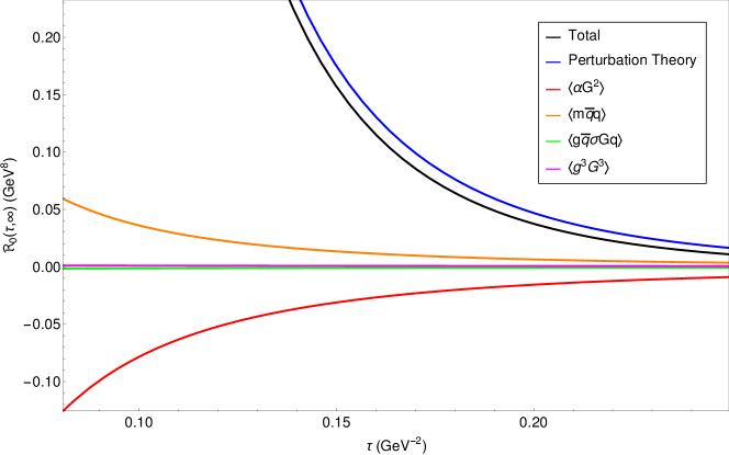
(a)

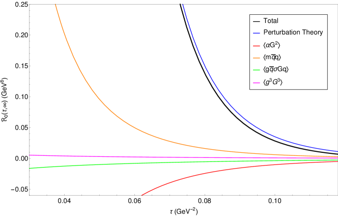
(b)

Figure 3: OPE convergence for $0^{+(+)}$ charm-nonstrange and bottom-nonstrange channels.

To determine a lower bound for our Borel window, we examine the pole contribution defined as

$$\mathrm{PC}\left(s_{0},\tau\right)=\frac{\int_{M_{Q}^{2}}^{s_{0}}e^{-t\tau}\mathrm{Im}\Pi(t)\mathrm{d}t}{\int_{M_{Q}^{2}}^{\infty}e^{-t\tau}\mathrm{Im}\Pi(t)\mathrm{d}t}.$$ (45)

The pole contribution constraint can also be understood as a suppression of excited state contributions. To extract a lower bound for our Borel window ($\tau_{min}$), we must first provide a reasonable estimate of the continuum $s_{0}$ as a seed value for the minimization. To do this, we look for stability in the hadronic mass prediction as a function of $s_{0}$ with variations in $\tau$ (Figure 4).

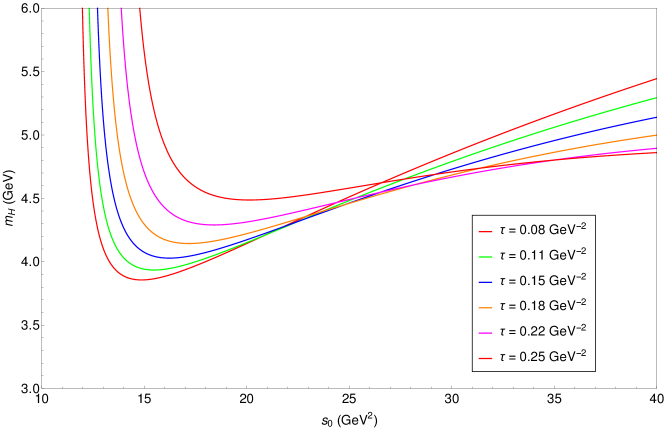
(a)

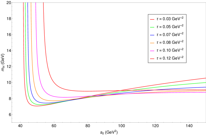
(b)

Figure 4: Plots of hybrid mass $m_{H}$ as a function of continuum threshold $s_{0}$ for various values of the Borel parameter $\tau$ for $0^{+(+)}$ charm-nonstrange and bottom-nonstrange channels.

We optimize the initial $s_{0}$ and $m_{H}$ predictions by minimizing

$$\chi^{2}=\sum_{i=1}^{20}\left(\frac{1}{m_{H}}\sqrt{\frac{\mathcal{R}_{1}(\tau_{i},\,s_{0})}{\mathcal{R}_{0}(\tau_{i},\,s_{0})}}-1\right)^{2},$$ (46)

where we sum over an equally-spaced discretized $\tau$ range inside the Borel window.

Minimizing (46) results in an optimized values for the continuum $s_{0}$. Once $s_{0}$ is found, we may use (45) to determine a lower bound on $\tau$ by requiring a pole contribution of at least $10\%$. Note that this procedure involving (45) should be iterated to ensure that the values of $s_{0}$ and $\tau_{min}$ are self-consistent. Once the hadronic mass prediction has been extracted, we may return to (24) to solve for the hybrid coupling from the $\tau$ critical point of $f_{H}$ using the optimized continuum value and hadronic mass prediction.

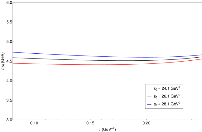
(a)

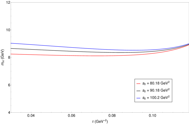
(b)

Figure 5: Plots illustrating the stability of mass predictions for $0^{+(+)}$ charm-nonstrange and bottom-nonstrange channels.

We present results for the Borel window, continuum, and predicted hybrid mass and couplings for open-charm and open-bottom hybrids in Tables 10 through 13, and in Figs. 5 and 6. Channels that do not stabilize have been omitted from the tables. The errors presented encapsulate contributions added in quadrature from the heavy quark masses, quark mass ratios, $\alpha_{s}$ reference values, and the condensate values. We also include estimations of the error due to truncation of the OPE series by comparing mass predictions with and without 6d contributions and due to variations in the $\tau$ window of $10\%$. Uncertainties associated with the renormalization scale follow the methodology established in Ref. Narison_RenormScale2015 which doubled the resulting uncertainty associated with variations in the renormalization scale of $\delta\mu=\pm 0.1\,{\rm GeV}$ (charm systems) and $\delta\mu=\pm 0.5\,{\rm GeV}$ (bottom systems).

Table 10: QCD sum-rules analysis results for ground state charm-nonstrange hybrids.

$J^{PC}$	$\tau_{\min}\ (\text{GeV}^{-2})$	$\tau_{\max}\ (\text{GeV}^{-2})$	$s_{0}\pm\delta s_{0}\ (\text{GeV}^{2})$	$m_{H}\pm\delta m_{H}\ (\text{GeV})$	$f_{H}^{2}\times 10^{6}$
$0^{+(+)}$	0.08	0.25	$26.1\pm 6.0$	$4.55\pm 0.43$	$7.47$
$0^{-(-)}$	0.07	0.17	$31.8\pm 4.2$	$5.07\pm 0.31$	$7.28$
$1^{-(-)}$	0.09	0.29	$24.7\pm 2.5$	$4.40\pm 0.19$	$12.4$
$1^{+(-)}$	0.15	0.35	$14.7\pm 1.6$	$3.39\pm 0.18$	$9.87$

Table 11: QCD sum-rules analysis results for ground state charm-strange hybrids.

$J^{PC}$	$\tau_{\min}\ (\text{GeV}^{-2})$	$\tau_{\max}\ (\text{GeV}^{-2})$	$s_{0}\pm\delta s_{0}\ (\text{GeV}^{2})$	$m_{H}\pm\delta m_{H}\ (\text{GeV})$	$f_{H}^{2}\times 10^{6}$
$0^{+(+)}$	0.08	0.24	$25.2\pm 5.2$	$4.49\pm 0.40$	$7.36$
$0^{-(-)}$	0.07	0.17	$30.4\pm 5.2$	$4.98\pm 0.39$	$2.03$
$1^{-(-)}$	0.10	0.30	$23.1\pm 2.4$	$4.28\pm 0.19$	$11.0$
$1^{+(-)}$	0.18	0.34	$12.5\pm 1.1$	$3.15\pm 0.14$	$8.45$

Table 12: QCD sum-rules analysis results for ground state bottom-nonstrange hybrids.

$J^{PC}$	$\tau_{\min}\ (\text{GeV}^{-2})$	$\tau_{\max}\ (\text{GeV}^{-2})$	$s_{0}\pm\delta s_{0}\ (\text{GeV}^{2})$	$m_{H}\pm\delta m_{H}\ (\text{GeV})$	$f_{H}^{2}\times 10^{6}$
$0^{+(+)}$	0.03	0.12	$92.5\pm 15.6$	$8.57\pm 0.51$	$1.28$
$0^{-(+)}$	0.05	0.09	$59.1\pm 3.9$	$7.01\pm 0.21$	$0.516$
$1^{-(-)}$	0.03	0.10	$94.7\pm 7.5$	$8.74\pm 0.25$	$1.76$
$1^{+(-)}$	0.03	0.14	$86.7\pm 11.1$	$8.26\pm 0.41$	$1.66$

Table 13: QCD sum-rules analysis results for ground state bottom-strange hybrids.

$J^{PC}$	$\tau_{\min}\ (\text{GeV}^{-2})$	$\tau_{\max}\ (\text{GeV}^{-2})$	$s_{0}\pm\delta s_{0}\ (\text{GeV}^{2})$	$m_{H}\pm\delta m_{H}\ (\text{GeV})$	$f_{H}^{2}\times 10^{6}$
$0^{+(+)}$	0.04	0.11	$79.9\pm 13.0$	$8.14\pm 0.49$	$0.817$
$0^{-(+)}$	0.06	0.10	$55.1\pm 4.0$	$6.79\pm 0.22$	$0.434$
$1^{-(-)}$	0.03	0.10	$87.6\pm 9.9$	$8.46\pm 0.32$	$1.24$
$1^{+(-)}$	0.04	0.15	$81.7\pm 15.7$	$8.02\pm 0.59$	$1.39$

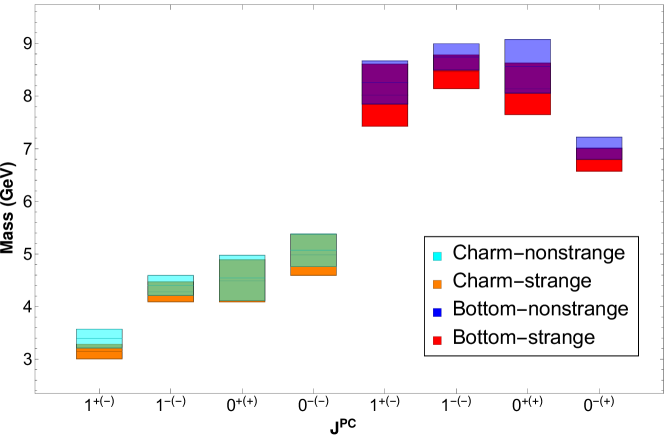
Figure 6: Summary of mass predictions in charm and bottom systems with uncertainties. The overlap between the heavy-nonstrange and heavy-strange predictions is denoted by the green tone in the charm sector and purple in the bottom sector.

Table 14: Charm-Nonstrange Masses from Higher-Weight Sum-Rules (GeV)

$J^{P(C)}$	$\sqrt{\frac{R_{1}}{R_{0}}}$	$\sqrt{\frac{R_{2}}{R_{1}}}$	$\sqrt{\frac{R_{3}}{R_{2}}}$
$0^{+(+)}$	4.54	4.54	4.59
$0^{-(-)}$	5.07	5.07	5.12
$1^{-(-)}$	4.40	4.39	4.45
$1^{+(-)}$	3.39	3.39	3.45

Table 15: Bottom-Nonstrange Masses from Higher-Weight Sum-Rules (GeV)

$J^{P(C)}$	$\sqrt{\frac{R_{1}}{R_{0}}}$	$\sqrt{\frac{R_{2}}{R_{1}}}$	$\sqrt{\frac{R_{3}}{R_{2}}}$
$0^{+(+)}$	8.57	8.52	8.60
$0^{-(+)}$	7.01	7.01	7.06
$1^{-(-)}$	8.74	8.71	8.80
$1^{+(-)}$	8.26	8.20	8.29

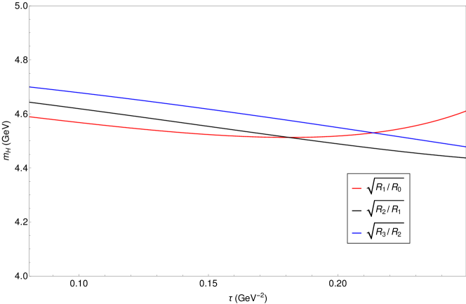
(a)

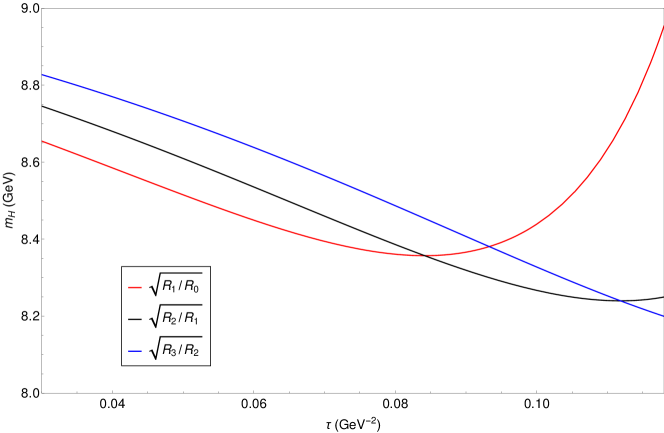
(b)

Figure 7: Plots illustrating higher-weight sum-rule ratios in $0^{+(+)}$ charm-nonstrange and bottom-nonstrange channels.

As a validation of our analysis, we also consider ratios of higher-weight sum-rules which serve as a generalization of (25):

$$\frac{\mathcal{R}_{k+1}(\tau,\,s_{0})}{\mathcal{R}_{k}(\tau,\,s_{0})}=m_{H}^{2}~{}.$$ (47)

In Table 14, Table 15 and Figure 7 we compare the nonstrange sum-rule ratios for $k=0,1,2$. Although the higher-weight ratios have greater sensitivity to the high-energy region of the spectral function (excited states and QCD continuum), the hadronic mass scales emerging from the various weights are remarkably consistent, indicating that the sum-rule window has been well-chosen to emphasize the lightest hybrid state via the pole contribution criterion (45).

5 Mixing Effects

As noted in Section 1, the open-flavor structure of the hybrid systems in question precludes the possibility of explicitly exotic $J^{PC}$ states. As such, we might expect a degree of mixing with conventional mesonic states. In our previous work on heavy quarkonium hybrids ChenKleivSteeleEtAl2013 , this possibility of mixing was examined through the addition of a conventional meson to the single narrow resonance model (21) such that (24) becomes

$$\mathcal{R}_{k}(\tau,\,s_{0})=f_{H}^{2}m_{H}^{8+2k}e^{-m_{H}^{2}\tau}+f_{conv}^{2}m_{conv}^{8+2k}e^{-m_{conv}^{2}\tau}$$ (48)

where the parameters $f_{conv}$ and $m_{conv}$ are the coupling constant and mass of the ground state conventional meson sharing the same $J^{P}$ values. By including these terms, we can form a sum-rule coupled to the conventional state,

$$m_{H}^{2}=\frac{\mathcal{R}_{1}(\tau,\,s_{0})-f_{conv}^{2}m_{conv}^{10}e^{-m_{conv}^{2}\tau}}{\mathcal{R}_{0}(\tau,\,s_{0})-f_{conv}^{2}m_{conv}^{8}e^{-m_{conv}^{2}\tau}}$$ (49)

which can be used to investigate the dependence of the hybrid mass on the coupling to the conventional state by using known values of conventional meson masses to specify $m_{conv}$. We see in the resulting Figure 8 that increasing the coupling to the conventional state tends to increase the hybrid mass prediction, indicating our results presented here may correspond to a lower bound on the hybrid mass if mixing with conventional states is substantial. From Figure 8, we estimate an upper bound on the increased hybrid mass by implementing the condition that the coupling of the hybrid current to the conventional state $f_{conv}$ be no more than half the coupling of the hybrid current to the hybrid state $f_{H}$ (Tables 10 to 13). In the simplest mixing scenario this limit on $f_{conv}$ corresponds to a mixing angle of approximately half that of a maximal mixing between conventional and hybrid mesons. The estimated effect of mixing on the hybrid mass prediction is summarized in Table 16, and shows interesting dependence on $J^{P}$.

Table 16: Effect on hybrid mass prediction from mixing with conventional meson states. Masses from Tables 10 to 13 are summarized with $\delta m_{mix}$ expressing increased mass range with mixing up to $\left|\frac{f_{conv}}{f_{H}}\right|=\frac{1}{2}$ due to coupling to the lowest-lying conventional state with appropriate quantum numbers according to PDG OliveEtAl2014 . Entries have been omitted where no conventional meson state has been tabulated.

Flavour	$J^{P}$	$m_{H}~{}(\text{GeV})$	PDG State	$m_{conv}(\text{GeV})$	$+\delta m_{mix}~{}(\text{GeV})$
Charm-nonstrange	$0^{+}$	$4.54$	$D^{*}_{0}\left(2400\right)^{0}$	$2.318$	0.02
	$0^{-}$	$5.07$	$D^{0}$	$1.865$	0.00
	$1^{-}$	$4.40$	$D^{*}\left(2007\right)^{0}$	$2.007$	0.01
	$1^{+}$	$3.39$	$D_{1}\left(2420\right)^{0}$	$2.420$	0.05
Charm-strange	$0^{+}$	$4.49$	$D^{*}_{s0}\left(2317\right)^{\pm}$	$2.318$	0.02
	$0^{-}$	$4.98$	$D^{\pm}_{s}$	$1.969$	0.00
	$1^{-}$	$4.28$	$D^{*\pm}_{s}$	$2.112$	0.02
	$1^{+}$	$3.15$	$D_{s1}\left(2460\right)^{\pm}$	$2.460$	0.06
Bottom-nonstrange	$0^{+}$	$8.57$	-	-	-
	$0^{-}$	$7.01$	$B_{0}$	$5.279$	0.19
	$1^{-}$	$8.74$	$B^{*}$	$5.324$	0.32
	$1^{+}$	$8.26$	$B_{1}\left(5721\right)^{0}$	$5.726$	0.74
Bottom-strange	$0^{+}$	$8.14$	-	-	-
	$0^{-}$	$6.79$	$B^{0}_{s}$	$5.367$	0.44
	$1^{-}$	$8.46$	$B^{*}_{s}$	$5.416$	0.35
	$1^{+}$	$8.02$	$B_{s1}\left(5830\right)^{0}$	$5.828$	0.72

(a)

(b)

Figure 8: Dependence of hybrid mass $m_{H}$ defined in (49) on the conventional state coupling constant $f_{conv}$ for $1^{-(-)}$ LABEL:sub@fig.MixingD0 charm-nonstrange and LABEL:sub@fig.MixingB0 bottom-nonstrange states taken at the central $\tau$ values from Tables 10 and 12. Dashed lines indicate the mass prediction associated with the channel. An upper bound has been placed on the mixing effect by considering that the coupling of conventional states to the hybrid current is restricted to $\left|\frac{f_{conv}}{f_{H}}\right|\leq\frac{1}{2}$.

6 Discussion

For each open-flavour heavy-light hybrid combination under consideration, we performed a LSRs analysis of all eight $J^{P(C)}$ combinations defined according to Table 1. As can be inferred from Tables 10–13 as well as Figure 6, half of the analyses stabilized; the other half did not. In particular, the $J^{P(C)}\in\{0^{+(+)},1^{-(-)},1^{+(-)}\}$ analyses were stable while the $J^{P(C)}\in\{0^{+(-)},1^{+(+)},1^{-(+)}\}$ were unstable. For charm-light hybrids, the $0^{-(-)}$ sector stabilized whereas the $0^{-(+)}$ sector did not. For bottom-light hybrids, this situation was reversed: the $0^{-(+)}$ sector stabilized while the $0^{-(-)}$ sector did not. This should be contrasted with GRW for which the stable channels were $J^{P(C)}\in\{0^{+(+)},0^{-(-)},1^{+(+)},1^{-(-)}\}$ for all heavy-light flavour hybrids. Comparing to GRW by truncating our additional condensate terms, we find that this change in stability originates from the addition of the 5d and 6d condensate terms. Note that, for all heavy-light quark combinations considered, we did arrive at a unique mass prediction for each $J^{P}$. GRW found something similar, but, as can be seen from Tables 17 and 18, the central value of our mass predictions differ significantly from that of GRW in all channels except the $1^{+}$ charm-nonstrange. However, we note that GRW observed a change in the $C$ value for currents that stabilized as the heavy quark mass increased, a feature shared in our analysis where the charm $0^{--}$ and bottom $0^{-+}$ channels stabilized.

Table 17: Comparison of central values against GRW mass predictions for $\overline{c}qG$ hybrids ($q=\{u,d\}$).

$J^{P}$	$m_{\mathrm{GRW}}(\text{GeV})$	$m_{\mathrm{H}}\ (\text{GeV})$
$0^{+}$	$4.0$	$4.54$
$0^{-}$	$4.5$	$5.07$
$1^{-}$	$3.6$	$4.40$
$1^{+}$	$3.4$	$3.39$

Table 18: Comparison of central values against GRW mass predictions for $\overline{b}qG$ hybrids ($q=\{u,d\}$).

$J^{P}$	$m_{\mathrm{GRW}}(\text{GeV})$	$m_{\mathrm{H}}\ (\text{GeV})$
$0^{+}$	$6.8$	$8.57$
$0^{-}$	$7.7$	$7.01$
$1^{-}$	$6.7$	$8.74$
$1^{+}$	$6.5$	$8.26$

In all stable channels, the most significant non-perturbative contribution to the LSRs is the 4d gluon condensate term of the OPE. At the corresponding optimized value of $s_{0}$ and over the Borel window indicated in Tables 10–13, the 4d gluon condensate term accounts for roughly 10–30% of the area underneath the $\mathcal{R}_{0}(\tau,s_{0})$ curve. The second most significant contribution comes from the 3d quark condensate term which accounts for roughly 10% of the area while the 5d mixed and 6d gluon condensate contributions each account for $\lesssim 5$%. Light quark mass corrections to massless perturbation theory are numerically insignificant leading to isospin invariance of our results.

The dominant contributions to the error in both the charm and bottom systems come from the gluon condensates, and the truncation of the OPE. All channels are relatively insensitive to uncertainties in the quark condensate, the heavy quark masses, the quark mass ratios, the reference values of $\alpha_{s}$, and variations in the $\tau$ range and renormalization scales.

Within computational uncertainty, we cannot preclude degeneracy between the mass spectra of the heavy-nonstrange hybrid systems and their heavy-strange counterparts. (Compare Tables 10 and 11 as well as Tables 12 and 13. Also, see Figure 6.) This can be attributed to the small size of the light quark mass correction to massless perturbation theory and to the presence of a heavy quark mass factor as opposed to a light quark mass factor in the 3d quark and 5d mixed condensate contributions to the OPE.

Apart from the $0^{-}$ states, both the charm and bottom cases share a mass hierarchy pattern for the $1^{+}$, $1^{-}$ and $0^{+}$ states where the $1^{+}$ state is lighter than essentially degenerate $1^{-}$ and $0^{+}$ states. The $0^{-}$ states have different roles in the mass hierarchies in the charm and bottom sector, which we hypothesize as originating from the differing $C$ quantum numbers associated with their currents. Although open-flavour systems do not have a well-defined $C$ quantum number, Ref. HilgerKrassnigg attributes physical meaning to $C$ in the internal structures of hybrids and finds that the $0^{-(-)}$ structure is heavier than the $0^{-(+)}$, identical to the pattern we observe in Fig. 6.

In GRW, for each heavy-light hybrid channel whose LSR analysis was stable, the authors pointed out that the difference between the square of the predicted resonance mass and the continuum threshold parameter was small, typically a couple of hundred MeV which did not seem to allow for much in the way of resonance width. In our updated analysis, Tables 10–13 shows that even a relatively wide resonance would be well-separated from the continuum.

We can compare our negative parity charm hybrid results to those computed on the lattice in MoirPeardonRyanEtAl2013 . In general, our predictions are heavier and show a larger mass splitting between states.

In summary, we have performed a QCD LSR analysis of spin-0,1, heavy-light open flavour hybrids. In the OPE, we included condensates up to dimension-six as well as leading-order light quark mass corrections to massless perturbation theory. For all flavour combinations, we extracted a single mass prediction for each $J^{P}\in\{0^{\pm},\,1^{\pm}\}$ (see Tables 10–13). Our results were isospin-invariant and within theoretical uncertainties, we could not preclude degeneracy under the exchange of light nonstrange and strange quarks. We find similar mass hierarchy patterns in the charm and bottom sectors for the $1^{\pm}$ and $0^{+}$ states, and that Ref. HilgerKrassnigg provides a natural interpretation for our $0^{-}$ mass predictions. Finally, given that open-flavour hybrids cannot take on exotic $J^{PC}$, mixing with conventional mesons could be important; our analysis suggests that such mixing would tend to increase the hybrid mass predictions, and we have estimated an upper bound on this effect.

- (1) Particle Data Group, K. A. Olive et al., Chin. Phys. C38, 090001 (2014).
- (2) S. Narison, Physics Letters B 675, 319 (2009).
- (3) C. Meyer and E. Swanson, Progress in Particle and Nuclear Physics 82, 21 (2015).
- (4) G.-J. Ding and M.-L. Yan, Phys. Lett. B 650, 390 (2007).
- (5) W. Chen, H.-y. Jin, R. T. Kleiv, T. G. Steele, M. Wang, and Q. Xu, Phys. Rev. D 88, 045027 (2013).
- (6) S.-L. Zhu, Phys. Lett. B 625, 212 (2005).
- (7) Belle Collaboration, S.-K. Choi et al., Phys. Rev. Lett. 94, 182002 (2005).
- (8) R. Berg, D. Harnett, R. T. Kleiv, and T. G. Steele, Phys. Rev. D 86, 034002 (2012).
- (9) B. Ketzer, PoS QNP2012, 025 (2012), 1208.5125.
- (10) D. Horn and J. Mandula, Phys. Rev. D 17, 898 (1978).
- (11) T. Barnes, F. E. Close, F. de Viron, and J. Weyers, Nucl. Phys. B 224, 241 (1983).
- (12) M. Chanowitz and S. Sharpe, Nucl. Phys. B 222, 211 (1983).
- (13) N. Isgur, R. Kokoski, and J. E. Paton, Phys. Rev. Lett. 54, 869 (1985).
- (14) F. E. Close and P. R. Page, Nucl. Phys. B 443, 233 (1995).
- (15) T. Barnes, F. E. Close, and E. S. Swanson, Phys. Rev. D 52, 5242 (1995).
- (16) J. Govaerts, F. de Viron, D. Gusbin, and J. Weyers, Phys. Lett. B 128, 262 (1983).
- (17) J. Govaerts, F. de Viron, D. Gusbin, and J. Weyers, Nucl. Phys. B 248, 1 (1984).
- (18) J. I. Latorre, S. Narison, P. Pascual, and R. Tarrach, Phys. Lett. B 147, 169 (1984).
- (19) J. I. Latorre, P. Pascual, and S. Narison, Z. Phys. 34, 347 (1987).
- (20) I. Balitsky, D. Diakonov, and A. V. Yung, Z. Phys. 33, 265 (1986).
- (21) H.-y. Jin, J. G. Körner, and T. G. Steele, Phys. Rev. D 67, 014025 (2003).
- (22) Z.-R. Huang, H.-Y. Jin, and Z.-F. Zhang, Journal of High Energy Physics 2015, 1 (2015).
- (23) K. Chetyrkin and S. Narison, Phys. Lett. B 485, 145 (2000).
- (24) S. L. Zhu, Phys. Rev. D 60, 097502 (1999).
- (25) D. Harnett, R. T. Kleiv, T. G. Steele, and H. ying Jin, J. Phys. G 39, 125003 (2012).
- (26) W. Chen, R. T. Kleiv, T. G. Steele, B. Bulthuis, D. Harnett, J. Ho, T. Richards, and S.-L. Zhu, J. High Energy Phys. 1309, 019 (2013).
- (27) C.-F. Qiao, L. Tang, G. Hao, and X.-Q. Li, J. Phys. G 39, 015005 (2012).
- (28) S. Perantonis and C. Michael, Nucl. Phys. B 347, 854 (1990).
- (29) L. Liu et al., J. High Energy Phys. 2012, 1 (2012).
- (30) G. Moir, M. Peardon, S. M. Ryan, and C. E. Thomas, Excited and meson spectroscopy from lattice QCD, in Xth Quark Confinement and the Hadron Spectrum, 2013.
- (31) J. J. Dudek, Phys. Rev. D 84, 074023 (2011).
- (32) T. Huang, H.-y. Jin, and A. Zhang, Phys. Rev. D 61, 034016 (2000).
- (33) D0 Collaboration, V. M. Abazov et al., Phys. Rev. Lett. 117, 022003 (2016).
- (34) LHCb Collaboration, R. Aaij et al., Phys. Rev. Lett. 117, 152003 (2016).
- (35) W. Chen, H.-X. Chen, X. Liu, T. G. Steele, and S.-L. Zhu, Phys. Rev. Lett. 117, 022002 (2016).
- (36) W. Chen, T. G. Steele, and S.-L. Zhu, J. Phys. G 41, 025003 (2014).
- (37) J. Govaerts, L. J. Reinders, and J. Weyers, Nucl. Phys. B 262, 575 (1985).
- (38) J. Govaerts, L. J. Reinders, H. R. Rubinstein, and J. Weyers, Nucl. Phys. B 258, 215 (1985).
- (39) J. Govaerts, L. J. Reinders, P. Francken, X. Gonze, and J. Weyers, Nucl. Phys. B 284, 674 (1987).
- (40) T. Hilger and A. Krassnigg, arXiv:1605.03464 [hep-ph].
- (41) E. Bagán, M. R. Ahmady, V. Elias, and T. G. Steele, Z. Phys. 61, 157 (1994).
- (42) P. Pascual and R. Tarrach, QCD: Renormalization for the Practitioner (Springer, 1984).
- (43) D. Binosi and L. Theussl, Comput. Phys. Commun. 161, 76 (2004).
- (44) R. Mertig and R. Scharf, Comput. Phys. Commun. 111, 265 (1998).
- (45) O. V. Tarasov, Phys. Rev. D 54, 6479 (1996).
- (46) O. V. Tarasov, Nucl. Phys. B 502, 455 (1997).
- (47) M. Chanowitz, M. Furman, and I. Hinchliffe, Nucl. Phys. B 159, 225 (1979).
- (48) M. A. Shifman, A. I. Vainshtein, and V. I. Zakharov, Nucl. Phys. B 147, 385 (1979).
- (49) S. Narison and E. de Rafael, Phys. Lett. B 103, 57 (1981).
- (50) M. Gell-Mann, R. J. Oakes, and B. Renner, Phys. Rev. D 175, 2195 (1968).
- (51) S. Narison, QCD as a Theory of Hadrons: From Partons to Confinement (Cambridge University Press, 2004).
- (52) J. L. Rosner, S. Stone, and R. S. Van de Water, arXiv:1509.02220 [hep-ph] .
- (53) HPQCD Collaboration, B. Chakraborty et al., Phys. Rev. D 91, 054508 (2015).
- (54) G. Launer, S. Narison, and R. Tarrach, Z. Phys. C26, 433 (1984).
- (55) S. Narison, Phys. Lett. B 693, 559 (2010), [Erratum: Phys. Lett.B705,544(2011)].
- (56) S. Narison, Phys. Lett. B 210, 238 (1988).
- (57) S. Narison, Phys. Lett. B 605, 319 (2005).
- (58) S. Narison, Nucl. Part. Phys. Proc. 270-272, 143 (2016).
- (59) S. Narison, International Journal of Modern Physics A 30, 1550116 (2015).