A statistical state dynamics approach to wall-turbulence

Abstract

This paper reviews results from the study of wall-bounded turbulent flows using statistical state dynamics (SSD) that demonstrate the benefits of adopting this perspective for understanding turbulence in wall-bounded shear flows. The SSD approach used in this work employs a second-order closure which isolates the interaction between the streamwise mean and the equivalent of the perturbation covariance. This closure restricts nonlinearity in the SSD to that explicitly retained in the streamwise constant mean together with nonlinear interactions between the mean and the perturbation covariance. This dynamical restriction, in which explicit perturbation–perturbation nonlinearity is removed from the pertur-bation equation, results in a simplified dynamics referred to as the restricted nonlinear (RNL) dynamics. RNL systems in which an ensemble of a finite number of realizations of the perturbation equation share the same mean flow provide tractable approximations to the equivalently infinite ensemble RNL system. The infinite ensemble system, referred to as the S3T, introduces new analysis tools for studying turbulence. The RNL with a single ensemble member can be alternatively viewed as a realization of RNL dynamics. RNL systems provide computationally efficient means to approximate the SSD, producing self-sustaining turbulence exhibiting qualitative fea-tures similar to those observed in direct numerical simulations (DNS) despite its greatly simplified dynamics. Finally, we show that RNL turbulence can be supported by as few as a single streamwise varying component interacting with the streamwise constant mean flow and that judicious selection of this truncated support, or ‘band-limiting’, can be used to improve quantitative accuracy of RNL turbulence. The results suggest that the SSD approach provides new analytical and computational tools allowing new insights into wall-turbulence.

1 Introduction

Wall-turbulence plays a critical role in a wide range of engineering and physics problems. Despite the acknowledged importance of improving understanding of wall-turbulence and an extensive literature recording advances in the study of this problem, fundamental aspects of wall-turbulence remain unresolved. The enduring challenge of understanding turbulence can be partially attributed to the fact that the Navier-Stokes (NS) equations, which are known to govern its dynamics, are analytically intractable. Even though there has been a great deal of progress in simulating turbulence, see e.g. Refs. [1, 2, 3, 4, 5, 6], a complete understanding of the physical mechanisms underlying turbulence remains elusive. This challenge has motivated the search for analytically simpler and computationally more tractable dynamical models that retain the fundamental mechanisms of turbulence while facilitating insight into the underlying dynamics and providing a simplified platform for computation. A statistical state dynamics (SSD) model comprising coupled evolution equations for a mean flow and a perturbation covariance provides a new framework for analyzing the dynamics of turbulence. The restricted nonlinear (RNL) approximation in which the perturbation covariance is replaced by a finite number of realizations of the perturbation equation that share the same mean flow provide complementary tools for tractable computations.

The use of statistical variables is well accepted as an approach to analyzing complex spatially and temporally varying fields arising in physical systems and analyzing observations and simulations of turbulent systems using statistical quantities is common practice. However, it is less common to adopt statistical variables explicitly for expressing the dynamics of the turbulent system. An early attempt to exploit the potential of employing statistical state dynamics directly to provide insight into the mechanisms underlying turbulence involved formal expansion of the equations in cumulants [7, 8]. Despite its being an important conceptual advance, the cumulant method was subsequently restricted in application, in part due to the difficulty of obtaining robust closure of the expansion when it was applied to isotropic homogeneous turbulence. Another familiar example of a theoretical application of statistical state dynamics (SSD) to turbulence is provided by the Fokker-Planck equation. Although this expression of SSD is insightful, attempting to use it to evolve high dimensional dynamical systems leads to intractable representations of the associated SSD. These examples illustrate one of the key reasons SSD methods have remained underexploited; the assumption that obtaining the dynamics of the statistical states is prohibitively difficult in practice. This perceived difficulty of implementing SSD to study systems of the type typified by turbulent flows, has led to a focus on realizations of state trajectories and then analyzing the results to obtain an approximation to the assumed statistically steady probability density function of the turbulent state or to compile approximations to the statistics of variables. However, this emphasis on realizations of the dynamics has at least one critical limitation: it fails to provide insight into phenomena that are intrinsically associated with the dynamics of the statistical state, which is a concept distinct from the dynamics of individual realizations. While the role of multiscale cooperative phenomena involved in the dynamics of turbulence is often compellingly apparent in the statistics of realizations, the cooperative phenomena involved influence the trajectory of the statistical state of the system, the evolution of which is controlled by its statistical state dynamics. For example, stability analysis of the statistical state dynamics associated with barotropic and baroclinic beta-plane turbulence predicts spontaneous formation of jets with the observed structure. These results are consistent with jet formation and maintenance observed in the atmospheres of the gaseous planets arising from an unstable mode of the statistical state dynamics that has no analytical counterpart in realization dynamics. This jet formation instability has clear connections to observed behavior, so while jet formation is clear in realizations it cannot be comprehensively understood within the framework of realization dynamics [9, 10, 11, 12, 13, 14]. This example demonstrates how statistical state dynamics can bring conceptual clarity to the study of turbulence. This clarification of concept and associated deepening of understanding of turbulence dynamics constitutes an important contribution of the statistical state dynamics perspective.

In this work we focus on the study of wall turbulence. The mean flow is taken to be the streamwise averaged flow [15], and the perturbations are the deviations from this mean. Restriction of the dynamics to the first two cumulants involves either parameterizing the third cumulant by stochastic excitation [16, 17, 18] or, as we will adopt in this work, setting it to zero [19, 20, 21, 14]. Either of these closures results in retaining only interaction between the perturbations and the mean while neglecting explicit calculation of the perturbation-perturbation interactions. This closure results in nonlinear evolution equations for the statistical state of the turbulence comprising the mean flow and the second-order perturbation statistics. If the system being studied has sufficiently low dimension these second-order perturbation statistics can be obtained from a time dependent matrix Lyapunov equation corresponding to an infinite ensemble of realizations. Results obtained from studying jet formation in 2D planetary dynamics and more recent results in which statistical state dynamics methods were applied to study low Reynolds number wall-turbulence [22] motivated further work in analyzing and simulating turbulence by directly exploiting statistical state dynamics methods and concepts as an alternative to the traditional approach of studying the dynamics of single realizations. However, an impediment to the project of extending statistical state dynamics methods to higher Reynolds number turbulence soon became apparent: because the second cumulant is of dimension $N^{2}$ for a system of dimension $N$ direct integration of the statistical state dynamics equations is limited to relatively low resolution systems and therefore low Reynolds numbers. In this report the focus is on methods for extending application of the statistical state dynamics (SSD) approach by exploiting the restricted nonlinear (RNL) model, which has recently shown success in the study of a wide range of flows, see eg. Refs. [22, 23, 19, 24, 25, 26]. The RNL model implementations of SSD comprise joint evolution of a coherent mean flow (first cumulant) and an ensemble approximation to the second-order perturbation statistics which is considered conceptually to be an approximation to the covariance of the perturbations (second cumulant) although this covariance is not explicitly calculated.

One reason the statistical state dynamics modeling framework provides an appealing tool for studying the maintenance and regulation of turbulence is that RNL turbulence naturally gives rise to a “minimal realization” of the dynamics [22, 24]. This “minimal realization” does not rely on a particular Reynolds number or result from restricting the channel size and therefore Reynolds number trends as well as the effects of increasing the channel size can be explored within the RNL framework. A second advantage of the RNL framework is that it does not model particular flow features, such as the roll and the streak, in isolation but rather captures the dynamics of these structures as part of the holistic turbulent dynamics [19].

2 A statistical state dynamics model for wall-bounded turbulence

Consider a parallel wall-bounded shear flow with streamwise direction $x$, wall-normal direction $y$, and spanwise direction $z$ with respective channel extents in the streamwise, wall-normal, and spanwise direction $L_{x}$, $2\delta$ and $L_{z}$. The non-dimensional Navier-Stokes equations (NS) governing the dynamics assuming a uniform unit density incompressible fluid are:

$$\partial_{t}\mathbf{u}^{tot}+\mathbf{u}^{tot}\cdot\nabla\mathbf{u}^{tot}=-\nabla{p}+\Delta{\mathbf{u}^{tot}}/Re-(\partial_{x}p_{\infty})\hat{\mathbf{x}}+\mathbf{f}~{},{\rm with}~{}~{}\nabla\cdot\mathbf{u}^{tot}=0~{},$$ (1)

where $\mathbf{u}^{tot}(\mathbf{x},t)$ is the velocity field, $p(\mathbf{x},t)$ is the pressure field, $\hat{\mathbf{x}}$ is the unit vector in the $x$ direction, and $\mathbf{f}$ is a divergence-free external excitation. In the non-dimensional eq. (1) velocities have been scaled by the characteristic velocity of the laminar flow $U_{m}$, lengths by the characteristic length $\delta$, and time by $\delta/U_{m}$, and $Re=U_{m}\delta/\nu$ is the Reynolds number with kinematic viscosity $\nu$. The velocity scale $U_{m}$ is specified according to the flow configuration of interest. For example, (1) with no imposed pressure gradient $(i.e.,(\partial_{x}p_{\infty})\hat{\mathbf{x}}=0)$, $U_{m}$ equal to half the maximum velocity difference across a channel with walls at $y/\delta=\pm 1$ and boundary conditions $\mathbf{u}^{tot}(x,\pm 1,z)=\pm\hat{\mathbf{x}}$ describes a plane Couette flow. Equation (1) with a constant pressure gradient $\partial_{x}p_{\infty}$, a characteristic velocity scale $U_{m}$ equal to the centerline or bulk velocity (for the laminar flow) with boundary conditions $\mathbf{u}^{tot}(x,\pm 1,z)=0$ describes a Poiseuille (channel) flow. Throughout this work, we impose periodic boundary conditions in the streamwise and spanwise directions. We discuss how this equation can be used to represent a half-channel flow in Section 5.

Pressure can be eliminated from these equations and nondivergence enforced through the use of the Leray projection operator, $P_{L}(\cdot)$ [27]. Using the Leray projection the NS expressed in velocity variables become :

$${\partial_{t}\mathbf{u}^{tot}}+P_{L}\left(\mathbf{u}^{tot}\cdot\nabla\mathbf{u}^{tot}-\Delta{\mathbf{u}^{tot}}/{Re}\right)=\mathbf{f}~{}.$$ (2)

Obtaining equations for the statistical state dynamics of channel flow requires an averaging operator, denoted with angle brackets, $\langle\;\bm{\cdot}\;\rangle$, which satisfies the Reynolds conditions:

$$\langle\alpha f+\beta g\rangle=\alpha\langle f\rangle+\beta\langle g\rangle,~{}\langle\partial_{t}f\rangle=\partial_{t}\langle f\rangle,~{}~{}\langle\langle f\rangle g\rangle=\langle f\rangle\langle g\rangle~{},$$ (3)

in which $f(\mathbf{x},t)$ and $g(\mathbf{x},t)$ are flow variables and $\alpha$,$\beta$ are constants (cf. section 3.1 [28]). The statistical state dynamics variables are the spatial cumulants of the velocity. In contrast to the statistical state dynamics of isotropic and homogeneous turbulence, the statistical state dynamics of wall-bounded turbulence can be well approximated by retaining only the first two cumulants [22]. The first cumulant of the flow field is the mean velocity, ${\bf U}\equiv\langle\mathbf{u}^{tot}\rangle$, with components $(U,V,W)$, while the second is the covariance of the perturbation velocity, $\mathbf{u}=\mathbf{u}^{tot}-{\bf U}$, between two spatial points, $\mathbf{x}_{1}$ and $\mathbf{x}_{2}$: $C_{ij}(1,2)\equiv\langle u_{i}(\mathbf{x}_{1},t)u_{j}(\mathbf{x}_{2},t)\rangle$.

Averaging operators satisfying the Reynolds conditions include ensemble averages and spatial averages over coordinates. Spatial averages will be denoted by angle brackets with a subscript indicating the independent variable over which the average is taken, i.e. streamwise averages by $\langle\,\bm{\cdot}\,\rangle_{x}=L_{x}^{-1}\int_{0}^{L_{x}}\bm{\cdot}\ \textrm{d}x$ and averages in both the streamwise and spanwise by $\langle\,\bm{\cdot}\,\rangle_{x,z}$. Temporal averages will be indicated by an overline, $\overline{\;\bm{\cdot}\;}=\tfrac{1}{T}\int_{0}^{T}\bm{\cdot}~{}{\rm{d}}t$, with $T$ sufficiently large.

An important consideration in the study of turbulence using statistical state dynamics is choosing an averaging operator that isolates the primary coherent motions. The associated closure must also maintain the interactions between the coherent mean and incoherent perturbation structures that determine the physical mechanisms underlying the turbulence dynamics. The detailed structure of the coherent components is critical in producing energy transfer from the externally forced flow to the perturbations, therefore retaining the nonlinearity and structure of the mean flow components is crucial. In contrast, nonlinearity and comprehensive structure information is not required to account for the role of the incoherent motions so that the statistical information contained in the second cumulant suffices to include the influence of the perturbations on the turbulence dynamics. Retaining the complete structure and dynamics of the coherent component while retaining only the necessary statistical correlation for the incoherent component results in a great practical as well as conceptual simplification.

In the case of wall-bounded shear flow there is a great deal of experimental and analytical evidence indicating the prevalence and central role of streamwise elongated coherent structures, see e.g. Refs. [29, 30, 31, 32, 33, 34, 35, 16, 36, 37, 38]. It is of particular importance that the mean flow dynamics capture the interactions between streamwise elongated streak and roll structures in the self-sustaining process (SSP) [39, 40, 41, 42, 43]. Streamwise constant models[44, 45, 46], which implicitly simulate these structures have been shown to capture components of mechanisms such as the nonlinear momentum transfer and associated increased wall shear stress characteristic of wall-turbulence [15, 47, 48, 49]. On the other hand, taking the mean over both homogeneous directions ($x$ and $z$) does not capture the roll/streak SSP dynamics and this mean does not result in a second-order closure that maintains turbulence  [40].

We therefore select $\mathbf{U}=\langle\mathbf{u}^{tot}\rangle_{x}$ as the first cumulant, which leads to a streamwise constant mean flow which captures the dynamics of coherent roll/streak structures. We define the streak component of this mean flow by $U_{s}\equiv U-\langle U\rangle_{z}$ and the corresponding streak energy density as

$$E_{s}=\int_{-1}^{1}\frac{1}{2}\langle U_{s}^{2}\rangle_{z}\,\textrm{d}y\$$ (4)

The streamwise mean velocities of the roll structures are obtained from $V$ and $W$ and the roll energy density is defined as

$$E_{r}=\int_{-1}^{1}\frac{1}{2}\langle V^{2}+W^{2}\rangle_{z}\,\textrm{d}y.$$ (5)

The energy of the incoherent motions is determined by the perturbation energy

$$E_{p}=\int_{-1}^{1}\,\frac{1}{2}\langle||\mathbf{u}||^{2}\rangle_{x,z}\,\textrm{d}y.$$ (6)

The perturbation or streamwise averaged Reynolds stress components are here defined as $\tau_{ij}\equiv\langle u_{i}(\mathbf{x},t)u_{j}(\mathbf{x},t)\rangle_{x}\equiv C_{ij}(1,1)$.

The external excitation $\mathbf{f}$ is assumed to be a temporally white noise process with zero mean satisfying

$$\langle f_{i}(\mathbf{x}_{1},t_{1})f_{j}(\mathbf{x}_{2},t_{2})\rangle_{\infty}=\delta(t_{1}-t_{2})Q_{ij}(1,2)~{},$$ (7)

where $\langle\cdot\rangle_{N}$ indicates an ensemble average over $N$ forcing realizations. The ergodic hypothesis is invoked to equate the ensemble mean, $\langle\cdot\rangle_{\infty}$, with the streamwise average, $\langle\cdot\rangle_{x}$. ${\bf{Q}}(1,2)$ is the matrix covariance between points $\mathbf{x}_{1}$ and $\mathbf{x}_{2}$. We assume that ${\bf{Q}}(1,2)$ is homogeneous in both $x$ and $z$, i.e. it is invariant to translations in $x$ and $z$ and therefore has the form: ${\bf{Q}}(x_{1}-x_{2},y_{1},y_{2},z_{1}-z_{2})$.

Averaging (2) we obtain the equation for the first cumulant:

$$\partial_{t}{\bf{U}}={\mathbf{P}_{L}}\left(-{\bf{U}}\cdot\nabla{\bf{U}}+\frac{1}{Re}\Delta\bf{U}\right)+\mathcal{L}{\bf{C}}~{}.$$ (8)

In this equation the streamwise average Reynolds stress divergence ${\mathbf{P}_{L}}(\left<-\bf{u}\cdot\nabla\bf{u}\right>_{x})$, which depends linearly on ${\bf{C}}$, has been expressed as $\mathcal{L}{\bf{C}}$ with $\mathcal{L}$ a linear operator.

At this point it is important to notice that the first cumulant was not set to zero, as is commonly done in the study of statistical closures for identifying equilibrium statistical states in isotropic and homogeneous turbulence. In contrast to the case of isotropic and homogeneous turbulence, retaining the dynamics of the mean flow, ${\bf U}$, is of paramount importance in the study of wall-turbulence.

The second cumulant equation is obtained by differentiating $C_{ij}(1,2)=\left<{u}_{i}(\mathbf{x}_{1}){u}_{j}(\mathbf{x}_{2})\right>_{x}$ with respect to time and using the equations for the perturbation velocities:

$$\partial_{t}{{\mathbf{u}}}=\bm{\mathsf{A}}({\bf U})\mathbf{u}+\mathbf{f}-{\mathbf{P}_{L}}\left(\mathbf{u}\cdot\nabla{\mathbf{u}}-\left<\mathbf{u}\cdot\nabla{\mathbf{u}}\right>_{x}\right),$$ (9)

Under the ergodic assumption that streamwise averages are equal to ensemble means we obtain:

$$\partial_{t}C_{ij}(1,2)=A_{ik}(1)C_{kj}(1,2)+A_{jk}(2)C_{ik}(2,1)+Q_{ij}(1,2)+G_{ij}~{}.$$ (10)

In the above $\bm{\mathsf{A}}({\bf U})$ is the linearized operator governing evolution of perturbations about the instantaneous mean flow, ${\bf U}$:

$$A({\bf U})_{ij}u_{j}={\mathbf{P}_{L}}\left(-{\bf{U}\cdot\nabla}u_{i}-{\bf{u}\cdot\nabla}U_{i}+\frac{1}{Re}\Delta u_{i}\right).$$ (11)

Notation $A_{ik}(1)C_{kj}(1,2)$ indicates that operator $\bm{\mathsf{A}}$ operates on the velocity variable of ${\bf{C}}$ at position 1, and similarly for $A_{jk}(2)C_{ik}(2,1)$. The term ${\bf G}$ is proportional to the third cumulant so that the dynamics of the second cumulant is not closed.

The first statistical state dynamics we wish to describe is referred to as the stochastic structural stability theory (S3T) system and it is obtained by closing the cumulant expansion at second-order either by assuming that the third cumulant term ${\bf G}$ in (10) is proportional to a state independent covariance homogeneous in $x$ and $z$ or by setting the third cumulant to zero. The former is equivalent to parameterizing the term in (9), ${\mathbf{P}_{L}}\left({\bf u}\cdot\nabla\mathbf{u}-\left<{\bf u}\cdot\nabla{\bf u}\right>_{x}\right)$ representing the perturbation-perturbation interactions by a stochastic excitation. This implies that the perturbation dynamics evolve according to:

$$\partial_{t}{\bf{u}}=\bm{\mathsf{A}}({\bf U})\mathbf{u}+\sqrt{\varepsilon}~{}\mathbf{f},$$ (12)

in which the stochastic term $\sqrt{\varepsilon}~{}\mathbf{f}(\mathbf{x},t)$, with spatial covariance $\varepsilon{\bf{Q}}(1,2)$ (cf. (7)), parameterizes the endogenous third order cumulant in addition to the exogenous external stochastic excitation, and $\varepsilon$ is a scaling parameter. The covariance ${\bf{Q}}$ can be normalized in energy so that $\varepsilon$ is a parameter indicating the amplitude of the stochastic excitation. Equation (8) and (12) define what will be referred to as the restricted nonlinear (RNL) dynamics. Under this parameterization the perturbation nonlinearity responsible for the turbulent cascade in streamwise Fourier space has been eliminated. The stochastic structural stability theory (S3T) system is consequently:

$$\partial_{t}{\bf{U}}={\mathbf{P}_{L}}\left(-{\bf U}\cdot\nabla{\bf U}+\frac{1}{Re}\Delta{\bf U}\right)+\mathcal{L}{\bf{C}}~{}~{},$$ (13a)

$$\partial_{t}C_{ij}(1,2)=A_{ik}(1)C_{kj}(1,2)+A_{jk}(2)C_{ik}(1,2)+\varepsilon Q_{ij}(1,2).$$ (13b)

This is the ideal statistical state dynamics dynamics (SSD) for studying wall-turbulence using second-order SSD.

Given that the full covariance evolution equation becomes too large to be directly integrated as the dimension of the dynamics rises with Reynolds number, a finite number of realizations, $N,$ can be used to approximate the exact covariance evolution which results in the $N$ member ensemble restricted nonlinear system (RNL_N):

$$\partial_{t}{{\bf U}} = {\mathbf{P}_{L}}\left(-{\bf U}\cdot\nabla{\bf U}+\frac{1}{Re}\Delta{\bf U}-\left<\left<\bf{u}\cdot\nabla\bf{u}\right>_{x}\right>_{N}\right)~{}~{},$$ (14a)

$$\partial_{t}{\mathbf{u}_{n}} = \bm{\mathsf{A}}({\bf U}){\mathbf{u}_{n}}+\sqrt{\varepsilon}~{}{\mathbf{f}_{n}},~{}~{}(n=1,\dots,N).$$ (14b)

The average $\langle\cdot\rangle_{N}$ in (14a) is obtained using an $N$-member ensemble of realizations of (14b) each of which results from a statistically independent stochastic excitation $\mathbf{f}_{n}$ but in which all share the same ${\bf U}$. When an infinite ensemble is used the RNL_∞ system is obtained which is equivalent to the S3T system (13). Remarkably, a single ensemble member often suffices to obtain a useful approximation to the covariance evolution, albeit with substantial statistical fluctuations. In the case $N=1$, equation (14) can be viewed as both an approximation of statistical state dynamics (SSD) and a realization of RNL dynamics. When $N>1$ it is only an approximation to the SSD.

3 Using S3T to obtain analytical solutions for turbulent states

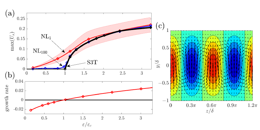
Figure 1: Analysis of roll/streak formation from an statistical state dynamics (SSD) bifurcation in a minimal channel Couette flow forced by background turbulence. Panel (a): streak amplitude, $U_{s}$, as a function of the stochastic excitation amplitude, $\varepsilon$, revealing the bifurcation as predicted by S3T (black) and the reflection of this prediction in an NL₁ simulation (red) and in an NL₁₀₀ simulation (blue). The NL₁ simulations exhibit fluctuations from the analytical predicted roll/streak structure with one standard deviation of the fluctuations indicated by shading. The critical value $\varepsilon_{c}$ is obtained from S3T stability analysis of the spanwise homogeneous state. The underlying S3T eigenmode is shown in panel (b) and its growth rate in (c). In panel (b) streak velocity, $U_{s}$, is indicated by contours and the velocity components $(V,W)$ by vectors. At $\varepsilon=\varepsilon_{c}$ the S3T spanwise uniform equilibrium bifurcates to a finite amplitude equilibrium with perturbation structure close to that of the most unstable eigenfunction shown in (b). The channel is minimal with $L_{x}=1.75\pi$ and $L_{z}=1.2\pi$ [50], the Reynolds number is $Re=400$, and the stochastic forcing excites only Fourier components with streamwise wave number $k_{x}=2\pi/L_{z}=1.143$. Numerical calculations employ $N_{y}=21$ grid points in the cross-stream direction and $32$ harmonics in the spanwise and streamwise directions (Adapted from [51]).

Streamwise roll vortices and associated streamwise streaks are prominent features in transitional boundary layers  [52]. The ubiquity of the roll/streak structure in these flows presents a problem because the laminar solution of these flows is linearly stable. However, because of the high non-normality of the Navier-Stokes (NS) dynamics linearized about a strongly sheared flow streamwise constant structures such the roll/streak have the greatest transient growth providing an explanation for its arising from perturbations to the flow [53, 54]. However, stochastic structural stability theory (S3T) reveals that the roll/streak structure is destabilized by systematic organization by the streak of the perturbation Reynolds stress associated with low levels of background turbulence [22]. Destabilization of the roll/streak can be traced to a universal positive feedback mechanism operating in turbulent flows: the coherent streak distorts the incoherent turbulence so as to induce ensemble mean perturbation Reynolds stresses that force streamwise mean roll circulations configured to reinforce the streak (cf. [22]). The modal streak perturbations of the fastest growing eigenfunctions induce the strongest such feedback. This instability does not have analytical expression in eigenanalysis of the NS dynamics but it can be solved for by performing an eigenanalysis on the S3T system.

Consider a laminar plane Couette flow subjected to stochastic excitation that is statistically streamwise and spanwise homogeneous and has zero spatial and temporal mean. S3T predicts that a bifurcation occurs at a critical amplitude of excitation, $\varepsilon_{c}$, in which an unstable mode with roll/streak structure emerges ($\varepsilon_{c}$ corresponds to an energy input rate that would sustain background turbulence energy of $0.14\%$ of the laminar flow). As the excitation parameter, $\varepsilon$ in (13b), is increased finite amplitude roll/streak structures equilibrate from this instability [22]. While these equilibria underlie the dynamics of roll/streak formation in the pre-transitional flow, they are imperfectly reflected in individual realizations (cf. Refs. [9, 51]). One can compare this behavior to that of the corresponding Navier-Stokes (NS) solutions by defining the $N$ ensemble nonlinear system (NL_N) in analogy with RNL_N as follows:

$$\partial_{t}{{\bf U}}={\mathbf{P}_{L}}\left(-{\bf U}\cdot\nabla{\bf U}+\frac{1}{Re}\Delta{\bf U}-\left<\left<\bf{u}\cdot\nabla\bf{u}\right>_{x}\right>_{N}\right)~{}~{},$$ (15a)

$$\partial_{t}{{\mathbf{u}_{n}}}=\bm{\mathsf{A}}({\bf U})\mathbf{u}_{n}+\sqrt{\varepsilon}~{}\mathbf{f}_{n}-{\mathbf{P}_{L}}\left(\mathbf{u}_{n}\cdot\nabla{\mathbf{u}_{n}}-\left<\mathbf{u}_{n}\cdot\nabla{\mathbf{u}_{n}}\right>_{x}\right),~{}~{}(n=1,\dots,N)~{}.$$ (15b)

Note that as $N\to\infty$ this system provides the second-order statistical state dynamics of the Navier-Stokes (NS) without approximation. Fig. 1 compares the analytical bifurcation structure predicted by S3T, the quasi-equilibria obtained using a single realization of the Navier-Stokes (NL₁) and the near perfect reflection of the S3T bifurcation in a $100$ member Navier-Stokes ensemble (NL₁₀₀) (cf. Refs. [22, 51]).

With continued increase in $\varepsilon$ a second bifurcation occurs in which the flow transitions to a chaotic time-dependent state. For the parameters used in our example this second bifurcation occurs at $\varepsilon_{t}/\varepsilon_{c}=5.5$. Once this time-dependent state is established the stochastic forcing can be removed and this state continues to be maintained as a self-sustaining turbulence. Remarkably, this self-sustaining turbulence naturally simplifies further by evolving to a minimal turbulent system in which the dynamics is supported by the interaction of the roll-streak structures with a perturbation field comprising a small number of streamwise harmonics (as few as 1). This minimal self-sustaining turbulent system, which proceeds naturally from the S3T dynamics, reveals an underlying self-sustaining process (SSP) which can be understood with clarity. The basic ingredient of this SSP is the robust tendency for streaks to organize the perturbation field so as to produce streamwise Reynolds stresses supporting the streak, as in the S3T instability mechanism shown Fig. 1c. Although the streak is strongly fluctuating in the self-sustaining state, the tendency of the streak to organize the perturbation field is retained. It is remarkable that the perturbations, in this highly time-dependent state, produce torques that maintain the streamwise roll not only on average but at nearly every instant. As a result, in this self-sustaining state, the streamwise roll is systematically maintained by the robust organization of perturbation Reynolds stress by the time-dependent streak while the streak is maintained by the streamwise roll through the lift-up mechanism [22, 23]. Through the resulting time-dependence of the roll-streak structure the constraint on instability imposed by the absence of inflectional instability in the mean flow is bypassed as the perturbation field is maintained by parametric growth [22, 55].

4 Self-sustaining turbulence in a restricted nonlinear model

The previous sections demonstrated that the stochastic structural stability theory (S3T) system (13) provides an attractive theoretical framework for studying turbulence through analysis of its underlying statistical mean state dynamics. However, it has the perturbation covariance as a variable and its dimension, which is O($N^{2}$) for a system of dimension O($N$), means that it is directly integrable only for low order systems. In this section we demonstrate that this computational limitation can be overcome by instead simulating the $N$ ensemble member RNL_N (14), using a finite number of realizations of the perturbation field (14b). In particular, we perform computations for a plane Couette flow at $Re=1000$, which show that a single realization ($N=1$) suffices to approximate the ensemble covariance allowing computationally efficient studies of the dynamical restriction underlying the S3T dynamics. We then demonstrate that the single ensemble member RNL₁ (which we interchangeably refer to as the RNL system) reproduces self-sustaining turbulent dynamics that reproduce the key features of turbulent plane Couette flow at low Reynolds numbers. We show that in correspondence with the S3T results, RNL turbulence is supported by a perturbation field comprising only a few streamwise varying modes (harmonics or $k_{x}\neq 0$ Fourier components in a Fourier representation) and that its streamwise wave number support can be reduced to a single streamwise varying mode interacting with the streamwise constant mean flow.

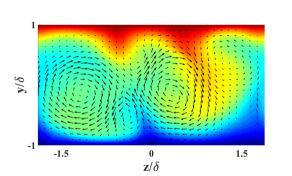
(a)  S3T

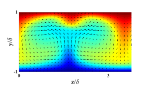
(b)  RNL

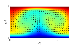
(c)  DNS

Figure 2: A $y$-$z$ plane cross-section of the flow (at $x$ = 0) at a single snapshot in time for (a) a S3T simulation, (b) a RNL simulation and (c) DNS data. All panels show contours of the streamwise component of the mean flow $U$ with the velocity vectors $V$, $W$ superimposed. The RNL and S3T dynamics are self-sustaining for the time shown.

We initiate turbulence in all of the RNL plane Couette flow simulations in this section by applying a stochastic excitation $\mathbf{f}$ in (14b) over the interval $t\in[0,500]$. We apply a similar procedure to initiate turbulence in the DNS, through $\mathbf{f}$ in (1), and S3T simulations, through its spatial covariance $\mathbf{Q}(1,2)$ in (13b). All results reported are for $t>1000$, unless otherwise stated. The DNS results are obtained from the Channelflow NS solver [56, 57], which is a pseudospectral code. The RNL simulations use a modified version of the same code. Complete details are provided in [19].

A comparison of the velocity field obtained from S3T and RNL₁ simulations that have reached self-sustaining states (i.e. for is $t>1000$) is shown in figures 2(a) and 2(b). These panels depict contour plots of an instantaneous snapshot of the streamwise component of the mean velocity with the vectors indicating velocity components ($V$, $W$) superimposed for the respective S3T and RNL flows at $Re=600$ in a minimal channel, see the caption in Figure 1 for the details. The same contour plot for a DNS is provided in figure 2(c) for comparison. These plots demonstrate the qualitative similarity in the structural features obtained from an S3T simulation, where the mean flow is driven by the full covariance, and the RNL simulation in which the covariance is approximated with a single realization of the perturbation field. Both flows also show good qualitative agreement with the DNS data.

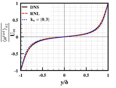
(a)

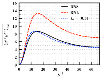
(b)

Figure 3: (a) Turbulent mean velocity profiles (based on streamwise, spanwise and time averages) in geometric units obtained from the DNS (red solid line) and RNL simulations with no band-limiting (black dashed line) and one where the streamwise wave number support is limited to $k_{x}=[0,3]$ (blue dotted line). All at $R=1000$. (b) Reynolds stresses $\overline{\langle u^{\prime+}u^{\prime+}}\rangle_{xz}$, where $u^{\prime}$ = $u^{tot}-\overline{u^{tot}}$ and $u^{+}$ = $u/u_{\tau}$. The figure in panel (a) is adapted from [19].

Having established the ability of the RNL system to provide a good qualitative approximation of the S3T turbulent field, we now proceed to discuss the features of RNL turbulence. For this discussion we move away from the minimal box at $Re=600$ that was used to facilitate comparison with the S3T equations and instead study plane Couette flow at $Re=1000$ in a box with respective streamwise and spanwise extents of $L_{x}=4\pi\delta$ and $L_{z}=4\pi\delta$. The turbulent mean velocity profile obtained from a DNS and a RNL simulation under these conditions is shown in Figure 3(a), which illustrates good agreement between the two turbulent mean velocity profiles. Figure 3(b) shows the corresponding time-averaged Reynolds stress component, $\overline{\langle u^{\prime+}u^{\prime+}}\rangle_{xz}$, where the streamwise fluctuations, $u^{\prime}$, are defined as $u^{\prime}$ = $u^{tot}-\overline{u^{tot}}$, $u^{+}$ = $u/u_{\tau}$ and $y^{+}$ = $(y+1)\hskip 0.85358ptu_{\tau}/\nu$ with friction velocity $u_{\tau}$ = $\sqrt{\tau_{w}/\rho}$, (where $\tau_{w}$ is the shear stress at the wall), $Re_{\tau}$ = $u_{\tau}\delta/\nu$ and $\nu$ = $1/Re$. The friction Reynolds numbers for the DNS data and the RNL simulation are respectively, ${Re_{\tau}}$ = $66.2$ and ${Re_{\tau}}$ = $64.9$. Although they are not shown here, previous studies have also shown close agreement between the Reynolds shear stress $\overline{u^{\prime}v^{\prime}}$ obtained from the RNL simulation and DNS [19], which is consistent with the fact that the turbulent flow supported by DNS and the RNL simulation exhibit nearly identical shear at the boundary, as seen in Figure 3(a). The close correspondence in the mean profiles in Figure 3(a), the $\overline{u^{\prime}v^{\prime}}$ Reynolds stresses reported in [19], as well as in the close correspondence values of $Re_{\tau}$ in the RNL simulations and DNS indicate that the overall energy dissipation rates per unit mass $\mathcal{E}=\tau_{w}{U}/{\delta}$, where ${U}/{\delta}$ is a constant based on the velocity of the walls $U$ and the half-height of the channel $\delta$, also show close correspondence.

Figure 3(b) shows that the peak magnitude of the streamwise component of the time-averaged Reynolds stresses, $\overline{\left<u^{\prime+}u^{\prime+}\right>_{xz}}$, is too high in the RNL simulation. Other second order statistics the premultiplied streamwise and spanwise spectra for this particular flow are presented in [19]. The discrepancies in both $\overline{\left<u^{\prime+}u^{\prime+}\right>_{xz}}$ and the streamwise premultiplied spectra reported are a direct result of the dynamical restriction, which results in a reduced number of streamwise wave numbers that support RNL turbulence, which we discuss next. In particular, we demonstrate that when $\mathbf{f}$ in equation (14b) is set to 0, the RNL model reduces to a minimal representation in which only a finite number of streamwise varying perturbations are maintained while energy in the other streamwise varying perturbations decays exponentially. This resulting limited streamwise wave number support cannot and is not expected to accurately reproduce the entire streamwise spectra but instead captures the spectral components associated with the turbulent structures that are responsible for the self-sustaining process, i.e. those corresponding to the spanwise streak and roll.

In order to frame our discussion of the streamwise wave number support of RNL turbulence we define a streamwise energy density associated with each perturbation wave number $k_{n},\,(n\neq 0)$ based on the perturbation energy of the associated streamwise wavelength $\lambda_{n}$ as

$$E_{\lambda_{n}}(t)=\int_{-1}^{1}\frac{1}{4}\langle||\mathbf{u}_{\lambda_{n}}(y,z,t)||^{2}\rangle_{z}\ dy.$$ (16)

Here $\mathbf{u}_{\lambda_{n}}$ is the perturbation, $\mathbf{u}=(u,v,w)$, associated with Fourier components with streamwise wavelength $\lambda_{n}$. We refer to the set of streamwise wave numbers for which $E_{\lambda_{n}}(t)$ does not tend to zero when $\mathbf{f}=0$ in equation (14b), as the natural support for the RNL system.

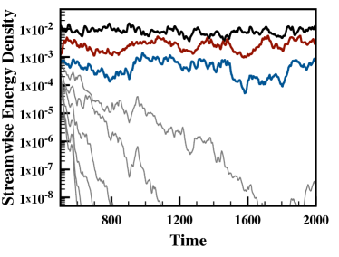
(a)

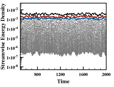
(b)

Figure 4: Streamwise energy densities for (a) a RNL simulation and (b) a DNS starting at $t=500$, when the stochastic excitation was terminated. The energy densities of the streamwise varying perturbations that are supported in the RNL simulation are shown in the following manner $\lambda_{1}$ = 4$\pi\delta$ (black), $\lambda_{2}$ = 2$\pi\delta$ (red), $\lambda_{3}$ = 4$\pi\delta/3$ (blue). The modes that decay when the RNL is in a self-sustaining state are shown in grey in both panels.

Figures 4(a) and 4(b) shows the time evolution of the streamwise energy densities $E_{\lambda_{n}}$ for a DNS and a RNL simulation, respectively. The simulations were both initiated with a stochastic excitation containing a full range of streamwise and spanwise Fourier components that was applied until $t=500$. Figure 4(a) illustrates that the streamwise energy density of most of the modes in the RNL simulation decay once the stochastic excitation is removed. The decay of these modes is a result of the dynamical restriction not an externally imposed modal truncation. As a result, the self-sustaining turbulent behavior illustrated in Figure 3 is supported by only 3 streamwise varying modes. In contrast, all of the perturbation components remain supported in the DNS. This behavior highlights an appealing reduction in model order in a RNL₁ simulation, which is consistent with the order reduction obtained when $N\to\infty$ [22].

We now demonstrate that RNL turbulence can be supported even when the perturbation dynamics (14b) are further restricted to a single streamwise Fourier component. This restriction to a particular wave number or set of wave numbers is accomplished by slowly damping the other streamwise varying modes as described in [24]. We refer to a RNL₁ system that is truncated to a particular set of streamwise Fourier components as a band-limited RNL model and those with no such restriction as baseline RNL systems.

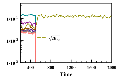
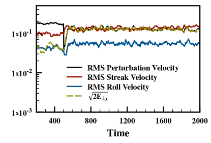
Figure 5: Sustaining turbulence with a single streamwise varying mode. (a) The RMS velocity of the streamwise energy density, $\sqrt{2E_{\lambda_{n}}}$, contained in each of the streamwise varying modes versus time before and after broad spectrum forcing is removed at $t=500$. The remaining mode $k_{x}=3$ ($\lambda_{3}=4\pi\delta/3$) is shown in gold. After the forcing is removed the remaining mode increases its energy to compensate for the loss of the other modes. (b) $\sqrt{2E_{\lambda_{n}}}$ for the undamped wavelength along with the RMS perturbation velocity, $U_{pert}$, the RMS streak velocity, $U_{streak}$, and the RMS roll velocity, $U_{roll}$, for the same data as in (a).

Thomas et al. [24] showed that band-limited RNL systems produce mean profiles and other structural features that are consistent with the baseline RNL system. Here we discuss only a subset of those results focusing on the particular case in which we keep only the $k_{x}=3$ mode corresponding to $\lambda=4\pi/3\delta$. Figure 5 shows the time evolution of the RMS velocity associated with the streamwise energy density, $\sqrt{2E_{\lambda_{3}}}$. The figure begins just prior to the removal at $t=500$ of the full spectrum stochastic forcing used to initialize the turbulence. At $t=500$ all but the perturbations associated with streamwise wave number $k_{x}=3$ are removed. It is interesting to note that once these streamwise wave numbers are removed the energy density of the remaining mode increases to maintain the turbulent state. This behavior can be further examined in the evolution of the RMS velocities of the streak, roll and perturbation energies over the same time period, which are respectively defined as $U_{streak}=\sqrt{2E_{s}}$, $U_{roll}=\sqrt{2E_{r}}$ and $U_{pert}=\sqrt{2E_{p}}$, where $E_{s}$, $E_{r}$ and $E_{p}$ are respectively defined in equations (4) - (6) shown in Figure 5. Here it is clear that after a small transient phase the roll and streak structures supported through the $k_{x}=3$ perturbation field increase to the levels maintained by the larger number of perturbation components present prior to the band-limiting.

Figure 3(b) also shows that the streamwise component of the normal Reynolds stress obtained in this band-limited system shows better agreement with the DNS than does the baseline RNL system. This behavior can be explained by looking at Figure 5, which shows that once the forcing is removed the total perturbation energy (as seen through $U_{pert}$) falls only slightly. This small drop is likely due to the removal of the forcing. This is consistent with observations that baseline and band-limited RNL simulations have approximately the same perturbation energy. The lower turbulent kinetic energy in Figure 3(b) for the band-limited system can be attributed to the increase in dissipation that results from forcing the flow to operate with only the shorter wavelength (higher wave number) structures.

5 RNL turbulence at moderate Reynolds numbers

The previous section demonstrates that the low order statistics obtained from RNL₁ simulations of low Reynolds number plane Couette flow show good agreement with DNS. We now discuss how the insight gained at low Reynolds numbers can be applied to simulations of half channel flows at moderate Reynolds numbers. The half-channel flow equations are given by equation (1) with a constant pressure gradient $\partial_{x}p_{\infty}$, a characteristic velocity $U_{m}$ equal to velocity at the top of the half-channel for the laminar flow, and the characteristic length $\delta$ equal to the full half-channel height. No-slip and stress-free boundary conditions are imposed at the respective bottom and top walls. As in the previous configurations periodic boundary conditions are imposed in the streamwise and spanwise directions. Further details regarding the half-channel simulations are provided in [25]. All results reported in this section are for $\varepsilon=0$.

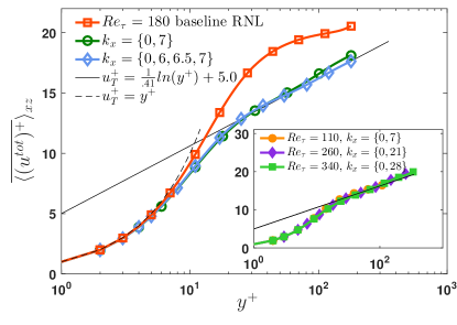
(a)

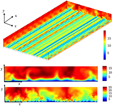
(b)

Figure 6: (a) Mean velocity profiles for baseline and band-limited RNL simulations at $Re_{\tau}=180$ in the forefront, and band-limited simulations at $Re_{\tau}=110,\,260$ and $340$ in the inset. (b) (Top) Snapshot of the streamwise velocity at a horizontal plane of $y^{+}=15$ for a band-limited RNL flow at Re${}_{\tau}=180$ with only $k_{x}=\{0,6,13,14\}$ . Cross-stream snapshots at Re${}_{\tau}=110$ (center) and Re${}_{\tau}=340$ (bottom) with respective streamwise wave numbers support sets of $k_{x}=\{0,7\}$ and $k_{x}=\{0,28\}$. This figure is adapted from [25], where the wave numbers reported there have been rescaled so that $k_{x}=1$ corresponds to $\lambda_{x}=4\pi\delta$ in order to be consistent with the previous section.

Previous studies of RNL simulations in Pouseuille flow (a full channel) with $\varepsilon=0$ have demonstrated that the accuracy of the mean velocity profile degrades as the Reynolds number is increased [23, 26]. This deviation from the DNS mean velocity profile is also seen in simulations of a half channel at $Re_{\tau}=180$, as shown in Figure 6(a). However, the previously observed ability to modify the flow properties through band-limiting the perturbation field can be exploited to improve the accuracy of the RNL predictions. Mean velocity profiles from a series of band-limited RNL simulations at Reynolds numbers ranging from $Re_{\tau}=180$ to $Re_{\tau}=340$ in which the improved accuracy over baseline RNL simulations is clear are shown in Figure 6(a). In particular, the mean profiles over this Reynolds number range exhibit a logarithmic region with standard values of $\kappa=0.41$ and $B=5.0$. It should also be noted that many of these band-limited RNL simulations have perturbation fields that are supported by a single streamwise varying wave number, although increasing the support to include a set of three adjacent $k_{x}\neq 0$ wave numbers results in slightly improved statistics at $Re_{\tau}=180$. Similar improvements are seen in the second-order statistics as reported in [25]. The specific wave number to be retained in the model in order to produce the results shown here were determined empirically by comparing the skin friction coefficient of the band-limited RNL profiles and those obtained from a well validated DNS [58]. That work demonstrated that the wave length producing the best fit over the range of Reynolds numbers shown scales with Reynolds number and asymptotes to a value of approximately $\lambda_{x}=150$ wall units. Preliminary work at higher Reynolds numbers has shown that this trend appears to continue to higher Reynolds numbers, although multiple wave numbers (of the same approximate wave length) may be needed. Developing the theory underlying this behavior is a direction of continuing work.

Figure 6(b) shows snapshots of the streamwise velocity fields for three of the band-limited RNL flows shown in Figure 6(a). The top image shows a horizontal ($x-z$) plane snapshot of the streamwise velocity, $u^{tot}$, at $y^{+}=15$ at $Re_{\tau}=180$ while the middle and bottom images depict cross plane ($y-z$) snapshots of the flow fields at $Re_{\tau}=110$ and $Re_{\tau}=340$, respectively. These images demonstrate realistic vortical structures in the cross-stream, while the band-limited nature of the streamwise-varying perturbations and the associated restriction to a particular set of streamwise wavelengths is clearly visible in the horizontal plane. The agreement of the transverse spatial structure of the fluctuations can be quantified through the comparisons of the spanwise spectra with DNS shown in Figure 7. Here we report results at two distances from the wall for the $Re_{\tau}=180$ data for the band-limited RNL simulation supported by a perturbation field limited to $k_{x}=14$ and a DNS at the same Reynolds number [58]. Although there are some differences in the magnitudes of the spectra, especially at low wave numbers, the qualitative agreement is very good considering the simplicity of the RNL model compared to the NS equations. The benefit of the RNL approach is that these results are obtained at a significantly reduced computational costs.

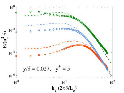
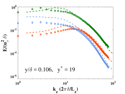
(a)                                   (b)

Figure 7: Spanwise energy spectra, $E_{uu}$ (green circles), $E_{vv}$ (red squares) and $E_{ww}$ (blue diamonds), obtained from the band-limited RNL model at Re${}_{\tau}=180$, at two wall-normal locations. The RNL system is constrained to a single perturbation wave number of $k_{x}=7$. Dashed lines are channel flow DNS data from Moser et al.[58] Symbols are RNL data. This figure is from [25].

6 Conclusion

Adopting the perspective of statistical state dynamics (SSD) provides not only new concepts and new methods for studying the dynamics underlying wall-turbulence but also new reduced order models for simulating wall-turbulence. The conceptual advance arising from SSD that we have reviewed here is the existence of analytical structures underlying turbulence dynamics that lack expression in the dynamics of realizations. The example we provided is that of the analytical unstable eigenmode and associated bifurcation structure associated with insatiability of the roll/streak structure in boundary layers subject to which has no analytical expression in the dynamics of realizations. The modeling advance that we reviewed is the naturally occurring reduction in order of RNL turbulence that allows construction of low dimensional models for simulating turbulence. These models are obtained through a dynamical restriction of the NS equations that forms a SSD or an approximation based on a finite number of realizations of the perturbation field all having a common mean flow, the restricted nonlinear RNL model. A RNL system with an infinite number of realizations, referred to as S3T, provides the conceptual advance, while the RNL approximation provides an efficient computational tool. The computational simplicity and the ability to band-limit the streamwise wave number support to improve the accuracy means that RNL simulations promise to provide a computationally tractable tool for probing the dynamics of high Reynolds number flows. The SSD perspective provides a set of tools that can provide new insights into wall-turbulence.

The author order is alphabetical. Sections 1-3 were primarily written by BFF and PJI with input by DFG. Sections 4 and 5 were written by DFG with input by BFF and PJI. Partial support from the National Science Foundation under AGS-1246929 (BFF) and a JHU Catalyst Award (DFG) is gratefully acknowledged. The authors would like to thank Charles Meneveau, Navid Constantinou and Vaughan Thomas for a number of helpful discussions and insightful comments on the manuscript.

References

- [1] Kim J, Moin P, Moser R. 1987 Turbulence statistics in fully developed channel flow at low Reynolds number, J. Fluid Mech. 177, 133–166.
- [2] del Álamo JC, Jiménez J, Zandonade P, Moser RD. 2004 Scaling of the energy spectra of turbulent channels, J. Fluid Mech. 500, 135–144.
- [3] Tsukahara T, Kawamura H, Shingai K. 2006 DNS of turbulent Couette flow with emphasis on the large-scale structure in the core region, J. Turbulence 7.
- [4] Wu X, Moin P. 2009 Direct numerical simulation of turbulence in a nominally zero-pressure-gradient flat-plate boundary layer, J. Fluid Mech. 630, 5–41.
- [5] Scott RK, Polvani LM. 2008 Equatorial superrotation in shallow atmospheres, Geophys. Res. Lett. 35, L24202.
- [6] Lee M, Moser RD. 2015 Direct numerical simulation of turbulent channel flow up to , J. Fluid Mech. 774, 395–415.
- [7] Hopf E. 1952 Statistical hydromechanics and functional calculus, J. Ration. Mech. Anal. 1, 87–123.
- [8] Frisch U. 1995 Turbulence: The Legacy of A. N. Kolmogorov. Cambridge University Press.
- [9] Farrell BF, Ioannou PJ. 2003 Structural stability of turbulent jets, J. Atmos. Sciences 60, 2101–2118.
- [10] Farrell BF, Ioannou PJ. 2007 Structure and spacing of jets in barotropic turbulence, J. Atmos. Sciences 64, 3652–3665.
- [11] Farrell BF, Ioannou PJ. 2009 A theory of baroclinic turbulence, J. Atmos. Sciences 66, 2444–2454.
- [12] Bakas NA, Ioannou PJ. 2011 Structural stability theory of two-dimensional fluid flow under stochastic forcing, J. Fluid Mech. 682, 332–361.
- [13] Bakas NA, Ioannou PJ. 2013 Emergence of large scale structure in barotropic -plane turbulence, Phys. Rev. Lett. 110, 224501.
- [14] Srinivasan K, Young WR. 2012 Zonostrophic instability, J. Atmos. Sciences 69, 1633–1656.
- [15] Gayme DF, McKeon BJ, Papachristodoulou A, Bamieh B, Doyle JC. 2010 A streamwise constant model of turbulence in plane Couette flow, J. Fluid Mech. 665, 99–119.
- [16] Farrell BF, Ioannou PJ. 1993 Stochastic forcing of the linearized Navier-Stokes equations, Phys. Fluids A 5, 2600–2609.
- [17] DelSole T, Farrell BF. 1996 The quasi-linear equilibration of a thermally mantained stochastically excited jet in a quasigeostrophic model, J. Atmos. Sciences 53, 1781–1797.
- [18] DelSole T. 2004 Stochastic models of quasigeostrophic turbulence, Surv. Geophys. 25, 107–149.
- [19] Thomas V, Lieu BK, Jovanović MR, Farrell BF, Ioannou P, Gayme DF. 2014 Self-sustaining turbulence in a restricted nonlinear model of plane Couette flow, Phys. Fluids 26, 105112.
- [20] Marston JB, Conover E, Schneider T. 2008 Statistics of an unstable barotropic jet from a cumulant expansion, J. Atmos. Sciences 65, 1955–1966.
- [21] Tobias SM, Dagon K, Marston JB. 2011 Astrophysical fluid dynamics via direct numerical simulation, Astrophys. J. 727, 127.
- [22] Farrell BF, Ioannou PJ. 2012 Dynamics of streamwise rolls and streaks in wall-bounded shear flow, J. Fluid Mech. 708, 149–196.
- [23] Constantinou NC, Lozano-Durán A, Nikolaidis MA, Farrell BF, Ioannou PJ, Jiménez J. 2014 Turbulence in the highly restricted dynamics of a closure at second order: Comparison with DNS, J. Phys.: Conf. Series 506, 012004.
- [24] Thomas V, Farrell B, Ioannou P, Gayme DF. 2015 A minimal model of self-sustaining turbulence, Phys. Fluids 27, 105104.
- [25] Bretheim JU, Meneveau C, Gayme DF. 2015 Standard logarithmic mean velocity distribution in a band-limited restricted nonlinear model of turbulent flow in a half-channel, Phys. Fluids 27, 011702.
- [26] Farrell BF, Ioannou PJ, Jiménez J, Constantinou NC, Lozano-Durán A, Nikolaidis MA. 2016 A statistical state dynamics-based study of the structure and mechanism of large-scale motions in plane Poiseuille flow, J. Fluid Mech. 809, 290–315.
- [27] Foias C, Manley O, Rosa R, Temam R. 2001 Navier-Stokes Equations and Turbulence. Cambridge University Press, Cambridge.
- [28] Monin AS, Yaglom AM. 1973 Statistical Fluid Mechanics: Mechanics of Turbulence, volume 1. The MIT Press.
- [29] Kim KJ, Adrian RJ. 1999 Very large scale motion in the outer layer, Phys. Fluids 11, 417–422.
- [30] Guala M, Hommema SE, Adrian RJ. 2006 Large-scale and very-large-scale motions in turbulent pipe flow, J. Fluid Mech. 554, 521–542.
- [31] Hutchins N, Marusic I. 2007 Evidence of very long meandering features in the logarithmic region of turbulent boundary layers, J. Fluid Mech. 579, 1–28.
- [32] Kline SJ, Reynolds WC, Schraub FA, Runstadler PW. 1967 The structure of turbulent boundary layers, J. Fluid Mech. 30, 741–773.
- [33] Komminaho J, Lundbladh A, Johansson A. 1996 Very large structures in plane turbulent Couette flow, J. Fluid Mech. 320, 259–285.
- [34] Blackwelder RF, Kaplan RE. 1976 On the wall structure of the turbulent boundary layer, J. Fluid Mech. 76, 89–112.
- [35] Bullock KJ, Cooper RE, Abernathy FH. 1978 Structural similarity in radial correlations and spectra of longitudinal velocity fluctuations in pipe flow, J. Fluid Mech. 88, 585–608.
- [36] Jovanović M, Bamieh B. 2005 Componentwise energy amplification in channel flows, J. Fluid Mech. 534, 145–183.
- [37] Cossu C, Pujals G, Depardon S. 2009 Optimal transient growth and very large scale structures in turbulent boundary layers, J. Fluid Mech. 619, 79–94.
- [38] Hwang Y, Cossu C. 2010 Amplification of coherent structures in the turbulent Couette flow: An input-output analysis at low Reynolds number, J. Fluid Mech. 643, 333–348.
- [39] Waleffe F. 1997 On a self-sustaining process in shear flows, Phys. Fluids A 9, 883–900.
- [40] Jiménez J, Pinelli A. 1999 The autonomous cycle of near-wall turbulence, J. Fluid Mech. 389, 335–359.
- [41] Hamilton K, Kim J, Waleffe F. 1995 Regeneration mechanisms of near-wall turbulence structures, J. Fluid Mech. 287, 317–348.
- [42] Hwang Y, Cossu C. 2010 Linear non-normal energy amplification of harmonic and stochastic forcing in the turbulent channel flow, J. Fluid Mech. 664, 51–73.
- [43] Hwang Y, Cossu C. 2010 Self-sustained process at large scales in turbulent channel flow, Phys. Rev. Lett. 105, 044505.
- [44] Reynolds WC, Kassinos SC. 1995 One-point modelling of rapidly deformed homogeneous turbulence, Proc. of the Royal Soc. of London. Series A: Mathematical and Physical Sciences 451, 87–104.
- [45] Bobba KM, Bamieh B, Doyle JC. 2002 Highly optimized transitions to turbulence. In Proc. of the IEEE Conf. on Decision and Control, pp. 4559–4562. Las Vegas, NV.
- [46] Bobba KM. 2004 Robust Flow Stability: Theory, Computations and Experiments in Near Wall Turbulence, Ph.D. thesis, California Institute of Technology, Pasadena, CA, USA.
- [47] Gayme DF. 2010 A Robust Control Approach to Understanding Nonlinear Mechanisms in Shear Flow Turbulence, Ph.D. thesis, Caltech, Pasadena, CA, USA.
- [48] Gayme DF, McKeon BJ, Bamieh B, Papachristodoulou A, Doyle JC. 2011 Amplification and nonlinear mechanisms in plane Couette flow, Phys. Fluids 23, 065108.
- [49] Bourguignon JL, McKeon BJ. 2011 A streamwise-constant model of turbulent pipe flow, Phys. Fluids 23, 095111.
- [50] Jiménez J, Moin P. 1991 The minimal flow unit in near-wall turbulence, J. Fluid Mech. 225, 213–240.
- [51] Farrell BF, Ioannou PJ, Nikolaidis MA. 2016 Instability of the roll/streak structure induced by free-stream turbulence in pre-transitional Couette flow, Phys. Rev. Fluids p. (Submitted arXiv:1607.05018).
- [52] Klebanoff PS, Tidstrom KD, Sargent LM. 1962 The three-dimensional nature of boundary-layer instability, J. Fluid Mech. 12, 1–34.
- [53] Butler KM, Farrell BF. 1992 Three-dimensional optimal perturbations in viscous shear flows, Phys. Fluids 4, 1637–1650.
- [54] Reddy SC, Henningson DS. 1993 Energy growth in viscous channel flows, J. Fluid Mech. 252, 209–238.
- [55] Farrell BF, Ioannou PJ. 2016 Structure and mechanism in a second-order statistical state dynamics model of self-sustaining turbulence in plane Couette flow, Phys. Rev. Fluids p. (Submitted arXiv:1607.05020).
- [56] Gibson JF. 2014 Channelflow: A spectral Navier-Stokes simulator in C++, Technical report, U. New Hampshire., Channelflow.org
- [57] Gibson JF, Halcrow J, Cvitanović P. 2008 Visualizing the geometry of state space in plane Couette flow, J. Fluid Mech. 611, 107–130.
- [58] Moser RD, Kim J, Mansour NN. 1999 Direct numerical simulation of turbulent channel flow up to , Phys. Fluids 11.