Preliminary Test and ‎‎Shrinkage Estimations of Scale Parameters for Two Exponential Distributions based on Record Values

Abstract

The exponential distribution is applied in a very wide variety of statistical procedures. Among the most prominent applications are those in the field of life testing and reliability theory. When there are two record samples available for estimating the scale parameter, a preliminary test is usually used to determine whether to pool the samples or use the individual sample. In this paper, the preliminary test estimator and shrinkage estimator are studied. The optimum level of significance for preliminary test estimation and the optimum values of shrinkage coefficient are obtained based on minimax regret criterion under the weighted square error loss function.

Keywords: Mean square error, Minimax regret criterion, Optimal significance level, Preliminary test estimation, Record values, Shrinkage estimator.

‎

1 Introduction

‎ Record values are of interest and important in many real life applications involving data relating to meteorology, sport, economics and life testing. Sometimes, the experimenter has some knowledge about the parameter of interest, either from past experience, or from experience with similar situations. This prior information may be incorporated in the estimation process using a preliminary test estimator (Ohtani and Toyoda, 1978; Toyoda and Wallace, 1975; Sawa and Hiromatsu, 1973; Chiou, 1990) and improved the estimation process. Preliminary test and shrinkage estimation in the one and two-parameter exponential distributions are considered by many authors including Pandey (1983) and Chiou and Han (1989).

Let $X_{1},X_{2},.....$ be a sequence of independent and identically distributed random variables having the same distribution. An observation $X_{j}$ will be called an upper record value if exceeds in value all of the preceding observations, i.e., if $X_{j}>X_{i}$, for every $i<j$. The sequence of record times is defined as follows: $T_{1}=1$ with probability 1 and, $T_{n}=\min\{j:X_{j}>X_{T_{n-1}}‎\}$ for $n\geq 2‎$. A sequence of upper record values is defined by $X_{U(n)}=X_{T_{n}}$‎, $n=1,2,\dots$‎. For details on record values and other interesting topics related to records see Ahsanullah (1995) and Arnold et al. (1998).

In this paper the estimation of the scale parameter in two exponential distributions based on record values is studied. When two record samples from exponential distributions are available, the question of whether to pool or not to pool these two record samples is often determined via a preliminary test. If the test is not statistically significant, the pooled estimator is used; otherwise, the likelihood estimator is used. The optimum level of statistical significance for the usual preliminary test estimator are obtained in Section 2 by using the minimax regret criterion. A shrinkage estimator is also considered. The optimum values of shrinkage coefficients for the shrinkage estimator are obtained in Section 3.‎ The proposed estimators are illustrated using an example, .and are compared using simulation in Section 4.

2 Preliminary test estimation

Let $X_{1},X_{2},\dots$ and $Y_{1},Y_{2},\dots$ be sequences of independent and identically distributed random variables from two exponential models with the following probability density function:

$$f_{X}(x)=\frac{1}{\theta_{1}}\exp(-\frac{x}{\theta_{1}})\ \ \ \ x>0,\ \ \ \ f_{Y}(y)=\frac{1}{\theta_{2}}\exp(-\frac{y}{\theta_{2}})\ \ \ \ y>0.$$

Also, suppose that we observe $n_{1}$ and $n_{2}$ upper record values from these two sequences as $\boldsymbol{X}=(X_{U(1)},\dots,X_{U(n_{1})})$ and $\boldsymbol{Y}=(Y_{U(1)},\dots,Y_{U(n_{2})})$. Therefore, the maximum likelihood estimations (MLE) of ‎$\theta_{1}$‎ and ‎$\theta_{2}$ are ‎‎‎‎

$$\hat{‎\theta‎}_{1}=‎\frac{1}{n_{1}}‎X_{U(n_{1})},\ \ \hat{‎\theta‎}_{2}‎=‎\frac{1}{n_{2}}‎Y_{U(n_{2})},$$

and $‎\frac{2‎n_{i}‎\hat{‎\theta‎}_{i}‎}{‎\theta_{i}‎}‎$ has the chi-square distribution with $2n_{i}$, $i=1,2$ degrees of freedom.

Assume that a prior information about the scale parameters is $\theta_{1}=‎\theta_{2}‎$. Then, the pooled estimator for $‎\theta_{1}‎$ (and $‎\theta_{2}‎$) is

$$‎\hat{‎\theta‎}_{p}‎=‎\frac{n_{1}‎\hat{‎\theta‎}_{1}+‎n_{2}‎\hat{‎\theta‎}_{2}}{n_{1}+n_{2}}‎.$$ (2.1)

To incorporate the prior information into the statistical procedure, a null hypothesis regarding the information is usually formulated and tested (see Bancroft, 1944; Bancroft and Han, 1977). Now consider testing $H_{0}:‎\theta_{1}=‎\theta_{2}$ against ‎‎$H_{1}:‎\theta_{1}‎\neq‎‎\theta_{2}$. If the null hypothesis is not rejected we use the pooled samples for estimating the scale parameter, but if the null hypothesis is rejected then we use the individual sample for estimating the parameter.

The likelihood ratio test reject $H_{0}$ when $‎‎\frac{‎\hat{‎\theta‎}_{1}‎}{‎\hat{‎\theta‎}_{2}‎}‎<c_{1}$ or $\frac{‎\hat{‎\theta‎}_{1}‎}{‎\hat{‎\theta‎}_{2}‎}>c_{2}$ where $c_{1}=F_{(2n_{1},2n_{2}),\alpha/2}$, $c_{2}=F_{(2n_{1},2n_{2}),1-\alpha/2}$. Therefore, a preliminary test estimator for $‎\theta‎_{1}$ may be obtained as follows

$$‎‎\hat{\theta}_{pt}=\left\{\begin{array}[]{lc}\hat{\theta}_{p}&\ \ c_{1}<\frac{\hat{\theta}‎_{1}}{\hat{\theta}‎_{2}}<c_{2}\\ \hat{\theta}_{1}&\ \ \ \text{otherwise}.\end{array}\right.$$ (2.2)

Similarly, a preliminary test estimator for $‎\theta‎_{2}$ can be obtained as

$$\hat{\theta}_{pt}^{*}=\left\{\begin{array}[]{lc}\hat{\theta}_{p}&\ \ c_{1}<\frac{\hat{\theta}‎_{1}}{\hat{\theta}‎_{2}}<c_{2}\\ \hat{\theta}_{2}&\ \ \ \text{otherwise}.\end{array}\right.$$ (2.3)

In the rest of this paper, we obtain the properties of preliminary test estimator $\hat{\theta}_{pt}$ and can use them for $\hat{\theta}_{pt}^{*}$.

The preliminary test estimator always depends on the significance level ($\alpha$) of the preliminary test. The methods to seek the optimal level of significance for the preliminary test have been investigated by Sawa and Hiromatsu (1973), Toyoda and Wallace (1975) and Ohtani and Toyoda (1978). Hirano (1977) applied AIC (Akaike, 1998) to determine the optimal level of significance for the preliminary test.

Lemma 2.1.

For the preliminary test estimator of $‎\theta‎_{1}$ in (2.2), we have

i)

$$Bias_{\theta_{1}}(\hat{\theta}_{pt})=E(\hat{\theta}_{pt})-\theta‎_{1} =‎ -\lambda\left(\theta_{1}[I_{d_{2}}(n_{1}+1,n_{2})-I_{d_{1}}(n_{1}+1,n_{2})]\right)$$

$$+\lambda\left(\theta_{2}[I_{d_{2}}(n_{1},n_{2}+1)-I_{d_{1}}(n_{1},n_{2}+1)]\right),$$

ii)

$$MSE(\hat{\theta}_{pt}) = \frac{n_{1}+1}{n_{1}}\theta_{1}^{2}+(\lambda^{2}-2\lambda)\theta_{1}^{2}\frac{(n_{1}+1)}{n_{1}}[I_{d_{2}}(n_{1}+2,n_{2})-I_{d_{1}}(n_{1}+2,n_{2})]$$

$$+\lambda^{2}\theta_{2}^{2}\frac{(n_{2}+1)}{n_{2}}[I_{d_{2}}(n_{1},n_{2}+2)-I_{d_{1}}(n_{1},n_{2}+2)]$$

$$+2(\lambda-\lambda^{2})\theta_{1}\theta_{2}[I_{d_{2}}(n_{1}+1,n_{2}+1)-I_{d_{1}}(n_{1}+1,n_{2}+1)]-2\theta_{1}^{2}$$

$$-2\lambda\theta_{1}\theta_{2}[I_{d_{2}}(n_{1},n_{2}+1)-I_{d_{1}}(n_{1},n_{2}+1)]$$

$$+2\lambda\theta_{1}^{2}[I_{d_{2}}(n_{1}+1,n_{2})-I_{d_{1}}(n_{1}+1,n_{2})]+\theta_{1}^{2}.$$

where $\lambda={n_{2}}/{(n_{1}+n_{2})}$, $I_{d}(a,b)=\int_{0}^{d}x^{a-1}(1-x)^{b-1}dx$ is incomplete beta function, $d_{1}=1-\frac{n_{2}}{c_{1}n_{1}\delta}$ and $d_{2}=1-\frac{n_{2}}{c_{2}n_{1}\delta}$, and $\delta=\frac{\theta_{2}}{\theta_{1}}$.

Proof.

Let $A=\left\{\boldsymbol{X},\boldsymbol{Y}|\ c_{1}<\frac{\hat{\theta}‎_{1}}{‎\hat{\theta}‎_{2}}<c_{2}\right\}$ be the acceptance region. So

$$\hat{\theta}_{pt}=\frac{n_{1}\hat{\theta}_{1}+n_{2}\hat{\theta}_{2}}{n_{1}+n_{2}}I_{A}+\hat{\theta}_{1}I_{A^{c}}=\hat{\theta}_{1}-\lambda\hat{\theta}_{1}I_{A}+\lambda\hat{\theta}_{2}I_{A},$$

where $A^{c}$ is the complement of $A$. Then

$$E(\hat{\theta}_{pt}) =‎ \theta‎_{1}-\lambda\left(\theta_{1}[I_{d_{2}}(n_{1}+1,n_{2})-I_{d_{1}}(n_{1}+1,n_{2})]\right)$$

$$+\lambda\left(\theta_{2}[I_{d_{2}}(n_{1},n_{2}+1)-I_{d_{1}}(n_{1},n_{2}+1)]\right),$$

and

$$E(\hat{\theta}_{pt}^{2}) = ‎\frac{n_{1}+1}{n_{1}}‎\theta_{1}^{2}‎‎+(\lambda^{2}-2\lambda)\big{(}\theta_{1}^{2}\frac{(n_{1}+1)}{n_{1}}[I_{d_{2}}(n_{1}+2,n_{2})-I_{d_{1}}(n_{1}+2,n_{2})]\big{)}$$

$$+\lambda^{2}\big{(}\theta_{2}^{2}\frac{(n_{2}+1)}{n_{2}}[I_{d_{2}}(n_{1},n_{2}+2)-I_{d_{1}}(n_{1},n_{2}+2)]\big{)}$$

$$+2(\lambda-\lambda^{2})\big{(}\theta_{1}\theta_{2}[I_{d_{2}}(n_{1}+1,n_{2}+1)-I_{d_{1}}(n_{1}+1,n_{2}+1)]\big{)}.$$

Since

$$MSE(\hat{\theta}_{pt})=E(\hat{\theta}_{pt}^{2})-2\theta_{1}E(\hat{\theta}_{pt})+\theta_{1}^{2},$$

the proof is completed. ∎

Remark 2.1.

Under the weighted square error loss function $L(d;\theta)‎=‎\frac{(d-\theta)^{2}‎}{\theta‎^{2}}$, the risk function is

$$R_{\alpha‎‎}(‎\delta‎) = Risk(‎\hat{\theta}‎_{pt},\theta_{1}‎)$$

$$= \delta^{2}\big{[}\lambda^{2}\frac{(n_{2}+1)}{n_{2}}[I_{d_{2}}(n_{1},n_{2}+2)-I_{d_{1}}(n_{1},n_{2}+2)]\big{]}$$

$$+\delta\big{[}2(\lambda-\lambda^{2})[I_{d_{2}}(n_{1}+1,n_{2}+1)-I_{d_{1}}(n_{1}+1,n_{2}+1)]$$

$$-2\lambda[I_{d_{2}}(n_{1},n_{2}+1)-I_{d_{1}}(n_{1},n_{2}+1)]\big{]}$$

$$+\big{[}\frac{1}{n_{1}}+(\lambda^{2}-2\lambda)\frac{(n_{1}+1)}{n_{1}}[I_{d_{2}}(n_{1}+2,n_{2})-I_{d_{1}}(n_{1}+2,n_{2})]$$

$$+2\lambda[I_{d_{2}}(n_{1}+1,n_{2})-I_{d_{1}}(n_{1}+1,n_{2})]\big{]},$$

where $\delta=\frac{\theta_{2}}{\theta_{1}}$

Notice that the risk function depends on $‎\alpha$‎ through $c_{1}$ and $c_{2}$. If $‎\delta‎\rightarrow 0$ or $\infty$‎‎‎ then $R_{\alpha‎‎}(‎\delta‎)$ converges to $R_{1}(‎\delta‎)$ which is the risk for ‎$\hat{‎\theta‎}_{1}$. The general shapes of $R_{\alpha‎‎}(‎\delta‎)$ for fixed values of $n_{1}$, $n_{2}$ and some $‎\alpha‎$ are shown in Figure 1. Consider $\delta_{1}$ ‎and $\delta_{2}$ are intersections of $R_{0‎‎}(‎\delta‎)=({n_{1}+n_{2}\delta^{2}+n_{2}^{2}\delta^{2}+n_{2}^{2}-2n_{2}^{2}\delta})/{(n_{1}+n_{2})^{2}}‎$ and $R_{1‎‎}(‎\delta‎)=‎{1}/{n_{1}}‎$. Therefore, an optimal value of $\alpha$‎ is $\alpha=1$ if $\delta\leq\delta_{1}$‎‎‎ or $\delta\geq\delta_{2}$; it is $\alpha=0$, ‎otherwise. Since ‎$‎\delta‎$ is unknown, we try to find an optimum values $\alpha=\alpha^{*}$ which gives a reasonable risk for all values of $\delta$‎. ‎‎‎ The regret function is defined as ‎

$${Reg}(\delta,\alpha)=R_{\alpha‎‎}(‎\delta‎)-\inf_{\alpha}‎R_{\alpha‎‎}(‎\delta‎),$$

‎‎‎ where $\mathop{\inf}_{\alpha}R_{\alpha‎‎}(‎\delta‎)=R_{0‎‎}(‎\delta‎)$ for $\delta_{1}<\delta<\delta_{2}‎$, and $\mathop{\inf}_{\alpha}R_{\alpha‎‎}(‎\delta‎)=R_{1‎‎}(‎\delta‎)$, otherwise.

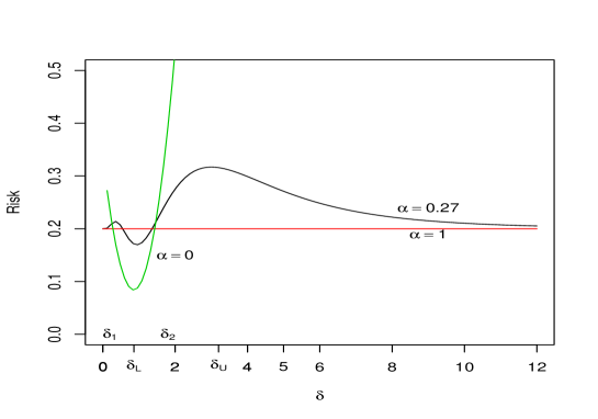
Figure 1: The risk function for some $\alpha$‎ with $n_{1}=5$ and $n_{2}=6$.

‎

Minimizing the maximum risk sometimes leads to unreasonable or trivial results, especially in prediction problems (see Hodges and Lehmann, 1950). In such a situation, we are often able to arrive at reasonable results by minimizing the maximum regret instead of the maximum risk. The minimax regret criterion determines $‎\alpha‎^{*}‎$ such that

$$\mathop{\sup}_{\delta}\{Reg(\delta,\alpha^{*}‎)\}‎‎\leq‎\mathop{\sup}_{\delta}\{Reg(\delta,\alpha)\},$$

for every significance level $\alpha\neq‎\alpha^{*}$. For $‎\delta‎\leq‎\delta_{2}$, $Reg(\delta,\alpha)$‎‎‎ takes a maximum value at $‎\delta_{L}$ based on Figure 1. Also, for $\delta>‎\delta_{2}$, $Reg(\delta,\alpha)$‎‎‎‎‎‎ ‎‎takes a maximum value at $‎\delta_{U}$.‎ Thus the minimax regret criterion determines $‎\alpha‎^{*}‎$‎ such that $Reg(\delta_{L},\alpha‎^{*}‎)=Reg(\delta_{U},\alpha‎^{*}‎)$. We found numerically the optimum significance level $‎\alpha‎^{*}‎$ for some $n_{1}$ and $n_{2}$. The results are given in Table 1.

Table 1: Optimal value $\alpha^{*}$ for some $n_{1}$ and $n_{2}$.

‎ $n_{1}$ $n_{{\rm 2}}$ 2 3 4 5 7 10 2 0.38 0.30 0.27 0.24 0.22 0.20 3 0.42 0.34 0.29 0.27 0.24 0.21 4 0.44 0.36 0.31 0.28 0.25 0.22 5 0.46 0.38 0.33 0.30 0.26 0.23 7 0.49 0.40 0.35 0.32 0.28 0.25 10 0.51 0.42 0.37 0.33 0.29 0.26

3 Shrinkage estimator

The shrinkage estimators have been discussed by a number of others, for details see Lehmann and Casella (1998), Prakash and Singh (2006, 2008, 2009). The preliminary test estimator given in Section 2 uses pooled estimator $\hat{\theta}_{p}‎$ when preliminary test accepts the null hypothesis. Instead of using $‎\hat{‎\theta‎}_{p}‎$, we can use a linear combination of $\hat{\theta}_{p}‎$ and $\hat{\theta}_{1}‎$ when the preliminary test accepts $H_{0}$, this gives a preliminary test shrinkage estimator which is smoother than the usual preliminary test estimator. The shrinkage estimator performs better than the usual estimator when the our guess is approximately true. Shrinkage estimators are usually defined as estimators obtained through modification of the usual (maximum likelihood, minimum variance unbiased, least squares, etc.) estimator in order to optimize some desirable criterion function.

Among various kinds of shrinkage estimators proposed so far, Jani (1991) and Kourouklis (1994) have suggested shrinkage estimators for the scale parameter in one and two-parameter exponential distributions. In this section, we study the preliminary test shrinkage estimator $\hat{\theta}_{S}$ following the same estimation procedure by Inada (1984):

$$‎‎\hat{\theta}_{S}=\left\{\begin{array}[]{lc}K\hat{\theta}_{p}+(1-K)\hat{\theta}_{1}&c_{1}<\frac{\hat{\theta}_{1}}{\hat{\theta}_{1}}<c_{2}\\ \hat{\theta}_{1}&\text{otherwise}.\end{array}\right.$$ (3.3)

If $K=1$, $‎‎\hat{‎\theta‎‎}_{S}$ reduce to $\hat{\theta}_{pt}$. The shrinkage coefficient $K$ is not defined explicitly as a function of the test statistic. The weighting function approach is intuitively appearing, but the mean square error of the resulting estimator usually cannot be derive unless the weighting function is in some simple form. Note that $‎\hat{‎‎\theta‎‎}‎_{pt}$ approaches $‎\theta_{0}$ as $‎‎\alpha‎\rightarrow 0$ ‎and it approaches $‎‎\hat{‎\theta‎}‎‎‎_{Ml}$ as $‎‎\alpha‎\rightarrow 1$, however $‎\hat{‎‎\theta‎‎}‎_{S}$ approaches $‎\hat{‎\theta‎}‎_{pt}$ as $‎‎K\rightarrow 1$ and it approaches $‎‎\hat{‎\theta‎}‎‎‎_{Ml}$ as $‎‎K‎\rightarrow 0$.‎ Unfortunately, different value of significance level $(‎\alpha)$ or‎ different value of shrinkage coefficient ($K$) induces a different estimator. the choice of these values depends on the decision criterion.

‎

Lemma 3.1.

For the shrinkage estimator of $‎\theta‎_{1}$ in (3.3)‎, we have

i)

$$Bias_{\theta_{1}}(\hat{\theta}_{S})=E(\hat{\theta}_{S})-\theta‎_{1} =‎ -K\lambda\big{(}\theta_{1}[I_{d_{2}}(n_{1}+1,n_{2})-I_{d_{1}}(n_{1}+1,n_{2})]\big{)}$$

$$+K\lambda\big{(}\theta_{2}[I_{d_{2}}(n_{1},n_{2}+1)-I_{d_{1}}(n_{1},n_{2}+1)]\big{)},,$$

ii)

$$MSE(\hat{\theta}_{S}) = \frac{n_{1}+1}{n_{1}}\theta_{1}^{2}+(K^{2}\lambda^{2}-2K\lambda)\theta_{1}^{2}\frac{(n_{1}+1)}{n_{1}}[I_{d_{2}}(n_{1}+2,n_{2})-I_{d_{1}}(n_{1}+2,n_{2})]$$

$$+K^{2}\lambda^{2}\theta_{2}^{2}\frac{(n_{2}+1)}{n_{2}}[I_{d_{2}}(n_{1},n_{2}+2)-I_{d_{1}}(n_{1},n_{2}+2)]$$

$$+2(K\lambda-K^{2}\lambda^{2})\theta_{1}\theta_{2}[I_{d_{2}}(n_{1}+1,n_{2}+1)-I_{d_{1}}(n_{1}+1,n_{2}+1)]-2\theta_{1}^{2}$$

$$-2K\lambda\theta_{1}\theta_{2}[I_{d_{2}}(n_{1},n_{2}+1)-I_{d_{1}}(n_{1},n_{2}+1)]$$

$$+2K\lambda\theta_{1}^{2}[I_{d_{2}}(n_{1}+1,n_{2})-I_{d_{1}}(n_{1}+1,n_{2})]+\theta_{1}^{2}.$$

Proof.

The straightforward evaluation leads to

$$E(\hat{\theta}_{S}) = ‎\theta‎_{1}-K\lambda\big{(}\theta_{1}[I_{d_{2}}(n_{1}+1,n_{2})-I_{d_{1}}(n_{1}+1,n_{2})]\big{)}$$

$$+K\lambda\big{(}\theta_{2}[I_{d_{2}}(n_{1},n_{2}+1)-I_{d_{1}}(n_{1},n_{2}+1)]\big{)},$$

and

$$E(\hat{\theta}_{S}^{2}) = ‎\frac{n_{1}+1}{n_{1}}‎\theta_{1}^{2}‎‎+(K^{2}\lambda^{2}-2K\lambda)\big{(}\theta_{1}^{2}\frac{(n_{1}+1)}{n_{1}}[I_{d_{2}}(n_{1}+2,n_{2})-I_{d_{1}}(n_{1}+2,n_{2})]\big{)}$$

$$+K^{2}\lambda^{2}\big{(}\theta_{2}^{2}\frac{(n_{2}+1)}{n_{2}}[I_{d_{2}}(n_{1},n_{2}+2)-I_{d_{1}}(n_{1},n_{2}+2)]\big{)}$$

$$+2(K\lambda-K^{2}\lambda^{2})\big{(}\theta_{1}\theta_{2}[I_{d_{2}}(n_{1}+1,n_{2}+1)-I_{d_{1}}(n_{1}+1,n_{2}+1)]\big{)}.$$

Since

$$MSE(\hat{\theta}_{S})=E(\hat{\theta}_{S}^{2})-2\theta_{1}E(\hat{\theta}_{S})+\theta_{1}^{2},$$

the proof is completed. ∎

Remark 3.1.

Under the weighted square error loss function $L(d;‎\theta)‎=‎\frac{(d-‎\theta)^{2}‎}{‎\theta‎^{2}}$, we have

$$R_{\alpha}(‎\delta,K) = ‎‎Risk(‎\hat{‎\theta‎}‎_{S},\theta_{1})$$

$$= \delta^{2}\big{[}K^{2}\lambda^{2}\frac{(n_{2}+1)}{n_{2}}[I_{d_{2}}(n_{1},n_{2}+2)-I_{d_{1}}(n_{1},n_{2}+2)]\big{]}$$

$$+\delta\big{[}2(K\lambda-K^{2}\lambda^{2})[I_{d_{2}}(n_{1}+1,n_{2}+1)-I_{d_{1}}(n_{1}+1,n_{2}+1)]$$

$$-2K\lambda[I_{d_{2}}(n_{1},n_{2}+1)-I_{d_{1}}(n_{1},n_{2}+1)]\big{]}$$

$$+\big{[}\frac{1}{n_{1}}+(K^{2}\lambda^{2}-2K\lambda)\frac{(n_{1}+1)}{n_{1}}[I_{d_{2}}(n_{1}+2,n_{2})-I_{d_{1}}(n_{1}+2,n_{2})]$$

$$+2K\lambda[I_{d_{2}}(n_{1}+1,n_{2})-I_{d_{1}}(n_{1}+1,n_{2})]\big{]}.$$

The regret function is defined as

$$Reg(‎\delta,K,‎\alpha)=R_{\alpha}(‎\delta,K)-\inf_{K}R_{\alpha}(‎\delta,K).$$

Since $R_{\alpha}(‎\delta,K)$ has quadratic form w.r.t $K$, so it has minimum in the interval [0,1]. Let $R_{\alpha}(‎\delta,K)=K^{2}h_{2}(‎\delta‎)‎‎+Kh_{1}(‎\delta‎)+h_{0}(‎\delta‎)$ then ‎$\frac{‎\partial R‎}{‎‎\partial K‎‎}=0‎$ imply that $K_{0}=‎\frac{-h_{1}(‎\delta‎)}{2h_{2}(‎\delta‎)}‎$‎‎ is an extremum point. Therefore

$$\inf_{K}R_{\alpha}(‎\delta,K)=\left\{\begin{array}[]{lc}\min\{R_{\alpha}(‎\delta,0),R_{\alpha}(‎\delta,1),R_{\alpha}(‎\delta,K_{0})\}‎‎‎&\text{if}\ \ K_{0}‎‎\in(0,1)‎‎\\ \min\{R_{\alpha}(‎\delta,0),R_{\alpha}(‎\delta,1)\}‎‎‎&\text{otherwise}.\end{array}\right.$$

‎ After rather extensive numerical investigation the values $K$ which attain the $\inf_{K}\sup_{‎\delta‎}Reg(‎\delta,$ $K,‎\alpha‎‎)$ are obtained. We plot the risk function for $n_{1}=5$, $n_{2}=6$, $‎\alpha=0.16‎$, for $K=0,1,0.21$ in Figure 2. Let $‎\delta_{1}$ and $‎\delta_{2}$ be intersections of $R_{\alpha}(‎\delta,0)$ and $R_{\alpha}(‎\delta,1)$. For $‎\delta‎\leq‎\delta_{2}$‎‎‎, $Reg(‎\delta,K,‎\alpha‎)$‎ takes a maximum value at $‎\delta_{L}$‎. For $‎\delta‎>‎\delta_{2}$‎‎‎, $Reg(‎\delta,K,‎\alpha‎)$‎ takes a maximum value at $‎\delta_{U}$. The reasonable estimator is obtained when these two maximum values are equal. Thus the minimax regret criterion determines $K^{*}$ such that:

$$Reg(‎\delta_{L},K^{*}‎)=Reg(‎\delta_{U},K^{*}‎).$$

To find the optimal value of $K$, two cases are considered for $‎\alpha$‎:

Case I: Let $‎\alpha=0.16‎$, that is the AIC optimal level of significance (see Inada, 1984), which is independent of $n$. Table 2 presents the values of $K^{*}$ for some $n_{1}$ and $n_{2}$.‎

Case II: ‎Let $‎\alpha=‎\alpha^{*}$ ‎equal the significance level of pre-test. Table 3 presents the values of $K^{*}$ in this case for some $n_{1}$ and $n_{2}$.

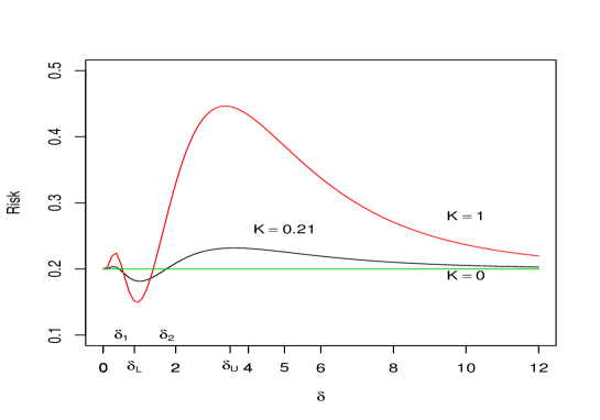
Figure 2: The risk function for some $K‎$ with $n_{1}=5$ and $n_{2}=6$.

‎

Table 2: Optimal value $K$ for some $n_{1}$ and $n_{2}$ with $‎\alpha=0.16‎$.‎‎

‎ $n_{1}$ $n_{2}$ 2 3 4 5 7 10 2 0.17 0.23 0.29 0.32 0.38 0.42 3 0.14 0.19 0.24 0.27 0.32 0.36 4 0.12 0.17 0.21 0.24 0.29 0.33 5 0.11 0.16 0.20 0.22 0.27 0.31 7 0.10 0.14 0.18 0.20 0.24 0.28 10 0.10 0.13 0.17 0.19 0.23 0.26

Table 3: Optimal value $K$ for some $n_{1}$ and $n_{2}$ with optimal $‎\alpha=‎\alpha^{*}‎‎$‎‎‎‎.

	$n_{1}=2$		$n_{1}=3$		$n_{1}=4$		$n_{1}=5$		$n_{1}=7$		$n_{1}=10$
$n_{2}$	${\alpha}^{*}$	$K^{*}$	${\alpha}^{*}$	$K^{*}$	${\alpha}^{*}$	$K^{*}$	${\alpha}^{*}$	$K^{*}$	${\alpha}^{*}$	$K^{*}$	${\alpha}^{*}$	$K^{*}$
2	0.38	0.21	0.30	0.29	0.27	0.34	0.24	0.37	0.22	0.42	0.20	0.45
3	0.42	0.15	0.34	0.23	0.29	0.28	0.27	0.31	0.24	0.35	0.21	0.39
4	0.44	0.12	0.36	0.19	0.31	0.24	0.28	0.27	0.25	0.32	0.22	0.35
5	0.46	0.11	0.38	0.17	0.33	0.22	0.30	0.25	0.26	0.29	0.23	0.33
7	0.49	0.10	0.40	0.15	0.35	0.19	0.32	0.22	0.28	0.26	0.25	0.30
10	0.51	0.09	0.42	0.14	0.37	0.17	0.33	0.20	0.29	0.24	0.26	0.28

Remark 3.2.

For the general case, if we observe upper record values $X_{U(1)},\dots,X_{U(n_{1})}$ and $Y_{U(1)},\dots,Y_{U(n_{2})}$ from location-scale exponential distribution with the following probability density function

$$f_{X}(x)=\frac{1}{\theta_{1}}\exp(-\frac{x-\eta_{1}}{\theta_{1}})\ \ \ \ x>\eta_{1},\ \ \ \ f_{Y}(y)=\frac{1}{\theta_{2}}\exp(-\frac{y-\eta_{2}}{\theta_{2}})\ \ \ \ y>\eta_{2},$$

the MLE’s of ‎$\theta_{1}$‎ and $\theta_{2}$ are ‎

$$\hat{‎\theta‎}_{1}=‎\frac{1}{n_{1}}(‎X_{U(n_{1})}-X_{U(1)}),\ \ \hat{‎\theta‎}_{2}‎=‎\frac{1}{n_{2}}(‎Y_{U(n_{2})}-‎Y_{U(1)}),$$

and ${2‎n_{i}‎\hat{‎\theta‎}_{i}‎}/{‎\theta_{i}‎}‎$ has the chi-square distribution with $2n_{i}-2$, $i=1,2$ degrees of freedom. In this case, we have the same result as the special case in absence of location parameter with a new statistic and degree of freedom.

4 Numerical study

In this section, we first illustrate the proposed estimators using an example. Then, these estimators are compared using simulation.

4.1 An example

The following the simulated record values are given by Baklizi (2013). The first record values which are generated from location-scale exponential distribution with $\theta_{1}=1$ and $\eta_{1}=3$ are 3.105, 6.158, 6.296, 6.824, 7.282, 10.200, 10.240, and 11.669, and first record values which are generated from location-scale exponential distribution with $\theta_{2}=1$ and $\eta_{2}=1$ are 1.177, 2.430, 4.090, 4.349, 4.624, 5.655, 6.021, and 6.987.

The MLE’s of $\theta_{1}$ and $\theta_{2}$ are $\hat{\theta}_{1}=1.0705$ and $\hat{\theta}_{2}=0.7262$. Since the hypothesis $H_{0}:\theta_{1}=\theta_{2}$ is not rejected the preliminary test and optimal shrinkage estimations are $\hat{\theta}_{pt}=0.8984$, and $\hat{\theta}_{S}=1.0292$, respectively. It can be seen that the optimal shrinkage estimation is very close to the true value $\theta_{1}=1$.

4.2 Simulation

We performed a simulation to compare the ML, preliminary test, and shrinkage estimators with 10000 repetition. First, a random sample with size $n_{1}$ is generated from an exponential distribution with scale parameter $\theta_{1}=1$. Then, a random sample with size $n_{2}$ is generated from an exponential distribution with scale parameter $\theta_{2}$. We consider some values between 0.1 and 3.0 for $\theta_{2}$. The estimators are calculated and their biases are obtained. Also, the efficiency of preliminary test, and shrinkage estimators with respect to MLE are computed (Here, the efficiency is ratio of MSEs). The results for $\alpha=0.16$ are given in Tables 4, and for the optimal $\alpha$ and $K$ (proposed in Table 3) are given in Table 5.

It can be concluded that
i. When $\theta_{1}$ and $\theta_{2}$ are very close, the preliminary test estimator is better than the shrinkage estimator. Also, the shrinkage estimator is better than the MLE. Therefore, the two proposed estimators are better that MLE when a prior information about the scale parameters is $\theta_{1}=\theta_{2}$.
ii. When $\theta_{1}$ and $\theta_{2}$ are not close, the MLE are better than the shrinkage estimator. Also, the shrinkage estimator is better than the preliminary test estimator.

Table 4: The simulation results with $\alpha=0.16$.

		Bias			Efficiency				Bias			Efficiency
$n_{1},n_{2}$	$\theta_{2}$	$\hat{\theta}_{1}$	$\hat{\theta}_{pt}$	$\hat{\theta}_{s}$	$\hat{\theta}_{pt}$	$\hat{\theta}_{s}$	$n_{1},n_{2}$	$\theta_{2}$	$\hat{\theta}_{1}$	$\hat{\theta}_{pt}$	$\hat{\theta}_{s}$	$\hat{\theta}_{pt}$	$\hat{\theta}_{s}$
2,2	0.1	-0.003	-0.003	-0.003	1.000	1.000	7,2	0.1	0.002	0.000	0.000	0.999	1.000
	0.3	-0.003	-0.022	-0.008	0.902	0.978		0.3	0.002	-0.018	-0.005	0.905	0.978
	0.5	-0.003	-0.056	-0.017	0.914	0.995		0.5	0.002	-0.054	-0.014	0.913	0.994
	0.8	-0.003	-0.042	-0.013	1.200	1.080		0.8	0.002	-0.036	-0.009	1.201	1.079
	1.0	-0.003	-0.006	-0.004	1.240	1.095		1.0	0.002	0.000	0.000	1.226	1.091
	1.2	-0.003	0.028	0.007	1.099	1.069		1.2	0.002	0.032	0.010	1.104	1.070
	1.5	-0.003	0.064	0.014	0.849	1.005		1.5	0.002	0.067	0.017	0.878	1.016
	2.0	-0.003	0.081	0.019	0.661	0.930		2.0	0.002	0.080	0.021	0.682	0.938
	2.5	-0.003	0.068	0.016	0.635	0.911		2.5	0.002	0.071	0.018	0.643	0.913
	3.0	-0.003	0.050	0.011	0.667	0.917		3.0	0.002	0.054	0.014	0.662	0.915
2,5	0.1	-0.001	0.002	0.002	1.000	1.000	7,5	0.1	0.001	0.003	0.003	0.999	1.000
	0.3	-0.001	-0.016	-0.002	0.903	0.977		0.3	0.001	-0.017	-0.002	0.901	0.977
	0.5	-0.001	-0.050	-0.011	0.925	0.997		0.5	0.001	-0.051	-0.011	0.922	0.997
	0.8	-0.001	-0.036	-0.008	1.201	1.078		0.8	0.001	-0.036	-0.007	1.207	1.080
	1.0	-0.001	0.000	0.002	1.244	1.094		1.0	0.001	0.001	0.002	1.230	1.091
	1.2	-0.001	0.032	0.010	1.112	1.075		1.2	0.001	0.035	0.012	1.093	1.066
	1.5	-0.001	0.069	0.020	0.857	1.007		1.5	0.001	0.068	0.020	0.873	1.013
	2.0	-0.001	0.084	0.024	0.684	0.938		2.0	0.001	0.087	0.025	0.671	0.934
	2.5	-0.001	0.076	0.021	0.636	0.910		2.5	0.001	0.073	0.021	0.646	0.915
	3.0	-0.001	0.055	0.016	0.673	0.919		3.0	0.001	0.055	0.017	0.664	0.915
2,10	0.1	-0.001	-0.001	-0.001	0.999	1.000	7,7	0.1	-0.005	0.001	0.001	1.000	1.000
	0.3	-0.001	-0.019	-0.005	0.903	0.978		0.3	-0.005	-0.018	-0.004	0.908	0.979
	0.5	-0.001	-0.055	-0.015	0.922	0.997		0.5	-0.005	-0.052	-0.013	0.914	0.994
	0.8	-0.001	-0.038	-0.010	1.191	1.077		0.8	-0.005	-0.038	-0.009	1.198	1.079
	1.0	-0.001	-0.003	-0.001	1.216	1.088		1.0	-0.005	-0.002	0.000	1.219	1.089
	1.2	-0.001	0.031	0.007	1.075	1.063		1.2	-0.005	0.030	0.006	1.094	1.068
	1.5	-0.001	0.064	0.016	0.880	1.014		1.5	-0.005	0.067	0.018	0.861	1.008
	2.0	-0.001	0.080	0.020	0.690	0.940		2.0	-0.005	0.081	0.022	0.683	0.938
	2.5	-0.001	0.072	0.018	0.638	0.912		2.5	-0.005	0.071	0.019	0.645	0.914
	3.0	-0.001	0.055	0.014	0.654	0.912		3.0	-0.005	0.056	0.015	0.656	0.913
10,2	0.1	-0.004	-0.002	-0.002	1.000	1.000	10,7	0.1	0.002	0.004	0.004	0.999	1.000
	0.3	-0.004	-0.020	-0.007	0.903	0.978		0.3	0.002	-0.015	-0.001	0.903	0.978
	0.5	-0.004	-0.054	-0.015	0.916	0.995		0.5	0.002	-0.049	-0.010	0.920	0.996
	0.8	-0.004	-0.036	-0.011	1.206	1.082		0.8	0.002	-0.035	-0.006	1.207	1.081
	1.0	-0.004	-0.004	-0.003	1.221	1.090		1.0	0.002	0.000	0.003	1.246	1.094
	1.2	-0.004	0.031	0.008	1.100	1.071		1.2	0.002	0.034	0.010	1.092	1.067
	1.5	-0.004	0.064	0.015	0.861	1.011		1.5	0.002	0.069	0.021	0.862	1.009
	2.0	-0.004	0.080	0.020	0.674	0.935		2.0	0.002	0.087	0.025	0.680	0.938
	2.5	-0.004	0.069	0.017	0.632	0.909		2.5	0.002	0.077	0.023	0.629	0.907
	3.0	-0.004	0.053	0.013	0.653	0.911		3.0	0.002	0.060	0.018	0.664	0.916

Table 5: The simulation results with optimal $\alpha$ and $K$.

		Bias			Efficiency				Bias			Efficiency
$n_{1},n_{2}$	$\theta_{2}$	$\hat{\theta}_{1}$	$\hat{\theta}_{pt}$	$\hat{\theta}_{s}$	$\hat{\theta}_{pt}$	$\hat{\theta}_{s}$	$n_{1},n_{2}$	$\theta_{2}$	$\hat{\theta}_{1}$	$\hat{\theta}_{pt}$	$\hat{\theta}_{s}$	$\hat{\theta}_{pt}$	$\hat{\theta}_{s}$
2,2	0.1	-0.003	-0.003	-0.003	1.000	1.000	7,2	0.1	0.002	0.002	0.002	1.000	1.000
	0.3	-0.003	-0.007	-0.004	0.975	0.993		0.3	0.002	-0.009	-0.001	0.936	0.983
	0.5	-0.003	-0.019	-0.008	0.965	0.994		0.5	0.002	-0.035	-0.009	0.938	0.993
	0.8	-0.003	-0.017	-0.007	1.058	1.028		0.8	0.002	-0.026	-0.006	1.128	1.062
	1.0	-0.003	-0.006	-0.004	1.066	1.033		1.0	0.002	0.000	0.002	1.160	1.076
	1.2	-0.003	0.013	0.007	1.027	1.023		1.2	0.002	0.020	0.004	1.063	1.054
	1.5	-0.003	0.015	0.002	0.961	1.002		1.5	0.002	0.049	0.016	0.904	1.006
	2.0	-0.003	0.017	0.003	0.888	0.975		2.0	0.002	0.058	0.019	0.754	0.943
	2.5	-0.003	0.013	0.002	0.885	0.970		2.5	0.002	0.049	0.016	0.725	0.924
	3.0	-0.003	0.007	0.000	0.910	0.977		3.0	0.002	0.038	0.013	0.750	0.930
2,5	0.1	-0.001	-0.001	-0.001	1.000	1.000	7,5	0.1	0.001	0.001	0.001	1.000	1.000
	0.3	-0.001	-0.002	-0.001	0.987	0.996		0.3	0.001	-0.007	-0.002	0.951	0.987
	0.5	-0.001	-0.010	-0.004	0.975	0.995		0.5	0.001	-0.029	-0.008	0.939	0.991
	0.8	-0.001	-0.011	-0.004	1.036	1.018		0.8	0.001	-0.023	-0.006	1.107	1.052
	1.0	-0.001	-0.004	-0.002	1.051	1.024		1.0	0.001	-0.002	0.000	1.148	1.068
	1.2	-0.001	0.003	0.001	1.031	1.018		1.2	0.001	0.022	0.010	1.060	1.046
	1.5	-0.001	0.011	0.003	0.979	1.003		1.5	0.001	0.038	0.012	0.918	1.003
	2.0	-0.001	0.012	0.003	0.930	0.984		2.0	0.001	0.046	0.014	0.786	0.950
	2.5	-0.001	0.009	0.002	0.929	0.982		2.5	0.001	0.037	0.012	0.780	0.942
	3.0	-0.001	0.006	0.001	0.944	0.985		3.0	0.001	0.027	0.009	0.799	0.945
2,10	0.1	-0.001	-0.001	-0.001	1.000	1.000	7,7	0.1	-0.005	-0.005	-0.005	1.000	1.000
	0.3	-0.001	-0.002	-0.001	0.990	0.997		0.3	-0.005	-0.011	-0.007	0.956	0.988
	0.5	-0.001	-0.008	-0.003	0.980	0.996		0.5	-0.005	-0.031	-0.013	0.941	0.990
	0.8	-0.001	-0.008	-0.003	1.020	1.011		0.8	-0.005	-0.027	-0.011	1.104	1.050
	1.0	-0.001	-0.003	-0.001	1.028	1.015		1.0	-0.005	-0.007	-0.005	1.126	1.060
	1.2	-0.003	-0.003	-0.002	1.019	1.012		1.2	-0.005	0.013	0.001	1.052	1.042
	1.5	-0.001	0.007	0.002	0.982	1.001		1.5	-0.005	0.031	0.006	0.912	0.999
	2.0	-0.001	0.008	0.002	0.951	0.989		2.0	-0.005	0.034	0.007	0.806	0.955
	2.5	-0.001	0.005	0.001	0.953	0.988		2.5	-0.005	0.027	0.005	0.793	0.945
	3.0	-0.001	0.004	0.001	0.954	0.988		3.0	-0.005	0.018	0.002	0.826	0.953
10,2	0.1	-0.004	-0.004	-0.004	1.000	1.000	10,7	0.1	0.002	0.002	0.002	1.000	1.000
	0.3	-0.004	-0.018	-0.008	0.926	0.980		0.3	0.002	-0.006	-0.001	0.950	0.986
	0.5	-0.004	-0.046	-0.017	0.923	0.990		0.5	0.002	-0.029	-0.008	0.939	0.991
	0.8	-0.004	-0.037	-0.014	1.156	1.072		0.8	0.002	-0.024	-0.006	1.122	1.056
	1.0	-0.004	-0.008	-0.006	1.193	1.089		1.0	0.002	-0.003	0.000	1.144	1.068
	1.2	-0.004	0.028	0.010	1.089	1.066		1.2	0.002	0.014	0.002	1.072	1.051
	1.5	-0.004	0.048	0.011	0.893	1.008		1.5	0.002	0.043	0.014	0.904	1.001
	2.0	-0.004	0.058	0.014	0.738	0.941		2.0	0.002	0.049	0.016	0.785	0.951
	2.5	-0.004	0.048	0.011	0.709	0.921		2.5	0.002	0.040	0.013	0.766	0.937
	3.0	-0.004	0.035	0.007	0.729	0.923		3.0	0.002	0.028	0.010	0.802	0.946

References

- Ahsanullah (1995) Ahsanullah, M. (1995). Record statistics. Nova Science Publishers Commack, New York.
- Akaike (1998) Akaike, H. (1998). Information theory and an extension of the maximum likelihood principle. In Selected Papers of Hirotugu Akaike, Springer Series in Statistics, pages 199–213. Springer New York.
- Arnold et al. (1998) Arnold, B., Balakrishnan, N., and Nagaraja, H. (1998). Records. John Wiley & Sons Inc, New York.
- Baklizi (2013) Baklizi, A. (2013). Interval estimation of the stress-strength reliability in the two-parameter exponential distribution based on records. Journal of Statistical Computation and Simulation, pages 1–10.
- Bancroft (1944) Bancroft, T. A. (1944). On biases in estimation due to the use of preliminary tests of significance. The Annals of Mathematical Statistics, 15(2):190–204.
- Bancroft and Han (1977) Bancroft, T. A. and Han, C. P. (1977). Inference based on conditional specification: a note and a bibliography. International Statistical Review, 45:117–127.
- Chiou (1990) Chiou, P. (1990). Estimation of scale parameters for two exponential distributions. IEEE Transactions on Reliability, 39(1):106–109.
- Chiou and Han (1989) Chiou, P. and Han, C. (1989). Shrinkage estimation of threshold parameter of the exponential distribution. IEEE transactions on reliability, 38:449–453.
- Hirano (1977) Hirano, K. (1977). Estimation procedures based on preliminary test, shrinkage technique and information criterion. Annals of the Institute of Statistical Mathematics, 29(1):21–34.
- Hodges and Lehmann (1950) Hodges, J. L. and Lehmann, E. L. (1950). Some problems in minimax point estimation. The Annals of Mathematical Statistics, pages 182–197.
- Inada (1984) Inada, K. (1984). A minimax regret estimator of a normal mean after preliminary test. Annals of the Institute of Statistical Mathematics, 36(1):207–215.
- Jani (1991) Jani, P. N. (1991). A class of shrinkage estimators for the scale parameter of the exponential distribution. IEEE Transactions on Reliability, 40(1):68–70.
- Kourouklis (1994) Kourouklis, S. (1994). Estimation in the 2-parameter exponential distribution with prior information. IEEE Transactions on Reliability, 43(3):446–450.
- Lehmann and Casella (1998) Lehmann, E. L. and Casella, G. (1998). Theory of Point Estimation. Springer, Verlag.
- Ohtani and Toyoda (1978) Ohtani, K. and Toyoda, T. (1978). Minimax regret critical values for a preliminary test in pooling variances. Journal of Japanes Statistical Society, 8(1):15–20.
- Pandey (1983) Pandey, B. N. (1983). Shrinkage estimation of the exponential scale parameter. IEEE Transactions on Reliability, 32(2):203–205.
- Prakash and Singh (2006) Prakash, G. and Singh, D. (2006). Shrinkage testimators for the inverse dispersion of the inverse gaussian distribution under the linex loss function. Austrian Journal of Statistics, 35(4):463–470.
- Prakash and Singh (2008) Prakash, G. and Singh, D. (2008). Shrinkage estimation in exponential type-II censored data under LINEX loss. Journal of the Korean Statistical Society, 37(1):53–61.
- Prakash and Singh (2009) Prakash, G. and Singh, D. (2009). A Bayesian shrinkage approach in weibull type-II censored data using prior point information. REVSTAT-Statistical Journal, 7(2):171–187.
- Sawa and Hiromatsu (1973) Sawa, T. and Hiromatsu, T. (1973). Minimax regret significance points for a preliminary test in regression analysis. Econometrica: Journal of the Econometric Society, 41(6):1093–1101.
- Toyoda and Wallace (1975) Toyoda, T. and Wallace, T. (1975). Estimation of variance after a preliminary test of homogeneity and optimal levels of significance for the pre-test. Journal of Econometrics, 3(4):395–404.