A Spectral Projection Preconditioner for Solving Ill Conditioned Linear Systems

Abstract

We present a preconditioner based on spectral projection that is combined with a deflated Krylov subspace method for solving ill conditioned linear systems of equations. Our results show that the proposed algorithm requires many fewer iterations to achieve the convergence criterion for solving an ill conditioned problem than a Krylov subspace solver. In our numerical experiments, the solution obtained by the proposed algorithm is more accurate in terms of the norm of the distance to the exact solution of the linear system of equations.

0.1 Introduction

Both the robustness and efficiency of iterative methods are affected by the condition number of the associated linear system of equations. When a linear system has a large condition number (usually due to eigenvalues that are close to the origin of the spectrum domain) iterative methods tend to take many iterations before a given convergence criterion is satisfied. Iterative methods may fail to converge within a reasonable elapsed time or even fail to converge if the condition number is too large. Unstable linear systems (i.e., systems with large condition numbers) are called ill conditioned. For an ill conditioned linear system, slight changes in the coefficient matrix or the right hand side cause large changes in the solution. Roundoff errors in the computer arithmetic can cause instability when attempts are made to solve an ill conditioned system either by direct or iterative methods on a computer.

It is widely recognized that linear systems resulting from discretizing ill posed integral equations of the first kind are highly ill conditioned. This is due to the eigenvalues for the first kind integral equations with continuous or weakly singular kernels have an accumulation point at zero. Integral equations of the first kind are frequently seen in statistics, such as unbiased estimation, estimating a prior distribution on a parameter given the marginal distribution of the data and the likelihood, and similar tests for normal theory problems. They also arise from indirect measurements and nondestructive testing in inverse problems. Other ill conditioned linear systems can be seen in training of neural networks, seismic analysis, Cauchy problem for parabolic equations, and multiphase flow of chemicals. For pertinent references of ill conditioned linear systems, see [18, 24].

Solving ill conditioned linear algebra problems has been a long standing bottleneck for advancing the use of iterative methods. The convergence of iterative methods for ill conditioned problems can be improved by using preconditioning. Development of preconditioning techniques is therefore a very active research area.

A preconditioning strategy that deflates a few isolated external eigenvalues was first introduced by Nicolaides [30] and investigated by others (e.g., [28, 40, 43, 21]). The deflation strategy is an action that removes the influence of a subspace of the eigenspace on the iterative process. A common way to deflate an eigenspace is to construct a proper projector $P$ as a preconditioner and solve

$$PAx=Pb,\quad P,A\in\mathbb{C}^{N\times N}.$$ (1)

The deflation projector $P$, which is orthogonal to the matrix $A$ and the vector $b$ against some subspace, is defined by

$$P=I-AZ(Z^{H}AZ)^{-1}Z^{H},\quad Z\in\mathbb{C}^{N\times m},$$ (2)

where $Z$ is a matrix of deflation subspace, i.e., the space to be projected out of the residual and $I$ is the identity matrix of appropriate size [34, 21]. We assume that (1) $m\ll N$ and (2) $Z$ has rank $m$.

A deflated $N{\times}N$ system (1) has an eigensystem different from that of $Ax=b$. Suppose that $A$ is diagonalizable. Set $Z=[v_{1},\cdots,v_{m}]$ whose columns are the eigenvectors of $A$ associated with the eigenvalues $\lambda_{1},\cdots,\lambda_{m}$. Then the spectrum

$$\sigma(PA)=\sigma(A)\setminus\{\lambda_{1},\cdots,\lambda_{m}\}.$$

The eigenvectors are not easily available, which motivates us to develop an efficient and robust algorithm for finding an approximate deflation subspace that does not use the exact eigenvectors to construct the deflation projector $P$.

Suppose that we want to deflate a set of eigenvalues of $A$ enclosed in a circle $\Gamma$ that is centered at the origin with the radius $r$. Without loss of generality, let this set of eigenvalues be $\{\lambda_{1},\cdots,\lambda_{k}\}$. Let the subspace spanned by the corresponding eigenvectors of $\{\lambda_{1},\cdots,\lambda_{k}\}$ be $\mathcal{Z}_{k}=\text{Span}\{v_{1},\cdots,v_{k}\}$. Then the deflation subspace matrix $Z$ in (2) obtained by randomly selecting $m$ vectors from $\mathcal{Z}_{k}$ can be written as a contour integral [35]

$$Z=\frac{1}{2\pi\sqrt{-1}}\oint_{\Gamma}(zI-A)^{-1}Y\,dz,$$ (3)

where $Y$ is a random matrix of size $N{\times}m$. If the above contour integral is approximated by a Gaussian quadrature, we have

$$Z\approx\sum_{i=1}^{q}\omega_{i}(z_{i}I-A)^{-1}Y,$$ (4)

where $\omega_{i}$ are the weights, $z_{i}$ are the Gaussian points, and $q$ is the number of Gaussian points on $\Gamma$ for the quadrature.

It is worth noting that (4) requires the solution of shifted linear systems $(z_{i}I-A)X=Y$, $i=1,\cdots,q$. Each of the $q$ problems can be solved in parallel without communication before completion. In addition, each of the $q$ problems can be solved using a parallel solver. Thus, using (4) can lead to the efficient use of many processors, not just $q$ or $1$.

Using (4) for the deflation projector $P$ in (2), the preconditioned linear system (1) is no longer severely ill conditioned. We remark that the construction of a deflation subspace matrix $Z$ through (4) is motivated by the works in [37, 38, 32, 41].

The outline of the paper is as follows. In §0.2, we introduce some theoretical backgrounds on the deflated Krylov subspace method (and specifically to GMRES [36]) and on the deflation subspace matrix $Z$ in (3). In §0.3, we incorporate the $Z$ computed by (4) into a deflated Krylov subspace method to solve a linear system. In §0.3, we present numerical experiments. In §0.4, we briefly introduce state of art parallel multigrid methods that will be applied to the computation of $Z$ in future. In §0.5, we offer conclusions.

0.2 Methodology

We consider the solution of the linear system

$$Ax=b$$ (5)

by a Krylov subspace method, where we assume that $A\in{\mathbb{C}}^{N\times N}$ is nonsingular and $b\in{\mathbb{C}}^{N}$. Let an initial guess $x_{0}\in{\mathbb{C}}^{N}$ be given and let $r_{0}=b-Ax_{0}$ be its residual. A Krylov subspace method recursively constructs an approximate solution, $x_{j}$ such that

$$x_{j}\in x_{0}+{\cal K}_{j}(A,r_{0})\equiv x_{0}+\mbox{span}\{r_{0},Ar_{0},\ldots,A^{j-1}r_{0}\},$$

where its residual $r_{j}=b-Ax_{j}$ satisfies some desired conditions. The convergence rate of a Krylov subspace method depends on the eigenvalue distribution of the coefficient matrix $A$. A variety of error bounds on $r_{j}$ exist in the literature. Let us take GMRES [36] as an example.

0.2.1 GMRES

The residual $r_{j}$ in the GMRES method is required to satisfy the condition

$$\|r_{j}\|_{2}=\min_{\xi\in x_{0}+{\cal K}_{j}(A,r_{0})}\|b-A\xi\|_{2}.$$

Thus, the approximate solution $x_{j}$ obtained at iteration $j$ of GMRES is optimal in terms of the residual norm. In the case where $A$ is diagonalizable, an upper bound on $\|r_{j}\|_{2}$ is provided by the following result.

Theorem 1.

([34, Corollary 6.33]) Suppose that $A$ can be decomposed as

$$A=V\Lambda V^{-1}$$ (6)

with $\Lambda$ being the diagonal matrix of eigenvalues. Let $E(c,d,a)$ denote the ellipse in the complex plane with center $c$, focal distance $d$, and semi-major axis $a$ (see Fig. 1(a)). If all the eigenvalues of $A$ are located in $E(c,d,a)$ that excludes the origin of the complex plane, then

$$\|r_{j}\|_{2}\leq\kappa_{2}(V)\frac{C_{j}(\frac{a}{d})}{|C_{j}(\frac{c}{d})|}\|r_{0}\|_{2},$$ (7)

where $\kappa_{2}(V)=\|V\|_{2}\|V^{-1}\|_{2}$ and $C_{j}$ is the Chebyshev polynomial of degree $j$.

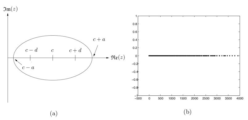
Figure 1: (a) A schematic ellipse in the complex plane with center $c$, focal distance $d$, and semi-major axis $a$.(b) Eigenvalue distribution of the test matrix bcsstm27.

An explicit expression of $C_{j}(\frac{a}{d})/C_{j}(\frac{c}{d})$ can be found on p. 207 of [34], and under some additional assumptions on $E(c,d,a)$ (say, the ellipse in Fig. 1(a)),

$$\frac{C_{j}(\frac{a}{d})}{C_{j}(\frac{c}{d})}\approx\left(\frac{a+\sqrt{a^{2}-d^{2}}}{c+\sqrt{c^{2}-d^{2}}}\right)^{j}\equiv\delta^{j}.$$ (8)

The upper bound in (7) therefore contains two factors: the condition number $\kappa_{2}(V)$ of the eigenvector matrix $V$ and the scalar $\delta$ determined by the distribution of the eigenvalues of $A$. If $A$ is nearly normal and has a spectrum $\sigma(A)$ which is clustered around $1$, we would have $\kappa_{2}(V)\approx 1$ and $\delta<1$. In this case, $\|r_{j}\|_{2}$ decays exponentially in a rate of power $\delta^{j}$, resulting in a fast convergence of GMRES. The error bound (7) hides the fact that the convergence rate is better if the eigenvalues of $A$ are clustered [42].

Since the ellipse $E(c,d,a)$ in Theorem 1 must include all of the eigenvalues of $A$, the outlying eigenvalues may keep the ellipse large, implying a large $\delta$. To reduce $\delta$, we therefore only remove these outlying eigenvalues from $\sigma(A)$. Any procedure of doing so is known as deflation. GMRES in combination with deflation is called Deflated GMRES.

0.2.2 Deflated GMRES

Suppose $x^{*}$ is the exact solution of (5). Let a so-called deflation-subspace matrix $Z=[z_{1},\ldots,z_{m}]\in{\mathbb{C}}^{N\times m}$ be given, whose columns are linearly independent. Define the two projectors [8, 21, 43, 45]

$$\begin{array}[]{rcl}P\equiv I-AZM^{-1}Z^{H}&\mbox{and}&\widetilde{P}\equiv I-ZM^{-1}Z^{H}A,\end{array}$$ (9)

where $M=Z^{H}AZ$ is assumed to be invertible. It is straightforward to verify that $P^{2}=P,\;\widetilde{P}^{2}=\widetilde{P}$ and $PA=A\widetilde{P}$.

Using $\widetilde{P}$, we split $x^{*}$ into two parts:

$$x^{*}=(I-\widetilde{P})x^{*}+\widetilde{P}x^{*}\equiv x^{*}_{1}+x^{*}_{2}.$$

For $x^{*}_{1}$, we have

$$x^{*}_{1}=(I-\widetilde{P})x^{*}=ZM^{-1}Z^{H}Ax^{*}=ZM^{-1}Z^{H}b.$$

For $x^{*}_{2}$, we obtain

$$x^{*}_{2}=A^{-1}Pb,$$

since $Ax^{*}_{2}=A\widetilde{P}x^{*}=PAx^{*}=Pb.$ Now, if $x^{\#}$ is a solution of the singular system

$$PAx=Pb,$$ (10)

then

$$\begin{array}[]{rcl}A\widetilde{P}x^{\#}=Pb&\Leftrightarrow&\widetilde{P}x^{\#}=A^{-1}Pb=x^{*}_{2}.\end{array}$$

Based on the above observation, a Deflated GMRES algorithm for the solution of (5) is given in Algorithm 1.

1.	Choose $Z$;
2.	Compute $x_{1}=ZM^{-1}Z^{H}b$;
3.	Solve $PAx=Pb$ by GMRES to obtain a solution $x^{\#}$;
4.	Compute $x_{2}=\widetilde{P}x^{\#}$;
5.	Compute $x=x_{1}+x_{2}$.

Algorithm 1 Deflated GMRES

We remark that the GMRES in Algorithm 1 can be replaced by any other linear solvers, direct or iterative. We note that when $A$ is symmetric, indefinite that we can use the MINRES method [31] instead of GMRES and compute the same solution $x$ using far less memory.

Assume that the nonsingular $A\in{\mathbb{C}}^{N\times N}$ has a decomposition (6) with $V=[v_{1},\ldots,v_{N}]$ and $\Lambda=\mbox{diag}\{\lambda_{1},\ldots,\lambda_{N}\}$. If we set $Z=[v_{1},\ldots,v_{m}]$ in (9), then the spectrum $\sigma(PA)$ contains all the eigenvalues of $A$ except $\lambda_{1},\ldots,\lambda_{m}$, namely, $\sigma(PA)=\{0,\cdots,0,\lambda_{m+1},\cdots,\lambda_{N}\}$.

Perform a $QR$ factorization on $V$ as follows:

$$V=QR\equiv[Q_{1},Q_{2}]\left[\begin{array}[]{cc}R_{11}&R_{12}\\ 0&R_{22}\end{array}\right],$$

where $Q_{1}\in{\mathbb{C}}^{N\times m}$ and $R_{11}\in{\mathbb{C}}^{m\times m}$. If we set $Z=[v_{1},\ldots,v_{m}]$ and apply GMRES to solve (10), an upper bound on $\|r_{j}\|$ is given by the following theorem [45].

Theorem 2.

Suppose that $A$ has a decomposition (6) and GMRES is used to solve (10) with $Z=[v_{1},\ldots,v_{m}]$. If all the eigenvalues $\lambda_{m+1},\ldots,\lambda_{N}$ of $A$ are located in an ellipse $E(c,d,a)$ that excludes the origin of the complex plane, then

$$\|r_{j}\|_{2}\leq\kappa_{2}(R_{22})\frac{C_{j}(\frac{a}{d})}{|C_{j}(\frac{c}{d})|}\|r_{0}\|_{2}.$$ (11)

With (8), the upper bound (11) of the residual norm $\|r_{j}\|_{2}$ of GMRES is determined by the condition number of $R_{22}$ (rather than $V$) and the scalar $\delta$ which is determined by the distribution of the undeflated eigenvalues $\lambda_{m+1},\ldots,\lambda_{N}$ of $A$. The $\delta$ in Theorem 2 is generally less than the $\delta$ associated with Theorem 1. This partially explains why an eigenvalue-deflation is likely to lead to a faster convergence of GMRES.

The proof of Theorem 2 is based on the observation that when GMRES solves a singular linear system it is actually solving a nonsingular linear system of smaller size. Theorem 2 then follows from the application of Theorem 1 to the nonsingular linear system. See [45] for the details of the proof of Theorem 2.

0.2.3 Spectral Projector and Construction of $Z$

A spectral projector is described in detail in §3.1.3-§3.1.4 of [35]. Other references include [6, 17, 27]. Let $A=VJV^{-1}$ be the Jordan canonical decomposition of $A$, where

$$\begin{array}[]{ccc}V=[v_{1},v_{2},\ldots,v_{N}]&\mbox{and}&J=diag\{J_{N_{1}}(\lambda_{1}),J_{N_{2}}(\lambda_{2}),\ldots,J_{N_{d}}(\lambda_{d})\}.\end{array}$$

The diagonal block $J_{N_{i}}(\lambda_{i})$ in $J$ is an $N_{i}\times N_{i}$ Jordan block associated with the eigenvalue $\lambda_{i}$. The eigenvalues $\lambda_{i}$ are not necessarily distinct and can be repeated according to their multiplicities.

Let $\Gamma$ be a given positively oriented simple closed curve in the complex plane. Without loss of generality, let the set of eigenvalues of $A$ enclosed by $\Gamma$ be $\{\lambda_{1},\lambda_{2},\ldots,\lambda_{k}\}$ so that the eigenvalues $\lambda_{k+1},\ldots,\lambda_{d}$ lie outside the region enclosed by $\Gamma$. Set $s\equiv N_{1}+N_{2}+\ldots+N_{k}$, the number of eigenvalues inside $\Gamma$ with multiplicity taken into account. Then the residue

$$P_{\Gamma}=\frac{1}{2\pi\sqrt{-1}}\oint_{\Gamma}(zI-A)^{-1}dz$$

defines a projection operator onto the space $\sum_{i=1}^{k}\mbox{Null}(A-\lambda_{i}I)^{l_{i}}$, where $l_{i}$ is the index of $\lambda_{i}$, namely,

$$\mbox{Range}(P_{\Gamma})=\mbox{span}\{v_{1},v_{2},\ldots,v_{s}\}.$$

In particular, if $A$ has a diagonal decomposition (6), $P_{\Gamma}$ is a projector onto the sum $\sum_{i=1}^{k}{\mathbb{E}}_{\lambda_{i}}$ of the $\lambda_{i}$-eigenspace ${\mathbb{E}}_{\lambda_{i}}$ of $A$.

Pick a random matrix $Y\in{\mathbb{C}}^{N\times m}$ and set

$$Z=P_{\Gamma}Y=\frac{1}{2\pi\sqrt{-1}}\oint_{\Gamma}(zI-A)^{-1}Ydz$$ (12)

in (9). In the case where $m=s$, we almost surely have $\sigma(PA)=\{0,\cdots,0,\lambda_{k+1},\cdots,\lambda_{d}\}$. Therefore all the eigenvalues of $A$ inside $\Gamma$ are removed from the spectrum of $PA$.

0.3 Numerical Examples

In this section, we demonstrate the effect of the deflation-subspace matrix $Z$ defined by (12) and computed by the Legendre-Gauss quadrature on the solution of the linear system (5).

All the computations were done in Matlab Version 7.1 on a Windows 10 machine. Besides GMRES, we also employ a modified BiCG (MBiCG) as the Krylov solver in Line 3 of Algorithm 1 and for finding the solution of all of the linear systems in the computation of $Z$. The MBiCG is the standard BiCG, but outputs the computed solution $x$ that either satisfies relres $<$ tol or has the smallest relative residue among all the computed $x$ from iteration $1$ to iteration maxit, where relres is the relative residue of $x$, tol is the user supplied input stopping tolerance, and maxit is the maximum number of iterations.

The numerical solution using a deflated, restarted GMRES of the linear systems obtained from the discretization of the two dimensional steady-state convection-diffusion equation

$$\begin{array}[]{rcl}-u_{xx}-u_{yy}-Re\,(p(x,y)u_{x}-q(x,y)u_{y})]=f(x,y),&&(x,y)\in[0,1]^{2}\end{array}$$ (13)

with Dirichlet boundary conditions was studied in depth in [8]. This steady-state version (13) of the two-dimensional convection-diffusion equation is from [47].

In [8], two types of deflation-subspace matrices $Z$ were used: eigenvectors obtained from the Matlab function $eig$ and algebraic subdomain vectors. The $Z$ of algebraic subdomain vectors works well for the fluid flow problem (13), but seems not for the other problem presented in [8]. Accurately calculating eigenvalues of large matrices is very time consuming. Therefore deflation with the $Z$ of true eigenvectors is not practicable.

Numerical experiments in [8] have shown that eigenvalues close to the origin hamper the convergence of a Krylov subspace method. Hence, deflation of these eigenvalues is very beneficial. Based on this observation, we chose in our experiments the integration path $\Gamma$ in (12) to be a circle $D(c,r)$ with the center $c$ near the origin. For the $Y$ in (12), we picked a random $Y\in{\mathbb{R}}^{N\times m}$ by the Matlab command $Y=randn(N,m)$ with $m$ not less than the exact number $s$ of eigenvalues inside $\Gamma$. We remark that an efficient stochastic estimation method of $s$ has been developed in [22].

We computed the integral in (12) by the Legendre-Gauss quadrature

$$Z=\frac{r}{2}\int_{-1}^{1}e^{\pi\theta i}((c+re^{\pi\theta i})I-A)^{-1}Yd\theta\approx\frac{r}{2}\sum_{k=1}^{q}\omega_{k}e^{\pi\theta_{k}i}((c+re^{\pi\theta_{k}i})I-A)^{-1}Y,$$ (14)

where $i=\sqrt{-1}$, and $\omega_{k}$ and $\theta_{k}$ are the Legendre-Gauss weights and nodes on the interval $[-1,1]$ with truncation order $q$.

In (14), there are $mq$ linear systems

$$\begin{array}[]{rccl}((c+re^{\pi\theta_{k}\sqrt{-1}})I-A)x=y_{j},&&k=1,\ldots,q,&j=1,\ldots,m\end{array}$$ (15)

to solve. We solved all of them by GMRES or MBiCG with the stopping tolerance $tol=10^{-15}$ and the maximum number of iterations $maxit=500$ or $1000$.

Mathematically, the rank of $Z$ defined by (12) is less than $m$ when $m>s$. As a result, the matrix $M$ in (9) is singular. In practice, $Z$ is approximated by (14) and the matrix $M$ becomes near-singular. In order to remedy this difficulty, one can use the singular value decomposition (SVD) or the QR decomposition of $Z$ to detect and remove its nearly dependent columns. The SVD or QR decomposition involves a high communication cost and may not be favorable for a parallel computation. In this paper, we suggest a column deflation mechanism based on Gaussian elimination (GE) with complete pivoting [23] to remove the dependent columns in $Z$.

The rationale of the mechanism is as follows. Let $\widehat{Z}=Z^{H}Z\in{\mathbb{C}}^{m\times m}$. It can be seen that $rank(Z)=rank(\widehat{Z})$. We perform GE with complete pivoting on $\widehat{Z}$ to reduce $\widehat{Z}$ into an upper triangular form. Accordingly, we interchange the corresponding columns in $Z$. If at some step of $j$ the lower right block $\widehat{Z}_{(j+1:m,j+1:m)}=0$, then the rank of $\widehat{Z}$ is $j$ and $Z_{(:,1:j)}$ consists of all the linearly independent columns of $Z$. The purpose that we left-multiply $Z$ by $Z^{H}$ to form $\widehat{Z}$ is (i) to reduce the row size of $Z$ from $N$ to $m$, and (ii) to reduce data movements in the GE process. See Algorithm 2 in §0.6 for implementation details.

In our experiments, we performed the following eight computations. Numerical results are summarized in Tables 1-7.

1. Solve (5) by GMRES (or MBiCG) with the initial guess $x=0$ with $tol=10^{-7}$ and $maxit=10^{3}N$. Compute the true relative errors relres2 $=\|b-Ax\|_{2}/\|b\|_{2}$ and relerr $=\|x-x^{*}\|_{2}/\|x^{*}\|_{2}$, where $x$ is the computed solution output by GMRES (or MBiCG) and $x^{*}$ is the exact solution of (5).

2. Compute by the Matlab function eig the eigenvectors $v_{1},\ldots,v_{s}$ of $A$ whose associated eigenvalues lie inside $\Gamma$. Set $Z=[v_{1},\ldots,v_{s}]$. Perform Algorithm 1 with GMRES (or MBiCG) as its linear solver (see Line 3 of Algorithm 1). Set the initial guess $x=0$ with $tol=10^{-7}$ and $maxit=10N$ for GMRES (or MBiCG). Compute the true relative errors relres1 $=\|Pb-PAx^{\#}\|_{2}/\|Pb\|_{2}$, relres2 $=\|b-Ax\|_{2}/\|b\|_{2}$, and relerr $=\|x-x^{*}\|_{2}/\|x^{*}\|_{2}$, where $x^{\#}$ and $x$ are the computed solutions in Lines 3 and 5 of Algorithm 1, respectively.

3. Solve all the linear systems in (15) by GMRES (or MBiCG) with the initial guess $x=0$ with $tol=10^{-15}$ and $maxit=500$. Compute $Z$ using (14). Perform Algorithm 1 with the initial guess $x=0$ with $tol=10^{-7}$ and $maxit=10N$ for GMRES (or MBiCG). Compute the true relative errors relres1, relres2, and relerr defined in item #2.

4. Perform the same computations as described in item #3 with $maxit=1000$ instead of $maxit=500$.

5. Solve all the linear systems in (15) by GMRES (or MBiCG) with the initial guess $x=0$ with $tol=10^{-15}$ and $maxit=500$. Compute $Z$ using (14). Setting $\alpha=10^{-8}$ and $tol\_cge=10^{-2}$, perform Algorithm 2 on the computed $Z$ to remove its nearly dependent columns. Using the $Z$ output from Algorithm 2, perform Algorithm 1 with the initial guess $x=0$ with $tol=10^{-7}$ and $maxit=10N$ for GMRES (or MBiCG). Compute the true relative errors relres1, relres2, and relerr defined in item #2.

6. Perform the same computations as described in item #5 with $maxit=1000$ instead of $maxit=500$.

7. Solve all the linear systems in (15) by GMRES (or MBiCG) with the random initial guess $x=randn(N,1)$ with $tol=10^{-15}$, and $maxit=500$. Compute $Z$ through (14). Perform Algorithm 1 with the initial guess $x=0$ with $tol=10^{-7}$, and $maxit=10N$ for GMRES (or MBiCG). Compute the true relative errors relres1, relres2, and relerr defined in item #2.

8. Perform the same computations as described in item #7 with $maxit=1000$ instead of $maxit=500$.

0.3.1 Example 1

As in [8], consider the convection-diffusion equation (13) with Dirichlet boundary conditions. The convection coefficients $p(x,y)$, $q(x,y)$, and the source term $f(x,y)$ were chosen as

$$\begin{array}[]{l}p(x,y)=-\sin x\cos\pi y\\ q(x,y)=\cos(\pi x)\sin y,\\ f(x,y)=52\sin(4x+6y)-(4p(x,y)-6q(x,y))\cos(4x+6y).\end{array}$$

Equation (13) was discretized on the unit square $[0,1]^{2}$ using a $5$-point central difference scheme with a uniform mesh size of $h=1/100$ with resulting linear systems (5) of size $N=99^{2}$.

The Reynolds number $Re$ controls the degree of the nonsymmetry in the coefficient matrix $A$ of (5). When $Re=0$, $A$ is symmetric. As $Re$ increases the nonsymmetry in $A$ also increases.

In our experiments, we pick the coefficient matrix $A$, but set the right hand side $b=A{\bf 1}$, where ${\bf 1}=[1,1,\ldots,1]^{T}$. We know a priori the exact solution of (5) and the relative error relerr is computable. We choose $Re=8000$. The integration path $\Gamma$ is the circle whose center is the origin and has radius $0.5$. Figure 2 presents the eigenvalue distribution of $A$.

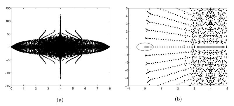
Figure 2: (Example 1) (a) Eigenvalue distribution of the test matrix $A$. (b) Eight eigenvalues of $A$ lie inside $\Gamma$, the circle centered at the origin with radius $0.5$. The eigenvalue with the smallest distance to the origin is $4.3e\!-\!3$.

Comparing the numerical results of Computations #1 and #2 in Table 1, we see that the convergence of GMRES can be made much faster with an appropriate eigenvalue-deflation. Specifically GMRES takes $3295$ iterations to solve (5), but only $1815$ iterations to solve (10). This experiment supports the observation made in [8] that eigenvalues close to the origin hamper the convergence of a Krylov subspace method. It also supports the theory presented in §0.2.2.

The behavior of a Krylov subspace method on the solution of (10) depends on (i) the quality of the approximation of the computed $Z$ to the exact eigenvectors, (ii) the column size $m$ of $Z$, (iii) the condition of $M$, and (iv) perhaps some other unknown factors.

Consider the computed $Z$’s in Tables 2 and 3. Comparing the corresponding relative residue ranges in the second columns of the tables we see that the $Z$’s in Table 3 are closer to the exact eigenvectors than the $Z$’s in Table 2 are since the range intervals in Table 3 are closer to the origin $0$. As a result, the GMRES and MBiCG results in Table 3 converge faster than those in Table 2 when solving (10).

Consider Table 3. As $m$ is increases from $10$ to $50$, the condition numbers Cd($M$) of $M$ does not increase substantially. In this case, the number of iterations needed by GMRES and MBiCG to converge decreases (see the 5th column of the table).

In Example 1, the exact number $s$ of eigenvalues of $A$ inside the circle $\Gamma$ is $8$. The rank of $Z$ in (12) is $8$ mathematically and therefore the $2$-norm condition number of $Z$ is $\infty$ in the case when $m>s$. However, the condition numbers of the computed $Z$’s in Tables 2 and 3 are small finite numbers. This implies that those computed $Z$’s are inaccurate. They only contain partial information about the true eigenvectors. Impressively, the computed $Z$’s in Table 3 associated with $m=50$ perform even better than the true eigenvectors do (compare the 4th column in Table 1 and the 5th column in Table 3).

Since the computed $Z$’s in Example 1 perform so well, there is no reason to apply Algorithm 2 to improve their conditions.

Computation #1			Computation #2
Solve (5) by GMRES			Solve (10) by GMRES		Algorithm 1
#iter	relres2	relerr	#iter	relres1	relres2	relerr
$3295$	$9.9e\!-\!8$	$3.3e\!-\!7$	$1815$	$9.9e\!-\!8$	$9.9e\!-\!8$	$3.4e\!-\!6$
Solve (5) by MBiCG			Solve (10) by MBiCG		Algorithm 1
#iter	relres2	relerr	#iter	relres1	relres2	relerr
$10125$	$9.5e\!-\!8$	$2.7e\!-\!8$	$3951$	$9.9e\!-\!8$	$9.9e\!-\!8$	$2.2e\!-\!8$

Table 1: (Example 1) $\Gamma$ is the circle centered at the origin with radius $0.5$. The number of eigenvalues of $A$ inside $\Gamma$ is $8$. #iter stands for the number of iterations needed to converge.

Computation #3
Solve (15) by GMRES		Compute $Z$ by (14)		Solve (10) by GMRES		Algorithm 1
$m$	Rel. Res. Range	Cd($Z$)	Cd($M$)	#iter	relres1	relres2	relerr
$10$	$[1.4e\!-\!3,1.1e\!-\!1]$	$6.7$	$1.8e\!+\!1$	$2616$	$9.9e\!-\!8$	$1.0e\!-\!7$	$1.9e\!-\!6$
$50$	$[1.1e\!-\!3,1.2e\!-\!1]$	$4.5e\!+\!1$	$3.0e\!+\!2$	$1321$	$9.9e\!-\!8$	$9.9e\!-\!8$	$9.2e\!-\!7$
Solve (15) by MBiCG		Compute $Z$ by (14)		Solve (10) by MBiCG		Algorithm 1
$m$	Rel. Res. Range	Cd($Z$)	Cd($M$)	#iter	relres1	relres2	relerr
$10$	$[2.6e\!-\!2,5.5e\!-\!1]$	$5.9e\!+\!2$	$1.8e\!+\!4$	$6875$	$6.8e\!-\!8$	$8.4e\!-\!8$	$6.2e\!-\!8$
$50$	$[2.3e\!-\!2,5.2e\!-\!1]$	$3.0e\!+\!6$	$6.7e\!+\!10$	$6078$	$9.9e\!-\!8$	$1.4e\!-\!7$	$3.1e\!-\!7$

Table 2: (Example 1) The integration path $\Gamma$ is the same as in Table 1. The $q$ in (14) was set to be $q=2^{4}$. After each of the linear systems in (15) was solved, the true relative residue $\|y_{j}-((c+re^{\pi\theta_{k}\sqrt{-1}})I-A)x\|_{2}/\|y_{j}\|_{2}$ of the approximate solution $x$ was computed. The intervals in the column titled “Rel. Res. Range” are the smallest intervals that contain these relative residues. Cd$(Z)$ and Cd$(M)$ stand for the $2$-norm condition numbers of $Z$ and $M$ respectively.

Computation #4
Solve (15) by GMRES		Compute $Z$ by (14)		Solve (10) by GMRES		Algorithm 1
$m$	Rel. Res. Range	Cd($Z$)	Cd($M$)	#iter	relres1	relres2	relerr
$10$	$[4.1e\!-\!6,6.0e\!-\!2]$	$1.1e\!+\!1$	$8.0e\!+\!1$	$2420$	$9.9e\!-\!8$	$9.9e\!-\!8$	$2.4e\!-\!6$
$50$	$[3.0e\!-\!6,8.5e\!-\!2]$	$1.3e\!+\!2$	$1.9e\!+\!3$	$1340$	$9.9e\!-\!8$	$9.9e\!-\!8$	$1.8e\!-\!6$
Solve (15) by MBiCG		Compute $Z$ by (14)		Solve (10) by MBiCG		Algorithm 1
$m$	Rel. Res. Range	Cd($Z$)	Cd($M$)	#iter	relres1	relres2	relerr
$10$	$[9.9e\!-\!4,5.8e\!-\!1]$	$9.6$	$3.3e\!+\!1$	$6081$	$9.3e\!-\!8$	$1.1e\!-\!7$	$5.8e\!-\!8$
$50$	$[1.1e\!-\!3,5.2e\!-\!1]$	$8.7e\!+\!1$	$9.5e\!+\!2$	$2621$	$9.8e\!-\!8$	$1.1e\!-\!7$	$1.5e\!-\!7$

Table 3: (Example 1) The integration path $\Gamma$ is the same as in Table 1, and $q=2^{4}$ in (14). For the meanings of the columns, refer to Tables 1 and 2.

0.3.2 Example 2

The following two test data sets are part of The University of Florida Sparse Matrix Collection [7]. These data sets have been used in [9] for the numerical experiments.

1. bcsstm27 is from a mass matrix buckling problem. It is a $1224\times 1224$ real symmetric and indefinite matrix $A$ with $56126$ nonzero entries. Per the right hand side in (5), we set $b=A{\bf 1}$, where ${\bf 1}$ is the vector of all ones. A spectral plot for bcsstm27 is presented in Figure 1(b).

2. mahindas is from an economics problem. It is a $1258\times 1258$ real unsymmetric matrix $A$ with $7682$ nonzero entries. Again, we set $b=A{\bf 1}$ as the right hand side in (5). A spectral plot for mahindas is in Figure 3(a).

An ILU preconditioner generated by the Matlab function $[L,U,Pr]=luinc(A,^{\prime}0^{\prime})$ was used for mahindas, namely, instead of solving (5), we solved

The Matlab function $[L,U,Pr]=luinc(A,^{\prime}0^{\prime})$ is used to create an ILU preconditioner for mahindas. Instead of solving (5), we solved

$$\tilde{A}x=\tilde{b}$$ (16)

by Algorithm 1, where $\tilde{A}=L^{-1}PrAU^{-1}$ and $\tilde{b}=L^{-1}Prb$. The $A$ and $b$ in (10) are replaced with $\tilde{A}$ and $\tilde{b}$, respectively. Once a solution $x$ to (16) is obtained, we compute a solution to the original system (5) by $U^{-1}x$. Since the $U$ factor obtained from luinc has some zeros along its main diagonal, we replace those zeros by $1$ so that $U$ is invertible. A spectral plot for $\tilde{A}$ is given in Figure 3(b).

However, we do not apply any preconditioner to bcsstm27.

In Example 2, we only use MBiCG as the linear solver. Numerical results are summarized in Tables 4-7.

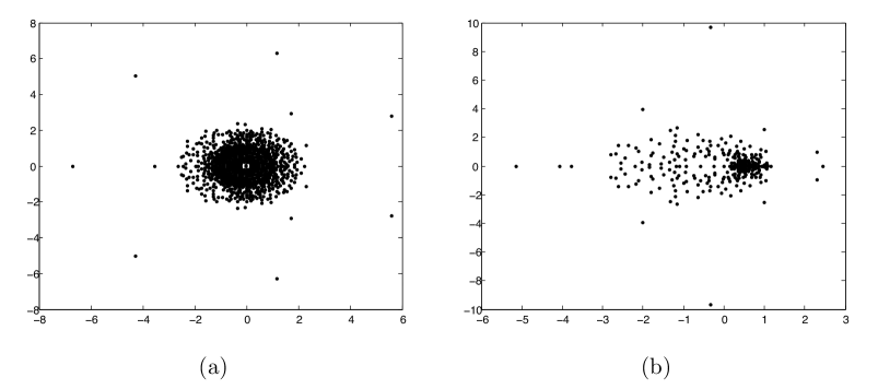
Figure 3: (a) Eigenvalue distribution of the test matrix mahindas. (b) Eigenvalue distribution of the ILU($0$)-preconditioned mahindas.

Without deflation MBiCG performs very poorly for both bcsstm27 and the ILU($0$)-preconditioned mahindas. Specifically, MBiCG does not converge within maxit $=10^{3}N$ iterations in terms of the relative residues relres2. Further, the computed solutions by MBiCG are far from the corresponding exact solutions $x^{*}={\bf 1}$ according to the relative errors relerr. With an appropriate eigenvalue-deflation, however, the situation is improved (see the numerical results in Tables 5-7).

The computed matrices $Z$ in Computations #3 and #4 in Table 5 worked well for bcsstm27, but not for the ILU($0$)-preconditioned mahindas. The computed $Z$’s for mahindas contain some nearly dependent columns that lead to large condition numbers Cd($M$) of $M$. The situation is significantly improved after the nearly dependent columns in $Z$ are removed using Algorithm 2. As a result, MBiCG converged when it solved (10) (see Table 6).

Now compare Computations #4 and #6 for bcsstm27 in Tables 5 and 6, respectively. The two condition numbers Cd($M$) of $M$ do not differ much in magnitude, but the $m$ ($=400$) in Computation #4 is larger than the $m$ ($=371$) in Computation #6. As a result, MBiCG converged faster in Computation #4 than it did in Computation #6 when solving (10).

In Computations #7 and #8, we randomly picked an initial guess for the solution of each linear system in (15) and then computed $Z$ by (14). The resulting $Z$ has a better performance than the $Z$ obtained with a zero initial guess as in Computations #3–#6. We first compare Computation #8 and Computation #4 for mahindas in Tables 7 and 5. Both condition numbers Cd($M$) of $M$ are about the same in magnitude, but MBiCG and Algorithm 1 in Computation #8 performs much better than in Computation #4.

We compare Computations #8 and #6 for mahindas in Tables 7 and 6. The column size $m$ of $Z$ in Computation #8 ($m=50$) is much larger than the $m$ in Computation #6 ($m=10$). This explains the faster convergence of MBiCG in Computation #8 on the solution of (10) despite the fact that the $M$ in Computation #8 is ill conditioned relative to the $M$ in Computation #6.

Finally, we remark that we have chosen $m\geq s$ in the experiments presented above. When $m<s$, Algorithm 1 plus (14) still works well, but not as impressively as in the case when $m\geq s$. For an estimate of $s$, the stochastic method in [22] should be useful. See [46] for a concise description of this method. Moreover, the method in [29] is also recommended.

The most expensive part in the proposed method of Algorithm 1 plus (14) is clearly the computation of $Z$ in (14). In §0.4, we describe state of the art parallel multigrid methods that can be applied to the computation of $Z$.

			Computation #1			Computation #2
	Circle $\Gamma$		Solve (5)			Solve (10)		Algorithm 1
Matrix	$(c,r)$	#eig $\Gamma$	#iter	relres2	relerr	#iter	relres1	relres2	relerr
bcsstm27	$(0,5)$	$363$	$1224000$	$2.0e\!-\!6$	$5.7e\!-\!1$	$227$	$9.5e\!-\!8$	$9.5e\!-\!8$	$2.4e\!-\!7$
mahindas	$(-1,1)$	$31$	$1258000$	$3.5e\!-\!7$	$1.8$	$1841$	$5.6e\!-\!8$	$5.6e\!-\!8$	$4.4e\!-\!3$

Table 4: (Example 2) The linear systems (5) and (10) were solved by MBiCG. $\Gamma$ is a circle with center $c$ and radius $r$. #eig $\Gamma$ stands for the number of eigenvalues of $A$ inside $\Gamma$, and #iter the number of iterations by MBiCG. For mahindas, an ILU($0$) preconditioner was applied.

Computation #3
	Solve (15)		Compute $Z$ by (14)		Solve (10)		Algorithm 1
Matrix	$m$	Rel. Res. Range	Cd($Z$)	Cd($M$)	#iter	relres1	relres2	relerr
bcsstm27	$400$	$[4.1e\!-\!10,6.1e\!-\!2]$	$1.5e\!+\!3$	$1.0e\!+\!6$	$843$	$6.3e\!-\!8$	$6.2e\!-\!8$	$5.0e\!-\!6$
mahindas	$50$	$[1.2e\!-\!10,1.0]$	$1.3e\!+\!2$	$1.7e\!+\!6$	$12580$	$6.4e\!-\!2$	$2.2e\!-\!1$	$2.5e\!+\!4$
Computation #4
bcsstm27	$400$	$[3.2e\!-\!14,8.0e\!-\!4]$	$2.5e\!+\!3$	$4.5e\!+\!6$	$563$	$9.2e\!-\!8$	$9.2e\!-\!8$	$3.4e\!-\!2$
mahindas	$50$	$[1.5e\!-\!10,1.0]$	$2.5e\!+\!2$	$2.2e\!+\!6$	$12580$	$3.1e\!-\!2$	$3.6e\!-\!2$	$1.3e\!+\!4$

Table 5: (Example 2) The integration paths $\Gamma$ are shown in Table 4, and $q=2^{4}$ in (14). The linear systems (15) and (10) were solved by MBiCG. For the meanings of the columns, refer to Tables 1 and 2.

Computation #5
	Solve (15)		Algorithm 2			Solve (10)		Algorithm 1
Matrix	$m$	Rel. Res. Range	rk of $Z$	Cd($Z$)	Cd($M$)	#iter	relres1	relres2	relerr
bcsstm27	$400$	$[4.1e\!-\!10,6.1e\!-\!2]$	$370$	$9.3e\!+\!1$	$1.2e\!+\!5$	$2824$	$8.8e\!-\!8$	$8.8e\!-\!8$	$6.2e\!-\!2$
mahindas	$50$	$[1.2e\!-\!10,1.0]$	$12$	$2.7e\!+\!1$	$8.9e\!+\!2$	$9318$	$8.6e\!-\!8$	$8.6e\!-\!8$	$6.0e\!-\!3$
Computation #6
bcsstm27	$400$	$[3.2e\!-\!14,8.0e\!-\!4]$	$371$	$9.4e\!+\!1$	$1.9e\!+\!5$	$2224$	$5.8e\!-\!8$	$5.8e\!-\!8$	$6.3e\!-\!2$
mahindas	$50$	$[1.5e\!-\!10,1.0]$	$10$	$1.9e\!+\!1$	$4.4e\!+\!2$	$4688$	$6.8e\!-\!8$	$6.8e\!-\!8$	$3.5e\!-\!3$

Table 6: (Example 2) The integration paths $\Gamma$ are shown in Table 4, and $q=2^{4}$ in (14). The linear systems (15) and (10) were solved by MBiCG. The numbers in the column titled “rk of $Z$” are the numerical ranks rk of $Z$ output by Algorithm 2. For the meanings of other columns, refer to Tables 1 and 2.

Computation #7
	Solve (15)		Compute $Z$ by (14)		Solve (10)		Algorithm 1
Matrix	$m$	Rel. Res. Range	Cd($Z$)	Cd($M$)	#iter	relres1	relres2	relerr
bcsstm27	$400$	$[3.9e\!-\!9,2.2e\!-\!1]$	$5.8e\!+\!2$	$5.4e\!+\!5$	$1114$	$8.2e\!-\!8$	$8.4e\!-\!8$	$1.9e\!-\!6$
mahindas	$50$	$[2.8e\!-\!10,2.0e\!+1]$	$8.5e\!+\!1$	$1.2e\!+\!5$	$12580$	$5.6e\!-\!5$	$5.7e\!-\!5$	$4.8$
Computation #8
bcsstm27	$400$	$[2.7e\!-\!13,3.1e\!-\!3]$	$2.3e\!+\!3$	$4.3e\!+\!6$	$686$	$9.1e\!-\!8$	$9.1e\!-\!8$	$3.2e\!-\!6$
mahindas	$50$	$[9.8e\!-\!11,1.3e\!+\!1]$	$6.7e\!+\!2$	$9.7e\!+\!6$	$2286$	$8.4e\!-\!8$	$8.5e\!-\!8$	$1.8e\!-\!2$

Table 7: (Example 2) The integration paths $\Gamma$ are shown in Table 4, and $q=2^{4}$ in (14). The linear systems (15) and (10) were solved by MBiCG. For the meanings of the columns, refer to Tables 1 and 2.

0.4 Future Work

We can formulate either geometric multigrid [1, 2, 5, 11, 19, 20, 26, 44] or algebraic multigrid [39] using the same notation level to level using the abstract multigrid approach developed in [10, 13, 15, 3, 12, 13, 15].

Assuming the cost of the smoother (or rougher) on each level is $O(N_{j})$, $j=1,\cdots,k$, Algorithm MGC with $p$ recursions to solve problems on level $k-1$ has complexity

$$W_{MGC}(N_{k})=\left\{\begin{array}[]{ll}O(N_{k})&1\leq p\leq\sigma\\ O(N_{k}\log N_{k})&p=\sigma\\ O(N_{k}^{\log p})&p>\sigma.\\ \end{array}\right.$$

Under the right circumstances, multigrid is of optimal order as a solver.

Consider the example (13) in §0.3. A simple geometric multigrid approximation to (13) produces a very good solution in $4$ V Cycles or $2$ W cycles using the deflated GMRES as the rougher. Each V or W Cycle is $O(N_{k})$. Hence, we have an optimal order solver for (13), which would not be the case if we used BiCG or deflated GMRES on a single grid.

High performance computing versions of multigrid based on using hardware acceleration with memory caches was extensively studied in the early 2000’s [16].

Parallelization of Algorithm MGC is straightforward [14].

• For geometric multigrid, on each level $j$, data is split using a domain decomposition paradigm. Parallel smoothers (roughers) are used. The convergence rate degrades from the standard serial theoretical rate, but not by a lot, and scaling is good given sufficient data.

• For algebraic multigrid, the algorithms can be either straightforward (e.g., Ruge-Studen [33] or Beck [4]) to quite complicated (e.g., AMGe [25]). Solutions have existed for a number of years, so it is a matter of choosing an exisiting implementation. In some cases, using a tool like METIS or ParMETIS is sufficient to create a domain decomposition-like system based on graph connections in $A_{j}$, which reduces parallelization back to something similar to the geometric case.

In many cases, the complexity of this type of parallel multigrid for $P$ processors becomes

$$W_{MGC,P}(N_{k})=W_{MGC}(N_{k})\log P/P.$$

0.5 Conclusions

We incorporate the delation projector $P$ in (9), with $Z$ defined by and computed by (12) and (14), respectively, into Krylov subspace methods to enhance the stability and accelerate the convergence of the iterative methods for solving ill conditioned linear systems. Our experiments suggest that Algorithm 1 plus (14) has the potential to solve ill conditioned problems much faster and more accurately than standard Krylov subspace solvers. Moreover, to our best knowledge, the constructions of most, if not all, deflation subspace matrices $Z$ in the literature are problem dependent. The method proposed here, however, is problem independent.

More experiments, especially on test data of large size (e.g., millions or more unknowns) are needed to better understand the behavior of the proposed algorithm. Implementation of robust and efficient parallel multigrid methods for solving (15) and the realization of a software package for a wide variety of applications is currently under our investigation.

0.6 Appendix

The following Algorithm 2 employs the Gaussian elimination with complete pivoting (CGE) to detect the rank rk and to select linearly independent columns of an input $Z\in{\mathbb{C}}^{N\times m}$, where $\alpha$ is a comparison parameter and tol_cge is a stopping tolerance. The output $Z$ of the algorithm is a $N$-by-$rk$ matrix consisting of the selected columns of the input $Z$.

Function $[Z,rk]=\mbox{cge}(Z,\alpha,tol\_cge)$
1.	Form $\widehat{Z}=Z^{H}Z\in{\mathbb{C}}^{m\times m}$; Set $rk=m$.
2.	Determine $(i_{0},j_{0})$ with $1\leq i_{0},j_{0}\leq m$ so that
			$|\widehat{Z}_{i_{0}j_{0}}|=\max\{|\widehat{Z}_{ij}|:1\leq i,j\leq m\}$.
3.	If $|\widehat{Z}_{i_{0}j_{0}}|<\alpha$, then set $rk=0$ and $Z=[\,\,]$; Stop.
4.	Set $\alpha=|\widehat{Z}_{i_{0}j_{0}}|$;
5.	$\widehat{Z}_{(:,1)}\leftrightarrow\widehat{Z}_{(:,j_{0})}$; $\widehat{Z}_{(1,:)}\leftrightarrow\widehat{Z}_{(i_{0},:)}$.    % move $\widehat{Z}_{i_{0}j_{0}}$ to the $(1,1)$ position.
6.	$Z_{(:,1)}\leftrightarrow Z_{(:,j_{0})}$.   % interchange the $1$st and the $j_{0}$th columns of $Z$.
7.	For $j=1:m-1$
8.		For $i=j+1:m$
9.			$\widehat{Z}_{(i,j:m)}=\widehat{Z}_{(i,j:m)}-(\widehat{Z}_{ij}/\widehat{Z}_{jj})\widehat{Z}_{(j,j:m)}$.    % perform elimination.
10.		End
11.		Determine $(i_{0},j_{0})$ with $j+1\leq i_{0},j_{0}\leq m$ so that
				$|\widehat{Z}_{i_{0}j_{0}}|=\max\{|\widehat{Z}_{pq}|:j+1\leq p,q\leq m\}$.
12.		If $|\widehat{Z}_{i_{0}j_{0}}|/\alpha<tol\_cge$, set $rk=j$ and $Z=Z_{(:,1:rk)}$; Stop.
13.		$\widehat{Z}_{(:,j+1)}\leftrightarrow\widehat{Z}_{(:,j_{0})}$; $\widehat{Z}_{(j+1,:)}\leftrightarrow\widehat{Z}_{(i_{0},:)}$.   % move $\widehat{Z}_{i_{0}j_{0}}$ to the $(j+1,j+1)$ position.
14.		$Z_{(:,j+1)}\leftrightarrow Z_{(:,j_{0})}$.   % interchange column $j_{0}$ and column $j+1$ of $Z$.
15.	End

Algorithm 2 Gaussian elimination with complete pivoting to detect the rank and to select linearly independent columns of an input matrix $Z$.

In Line 3 of Algorithm 2, we consider $\widehat{Z}=0$ when $|\widehat{Z}_{i_{0}j_{0}}|$ is small compared to $\alpha$, and hence the rank rk of $Z$ is zero. Similarly, in Line 12, if $|\widehat{Z}_{i_{0}j_{0}}|$ is small compared to $\alpha$, then we regard $\widehat{Z}_{(j+1:m,j+1:m)}$ as $0$, and therefore $rk=j$.

References

- [1] G. P. Astrakhantsev. An iterative method of solving elliptic net problems. Z. Vycisl. Mat. i. Mat. Fiz., 11:439–448, 1971.
- [2] N. S. Bakhvalov. On the convergence of a relaxation method under natural constraints on an elliptic operator. Z. Vycisl. Mat. i. Mat. Fiz., 6:861–883, 1966.
- [3] R. E. Bank and C. C. Douglas. Sharp estimates for multigrid rates of convergence with general smoothing and acceleration. SIAM J. Numer. Anal., 22:617–633, 1985.
- [4] R. Beck. Graph-based algebraic multigrid for lagrange-type finite elements on simplicial meshes. Preprint SC 99-22, Konrad-Zuse-Zentrum fur Informationstechnik, 1999.
- [5] A. Brandt. Multi–level adaptive solutions to boundary–value problems. Math. Comp., 31:333–390, 1977.
- [6] F. Chatelin. Spectral Approximation of Linear Operators. Academic Press, New York, 1984.
- [7] Tim A. Davis and Yifan Hu. The university of florida sparse matrix collection. ACM Transactions on Mathematical Software, 38:1–25, 2011. http://www.cise.ufl.edu/research/sparse/matrices (last visited April 4, 2016).
- [8] R. M. Dinkla. GMRES() with deflation applied to nonsymmetric systems arising from fluid mechanics problems. Master’s thesis, Delft University of Technology, Delft, The Netherlands, 2009.
- [9] C. Douglas, L. Lee, and M. Yeung. On solving ill conditioned linear systems. Procedia Computer Science, 80:1–10, 2016.
- [10] C. C. Douglas. Abstract multi–grid with applications to elliptic boundary–value problems. In G. Birkhoff and A. Schoenstadt, editors, Elliptic Problem Solvers II, pages 453–466. Academic Press, New York, 1984.
- [11] C. C. Douglas. Multi–grid algorithms with applications to elliptic boundary–value problems. SIAM J. Numer. Anal., 21:236–254, 1984.
- [12] C. C. Douglas. A generalized multigrid theory in the style of standard iterative methods. In Multigrid Methods IV, Proceedings of the Fourth European Multigrid Conference, Amsterdam, July 6-9, 1993, volume 116 of ISNM, pages 19–34, Basel, 1994. Birkhäuser.
- [13] C. C. Douglas. Madpack: A family of abstract multigrid or multilevel solvers. Comput. Appl. Math., 14:3–20, 1995.
- [14] C. C. Douglas. A review of numerous parallel multigrid methods. In G. Astfalk, editor, Applications on Advanced Architecture Computers, pages 187–202. SIAM, Philadelphia, 1996.
- [15] C. C. Douglas, J. Douglas, and D. E. Fyfe. A multigrid unified theory for non-nested grids and/or quadrature. E. W. J. Numer. Math., 2:285–294, 1994.
- [16] C. C. Douglas, J. Hu, M. Kowarschik, U. Rüde, and C. Weiss. Cache optimization for structured and unstructured grid multigrid. Elect. Trans. Numer. Anal., 10:21–40, 2000.
- [17] N. Dunford and J. T. Schwartz. Linear Operators, General Theory (Part I). Wiley-Interscience, Hoboken, New Jersey, 1988.
- [18] H. W. Engl. Regularization methods for the stable solution of inverse problems. Surveys Math. Indust., 3:71–143, 1993.
- [19] R. P. Fedorenko. A relaxation method for solving elliptic difference equations. Z. Vycisl. Mat. i. Mat. Fiz., 1:922–927, 1961. Also in U.S.S.R. Comput. Math. and Math. Phys., 1 (1962), pp. 1092–1096.
- [20] R. P. Fedorenko. The speed of convergence of one iterative process. Z. Vycisl. Mat. i. Mat. Fiz., 4:559–563, 1964. Also in U.S.S.R. Comput. Math. and Math. Phys., 4 (1964), pp. 227–235.
- [21] J. Frank and C. Vuik. On the construction of deflation-based preconditioners. SIAM J. Sci. Comput., 23(2):442–462, 2001.
- [22] Y. Futamura, H. Tadano, and T. Sakurai. Parallel stochastic estimation method of eigenvalue distribution. JSIAM Letters, 2:27–30, 2011.
- [23] G. Golub and C. Van Loan. Matrix Computations. The Johns Hopkins University Press, Baltimore, 4th edition, 2013.
- [24] C. W. Groetsch. Generalized Inverses of Linear Operators. Dekker, New York, 1997.
- [25] G. Haase. A parallel AMG for overlapping and non-overlapping domain decomposition. Elect. Trans. Numer. Anal., 10:41–55, 2000.
- [26] W. Hackbusch. Multigrid Methods and Applications, volume 4 of Computational Mathematics. Springer–Verlag, Berlin, 1985.
- [27] T. Kato. Perturbation Theory for Linear Operators. Springer-Verlag, New York, 1976.
- [28] L. Mansfield. Damped Jacobi preconditioning and coarse grid deflation for conjugate gradient iteration on parallel computers. SIAM J. Sci. Stat. Comput., 12(6):1314–1323, 1997.
- [29] Edoardo Di Napoli, Eric Polizzi, and Yousef Saad. Efficient estimation of eigenvalue counts in an interval. arXiv:1308.4275, 2014.
- [30] R. A. Nicolaides. Deflation of conjugate gradients with applications to boundary value problems. SIAM J. Numer. Anal., 24:355–365, 1987.
- [31] C. C. Paige and M. A. Saunders. Solution of sparse indefinite systems of linear equations. SIAM J. Numer. Anal., 12:617–629, 1975.
- [32] E. Polizzi. Density-matrix-based algorithm for solving eigenvalue problems. Phys. Rev. B, 79, no. 115112, 2009.
- [33] J. W. Ruge and K. Stüben. Efficient solution of finite difference and finite element equations by algebraic multigrid (AMG). In D. J. Paddon and H. Holstein, editors, Multigrid Methods for Integral and Differential Equations, The Institute of Mathematics and its Applications Conference Series, pages 169–212. Clarendon Press, Oxford, 1985.
- [34] Y. Saad. Iterative Methods for Sparse Linear Systems. SIAM, Philadelphia, 2nd edition, 2003.
- [35] Y. Saad. Numerical Methods for Large Eigenvalue Problems. SIAM, Philadelphia, 2011.
- [36] Y. Saad and M.H. Schultz. GMRES: A generalized minimal residual algorithm for solving nonsymmetric linear systems. SIAM J. Sci. Stat. Comput., 7:856–869, 1986.
- [37] T. Sakurai and H. Sugiura. A projection method for generalized eigenvalue problems using numerical integration. J. comput. Appl. Math., 159:119–128, 2003.
- [38] T. Sakurai and H. Tadano. CIRR: A Rayleigh–Ritz type method with contour integral for generalized eigenvalue problems. Hokkaido Math. J., 36:745–757, 2007.
- [39] K. Stüben. An introduction to algebraic multigrid. In U. Trottenberg, C. W. Oosterlee, and A. Schüller, editors, Multigrid, pages 413–532. Academic Press, London, 2000. Appendix A.
- [40] J. M. Tang and C. Vuik. On deflation and singular symmetric positive semi-definite matrices. J. Comput. Appl. Math., 206(2):603–614, 2006.
- [41] P. T. P. Tang and E. Polizzi. Feast as a subspace iteration eigensolver accelerated by approximate spectral projection. SIAM J. Matrix Anal. Appl., 35:354–390, 2014.
- [42] A. van der Sluis and H.A. van der Vorst. The rate of convergence of conjugate gradients. Numer. Math., 48:543–560, 1986.
- [43] C. Vuik, A. Segal, and J. A. Meijerink. An efficient preconditioned CG method for the solution of a class of layered problems with extreme contrasts in the coefficients. J. Comput. Phys., 152(1):385–403, 1999.
- [44] P. Wesseling. An Introduction to Multigrid Methods. John Wiley & Sons, Chichester, 1992.
- [45] M. Yeung, J. Tang, and C. Vuik. On the convergence of GMRES with invariant-subspace deflation. Report 10-14, Delft Univ. of Technology, 2010.
- [46] G. Yin, R. H. Chan, and M. Yeung. A FEAST algorithm with oblique projection for generalized eigenvalue problems. Submitted to Numerical Linear Algebra with Applications, 2016.
- [47] J. Zhang. A software package for generating test matrices for the convection-diffusion equations. http://www.cs.uky.edu/j̃zhang/bench.html, 1997.