Fluctuations in protein aggregation: Design of preclinical screening for early diagnosis of neurodegenerative disease

Abstract

Autocatalytic fibril nucleation has recently been proposed to be a determining factor for the spread of neurodegenerative diseases, but the same process could also be exploited to amplify minute quantities of protein aggregates in a diagnostic context. Recent advances in microfluidic technology allow analysis of protein aggregation in micron-scale samples potentially enabling such diagnostic approaches, but the theoretical foundations for the analysis and interpretation of such data are so far lacking. Here we study computationally the onset of protein aggregation in small volumes and show that the process is ruled by intrinsic fluctuations whose volume dependent distribution we also estimate theoretically. Based on these results, we develop a strategy to quantify in silico the statistical errors associated with the detection of aggregate containing samples. Our work opens a new perspective on the forecasting of protein aggregation in asymptomatic subjects.

I Introduction

The presence of aberrant conformations of the amyloid $\beta$ peptide and the protein $\alpha$-synuclein is considered to be a key factor behind the development of Alzheimer’s and Parkinson’s diseases, respectively. The polymerization kinetics of these proteins has been shown to consist of nucleation and growth processes and to be strongly accelerated by the presence in solution of pre-existing fibrils Jarrett and Lansbury (1993); Buell et al. (2014a), thereby circumventing the slow primary nucleation of aggregates. It was found that surfaces, such as lipid bilayers Grey et al. (2015); Galvagnion et al. (2015) and hydrophobic nanoparticles Vacha et al. (2014) can accelerate the nucleation process dramatically. Indeed, in the case of $\alpha$-synuclein, it was found that in the absence of suitable surfaces, the primary nucleation rate is undetectably slow Buell et al. (2014a). Under certain conditions, the surfaces of the aggregates themselves appear to be able to catalyse the formation of new fibrils, leading to autocatalytic behavior and exponential proliferation of the number of aggregates Ruschak and Miranker (2007); Cohen et al. (2013); Buell et al. (2014a). This so-called secondary nucleation process is likely to play an important role in the spreading of aggregate pathology in affected brains Peelaerts et al. (2015), as the transmission of a single aggregate into a healthy cell with a pool of soluble protein might be sufficient for the complete conversion of the soluble protein into aggregates.

An intriguing idea is to exploit this observation to screen biological samples based on the presence of very low concentrations of aggregates for pre-clinical diagnosis of neurodegenerative diseases. Indeed, this has been achieved in the case of the prion diseases in a methodology called prion misfolding cyclic amplification Morales et al. (2012), which is based on the amplification of aggregates through repeated cycles of mechanically induced fragmentation and growth. Recently, the applicability of this approach to the detection of aggregates formed from the amyloid $\beta$ peptide has been demonstrated Salvadores et al. (2014). Furthermore, the autocatalytic secondary nucleation of amyloid $\beta$ fibrils has been exploited to demonstrate the presence of aggregates during the lag phase of aggregation Arosio et al. (2014).

However, none of these methods currently allow to easily determine the absolute number of aggregates in a given sample. One strategy to address this problem is to divide a given sample into a large number of sub volumes and determine for each of the sub-volumes whether it contains an aggregate or not. Due to advances in microfluidic technology and microdroplet fabrication Theberge et al. (2010), it is now possible to monitor protein aggregation in micron-scale samples Knowles et al. (2011), a technique that could be used to design microarrays targeted for protein polymerization assays. To be successful this program needs guidance from theory to quantify possible measuring errors due to false positive and negative detection. Current understanding of protein polymerization is based on mean-field reaction kinetics that have proved successful to describe key features of the aggregation process in macroscopic samples Knowles et al. (2009); Cohen et al. (2011a, 2013). This theory is, however, designed to treat the system in the infinite volume limit, where the intrinsic stochasticity of the nucleation processes cannot manifest itself, so that its applicability to small volume samples is questionable. The importance of noise in protein aggregation was clearly illustrated in Ref. Szavits-Nossan et al. (2014), who proposed and solved the master equation kinetics of a model for polymer elongation and fragmentation, obtaining good agreement with experiments on insulin aggregation  Knowles et al. (2011).

Here we address the problem by numerical simulations of a three dimensional model of diffusion-limited aggregation of linear polymers Budrikis et al. (2014), including explicitly auto-catalytic secondary nucleation processes Ruschak and Miranker (2007); Cohen et al. (2013); Buell et al. (2014a). A three dimensional model overcomes the limitations posed by both mean-field kinetics Knowles et al. (2009); Cohen et al. (2011a, 2013) and master equation approaches Szavits-Nossan et al. (2014), which do not consider diffusion and spatial fluctuations. Most practical realizations of protein aggregation reactions are not diffusion limited, due to the slow nature of the aggregation steps, caused by significant free energy barriers Buell et al. (2012). This leads to the system being well mixed at all times and mean-field theories providing a good description. There are, however, cases both in vitro (e. g. when protein concentrations and ionic strengths are high, leading to gel formation Buell et al. (2014a)) and in vivo (due to the highly crowded interior of the cell), where a realistic description cannot be achieved without the explicit consideration of diffusion. Here we use our model to study fluctuations in the aggregation process induced by small volumes and to provide predictions for the reliability of a seed detection assay.

Three dimensional model

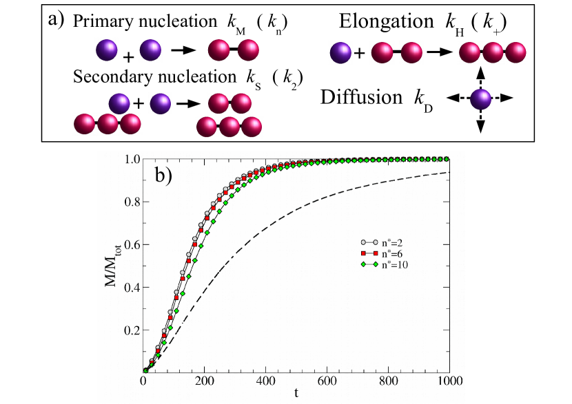
Figure 1: a) Schematic of the protein aggregation model describing the main processes involved: primary nucleation occurring with rate $k_{\rm M}$ (and correspondingly $k_{\rm n}$ in mean-field), polymer elongation with rate $k_{\rm H}$ ($k_{\rm+}$ in mean-field), secondary nucleation with rate $k_{\rm S}$ ($k_{\rm 2}$ in mean-field) and diffusion with rate $k_{\rm D}$ which is not described by mean-field theory. b) Simulations showing the dependence on the minimal polymer size $n^{*}$ needed to catalyze secondary nucleation of the aggregation curve, the polymer mass fraction $M/M_{\rm tot}$, obtained for $k_{\rm M}=4\cdot 10^{-4}$, $k_{D}=10^{-2}$, $k_{\rm S}=1$, $k_{\rm H}=10^{4}$ and $\rho=0.16$. The dashed line is the curve obtained in the limit $n^{*}\to\infty$, or equivalently in absence of secondary nucleation.

Simulations are performed using a variant of the protein aggregation model described in Ref. Budrikis et al. (2014) where individual protein molecules sit on a three dimensional cubic lattice. The model considers primary nucleation due to monomer-monomer interaction, polymer elongation due to addition of monomers to the polymer endpoints and secondary nucleation processes in which the rate of monomer-monomer interaction is enhanced when the process occurs close to a polymer (see Fig. 1a for an illustration) Cohen et al. (2011b). In particular, monomers diffuse with rate $k_{\rm D}$ and attach to neighboring monomers with rate $k_{\rm M}$ (primary nucleation) but when a monomer is nearest neighbor to a site containing a polymer composed of at least $n^{*}$ monomers, then the nucleation rate increases to $k_{\rm S}\gg k_{\rm M}$ (secondary nucleation). We do not consider polymer fragmentation, since this term is mostly relevant for samples under strong mechanical action Cohen et al. (2013), and some of the most important amyloid-forming proteins have been shown to exhibit aggregation kinetics dominated by secondary nucleation under quiescent conditions Cohen et al. (2013); Buell et al. (2014a). A monomer can attach to a polymer with rate $k_{\rm H}$ if it meets its endpoints. Polymers move collectively by reptation with a length-dependent rate $k_{\rm R}/i^{2}$, where $i$ is the number of monomers in the polymer (see Ref. Binder (1995) p. 89), and locally by end rotations, with rate $k_{\rm E}$, and kink moves with rate $k_{\rm K}$ (for a review of lattice polymer models see Binder (1995)). Simulations start with a constant number of $N$ monomers in a cubic system of size $L=m_{0}L_{0}$ (with $m_{0}$ an integer) where $L_{0}$ is the typical monomer diameter, with periodic boundary conditions in all directions. We perform numerical simulations using the Gillespie Monte Carlo algorithm Gillespie (1976) and measure time in units of $1/k_{\rm S}$ and rates in units of $k_{\rm S}$. We explore the behavior of the model by varying independently both the monomer concentration $\rho\equiv N/m_{0}^{3}$ and the number of monomers $N$ at fixed $\rho$, but also the rate constants. For the simulations results reported in the following, the rates describing polymer motion are chosen to be $k_{\rm E}=k_{\rm R}=k_{\rm K}=10^{-2}$ which is smaller or equal than the diffusion rate of the monomers $k_{\rm D}$.

As expected, secondary nucleation efficiently decreases the half-time before rapid polymerization. We illustrate this by changing the critical polymer size $n^{*}$ needed to induce secondary nucleation. We observe that the lower $n^{*}$ the shorter the half-time (see Fig. 1(b)). Currently, no experimental data exists on the value of $n^{*}$, but it can be expected to be of a similar magnitude as the smallest possible amyloid fibril, defined as the smallest structure for which monomer addition becomes independent of the size of the aggregate and an energetic downhill event.

Mean-field theory

The progress of reactions observed experimentally in bulk systems can be well approximated by a mean-field model Knowles et al. (2009); Cohen et al. (2011a, 2013), without fragmentation or depolymerization of polymers. Such models are in contrast to our three dimensional computational model, which describes also monomer diffusion and polymer motion due to reptation, kink motion and end-rotations, which are not treated by mean-field approximation. Despite this, it is still possible to fit polymerization curves resulting from three dimensional simulation results through mean-field theory with effective diffusion dependent parameters. The fact that both experimental and simulated polymerization curves are described by the same mean-field theory ensures that our model is appropriate to describe experiments. In the mean-field model, the evolution of the concentration $f_{j}$ of polymers of length $j\geq n_{c}$, where $n_{c}$ is the nucleation size, is given by Cohen et al. (2011a)

$$\dot{f}_{j}(t)=k_{n}m(t)^{n_{c}}\delta_{j,n_{c}}+2m(t)k_{+}f_{j-1}(t)-2m(t)k_{+}f_{j}(t)+k_{2}m(t)^{n_{2}}\sum_{i=n_{c}}^{\infty}if_{i}(t)\delta_{j,n_{2}},$$ (1)

where dots indicate time derivatives and $m(t)$ is the monomer concentration. The first term on the right-hand side represents an increase in the concentration of polymers of size $n_{c}$ due to polymer nucleation by aggregation of $n_{c}$ monomers with rate constant $k_{n}$; this is a generalized version of the dimer formation with rate constant $k_{\rm M}$ in the 3d model. The second term represents an increase in the concentration of polymers of size $j$ by attachment of a monomer to a polymer of size $j-1$, with rate constant $k_{+}$. The third term is the corresponding loss of concentration of polymers of size $j$ when they attach to a monomer. These two terms are the mean-field equivalent of the endpoint attachment of monomers to polymers with rate constant $k_{\rm H}$ in the 3d model. The final term represents secondary nucleation, which in the mean-field model is described as an increase in concentration of polymers of size $n_{2}$ (the secondary nucleus size) occurring at a rate proportional to the mass of polymers and with a rate constant $k_{2}$. By conservation of mass, the evolution of the monomer concentration is

$$\dot{m}(t)=-\sum_{i=n_{c}}^{\infty}i\dot{f}_{i}(t)$$ (2)

The evolution of the number concentration $P(t)=\sum_{j\geq n_{c}}f_{j}(t)$ and mass concentration $M(t)=\sum_{j\geq n_{c}}jf_{j}(t)$ can be found by summing over $j$ in (1). After some algebra, one obtains

$$\dot{P}(t)=k_{2}M(t)m(t)^{n_{2}}+k_{n}m(t)^{n_{c}},$$ (3)

$$\dot{M}(t)=2k_{+}m(t)P(t)+n_{2}k_{2}m(t)^{n_{2}}+n_{c}k_{n}m(t)^{n_{c}},$$ (4)

Analytical approximation Knowles et al. (2009); Cohen et al. (2011a, 2013) of the system of equations gives a solution that depends on two parameters, $\lambda=\sqrt{2k_{+}k_{n}m(0)^{n_{c}}}$ and $\kappa=\sqrt{2k_{+}k_{2}m(0)^{n_{2}+1}}$. We fit our data with the form given in Eq. 1 of Ref. Cohen et al. (2013), using a least squares method. Each curve is fitted independently. Diffusion plays an important role in the aggregation progress, shifting the aggregation curves as shown in Fig. 2a and Fig. 2b. For a considerable parameter range, however, the time evolution of the fractional polymer mass can be fitted by mean-field theory (lines in Fig. 2a and Fig. 2b) with effective parameters that now depend on the diffusion rate $k_{\rm D}$ (see Fig. 2c and 2d). Similarly, mean-field theory describes the density dependence of the aggregation curves as shown in Fig. 2b.

Fluctuations in protein aggregation

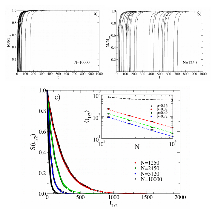
Figure 3: Half-time sample-to-sample fluctuations are due to extreme value statistics. Different replicates of the simulations display wide fluctuations in half-times especially for small numbers of monomers. a) Simulation results obtained for $N=10000$ monomers at $\rho=0.32$, $k_{\rm M}=4\cdot 10^{-6}$, $k_{\rm S}=1$, $k_{\rm H}=10^{4}$, $k_{\rm D}=10^{-2}$. The graph shows that the half-time $t_{1/2}$ is very close to the nucleation time $t_{0}$ at which the curves depart from zero. b) Same as panel a) but with $N=1250$. c) The complementary cumulative distributions of half-times obtained from simulations for different values of $N$ are in agreement with the theory described in the text. The inset shows that the average half-times for different concentrations $\rho$ as a function of $N$. The general trend is in agreement with experiments Knowles et al. (2011). Time is measured in units of $1/k_{\rm S}$.

Having confirmed that our computational model faithfully reproduces polymerization kinetics in macroscopic samples, we now turn to the main focus of the paper, the study of sample-to-sample fluctuations in small volumes, a feature that can not be studied with mean-field kinetics. When the sample volume is reduced, we observe increasing fluctuations in the aggregation kinetics as shown in Figs. 3a and 3b. These results are summarized in Fig 3c showing the complementary cumulative distributions of half-times for different monomer numbers $N$ and constant monomer concentration

$$S(t_{1/2})\equiv\int_{t_{1/2}}^{\infty}P(x)dx$$ (5)

where $P(x)$ is the probability density function and $t_{1/2}$ is defined as the half-time of the polymerization curve (i.e. the time at which $M/M_{0}=1/2$).

The steepness of the aggregation curves in Figs. 3a and 3b suggests that, for $k_{S}\gg k_{M}$, fluctuations are mostly ruled by the time of the first primary nucleation event, $t_{0}$, whose complementary cumulative distribution $S_{0}(t_{0})$ can be estimated analytically as

$$S_{0}(t_{0})=e^{-f_{M}k_{M}Nt_{0}}$$ (6)

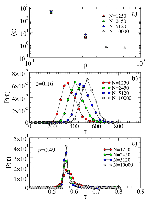
Figure 7: a) The mean delay time $\langle\tau\rangle$, obtained from numerical simulations, as a function of the number density $\rho$ for four different monomer numbers $N$. For any $N$ and $\rho$ the averages are calculated over the different numerical simulations outcomes. The distributions of delay times $\tau$ as a function of the number of monomers $N$ for b) $\rho=0.16$ and c) $\rho=0.49$. Here $k_{D}=10^{-2}$ and $k_{M}=4\cdot 10^{-6}$.

where $f_{M}$ is the average number of possible primary nucleation events per unit monomer. We estimate that $f_{M}=3\rho$ using a Poisson approximation, as we show in details in the following section. Note that Eq. 6 displays a size dependence that is reminiscent of extreme value statistics $S_{0}(x,N)=\exp(-NF(x))$ where $F(x)$ is a function that does not depend on $N$ Gumbel (2004); Weibull (1939). If $k_{S}\gg k_{M}$, the half-time $t_{1/2}$ differs from the nucleation time by a weakly fluctuating time $\tau$. This comes from the observation that, once the first primary nucleation event has happened, the polymerization follows rapidly, thanks to fast growth and secondary nucleation. This yields a weakly fluctuating delay $\tau(N,\rho)=t_{1/2}-t_{0}$, which in general depends on the number density $\rho$ and on the number of monomers $N$. The distribution and average values of $\tau$ are reported in Fig. 7. The average value of $\tau$ decreases with $\rho$ and displays only a smaller dependence on $N$. The distribution of $\tau$ is always peaked around its average but while at small values of $\rho$ the peak shifts with $N$ while the standard deviation remains constant, for higher values of $\rho$ only the standard deviation depends on $N$ and the peak position does not change. Since the fluctuations in $\tau$ are much smaller than the fluctuations of $t_{0}$ we can safely assume that $t_{1/2}\simeq t_{0}+\langle\tau\rangle$ for $t_{0}\geq 0$, so the complementary cumulative distribution takes the form

$$S(t_{1/2})=\left\{\begin{array}[]{ll}1&t_{1/2}\leq\langle\tau\rangle\\ S_{0}(t_{1/2}-\langle\tau\rangle)&t_{1/2}>\langle\tau\rangle.\end{array}\right.$$ (7)

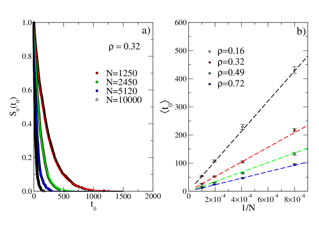
Figure 4: a) The complementary cumulative distribution functions $S(t_{0})$ for four different monomer numbers $N$ and density $\rho=0.32$. The symbols correspond to the numerical simulations while lines correspond to the theoretical predictions obtained from Eq. (6). b) The average time $\langle t_{0}\rangle$ as a function of $1/N$ for four different number densities. The theoretical predictions (dashed lines) are obtained from Eq.(13). Here $k_{D}=10^{-2}$ and $k_{M}=4\cdot 10^{-6}$

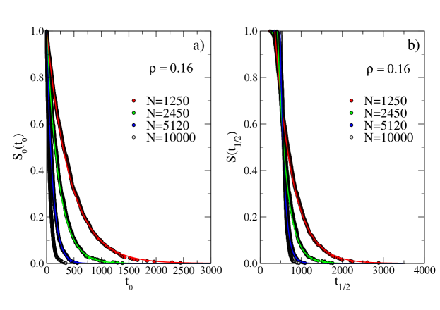
Figure 5: The complementary cumulative distribution functions $S(t_{0})$ (a) and $S(t_{1/2})$ (b) for four different monomer numbers $N$ and density $\rho=0.16$. The symbols correspond to the numerical simulations while the lines represent the theoretical predictions obtained from Eq. (6) and Eq. (7). Here $k_{D}=10^{-2}$ and $k_{M}=4\cdot 10^{-6}$.

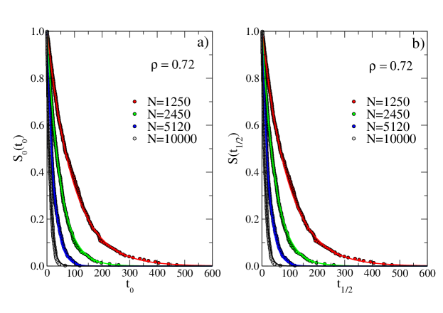
Figure 6: The complementary cumulative distribution functions $S(t_{0})$ (a) and $S(t_{1/2})$ (b) for four different monomer numbers $N$ and density $\rho=0.72$. The symbols correspond to the numerical simulations while he lines represent the theoretical predictions obtained from Eq.(6) and Eq.(7). Here $k_{D}=10^{-2}$ and $k_{M}=4\cdot 10^{-6}$.

The prediction of Eqs. 6 and 7 are in agreement with numerical simulations results for $S_{0}(t_{0})$ and $S(t_{1/2})$, respectively (see Figs. 3c and 4). In particular, the behavior of $S_{0}(t_{0})$ is obtained without any fitting parameters, while $S(t_{1/2})$ only needs the estimate of the single parameter $\langle\tau\rangle$ (additional comparisons for different values of $\rho$ are reported in Figs. 5 and 6). The corresponding average values of $\langle t_{1/2}\rangle$ are shown in the inset of Fig. 3c as a function of $N$ (see also Fig. 4b).

Theoretical derivation of the half-time distribution

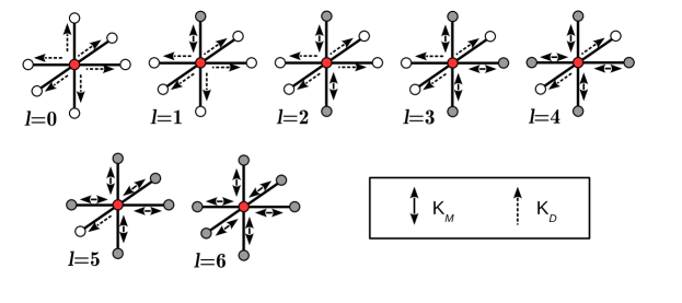
Figure 8: A schematic representation of the possibilities of diffusion (dashed arrow) and aggregation (double arrow) for a monomer (red circle) placed in the center of cubic lattice unit cell. The monomer partners for the dimerization (from $l=1$ to $l=6$) are colored in grey while the empty sites are represented by white circles. The aggregation and diffusion rate are, respectively, $k_{M}$ amd $k_{D}$.

In this section, we provide a detailed derivation of Eqs. 6 and 7 in the limit of relatively large diffusion when the system is well mixed. To this end, we consider a cubic lattice composed by $m_{0}^{3}$ nodes, in which $N$ monomers are placed randomly at time $t=0$. As illustrated in Fig. 8, each monomer $i$ sits near $l^{(i)}$ neighboring monomers and $6-l^{(i)}$ neighboring empty sites, where $l^{(i)}$ is in general a fluctuating time dependent quantity. In the model, each monomer $i$ can either diffuse into one of the $6-l^{(i)}$ empty sites or form a dimer with one of the $l^{(i)}$ neighboring monomers. Therefore, at any given time $t$ the number of possible diffusion events in the system is $n_{D}(t)=\sum_{i}(6-l^{(i)})$ and the number of possible aggregation events is $n_{M}(t)=1/2\sum_{i}l^{(i)}$, where the factor $1/2$ is needed to correct for the double counting of the number of monomer pairs. We can compute the time of first aggregation of $N$ monomers using Poisson statistics, considering for simplicity the case in which the number of possible aggregation events $n_{M}$ would not depend on time. In this case, the probability of having an aggregation event within $\Delta t$ is $n_{M}k_{M}\Delta t$. We can then divide the time interval $t_{0}$ in $n$ elementary time subintervals $\Delta t=\frac{t_{0}}{n}$, the rate of aggregation event at $t_{0}$, i.e. the probability per unit time to have the first dimer formed after a time interval $t_{0}$ has elapsed, is given by the following expression:

$$\tilde{P}_{0}(t_{0})=\lim_{n\to\infty}\left(1-n_{M}k_{M}\frac{t_{0}}{n}\right)^{n-1}n_{M}k_{M}=n_{M}k_{M}e^{-n_{M}k_{M}t_{0}}.$$ (8)

As stressed previously, $n_{M}$ and $n_{D}$ are in principle fluctuating quantities and therefore Eq.8 is not valid. Yet, as shown in Fig. 9: $n_{M}$ and $n_{D}$ are are both $i)$ stationary, $ii)$ ergodic, $iii)$ weakly fluctuating and $iv)$ linearly dependent on $N$, on average. Hence, the probability $\tilde{P}_{0}(t_{0})$ for a monomer to form a dimer at $t_{0}$ can reasonably be approximated by its ensemble average

$$P_{0}(t_{0})\simeq\langle\tilde{P}_{0}(t_{0})\rangle\simeq\langle n_{M}\rangle k_{M}e^{-f_{M}k_{M}Nt_{0}}$$ (9)

where we have replaced $n_{M}$ by its average value $\langle n_{M}\rangle$ and defined $f_{M}\equiv\frac{\langle n_{M}\rangle}{N}$. From Eq.(9), we easily obtain the complementary cumulative distribution function

$$S_{0}(t_{0})=\int_{t_{0}}^{\infty}d\tau P_{0}(\tau)=e^{-f_{M}k_{M}Nt_{0}},$$ (10)

recovering Eq. 6.

To conclude our calculation, we still need to evaluate $f_{M}$. To this end, we perform a discrete enumeration of the possible configurations of a single monomer, in the spirit of cluster expansions for percolation models. In particular, the six relevant configurations for a single monomer in contact with other monomers are reported in Fig. 8. The weight $p_{l}$ of a configuration in which a monomer has $l$ occupied neighbors is assumed to be given by the binomial distribution

$$p_{l}=\frac{6!}{l!(6-l)!}\rho^{l}(1-\rho)^{6-l}.$$ (11)

This single particle picture suggests that the average number of primary nucleation events per monomer $f_{M}$, corresponds to the average number of nearest neighbors $\langle l\rangle$, divided by a factor 2 since any nucleation event encompasses 2 particles. With a similar reasoning, we estimate $f_{D}=6-\langle l\rangle$, i.e. the average number of empty directions. Then, from the binomial distribution (11) we get $f_{M}=\frac{6\rho}{2}$ and $f_{D}=6(1-\rho)$. Using these values in Eq. 6 and Eq.(7), we obtain agreement with numerical simulations as illustrated in Figs. 5 and 6 (panels (a) and (b) respectively) for different values of $\rho$.

Finally, we calculate the averages of the first aggregation time and the half-time as $\langle t_{0}\rangle=\int_{0}^{\infty}dt_{0}\,t_{0}P_{0}(t_{0})$ and $\langle t_{1/2}\rangle=\int_{0}^{\infty}dt_{1/2}\,t_{1/2}P(t_{1/2})$, where $P(t_{1/2})=-\frac{dS(t_{1/2})}{dt_{1/2}}$. The expression for $\langle t_{0}\rangle$ is given by

$$\langle t_{0}\rangle=\frac{1}{3\rho k_{M}N}.$$ (12)

In Fig. 4b we show the perfect agreement of the theoretical estimate given by Eq.(12) with the numerical values of the average time for the first primary nucleation event as a function of $1/N$, for several densities. Notice that no fitting parameters are involved. The average time of $t_{1/2}$ follows from $\langle t_{1/2}\rangle=\langle t_{0}\rangle+\langle\tau\rangle$: the inset of Fig. 3c confirms the agreement between the theoretical estimates (dashed lines) and the numerical values (symbols).

Statistical analysis of seed detection tests

While the fluctuations we observe are intrinsic to the random nature of nucleation events, the ones usually encountered in bulk experiments are likely due to contamination or differences in initial conditions Giehm and Otzen (2010); Uversky et al. (2001); Grey et al. (2015). In those bulk systems ($\mu$l and larger), the number of protein molecules involved in the aggregation process is extremely large, even at low concentrations, so that we can exclude intrinsic kinetic fluctuations. For instance, a volume of 100$\mu$l at a concentration of 1$\mu$M still contains $10^{14}$ monomers, leading to a large number (hundreds to thousands) of nucleation events per second for a realistic value of the nucleation rate Cohen et al. (2013); Buell et al. (2014b). However, if the relevant volumes are made small enough (pico- to nanolitres), the stochastic nature of primary nucleation can be directly observed. This has been exploited by aggregation experiments performed inside single microdroplets, where individual nucleation events could be observed, due to their amplification by secondary processes Knowles et al. (2011). In these experiments, the average half-time is found to scale with volume in a similar manner to what is shown in the inset of Fig. 3, thus in agreement with our simulations.

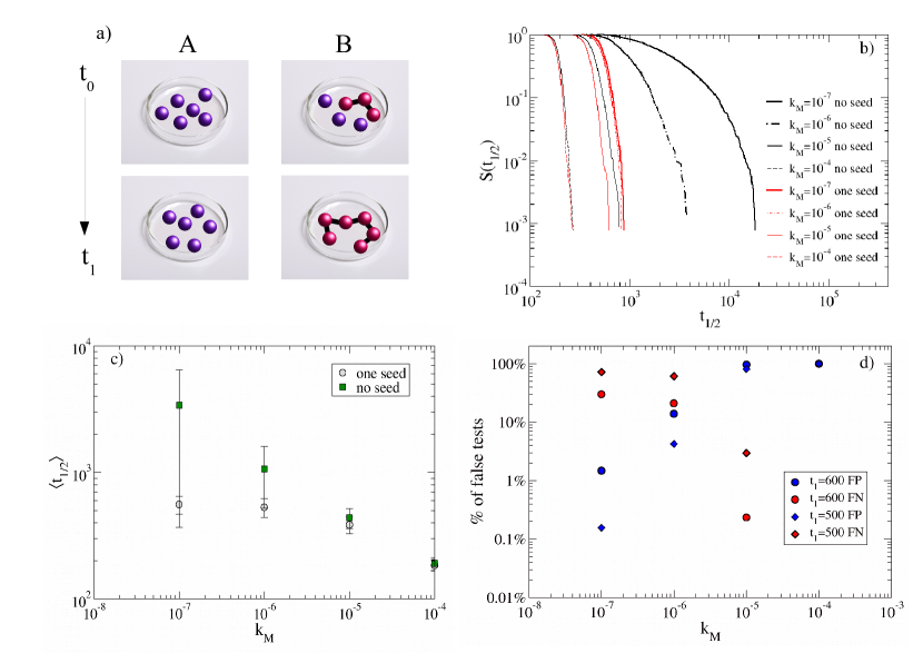
Figure 10: Intrinsic fluctuations rule errors in the detection of protein aggregation prone samples. a) A test to detect seeds for protein aggregation is based on small volume sampling of protein solutions at time $t_{0}=0$ and on the assumption that only seeded samples (e. g. sample B) would form aggregate at time $t_{1}$. b) Simulations allow to compute the distribution of half-times for samples with and without a seed as a function of the rate of primary nucleation $k_{M}$. Data are obtained sampling over $n=1200$ independent realization. c) Average half-time ($\pm$ standard deviation) as a function of the rate of primary nucleation $k_{M}$. d) Fraction of false positives (FP) and false negatives (FN) for testing times $t_{1}=600$ and $t_{1}=500$. Time is measured in units of $1/k_{\rm S}$, $N=1250$.

We are now in a position to use our model to design a test in silico to detect the presence of pre-formed polymers, that act as seeds and nucleation sites for the secondary nucleation process, and that are thus amplified. As illustrated in Fig. 10a, the test considers a set of small volume samples containing protein solutions with a given concentration at time $t_{0}=0$. The aim of the test is to detect the samples containing at least one seed (case B in Fig. 10a). In an ideal experiment, the size of the microdroplets would be adjusted such that most droplets contain no seeds, some contain one seed, and the proportion of droplets containing more than one seed is negligible. In practice, these conditions can be easily adjusted experimentally by progressively reducing droplet volumes until only a small fraction of them display aggregates. After a fixed time $t_{1}\sim\langle\tau\rangle$, one can observe which samples contain macroscopic, detectable amounts of aggregates, enabling exact quantification of the number of aggregates present in the initial sample. Ideally the test should be positive only when at least one seed was initially present, but given the large fluctuations intrinsic to the nucleation processes we demonstrated above, as well as the competition with de novo nucleation, there is a chance for false tests. In particular, a false positive test occurs when an unseeded sample is found to contain aggregates, while a false negative test corresponds to the case in which a seeded sample does not produce detectable amounts of aggregates within the time scale of the experiment.

In Fig. 10b we report the complementary cumulative distribution of aggregation half-times $t_{1/2}$ as a function of the primary nucleation rate $k_{\rm M}$ for samples with or without seeds, in this case a single pre-formed trimer. For small values of $k_{\rm M}$, seeded and unseeded samples yield distinct results, as also illustrated by the average half-times reported in Fig. 10c. As the value of $k_{\rm M}$ increases, however, the distributions become closer in the two cases. In Fig. 10d, we quantify the fraction of false positive and false negative tests for two different testing times (e.g. $t_{1}=500$ and $t_{1}=600$). As expected, for large $k_{\rm M}$ errors are very likely and the test would not be reliable. For intermediate values of $k_{\rm M}$, one can try to adjust $t_{1}$ to reduce possible errors with a caveat: decreasing $t_{1}$ reduces false positive errors, but at the same time increases false negatives (Fig. 10d). It is, however, possible to optimize $t_{1}$ so that both types of errors are minimized. In an experimental realisation of such a setup, the most important system parameter that needs to be optimized for any given protein is the ratio of secondary nucleation rate to primary nucleation rate. Due to potentially different dependencies of these two rates on the monomer concentration Meisl et al. (2014), pH Buell et al. (2014a) and potentially other factors, such as temperature, salt concentration etc., it is possible to fine tune this ratio and adjust it to a value that allows for an easy discrimination between droplets that do contain a seed aggregate and those that do not.

Conclusions

In conclusion, we study protein polymerization in a three dimensional computational model and elucidate the role of protein diffusion in the polymerization process. Most theoretical studies of protein aggregation neglect completely the role of diffusion and any other spatial effect. When the polymer diffusion and elongation rates are large enough we recover the standard polymerization curves that can also be obtained from mean-field analytical treatments and that can be used to fit, for example, kinetic data of amyloid $\beta$ aggregation Cohen et al. (2013). It would be interesting to explore if for small diffusion rates and small densities mean-field kinetics would eventually fail to describe the results, but this is a challenging computational task. At low densities, diffusion could play an important since a critical timescale would be set by the time needed by two monomers to meet before aggregating. This time-scale can be estimated considering the time for a monomer to cover a distance $x_{D}\sim\rho^{-1/3}$, yielding $t_{D}\sim x_{D}^{2}/D\sim D^{-1}\rho^{-2/3}$. This timescale is not relevant for our simulations since at the relatively high densities we study a considerable fraction of monomers are close to at least another monomer (see $n_{M}$ in Fig. 9a). Consequently, the distribution of the first aggregation time does not depend on the diffusion rate $k_{D}$ (see Eq. 6). The half-time distribution, however, depends on diffusion even in this regime (Fig. 2).

Our simulations show intrinsic sample-to-sample fluctuations that become very large in the limit of small volumes and low aggregation rates. We show that the corresponding half-time distributions are described by Poisson statistics and display size dependence. As a consequence of this, the average half-times scale as the inverse of the sample volume, in agreement with insulin aggregation experiments performed in microdroplets Knowles et al. (2011) and with calculations based on a master-equation approach Szavits-Nossan et al. (2014). We use this result to design and validate in silico a pre-clinical screening test based on a subdivision of the macroscopic sample volume that will ultimately allow the determination of the exact number of aggregates that was initially present. This is the first step to develop microarray-based in vitro tests for early diagnosis of neurodegenerative diseases.

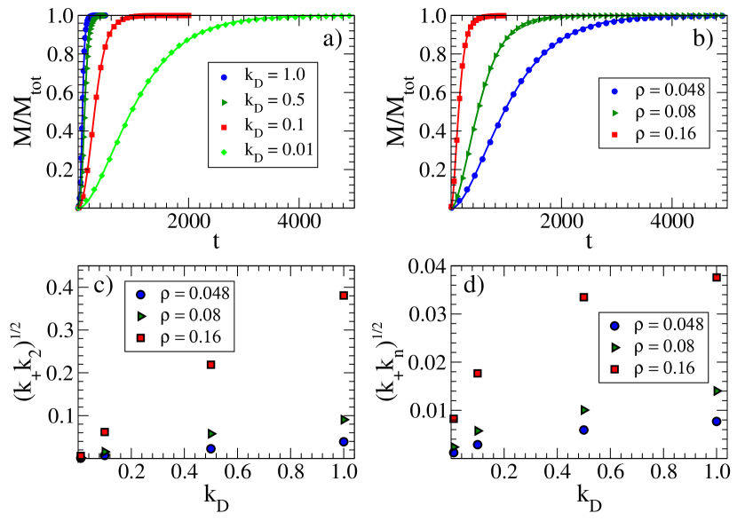
Figure 2: Protein aggregation depends on monomer diffusion: a) Simulations showing the diffusion dependence of the aggregation curve, the polymer mass fraction $M/M_{\rm tot}$, obtained for $k_{\rm M}=4\cdot 10^{-4}$, $k_{\rm S}=k_{\rm H}=1$, $N=2450$ and $\rho=0.048$. The curves are well fit by mean-field theory (full lines) with effective parameters that depend on $k_{\rm D}$. b) Simulations of the density dependence of the polymer mass fraction for $N=2450$, $k_{\rm M}=4\cdot 10^{-4}$, $k_{\rm H}=1$ and $k_{\rm D}=10^{-2}$. Fits by mean-field theory are plotted as lines with effective parameters reported in the panels c) and d). Time is measured in units of $1/k_{\rm S}$. c)-d):The effective mean-field parameters $\sqrt{k_{+}k_{2}}$ and $\sqrt{k_{+}k_{n}}$ obtained by fitting simulations performed for $k_{\rm M}=4\cdot 10^{-4}$, $k_{\rm S}=k_{\rm H}=1$ as a function of the concentration $\rho$ and the diffusion rate $k_{\rm D}$.

Figure 9: a) The number of possible primary nucleation and diffusion events ($n_{M}$ and $n_{D}$, respectively) are a linear function of the number of monomers $N$. b) The corresponding frequencies $f_{M}$ and $f_{D}$ fluctuate very little in time. Here $k_{D}=10^{-2}$, $k_{M}=4\cdot 10^{-6}$, $N=2450$ and $\rho=0.16$.

References

- Jarrett and Lansbury (1993) Joseph T Jarrett and Peter T Lansbury, “Seeding “one-dimensional crystallization” of amyloid: A pathogenic mechanism in Alzheimer’s disease and scrapie?” Cell 73, 1055–1058 (1993).
- Buell et al. (2014a) Alexander K Buell, Céline Galvagnion, Ricardo Gaspar, Emma Sparr, Michele Vendruscolo, Tuomas P J Knowles, Sara Linse, and Christopher M Dobson, “Solution conditions determine the relative importance of nucleation and growth processes in -synuclein aggregation,” Proc Natl Acad Sci U S A 111, 7671–6 (2014a).
- Grey et al. (2015) Marie Grey, Christopher J Dunning, Ricardo Gaspar, Carl Grey, Patrik Brundin, Emma Sparr, and Sara Linse, “Acceleration of -synuclein aggregation by exosomes,” J Biol Chem 290, 2969–82 (2015).
- Galvagnion et al. (2015) Céline Galvagnion, Alexander K Buell, Georg Meisl, Thomas C T Michaels, Michele Vendruscolo, Tuomas P J Knowles, and Christopher M Dobson, “Lipid vesicles trigger -synuclein aggregation by stimulating primary nucleation,” Nat Chem Biol 11, 229–34 (2015).
- Vacha et al. (2014) Robert Vacha, Sara Linse, and Mikael Lund, “Surface effects on aggregation kinetics of amyloidogenic peptides,” J Am Chem Soc 136, 11776–82 (2014).
- Ruschak and Miranker (2007) Amy M Ruschak and Andrew D Miranker, “Fiber-dependent amyloid formation as catalysis of an existing reaction pathway.” Proc Natl Acad Sci U S A 104, 12341–12346 (2007).
- Cohen et al. (2013) Samuel I. A. Cohen, Sara Linse, Leila M. Luheshi, Erik Hellstrand, Duncan A. White, Luke Rajah, Daniel E. Otzen, Michele Vendruscolo, Christopher M. Dobson, and Tuomas P. J. Knowles, “Proliferation of amyloid-42 aggregates occurs through a secondary nucleation mechanism,” Proceedings of the National Academy of Sciences 110, 9758 (2013).
- Peelaerts et al. (2015) W. Peelaerts, L. Bousset, A. Van der Perren, A. Moskalyuk, R. Pulizzi, M. Giugliano, C. Van den Haute, R. Melki, and V. Baekelandt, “-synuclein strains cause distinct synucleinopathies after local and systemic administration.” Nature 522, 340–344 (2015).
- Morales et al. (2012) Rodrigo Morales, Claudia Duran-Aniotz, Rodrigo Diaz-Espinoza, Manuel V Camacho, and Claudio Soto, “Protein misfolding cyclic amplification of infectious prions.” Nat Protoc 7, 1397–1409 (2012).
- Salvadores et al. (2014) Natalia Salvadores, Mohammad Shahnawaz, Elio Scarpini, Fabrizio Tagliavini, and Claudio Soto, “Detection of misfolded a? oligomers for sensitive biochemical diagnosis of alzheimer’s disease.” Cell Rep 7, 261–268 (2014).
- Arosio et al. (2014) Paolo Arosio, Risto Cukalevski, Birgitta Frohm, Tuomas P J Knowles, and Sara Linse, “Quantification of the concentration of a42 propagons during the lag phase by an amyloid chain reaction assay.” J Am Chem Soc 136, 219–225 (2014).
- Theberge et al. (2010) Ashleigh B Theberge, Fabienne Courtois, Yolanda Schaerli, Martin Fischlechner, Chris Abell, Florian Hollfelder, and Wilhelm T S Huck, “Microdroplets in microfluidics: an evolving platform for discoveries in chemistry and biology.” Angew Chem Int Ed Engl 49, 5846–5868 (2010).
- Knowles et al. (2011) Tuomas P J Knowles, Duncan A White, Adam R Abate, Jeremy J Agresti, Samuel I A Cohen, Ralph A Sperling, Erwin J De Genst, Christopher M Dobson, and David A Weitz, “Observation of spatial propagation of amyloid assembly from single nuclei,” Proc Natl Acad Sci U S A 108, 14746–51 (2011).
- Knowles et al. (2009) Tuomas P J Knowles, Christopher A Waudby, Glyn L Devlin, Samuel I A Cohen, Adriano Aguzzi, Michele Vendruscolo, Eugene M Terentjev, Mark E Welland, and Christopher M Dobson, “An analytical solution to the kinetics of breakable filament assembly.” Science 326, 1533–1537 (2009).
- Cohen et al. (2011a) Samuel I. A. Cohen, Michele Vendruscolo, Christopher M. Dobson, and Tuomas P. J. Knowles, “Nucleated polymerization with secondary pathways. ii. determination of self-consistent solutions to growth processes described by non-linear master equations,” The Journal of Chemical Physics 135, 065106 (2011a).
- Szavits-Nossan et al. (2014) Juraj Szavits-Nossan, Kym Eden, Ryan J Morris, Cait E MacPhee, Martin R Evans, and Rosalind J Allen, “Inherent variability in the kinetics of autocatalytic protein self-assembly,” Phys Rev Lett 113, 098101 (2014).
- Budrikis et al. (2014) Zoe Budrikis, Giulio Costantini, Caterina A M La Porta, and Stefano Zapperi, “Protein accumulation in the endoplasmic reticulum as a non-equilibrium phase transition,” Nat Commun 5, 3620 (2014).
- Buell et al. (2012) Alexander K Buell, Anne Dhulesia, Duncan A White, Tuomas P J Knowles, Christopher M Dobson, and Mark E Welland, “Detailed analysis of the energy barriers for amyloid fibril growth,” Angew Chem Int Ed Engl 51, 5247–51 (2012).
- Cohen et al. (2011b) Samuel I A Cohen, Michele Vendruscolo, Mark E Welland, Christopher M Dobson, Eugene M Terentjev, and Tuomas P J Knowles, “Nucleated polymerization with secondary pathways. I. time evolution of the principal moments.” J Chem Phys 135, 065105 (2011b).
- Binder (1995) K. Binder, ed., Monte Carlo and Molecular Dynamics Simulations in Polymer Science (Oxford University Press, New York, Oxford, 1995).
- Gillespie (1976) Daniel T Gillespie, “A general method for numerically simulating the stochastic time evolution of coupled chemical reactions,” Journal of Computational Physics 22, 403 – 434 (1976).
- Gumbel (2004) E. J. Gumbel, Statistics of Extremes (Columbia University Press, New York, 2004).
- Weibull (1939) W. Weibull, A statistical theory of the strength of materials, edited by Generalstabens litografiska anstalts foerlag (Stockholm, 1939).
- Giehm and Otzen (2010) Lise Giehm and Daniel E Otzen, “Strategies to increase the reproducibility of protein fibrillization in plate reader assays,” Anal Biochem 400, 270–81 (2010).
- Uversky et al. (2001) V N Uversky, J Li, and A L Fink, “Evidence for a partially folded intermediate in alpha-synuclein fibril formation,” J Biol Chem 276, 10737–44 (2001).
- Buell et al. (2014b) Alexander K Buell, Christopher M Dobson, and Tuomas P J Knowles, “The physical chemistry of the amyloid phenomenon: thermodynamics and kinetics of filamentous protein aggregation.” Essays Biochem 56, 11–39 (2014b).
- Meisl et al. (2014) Georg Meisl, Xiaoting Yang, Erik Hellstrand, Birgitta Frohm, Julius B Kirkegaard, Samuel I A Cohen, Christopher M Dobson, Sara Linse, and Tuomas P J Knowles, “Differences in nucleation behavior underlie the contrasting aggregation kinetics of the a40 and a42 peptides,” Proc Natl Acad Sci U S A 111, 9384–9 (2014).