On the joint distribution of first-passage time and first-passage area of drifted Brownian motion

Abstract

For drifted Brownian motion $X(t)=x-\mu t+B_{t}\ (\mu>0)$ starting from $x>0,$ we study the joint distribution of the first-passage time below zero, $\tau(x),$ and the first-passage area, $A(x),$ swept out by $X$ till the time $\tau(x).$ In particular, we establish differential equations with boundary conditions for the joint moments $E[\tau(x)^{m}A(x)^{n}],$ and we present an algorithm to find recursively them, for any $m$ and $n.$ Finally, the expected value of the time average of $X$ till the time $\tau(x)$ is obtained.

Keywords: First-passage time, first-passage area, one-dimensional diffusion.
Mathematics Subject Classification: 60J60, 60H05, 60H10.

1 Introduction

This a continuation of the article [1], where we have studied the probability distribution of the first-passage area (FPA) $A(x),$ swept out by a one-dimensional jump-diffusion process $X(t),$ starting from $x>0,$ till its first-passage time (FPT) $\tau(x)$ below zero. In particular, in [1] it was shown that the Laplace transform and the moments of $A(x)$ are solutions to certain partial differential-difference equations with outer conditions.

In the present paper, we aim to study the joint distribution of $\tau(x)$ and $A(x),$ in the special case when $X(t)$ is Brownian motion with negative drift $-\mu,$ that is, $X(t)=x-\mu t+B_{t},$ where $B_{t}$ denotes standard Brownian motion. We state differential equations for the Laplace transform of the two-dimensional random variable $(\tau(x),A(x)),$ and for the joint moments $E[\tau(x)^{m}A(x)^{n}]$ of the FPT and FPA; moreover, we present an algorithm to find them recursively, for any $m$ and $n.$ In particular, closed formulae for $E[\tau(x)A(x)]$ and the correlation between $\tau(x)$ and $A(x),$ are explicitly obtained; they match existing results, obtained in [7] in terms of the Airy function $Ai(z)$ by using its asymptotic expansion as $z\rightarrow\infty.$ Furthermore, we find the expected value of the time average of $X(t)$ till its FPT below zero.

The difference compared to similar articles (see e.g. [7]) is that the results of the present paper are obtained without the use of special functions.

Over the years, several authors have dealt with first-passage area for Brownian motion with negative drift (see [5], [7], [8], [9], [10], [11] and references in [1]); the FPA has interesting applications, for instance, in Queueing Theory, if one identifies $X(t)$ with the length of a queue at time $t,$ and $\tau(x)$ with the busy period, that is the time until the queue is first empty; then, $A(x)$ represents the cumulative waiting time experienced by all the “customers” during a busy period. The FPA arises also in solar physics studies, non-oriented animal movement patterns, and DNA breathing dynamics (see references in [7]). For other examples from Economics and Biology, see [1].

The paper is organized as follows. Section 2 contains the main results: in subsection 2.1 we deal with the Laplace transform of $(\tau(x),A(x))$ and the joint moments of $A(x)$ and $\tau(x),$ precisely, in 2.1.1 we find explicitly $E[\tau(x)A(x)],$ and in 2.1.2 we establish ODEs for the joint moments $E[\tau(x)^{m}A(x)^{n}]$ of order $n+m,\ n,m\geq 0;$ moreover we present an algorithm to find recursively $E[\tau(x)^{m}A(x)^{n}],$ for any $m$ and $n;$ subsection 2.2 is devoted to find the expected value of the time average of $X(t)$ till its FPT below zero. Section 3 contains conclusions and final remarks.

2 Notations, formulation of the problem and main results

For $x>0$ and $\mu>0,$ we consider Brownian motion with negative drift $-\mu,$ that is $X(t)=x-\mu t+B_{t},$ where $B_{t}$ is standard Brownian motion. We denote by

$$\tau(x)=\tau^{\mu}(x)=\inf\{t>0:X(t)\leq 0|X(0)=x\}$$ (2.1)

the FPT below zero of $X(t);$ since the drift $-\mu$ is negative, $\tau(x)$ is finite with probability one. Let $U$ be a functional of the process $X,$ and for $\lambda>0$ denote by

$$M_{U,\lambda}(x)=E\left[e^{-\lambda\int_{0}^{\tau(x)}U(X(s))ds}\right]$$ (2.2)

the Laplace transform of the integral $\int_{0}^{\tau(x)}U(X(s))ds.$ We recall from [1] the following:

Theorem 2.1

For $\lambda>0,\ M_{U,\lambda}(x)=E\left[e^{-\lambda\int_{0}^{\tau(x)}U(X(s))ds}\right]$ is the solution of the problem with boundary conditions ($M^{\prime}$ and $M^{\prime\prime}$ denote first and second derivative with respect to $x)$ :

$$\begin{cases}\frac{1}{2}M^{\prime\prime}_{U,\lambda}(x)-\mu M^{\prime}_{U,\lambda}(x)=\lambda U(x)M_{U,\lambda}(x)\\ M_{U,\lambda}(0)=1\\ \lim_{x\rightarrow+\infty}M_{U,\lambda}(x)=0\ .\end{cases}$$ (2.3)

Moreover, the n-th order moments $T_{n}(x)$ of $\int_{0}^{\tau(x)}U(X(s))ds,$ if they exist finite, satisfy the recursive ODEs:

$$\frac{1}{2}T^{\prime\prime}_{n}(x)-\mu T^{\prime}_{n}(x)=-nU(x)T_{n-1}(x),\ {\rm for}\ x>0$$ (2.4)

with the condition $T_{n}(0)=0,$ plus an appropriate additional condition.

$\Box$

(i) The moment generating function of $\tau^{\mu}(x)$

By solving (2.3) with $U(x)=1,$ one explicitly obtains:

$$M_{U,\lambda}(x)=E(\exp(-\lambda\tau^{\mu}(x))=\exp[-x(\sqrt{\mu^{2}+2\lambda}-\mu)].$$ (2.5)

This Laplace transform can be explicitly inverted (see [6]), so obtaining the well-known expression of the density of $\tau^{\mu}(x):$

$$f_{\tau^{\mu}(x)}(t)=\frac{x}{\sqrt{2\pi}t^{3/2}}e^{-(x-\mu t)^{2}/2t},$$ (2.6)

that is the inverse Gaussian density. For $\mu>0$ the moments $T_{n}(x)=E(\tau^{\mu}(x))^{n}$ of any order $n,$ are finite and they can be easily obtained by calculating $(-1)^{n}[\partial^{n}M_{U,\lambda}(x)/\partial\lambda^{n}]_{\lambda=0}.$ We obtain, for instance, $E(\tau^{\mu}(x))=\frac{x}{\mu}$ and $E((\tau^{\mu}(x))^{2})=\frac{x}{\mu^{3}}+\frac{x^{2}}{\mu^{2}}.$ Note that $E(\tau^{\mu}(x))\rightarrow+\infty,$ as $\mu\rightarrow 0.$ As easily seen, for any $x>0,$ it results $M_{U,\lambda}(x)\rightarrow 1,$ as $\mu\rightarrow+\infty,$ or, equivalently, $\tau^{\mu}(x)$ converges to $0$ in distribution, and so $E((\tau^{\mu}(x))^{n})\rightarrow 0,$ as $\mu\rightarrow+\infty,$ for any $n$ and $x>0.$

(ii) The moments of $A^{\mu}(x)=\int_{0}^{\tau^{\mu}(x)}(x-\mu t+B_{t})dt.$

For $U(x)=x$ the equation of problem (2.3) becomes

$$\frac{1}{2}M^{\prime\prime}_{U,\lambda}-\mu M^{\prime}_{U,\lambda}=\lambda xM_{U,\lambda},$$ (2.7)

where now $M_{U,\lambda}(x)=E(e^{-\lambda A^{\mu}(x)}).$ It is the Schrodinger equation for a quantum particle moving in a uniform field (see e.g [8], [9]). Its explicit solution cannot be found in terms of elementary functions, however it can be written in terms of the Airy function (see [3], [8]) though, for $\mu\neq 0,$ it is impossible to invert the Laplace transform $M_{U,\lambda}$ to obtain the probability density of $A^{\mu}(x).$

In the special case $\mu=0,$ it can be shown ([8]) that the solution of (2.7) is:

$$M_{U,\lambda}(x)=3^{2/3}\Gamma\left(\frac{2}{3}\right){\rm Ai}(2^{1/3}\lambda^{1/3}x),$$ (2.8)

where ${\rm Ai}(z)$ denotes the standard Airy function, which obeys the ODE ${\rm Ai}^{\prime\prime}(z)=z{\rm Ai}(z)$ (see [3]); then, by inverting this Laplace transform one finds that the first-passage area density is ([8]):

$$f_{A^{0}(x)}(a)=\frac{2^{1/3}}{3^{2/3}\Gamma(\frac{1}{3})}\ \frac{x}{a^{4/3}}\ e^{-2x^{3}/9a}\ .$$ (2.9)

Thus, the distribution of $A^{0}(x)$ has an algebraic tail of order $\frac{4}{3}$ and so the moments of all orders are infinite.

For $\mu>0,$ closed form expression for the first two moments of $A^{\mu}(x)$ have been obtained in [1], by solving (2.4) with $U(x)=x,$ with appropriate conditions. The mean first-passage area is

$$E(A^{\mu}(x))=\frac{x^{2}}{2\mu}+\frac{x}{2\mu^{2}}\ ,$$ (2.10)

while the second moment of $A^{\mu}(x)$ is

$$E[(A^{\mu}(x))^{2}]=\frac{x^{4}}{4\mu^{2}}+\frac{5x^{3}}{6\mu^{3}}+\frac{5x^{2}}{4\mu^{4}}+\frac{5x}{4\mu^{5}}\ .$$ (2.11)

Finally, by (2.10) and (2.11), the variance of $A^{\mu}(x)$ is obtained:

$$Var(A^{\mu}(x))=E(A^{\mu}(x)^{2})-E^{2}(A^{\mu}(x))=\frac{x^{3}}{3\mu^{3}}+\frac{x^{2}}{\mu^{4}}+\frac{5x}{4\mu^{5}}\ .$$ (2.12)

Since a closed form expression of the density of the first-passage area $A^{\mu}(x)$ cannot be found for $\mu>0,$ it must be studied numerically; indeed, it was estimated in [1] by simulating a large number of trajectories of Brownian motion with drift $-\mu,$ starting from the initial state $x>0.$ For completeness, we report Figure 1 from [1], which shows the shape of the estimated FPA density for $x=1,$ as a function of $\mu>0.$

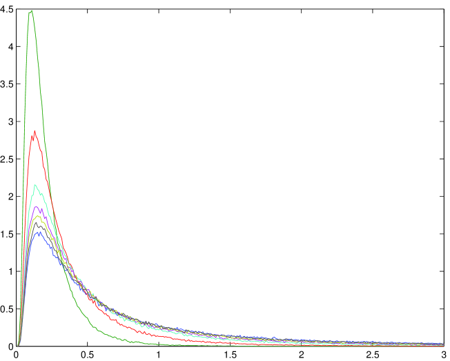
Figure 1: Estimated density of the first-passage area $A^{\mu}(x)$ for $x=1$ and several values of $\mu.$ From top to bottom, with respect to the peak of the curve: $\mu=3;\ \mu=2;\ \mu=1.5;\ \mu=1.3;\ \mu=1.2;\ \mu=1.1;\ \mu=1.$

2.1 Joint moments of $A(x)$ and $\tau(x).$

Now, we go to study the joint distribution of $A(x)$ and $\tau(x);$ our aim is to find an explicit form for the joint moments of $A(x)$ and $\tau(x).$ For $\lambda=(\lambda_{1},\lambda_{2})\in\mathbb{R}_{+}^{2},$ the joint Laplace transform of $(A(x),\tau(x))$ is

$$M_{\lambda}(x)=M_{(\lambda_{1},\lambda_{2})}(x)=E\left(e^{-\lambda_{1}\tau(x)-\lambda_{2}A(x)}\right)$$

$$=E\left(e^{-\lambda_{1}\tau(x)-\lambda_{2}\int_{0}^{\tau(x)}X(t)dt}\right)=E\left(e^{-\int_{0}^{\tau(x)}(\lambda_{1}+\lambda_{2}X(t))dt}\right).$$ (2.13)

By using (2.3) with $\lambda=1$ and $U(x)=\lambda_{1}+\lambda_{2}x,$ we obtain that the function $M_{(\lambda_{1},\lambda_{2})}(x)$ solves the problem:

$$\begin{cases}\frac{1}{2}\frac{d^{2}}{dx^{2}}M_{\lambda}(x)-\mu\frac{d}{dx}M_{\lambda}(x)=(\lambda_{1}+\lambda_{2}x)M_{\lambda}(x),\\ M_{\lambda}(0)=1,\\ \lim_{x\rightarrow+\infty}M_{\lambda}(x)=0.\end{cases}$$ (2.14)

Explicitly one has (see [7]):

$$M_{\lambda}(x)=e^{\mu x}\left[Ai\left(\frac{\mu^{2}+2\lambda_{1}+2\lambda_{2}x}{2^{2/3}\lambda_{2}^{2/3}}\right)\right]/\left[Ai\left(\frac{\mu^{2}+2\lambda_{1}}{2^{2/3}\lambda_{2}^{2/3}}\right)\right],$$ (2.15)

where ${\rm Ai}(z)$ is the standard Airy function. The joint moments $E[\tau^{m}(x)A^{n}(x)],$ if they exist finite, can be obtained by taking the partial derivative of order $m+n$ at $\lambda=0,$ i.e.

$$E\left[\tau^{m}(x)A^{n}(x)\right]=(-1)^{m+n}\frac{\partial^{m}}{\partial\lambda_{1}^{m}}\frac{\partial^{n}}{\partial\lambda_{2}^{n}}M_{\lambda}(x)\Big{|}_{\lambda_{1}=\lambda_{2}=0},$$

however these calculations involve special functions. To avoid this, we use the problem (2.14) to write down ODEs for $E[\tau^{m}(x)A^{n}(x)];$ in the next subsection, we start with $m=n=1.$

2.1.1 Correlation between $A(x)$ and $\tau(x)$

We have:

$$\frac{\partial}{\partial\lambda_{1}}M_{\lambda}(x)\Big{|}_{\lambda_{1}=\lambda_{2}=0}=-E(\tau(x)),\ \frac{\partial}{\partial\lambda_{2}}M_{\lambda}(x)\Big{|}_{\lambda_{1}=\lambda_{2}=0}=-E(A(x)),$$

$$\frac{\partial^{2}}{\partial\lambda_{1}\partial\lambda_{2}}M_{\lambda}(x)\Big{|}_{\lambda_{1}=\lambda_{2}=0}=E(\tau(x)A(x)),$$

and:

$$\frac{\partial^{2}}{\partial\lambda_{1}\partial\lambda_{2}}[(\lambda_{1}+\lambda_{2}x)M_{\lambda}(x)]\Big{|}_{\lambda_{1}=\lambda_{2}=0}=-xE(\tau(x))-E(A(x)).$$

Therefore, by applying $\partial^{2}/\partial\lambda_{1}\partial\lambda_{2}$ to both members of (2.14), calculating for $\lambda_{1}=\lambda_{2}=0,$ we obtain:

$$\frac{1}{2}\frac{d^{2}}{dx^{2}}E[\tau(x)A(x)]-\mu\frac{d}{dx}E[\tau(x)A(x)]=-xE(\tau(x))-E(A(x)).$$

Thus, recalling that $E(\tau(x))=x/\mu,\ E(A(x))=x/2\mu^{2}+x^{2}/\ 2\mu,$ we get:

Theorem 2.2

$V(x):=E[\tau(x))A(x)]$ is the solution of the problem:

$$\begin{cases}\frac{1}{2}V^{\prime\prime}(x)-\mu V^{\prime}(x)=-\frac{3x^{2}}{2\mu}-\frac{x}{2\mu^{2}},\\ V(0)=0,\\ \lim_{\mu\rightarrow+\infty}V(x)=0.\end{cases}$$ (2.16)

$\Box$

Remark 2.3

The conditions in $0$ and for $\mu\rightarrow+\infty$ follow from the facts that, if the starting point is $0,$ then $\tau(0)=0$ and $A(0)=0,$ while if the drift is $-\infty,$ the process $X$ reaches $0$ immediately.

By solving (2.16), we obtain:

$$V(x)=E[\tau(x)A(x)]=\frac{x^{3}}{2\mu^{2}}+\frac{x^{2}}{\mu^{3}}+\frac{x}{\mu^{4}}\ .$$ (2.17)

The quantity $V(x)$ allows to compute explicitly the correlation

$$\rho(x)=\frac{cov(\tau(x),A(x))}{\sqrt{Var(\tau(x))Var(A(x))}}=\frac{E(\tau(x)A(x))-E(\tau(x))E(A(x))}{\sqrt{Var(\tau(x))Var(A(x))}}\ ,$$

between $\tau(x)$ and $A(x).$ Recalling that $Var(\tau(x))=x/\mu^{3},\ Var(A(x))=x^{3}/3\mu^{3}+x^{2}/\mu^{4}+5x/\ 4\mu^{5},$ we finally find:

$$\rho(x)=\left[\frac{3x^{2}\mu^{2}+12\mu x+12}{4x^{2}\mu^{2}+12\mu x+15}\right]^{1/2}>0.$$ (2.18)

Thus, $A(x)$ and $\tau(x)$ are positively correlated for any $x$ and $\mu.$ By the substitution $\gamma=\mu x,$ one gets:

$$\rho(x)=\left(\frac{3\gamma^{2}+12\gamma+12}{4\gamma^{2}+12\gamma+15}\right)^{1/2},$$ (2.19)

that was derived also in [7] by different arguments. For $\mu\rightarrow+\infty$ it holds $\rho(x)\rightarrow\sqrt{\frac{3}{4}}\simeq 0.866,$ while, in the zero drift case $(\mu\rightarrow 0^{+})$ one has $\rho(x)=\sqrt{\frac{4}{5}}\simeq 0.894$ (notice that, for $\mu=0,\ E(A(x))$ and $\tau(x)$ are both infinite). The knowledge of the exact formula of the correlation $\rho$ allows to verify the consistence of numerical investigation. Indeed, for several values of $\mu<0,$ we have simulated 100,000 trajectories of the process $X,$ starting e.g. from $x=10,$ and we have estimated $\tau(x),\ A(x)$ and $\rho(x).$ The results are shown in the Figure 2.

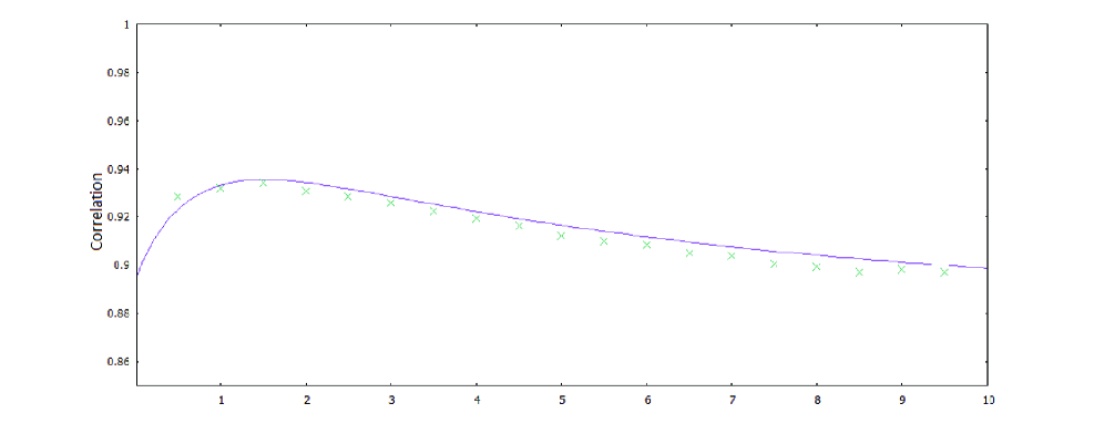
Figure 2: Numerical estimate of the correlation $\rho(x)$ between the FPT and the FPA of BM with drift $-\mu$ starting at $x=10,$ for several values of $\mu.$ On the horizontal axes the values of $\gamma=10\mu;$ the solid line represents the exact curve given by (2.19).

2.1.2 Joint moments of any order

For $m,n\in\mathbb{N},$ we go to study the quantity:

$$V_{m,n}(x):=E\left[\tau(x)^{m}A(x)^{n}\right].$$ (2.20)

Of course, $V_{1,1}(x)=E[\tau(x)A(x)]$ coincides with the function $V(x)$ already studied. Applying $\frac{\partial^{m}}{\partial\lambda_{1}^{m}}\frac{\partial^{n}}{\lambda_{2}^{n}}$ to both members of (2.14), calculating for $\lambda_{1}=\lambda_{2}=0,$ we get that $V_{m,n}(x)$ turns out to be solution to:

$$\frac{1}{2}\frac{d^{2}}{dx^{2}}\left[(-1)^{m+n}V_{m,n}(x)\right]-\mu\frac{d}{dx}\left[(-1)^{m+n}V_{m,n}(x)\right]$$

$$=m(-1)^{m+n}V_{m-1,n}(x)+nx(-1)^{m+n}V_{m,n-1}(x).$$

Thus, rearranging, we obtain the following:

Theorem 2.4

$V_{m,n}(x)=E\left[\tau^{m}(x)A^{n}(x)\right]$ is the solution of the problem:

$$\begin{cases}\frac{1}{2}V^{\prime\prime}_{m,n}(x)-\mu V^{\prime}_{m,n}(x)=-mV_{m-1,n}(x)-nxV_{m,n-1}(x)\\ V_{m,n}(0)=0\\ \lim_{\nu\rightarrow+\infty}V_{m,n}(x)=0\end{cases}.$$ (2.21)

$\Box$

Notice that the two conditions are obtained in the same way as in the case of $V_{1,1}(x).$

By solving (2.21) e.g. for $m=2,\ n=1,$ one finds:

$$V_{2,1}(x)=E\left[\tau^{2}(x)A(x)\right]=\frac{x^{4}}{2\mu^{3}}+\frac{2x^{3}}{\mu^{4}}+\frac{4x^{2}}{\mu^{5}}+\frac{4x}{\mu^{6}},$$

and similar polynomial expressions can be obtained for any $m$ and $n,$ implying that, for $\mu>0,$ the moments $E\left[\tau^{m}(x)A(x)^{n}\right]$ are finite, for all $m$ amd $n.$ As far as the form of the solution $V_{m,n}$ of (2.21) is concerned, the following holds:

Proposition 2.5

For all integers $m,n\geq 0$ the solution of (2.21) is a polynomial of degree $m+2n,$ which vanishes at zero.

Proof.  We already know that $V_{1,0}(x)=E(\tau(x))=x/\mu,\ V_{0,1}(x)=E(A(x))=x/2\mu^{2}+x^{2}/2\mu,$ and $V_{1,1}(x)=E(\tau(x)A(x))=x^{3}/2\mu^{2}+x^{2}/\mu^{3}+x/\mu^{4},$ which are polynomials vanishing at $x=0,$ with degree, respectively, $1,\ 2$ and $3,$ all corresponding to the value $m+2n.$ As for the quantity $V_{0,n}(x)=E(A(x)^{n}),$ by using (2.4) with $U(x)=x,$ we find that it is the solution of

$$\begin{cases}\frac{1}{2}V^{\prime\prime}_{0,n}(x)-\mu V^{\prime}_{0,n}(x)=-nxV_{0,n-1}(x)\\ V_{0,n}(0)=0\\ \lim_{\mu\rightarrow+\infty}V_{0,n}(x)=0,\end{cases}$$

which is, as easily seen, a polynomial of degree $2n;$ in fact, the homogeneous solution of the ODE is $c_{1}+c_{2}e^{2\mu x},$ with $c_{i}$ constants to be determined, while a particular solution is a polynomial of degree $2n,$ vanishing at $x=0.$ Since the conditions imply the constant $c_{i}$ to be zero, the result follows. Now, let us suppose that the thesis is true for $m=0$ and $m=1,$ and $n-1$ in place of $n,$ namely we suppose that $V_{0,n-1}$ and $V_{1,n-1}$ are polynomials with degree, respectively, $2(n-1)$ and $2n-1;$ $V_{1,n}(x)$ turns out to be the solution of:

$$\begin{cases}\frac{1}{2}V^{\prime\prime}_{1,n}(x)-\mu V^{\prime}_{1,n}(x)=-mV_{0,n}(x)-nxV_{1,n-1}(x)\\ V_{1,n}(0)=0\\ \lim_{\nu\rightarrow+\infty}V_{1,n}(x)=0.\end{cases}$$ (2.22)

The homogeneous solution is the same as the previous ODE, while, being the second member a polynomial of degree $degr[-mV_{0,n}(x)-x(n-1)V_{1,n-1}(x)]=2n,$ the particular solution is a polynomial of degree $2n+1,$ vanishing at zero; hence, since the imposed conditions imply that the homogeneous part disappears, the solution $V_{1,n}(x)$ is a polynomial of degree $1+2n,$ which vanishes at zero. Therefore, the thesis is proved for $m=1$ and every $n.$

Suppose now the thesis is true for $V_{h,k}(x)$ with $k\in{\bf N}$ if $h<m$ and $k<n$ if $h=m;$ the inductive step consists in proving the thesis for $V_{m,n}.$ But, as in the preceding case, the solution is given by the usual homogeneous solution (which the conditions require to be zero), plus a polynomial, vanishing at $x=0,$ which has degree $m+2n,$ because the second member of (2.21) is a polynomial wit degree $degr[-mV_{m-1,n}(x)-nxV_{m,n-1}(x)]=m+2n-1.$

$\Box$

In the remaining part of this subsection we present a recursive method to find the polynomials $V_{m,n}(x),$ for any $m$ and $n.$

By using Proposition 2.5, we obtain that for every $m,\ n\in{\bf N},$ there exist real numbers $a_{1}^{(m,n)},\dots,a_{m+2n}^{(m,n)}$ such that

$$V_{m,n}(x)=\sum_{k=1}^{m+2n}a_{k}^{(m,n)}x^{k},$$

and, in analogous way, there exist real numbers $a_{k}^{(m-1,n)}$ for $k=1,\dots,m+2n-1$ and $a_{k}^{(m,n-1)}$ for $k=1,\dots,m+2n-2,$ such that

$$V_{m-1,n}(x)=\sum_{k=1}^{m+2n-1}a_{k}^{(m-1,n)}x^{k}=a_{1}^{(m-1,n)}x+\sum_{k=1}^{m+2n-2}a_{k+1}^{(m-1,n)}x^{k+1},$$

and

$$V_{m,n-1}(x)=\sum_{k=1}^{m+2n-2}a_{k}^{(m,n-1)}x^{k}.$$

By calculating the derivatives involved, the equation in (2.21) can be written as

$$\sum_{k=1}^{m+2n-1}k\left[\frac{1}{2}a_{k+1}^{(m,n)}(k+1)-\mu a_{k}^{(m,n)}\right]x^{k-1}-\mu a_{m+2n}^{(m,n)}(m+2n)x^{m+2n-1}$$

$$=-ma_{1}^{(m-1,n)}x+\sum_{k=1}^{m+2n-2}(-ma_{k+1}^{(m-1,n)}-na_{k}^{(m,n-1)})x^{k+1}.$$

By equaling the coefficients of the two members, we get:

- for constant term,

$$a_{2}^{(m,n)}-\mu a_{1}^{(m,n)}=0;$$

- for term of degree $1,$

$$2\left(\frac{3}{2}a_{3}^{(m,n)}-\mu a_{2}^{(m,n)}\right)=-ma_{1}^{(m-1,n)};$$

- for term of degree $d=2,\dots,m+2n-2,$

$$(d+1)\left(\frac{d+2}{2}a_{d+2}^{(m,n)}-\mu a_{d+1}^{(m,n)}\right)=-ma_{d}^{(m-1,n)}-na_{d-1}^{(m,n-1)};$$

- finally, for term of degree $m+2n-1,$

$$-\mu(m+2n)a_{m+2n}^{(m,n)}=-ma_{m+2n-1}^{(m-1,n)}-na_{m+2n-2}^{(m,n-1)}.$$

In order to obtain a more compact notation, we introduce the three matrices

$A^{(m,n)},\ B^{(m-1,n)},\ C^{(m,n-1)}\in\mathbb{R}^{(m+2n)\times(m+2n)},$ such that

$$A^{(m,n)}_{i,j}=\begin{cases}-i\mu&i=j\\ \frac{1}{2}i(i+1)&j=i+1,\ i<m+2n\\ 0&otherwise\end{cases}$$

and

$$B^{(m-1,n)}=\begin{pmatrix}0&\dots&0\\ .&\dots&0\\ 0&\dots&-mI_{m+2n-1}\end{pmatrix},\ C^{(m,n-1)}=\begin{pmatrix}0&\dots&\dots&0\\ .&0&\dots&0\\ .&.&\dots&0\\ 0&\dots&.&-nI_{m+2n-1},\end{pmatrix},$$

where $I_{k}\in\mathbb{R}^{k\times k}$ is the identity matrix. Denoting by $\underline{a}_{m,n}\in\mathbb{R}^{m+2n}$ the vector of the coefficients of $V_{m,n},$ that is

$$\underline{a}_{m,n}=\left(a_{1}^{(m,n)},\dots,a_{m+2n}^{(m,n)}\right)^{T},$$

the following matrix equation resumes the previous equalities:

$$A^{(m,n)}\underline{a}_{m,n}=B^{(m-1,n)}\begin{pmatrix}0\\ \underline{a}_{m-1,n}\end{pmatrix}+C^{(m,n-1)}\begin{pmatrix}0\\ 0\\ \underline{a}_{m,n-1}\end{pmatrix}.$$

Being $A^{(m,n)}$ invertible, it results

$$\underline{a}_{m,n}=(A^{(m,n)})^{-1}B^{(m-1,n)}\begin{pmatrix}0\\ \underline{a}_{m-1,n}\end{pmatrix}+(A^{(m,n)})^{-1}C^{(m,n-1)}\begin{pmatrix}0\\ 0\\ \underline{a}_{m,n-1}\end{pmatrix}.$$ (2.23)

As it easily seen, the inverse matrix $(A^{(m,n)})^{-1}$ is

$$(A^{(m,n)})^{-1}=\begin{pmatrix}-1/\mu&c_{1,2}&\dots&\dots&\dots&\dots&c_{1,m+2n}\\ 0&-1/2\mu&c_{2,3}&.&\ &\ &.\\ 0&.&.&.&\ &\ &.\\ 0&.&.&-1/i\mu&c_{i,i+1}&\ &.\\ .&.&.&.&.&.&.\\ .&.&.&.&.&\ &c_{m+2n,m+2n-1}\\ 0&.&.&.&.&0&-1/(m+2n)\mu\end{pmatrix},$$

where, for every $i,$

$$c_{i,i+1}=-\frac{1}{2\mu^{2}},$$

and for every $j>i+1,$

$$c_{i,j}=\frac{(i+1)\cdots(j-1)}{2^{j-i}\mu^{j-i+1}}.$$

Now, defining the two new matrices

$$D^{(m-1,n)}:=(A^{(m,n)})^{-1}B^{(m-1,n)}\ {\rm and}\ E^{(m,n-1)}:=(A^{(m,n)})^{-1}C^{(m,n-1)},$$

we have

$$D^{(m-1,n)}_{i,j}=\begin{cases}0&j=1\\ \frac{m}{i\mu}&i=j>1\\ -mc_{i,i+1}=\frac{m}{2\mu^{2}}&j=i+1\\ -mc_{i,j}=m\frac{(i+1)\cdots(j-1)}{2^{j-i}\mu^{j-i+1}}&j>i+1\\ 0&otherwise\end{cases}$$

and

$$E^{(m,n-1)}_{i,j}=\begin{cases}0&j=1,2\\ \frac{m}{i\mu}&i=j>2\\ -nc_{i,i+1}=\frac{n}{2\mu^{2}}&j=i+1,j>2\\ -nc_{i,j}=n\frac{(i+1)\cdots(j-1)}{2^{j-i}\mu^{j-i+1}}&j>i+1,j>2\\ 0&otherwise\end{cases}$$

Finally, (2.23) becomes

$$\underline{a}_{m,n}=D^{(m-1,n)}\begin{pmatrix}0\\ \underline{a}_{m-1,n}\end{pmatrix}+E^{(m,n-1)}\begin{pmatrix}0\\ 0\\ \underline{a}_{m,n-1}\end{pmatrix},$$ (2.24)

which provides a recursive formula to find the coefficients $a_{k}^{(m,n)},\ k=1,\dots,m+2n.$ Thanks to the fact that the involved matrices are triangular, for $m$ and $n$ not too large, (2.24) represents a faster way to obtain the coefficients of the polynomial $V_{m,n}(x),$ than solving directly the ODE (2.21).

2.2 Expected value of the time average till the FPT

In this subsection, we fill find a closed form for

$$E\left(\frac{A(x)}{\tau(x)}\right)=E\left(\frac{1}{\tau(x)}\int_{0}^{\tau(x)}X(t)dt\right),$$

that is the expected value of the time average of drifted BM $X(t)=x-\mu t+B_{t}$ till its FPT below zero.

If $M_{\lambda}(x)=M_{\lambda_{1},\lambda_{2}}(x)$ is the joint Laplace transform of $(A(x),\tau(x)),$ defined by (2.13), we notice that

$$E\left(A(x)e^{\lambda_{1}\tau(x)}\right)=-\lim_{\lambda_{2}\rightarrow 0^{+}}\frac{\partial}{\partial\lambda_{2}}M_{\lambda_{1},\lambda_{2}}(x),$$

and

$$E\left(\frac{A(x)}{\tau(x)}\right)=\int_{0}^{+\infty}E\left(A(x)e^{\lambda_{1}\tau(x)}\right)d\lambda_{1}\ .$$ (2.25)

Thus, the calculation of $E(A(x)/\tau(x))$ is reduced to find $-\lim_{\lambda_{2}\rightarrow 0^{+}}\frac{\partial}{\partial\lambda_{2}}M_{\lambda_{1},\lambda_{2}}(x).$ By taking the partial derivative with respect to $\lambda_{2}$ in (2.14), calculated for $\lambda_{2}=0,$ we easily obtain that $w(x):=E(A(x)e^{-\lambda_{1}\tau(x)})$ is solution to the equation

$$\frac{1}{2}w^{\prime\prime}(x)-\mu w^{\prime}(x)=\lambda_{1}w(x)-xE(e^{-\lambda_{1}\tau(x)}).$$

By recalling the expression of the Laplace transform of $\tau(x),$ that is

$E(e^{-\lambda_{1}\tau(x)})=e^{-x(\sqrt{\mu^{2}+2\lambda_{1}}-\mu)}$ (see (2.5)), and reasoning as before, we obtain that $w(x)$ is the solution of the problem

$$\begin{cases}\frac{1}{2}w^{\prime\prime}(x)-\mu w^{\prime}(x)=\lambda_{1}w(x)-xe^{-x(\sqrt{\mu^{2}+2\lambda_{1}}-\mu)}\\ w(0)=0\\ \lim_{\mu\rightarrow+\infty}w(x)=0.\end{cases}$$ (2.26)

By calculation, we find that the explicit expression of $w(x)$ is:

$$w(x)=E\left[A(x)e^{-\lambda_{1}\tau(x)}\right]=e^{\mu x}e^{-x\sqrt{\mu^{2}+2\lambda_{1}}}\left[\frac{x}{2(\mu^{2}+2\lambda_{1})}+\frac{x^{2}}{2\sqrt{\mu^{2}+2\lambda_{1}}}\right],$$ (2.27)

which coincides with equation (12) of [7], that was derived by using different arguments. Finally, integrating with respect to $\lambda_{1},$ from (2.25) we get that the expected value of the time average of $X$ till its FPT below zero is:

$$E[A(x)/\tau(x)]=\frac{x}{2}\left[1+\int_{0}^{+\infty}\frac{e^{-sx}}{s+\mu}\ ds\right].$$ (2.28)

This result was already obtained in [7] (see eq. (29) therein), as a consequence of (2.25). Notice that $E[A(x)/\tau(x)]$ turns out to be $\geq x/2,$ being $\lim_{\mu\rightarrow+\infty}E[A(x)/\tau(x)]=x/2,$ and $\lim_{\mu\rightarrow 0^{+}}E[A(x)/\tau(x)]=+\infty.$

3 Conclusions and final remarks

In this paper, we have continued the study, already undertook in [1], of the first-passage area (FPA) $A(x),$ swept out by a one-dimensional jump-diffusion process $X(t),$ starting from $x>0,$ till its first-passage time (FPT) $\tau(x)$ below zero. Here, we have investigated the joint distribution of $\tau(x)$ and $A(x),$ in the special case when $X$ is Brownian motion with negative drift $-\mu,$ that is, $X(t)=x-\mu t+B_{t},$ ($B_{t}$ denotes standard Brownian motion). We have established differential equations with boundary conditions for the Laplace transform of the random vector $(\tau(x),A(x)),$ and for the joint moments $E[\tau(x)^{m}A(x)^{n}]$ of the FPT and FPA; moreover, we have presented an algorithm to find recursively $E[\tau(x)^{m}A(x)^{n}],$ for any $m$ and $n.$ In particular, closed formulae for $E[\tau(x)A(x)]$ and then for the correlation between $\tau(x)$ and $A(x),$ were explicitly obtained, which match existing results, obtained by approximation arguments in [7]. Furthermore, we have calculated the expected value of the time average of $X(t)$ till its FPT below zero.

The difference compared to similar articles (see e.g. [7]) is that our results have been obtained without the use of special functions.

We remark that all the results contained in this paper can be extended in principle to the case of a one-dimensional time-homogeneous diffusion $X(t),$ which is the solution of a stochastic differential of the form

$$\begin{cases}dX(t)=b(X(t))dt+\sigma(X(t))dB_{t}\\ X(0)=x>0,\end{cases}$$ (3.1)

where the functions $b(\cdot),\sigma(\cdot)$ satisfy suitable conditions for the existence and uniqueness of the solution of (3.1) (see e.g. [2], [4]). Now, the FPT of $X$ below zero is defined by $\tau(x)=\inf\{t>0:X(t)\leq 0|X(0)=x\}$ and it is required the additional condition that $\tau(x)$ is finite with probability one (this evidently depends on the behavior of the drift $b(x)$ and the diffusion coefficient $\sigma(x)).$ Under this condition, all the differential problems concerning the various quantities considered in Section 2 still hold, provided that $\frac{1}{2}V^{\prime\prime}(x)-\mu V^{\prime}(x)$ is replaced with the infinitesimal operator of $X,$ i.e. $LV(x)=\frac{1}{2}\sigma^{2}(x)V^{\prime\prime}(x)+b(x)V^{\prime}(x).$ Of course, the differential equations obtained in this way are more complicated, since in most cases their solutions cannot be obtained in closed form.

References

- [1] Abundo, M. On the first-passage area of a one-dimensional jump-diffusion process. Methodol Comput Appl Probab 2013, 15, 85- 103. (Online First, April 2011). DOI 10.1007/s11009-011-9223-1.
- [2] Gihman, I.I. and Skorohod, A.V. Stochastic differential equations. Springer-Verlag, Berlin, 1972.
- [3] Grandshteyn, I.S. and Ryzhik, I. M. Tables of Integrals, Series and Products. 5th ed. Academic, London, 1980.
- [4] Ikeda, N. and Watanabe, S. Stochastic differential equations and diffusion processes. North-Holland Publishing Company, 1981
- [5] Janson, S. Brownian excursion area, Wright s constants in graph enumeration, and other Brownian areas. Probability Surveys 2007, 4: 80–145.
- [6] Karlin, S. and Taylor, H.M. A second course in stochastic processes. Academic Press, New York, 1975.
- [7] Kearney, M.J., Pye, A.J., and Martin R.J. On correlations between certain random variables associated with first passage Brownian motion. J. Phys. A: Math and Theor. 2014, 47 (22): 225002. DOI: 10.1088/1751-8113/47/22/225002
- [8] Kearney, M. J. and Majumdar, S.N. On the area under a continuous time Brownian motion till its first-passage time. J. Phys. A: Math. Gen. 2005, 38: 4097–4104.
- [9] Kearney, M. J., Majumdar, S.N. and Martin R.J. The first-passage area for drifted Brownian motion and the moments of the Airy distribution. J. Phys. A: Math. Theor. 2007, 40: F863–F864.
- [10] Knight, F. B. The moments of the area under reflected Brownian Bridge conditional on its local time at zero. Journal of Applied Mathematics and Stochastic Analysis 2000, 13 (2): 99–124.
- [11] Perman, M. and Wellner, J. A. On the Distribution of Brownian Areas. The Annals of Applied Probability 1996, 6 (4) 1091–1111.