Leading Impulse Response Identification
via the Weighted Elastic Net Criterion

Abstract

This paper deals with the problem of finding a low-complexity estimate of the impulse response of a linear time-invariant discrete-time dynamic system from noise-corrupted input-output data. To this purpose, we introduce an identification criterion formed by the average (over the input perturbations) of a standard prediction error cost, plus a weighted $\ell_{1}$ regularization term which promotes sparse solutions. While it is well known that such criteria do provide solutions with many zeros, a critical issue in our identification context is where these zeros are located, since sensible low-order models should be zero in the tail of the impulse response. The flavor of the key results in this paper is that, under quite standard assumptions (such as i.i.d. input and noise sequences and system stability), the estimate of the impulse response resulting from the proposed criterion is indeed identically zero from a certain time index $n_{l}$ (named the leading order) onwards, with arbitrarily high probability, for a sufficiently large data cardinality $N$. Numerical experiments are reported that support the theoretical results, and comparisons are made with some other state-of-the-art methodologies.

, ,

1 Introduction

A large part of the literature on identification of linear time-invariant (LTI) dynamic systems follows a statistical approach (Ljung (1999a); Söderström and Stoika (1989)), where probabilistic assumptions are made, at least on the noise corrupting the measurements. The techniques available in this context may be classified in two main categories: parametric and nonparametric. Parametric techniques are mainly based on the prediction error methods (PEMs) or on the maximum likelihood approach, if Gaussian noise is assumed. The identified models belong to finite-dimensional spaces of given order, like FIR, ARX, ARMAX, OE, Laguerre, Kautz or orthonormal basis function models. In order to limit the model complexity and to avoid possible overfitting, a tradeoff between bias and variance is usually considered, and the model order selection is performed by optimizing some suitable cost function – such as the Akaike’s information criterion AIC (Akaike (1974)), the Rissanen’s Minimum Description Length MDL, or the Bayesian information criterion BIC (Rissanen (1978); Schwarz (1978)) – and by applying some form of cross validation (CV), like hold-out or leave-one-out. Possible limits of these parametric methods have been pointed out in Pillonetto and De Nicolao (2010); Pillonetto et al. (2011); Chen et al. (2012), where it is shown that the sample properties of PEM approaches equipped with, e.g., AIC and CV, may be rather unsatisfactory and quite far from those predicted by standard (i.e., without model selection) statistical theory.

The nonparametric techniques aim to obtain the overall system’s impulse response as a suitable deconvolution of observed input-output data. In particular, very promising approaches have been recently developed, based on results coming from the machine learning field, see, e.g., Pillonetto et al. (2014) and the references therein. Rather than postulating finite-dimensional hypothesis spaces, the estimation problem is tackled in an infinite-dimensional space, and the intrinsical ill-posedness of the problem is circumvented by using suitable regularization methods. In particular, the system’s impulse response is modeled as a zero-mean Gaussian process, and the prior information is introduced by simply assigning a specific covariance, named kernel in the machine learning literature. This procedure can be interpreted as the counterpart of model order selection in the parametric PEM approach and, in some cases, it is shown to be much more robust.

In the present paper, a novel nonparametric method is presented, whereby an estimate of the system’s impulse response is obtained by minimizing a suitable cost function that directly takes into account the resulting model complexity. The aim is indeed to obtain a low-complexity model of the system, in the form of a reduced-order FIR (in this sense, the approach is not so far from parametric techniques). A key feature of the proposed approach, representing a relevant improvement over the state of the art, is that it allows for an effective model order selection, without using strong a-priori information on the true system. More specifically, we propose the use of an identification criterion which is a weighted combination of (a) a standard prediction error term, (b) an $\ell_{2}$ regularization term, and (c) a weighted $\ell_{1}$ penalty term which promotes sparse solutions; a full justification for such criterion is given in Section 3.2. This type of criterion corresponds to the so-called Elastic Net cost, which recently became popular in the machine learning community, see, e.g., Zou and Hastie (2005); De Mol et al. (2009). Notice that, while it is well known that the use of $\ell_{1}$ regularization leads to sparse solutions, sparsity alone is not a very interesting feature in our identification context. Indeed, reduced-order models are obtained only if the sparsity of the solution follows a specific pattern, whereby the zeros are all concentrated in the tail of the impulse response. Obtaining such a pattern is not obvious, nor a-priori granted by the $\ell_{1}$ regularization. One of the key contributions of this paper is to prove that, under standard assumptions, the impulse response estimated via our Elastic-Net type of criterion has the property of being indeed nonzero only on the initial part of the impulse response (which we shall name the leading response), with arbitrarily high probability, if the number of data $N$ is sufficiently large.

The present paper is organized as follows. In Section 2 the notation is set, and some preliminary results on a Chebyshev’s type of convergence for random variables are stated. Section 3 describes the linear identification problem of interest, and contains the derivations of the Elastic Net cost. The main results on the recovery of the leading part of the impulse response are contained in Section 4. Section 5 illustrates a practical procedure for implementing the proposed identification scheme. Numerical experiments, including a comparative discussion with other identification methods, are given in Section 6. All proofs are contained in the Appendix.

2 Notation and preliminaries

2.1 Notation

For a vector $x\in{\ {\mathbb{R}}^{N}}$ , we denote by $[x]_{i}$ the $i$-th entry of $x$, and we define its support as

$$\mathop{\mathrm{supp}}(x)\doteq\{i\in\{1,\ldots,N\}:[x]_{i}\neq 0\}.$$

The notation $\|x\|_{p}$ represents the standard $\ell_{p}$ norm of $x$, and $\|x\|_{0}$ denotes the cardinality of $\mathop{\mathrm{supp}}(x)$, that is the number of nonzero entries of $x$.

For a matrix $X\in{{\mathbb{R}}^{N,M}}$ (with $M$ possibly equal to $\infty$), we denote by $[X]_{i,j}$ the entry of $X$ in row $i$ and column $j.$ For $n\leq M$, we denote by $X_{\uparrow n}\in{{\mathbb{R}}^{N,n}}$ the sub-matrix formed by the first $n$ columns of $X$, with $X_{\downarrow n}\in{{\mathbb{R}}^{N,M-n}}$ the sub-matrix formed by the columns of $X$ of indices $n+1,\ldots,M$, and with $X_{\sharp n}$ the $n\times n$ principal sub-matrix of $X$. The identity matrix is denoted by $I$, or by $I_{n}$, if we wish to specify its dimension. We denote by $X^{\dagger}$ the Moore-Penrose pseudo-inverse of $X$; if $X$ has full column rank, then $X^{\dagger}=(X^{\top}X)^{-1}X^{\top}$.

If $x$ is a random variable, then $\mathbb{E}\{x\}$ denotes the expected value of $x$, and ${\mathrm{var}}\{x\}$ denotes its variance: ${\mathrm{var}}\{x\}=\mathbb{E}\{(x-\mathbb{E}\{x\})^{2}\}$. $\mathbb{P}$ denotes a probability measure on $x$. The symbol $\leadsto$ implies almost sure convergence, and it is formally defined in Section 2.2.1.

2.2 Chebyshev’s inequality for certain empirical means

Let $x_{i}$, $i=1,\ldots,$ be a sequence of (not necessarily independent) random variables such that $\mathbb{E}\{x_{i}\}=\mu<\infty$ for all $i$, ${\mathrm{var}}\{x_{i}\}=\sigma_{i}^{2}\leq\overline{\sigma}^{2}<\infty$ for all $i$, and $\mathbb{E}\{(x_{i}-\mu)(x_{j}-\mu)\}=0$ for all $i\neq j$. For given $N\geq 1$, define the empirical mean

$$\hat{x}_{N}\doteq\tfrac{1}{N}\mathop{\textstyle\sum}\nolimits_{i=1}^{N}x_{i}.$$

Obviously, from linearity of the expectation, it holds that $\mathbb{E}\{\hat{x}_{N}\}=\mu$. Further, we have that

$$\sigma^{2}\!\doteq\mathrm{var}\{\hat{x}_{N}\}\!=\!\mathbb{E}\!\left\{\!(\hat{x}_{N}\!-\!\mu)^{2}\right\}\!=\!\frac{1}{N^{2}}\mathbb{E}\!\left\{\!\left[\mathop{\textstyle\sum}\nolimits_{i=1}^{N}(x_{i}\!-\!\mu)\!\right]^{\!2}\right\}$$

$$= \!\frac{1}{N^{2}}\!\!\left[\rule[0.0pt]{0.0pt}{14.22636pt}\right.\mathop{\textstyle\sum}_{i=1}^{N}\!\mathbb{E}\!\left\{\!(x_{i}\!-\!\mu)^{2}\right\}\!+\!\!\mathop{\textstyle\sum}_{i=1}^{N}\mathop{\textstyle\sum}_{j=1,\,j\neq i}^{N}\!\mathbb{E}\left\{(x_{i}\!-\!\mu)(x_{j}\!-\!\mu)\right\}\left.\rule[0.0pt]{0.0pt}{14.22636pt}\right]$$

$$= \mathop{\textstyle\sum}\nolimits_{i=1}^{N}\left.\sigma_{i}^{2}\right/N^{2}\leq\left.\overline{\sigma}^{2}\right/N,$$

where the last passages follow from the fact that the $x_{i}$s are uncorrelated, and have first moment $\mu$ and variance $\sigma_{i}^{2}\!\leq\!\overline{\sigma}^{2}$. Chebyshev’s inequality applied to the random variable $\hat{x}_{N}$ thus states that, for any $\eta\!>\!0$,

$$\mathbb{P}\{|\hat{x}_{N}-\mu|\geq\eta\sigma\}\leq{1}/{\eta^{2}}.$$ (1)

Since $\eta\sigma\leq\eta\overline{\sigma}/\sqrt{N}$, we have that $\mathbb{P}\{|\hat{x}_{N}-\mu|\geq\eta\overline{\sigma}/\sqrt{N}\}\leq\mathbb{P}\{|\hat{x}_{N}-\mu|\geq\eta\sigma\}$, whence, from (1), we obtain that $\mathbb{P}\{|\hat{x}_{N}-\mu|\geq\eta\overline{\sigma}/\sqrt{N}\}\leq{1}/{\eta^{2}}$. Equivalently, we can state that, for any $\epsilon>0$, it holds that

$$\mathbb{P}\{|\hat{x}_{N}-\mu|\geq\epsilon\}\leq\left.\overline{\sigma}^{2}\right/\left(N\epsilon^{2}\right).$$

We thus conclude that, for any given accuracy $\epsilon>0$ and probability $\beta\in(0,1)$, it holds that

$$\mathbb{P}\{|\hat{x}_{N}-\mu|\geq\epsilon\}\leq\beta,\quad\forall N\geq\left\lceil\left.\overline{\sigma}^{2}\right/\left(\beta\epsilon^{2}\right)\right\rceil.$$

Notice that (1) implies that $\mathbb{P}\{|\hat{x}_{N}-\mu|>\eta\sigma\}\leq{1}/{\eta^{2}}$; hence, by considering the complementary event, it also holds that $\mathbb{P}\{|\hat{x}_{N}-\mu|\leq\eta\sigma\}\geq 1-{1}/{\eta^{2}}$, from which it follows that

$$\mathbb{P}\{|\hat{x}_{N}-\mu|\leq\epsilon\}\geq 1-\left.\overline{\sigma}^{2}\right/\left(N\epsilon^{2}\right).$$

2.2.1 Meaning of the convergence symbol $\leadsto$

For a random variable $z_{N}$ that depends on $N$ and for a given real value $\bar{z}$, the notation $z_{N}\leadsto\bar{z}$ means that for any given $\epsilon>0$ and $\beta\in(0,1)$ there exists a finite integer $N_{\epsilon,\beta}$ such that

$$\mathbb{P}\{|z_{N}-\bar{z}|\geq\epsilon\}\leq\beta,\quad\forall N\geq N_{\epsilon,\beta}.$$ (2)

Notice that $z_{N}\leadsto\bar{z}$ implies that $z_{N}$ converges to $\bar{z}$ almost surely (that is, with probability one), as $N$ tends to infinity. However, we are specifically interested in the property in (2), that holds for possibly large, but finite, $N\!$.

2.3 Lipschitz functions of random variables

If $z_{N}$ is the empirical mean of $N$ uncorrelated variables with common mean $\mu$ and variance bounded by $\overline{\sigma}^{2}$ then, from the discussion in Section 2.2, we conclude that indeed $z_{N}\leadsto\mu$ and, in particular, (2) holds for $N_{\epsilon,\beta}=\left\lceil\left.\overline{\sigma}^{2}\right/\left(\beta\epsilon^{2}\right)\right\rceil$. However, we shall use the convergence notation $z_{N}\leadsto\bar{z}$ also when $\bar{z}$ is not necessarily the expected value of $z_{N}$, and/or when $z_{N}$ is not necessarily an empirical mean. The following lemma holds.

Lemma 1.

For any fixed integer $p$, let $y_{1},\ldots,y_{p}$ be (possibly correlated) scalar random variables that depend on $N$ and such that $y_{i}\leadsto\bar{y}_{i}$, $i=1,\ldots,p$, for some given values $\bar{y}_{1},\ldots,\bar{y}_{p}$. Let $f$ be a Lipschitz continuous function from ${\ {\mathbb{R}}^{p}}$ into ${\ {\mathbb{R}}}$, such that $f(\bar{y}_{1},\ldots,\bar{y}_{p})$ is finite. Then, it holds that $f(y_{1},\ldots,y_{p})\leadsto f(\bar{y}_{1},\ldots,\bar{y}_{p})$.

 

Appendix A.1 contains a proof of Lemma 1.

3 Problem setup

3.1 A linear measurement model

We consider an identification experiment in which a discrete-time scalar input signal $\tilde{u}(k)$ enters an LTI dynamic system, which produces in response a scalar output signal $\tilde{y}(k)$. This output is acquired via noisy measurements over a time window $k=1,\ldots,N$, obtaining a sequence of output measurements $y(k)=\tilde{y}(k)+\delta_{y}(k)$, $k=1,\ldots,N$, where $\delta_{y}(k)$ is the measurement noise sequence. Since the unknown system is assumed to be LTI, there exists a linear relation between the output measurements and the unknown system’s impulse response $h(i)$, $i=1,\ldots$ Assuming that the system is operating in steady state, this relation is given by the discrete-time convolution: for $k=1,\ldots,N$,

$$y(k)\!=\!\tilde{y}(k)+\delta_{y}(k)\!=\!\!\mathop{\textstyle\sum}_{i=1}^{\infty}\!\tilde{u}(k-i+1)h(i)+\delta_{y}(k).$$ (3)

Observe that, following a nonparametric approach, we do not assume to know in advance the order of the unknown system; therefore, in (3), all values $h(i)$ can be, a priori, nonzero. Letting

$$y\!\doteq\!\left[\!\begin{array}[]{c}\vspace*{-7.0mm}\hfil\\ y(1)\vspace*{-2.0mm}\\ y(2)\vspace*{-2.5mm}\\ \vdots\vspace*{-2.5mm}\\ y(N)\vspace*{-0.5mm}\end{array}\!\right]\!;\;\;\delta_{y}\!\doteq\!\left[\!\begin{array}[]{c}\vspace*{-7.0mm}\hfil\\ \delta_{y}(1)\vspace*{-2.0mm}\\ \delta_{y}(2)\vspace*{-2.5mm}\\ \vdots\vspace*{-2.5mm}\\ \delta_{y}(N)\vspace*{-0.5mm}\end{array}\!\right]\!;\;\;\tilde{u}_{i}\!\doteq\!\left[\!\begin{array}[]{c}\vspace*{-7.0mm}\hfil\\ \tilde{u}(2-i)\vspace*{-2.0mm}\\ \tilde{u}(3-i)\vspace*{-2.5mm}\\ \vdots\vspace*{-2.5mm}\\ \tilde{u}(N+1-i)\vspace*{-0.5mm}\end{array}\!\right]\!,$$

for $i=1,2,\ldots,$ we can write (3) in vector format as

$$y=\mathop{\textstyle\sum}\nolimits_{i=1}^{\infty}\tilde{u}_{i}h(i)+\delta_{y}.$$ (4)

For any integer $n\geq 0$, we define

$$\tilde{U}_{\uparrow n}\doteq[\tilde{u}_{1}\,\cdots\,\tilde{u}_{n}]\in{\!{\mathbb{R}}^{N,n}},\;\;h_{\uparrow n}\doteq[h(1)\,\cdots\,h(n)]^{\top}{\!}\in{\!{\mathbb{R}}^{n}},$$

as well as the semi-infinite matrices and vectors

$$\begin{array}[]{l}\tilde{U}_{\downarrow n}\doteq[\tilde{u}_{n+1}\;\tilde{u}_{n+2}\;\cdots]\in{\!{\mathbb{R}}^{N,\infty}},\rule[-7.11317pt]{0.0pt}{7.11317pt}\vspace*{-0.5em}\\ h_{\downarrow n}\doteq[h(n+1)\;h(n+2)\;\cdots]^{\top}{\!}\in{\!{\mathbb{R}}^{\infty}}.\end{array}$$

Let now $q\leq N$ be a given integer: our goal is to estimate the first $q$ elements of the impulse response $h$ (i.e., to estimate $h_{\uparrow q}\in{{\mathbb{R}}^{q}}$), from $N$ noisy output measurements. The value of $q$ is fixed by the decision maker, based on the available number of measurements $N$ and on a priori knowledge. For instance, under a standard assumption of stability (see Assumption 2), since $h(i)$ decays exponentially, one may a priori assess that the response will be negligible for $i\geq q$, for some sufficiently large $q$. We can then rewrite (4) as

$$y=\tilde{U}_{\uparrow q}h_{\uparrow q}+\delta_{y}+y{{}^{\mathrm{ud}}},$$

where

$$y{{}^{\mathrm{ud}}}\doteq\tilde{U}_{\downarrow q}h_{\downarrow q}$$

represents the unmodelled dynamics due to the truncation of the impulse response to the $q$-th term. For simplifying the notation, we let from now on

$$\tilde{U}\doteq\tilde{U}_{\uparrow q},$$

which is an $N\times q$ Toeplitz matrix.

3.2 An Elastic Net identification criterion

The initial approach that we consider for identifying the unknown system’s impulse response consists in finding an estimate of $h_{\uparrow q}$ that minimizes w.r.t. $x$ the cost function

$$\hskip 71.13188pt\frac{1}{\gamma}\|y-\tilde{U}x\|_{2}^{2}+\|x\|_{0},$$ (5)

where $\gamma>0$ is a suitable tradeoff parameter. The first term in (5) is the standard prediction error, while the second term $\|x\|_{0}$ represents the cardinality of $x$, that is the number of nonzero entries in $x$. This term penalizes the complexity of the estimate, thus promoting solutions with a small number of nonzero entries. Note incidentally that, if $\delta_{y}(k)$ is a sequence of independent identically distributed (i.i.d.) Normal random variables with zero mean and known variance $\sigma_{y}^{2}$ then, for $\gamma=2\sigma_{y}^{2}$, the above criterion coincides with the well-known Akaike’s information criterion AIC. Other standard criteria, such as the BIC, can also be obtained for different values of $\gamma$.

3.2.1 Input uncertainty and averaged cost

In a realistic identification experiment, however, the input signal $\tilde{u}(k)$ that enters the unknown system is a possibly “perturbed” version of a nominal input signal $u(k)$ that the user intends to provide to the system. To model this situation, we assume that $\tilde{u}(k)=u(k)+\delta_{u}(k)$, where $u(k)$ is the nominal input signal, and $\delta_{u}(k)$ is an i.i.d. random noise sequence, which is assumed to have zero mean and variance $\sigma_{u}^{2}$ (setting $\sigma_{u}^{2}=0$ we recover the standard, no-input-noise, situation). Considering the time window $k=1,\ldots,N$, we have in matrix form that

$$\tilde{U}=U+\Delta,$$ (6)

where $U$ is an $N\times q$ Toeplitz matrix containing the nominal input signal, and $\Delta$ is an $N\times q$ Toeplitz matrix containing the noise samples $\delta_{u}(k)$. Specifically, $U\doteq[u_{1}\,\cdots\,u_{q}]$, and $\Delta\doteq[\delta_{1}\,\cdots\,\delta_{q}]$, where for $i=1,\ldots,q$

$$u_{i}\doteq\left[\begin{array}[]{c}\vspace*{-7.0mm}\hfil\\ u(2-i)\vspace*{-2.0mm}\\ u(3-i)\vspace*{-3.0mm}\\ \vdots\vspace*{-2.0mm}\\ u(N+1-i)\vspace*{-0.5mm}\end{array}\right],\quad\delta_{i}\doteq\left[\begin{array}[]{c}\vspace*{-7.0mm}\hfil\\ \delta_{u}(2-i)\vspace*{-2.0mm}\\ \delta_{u}(3-i)\vspace*{-3.0mm}\\ \vdots\vspace*{-2.0mm}\\ \delta_{u}(N+1-i)\vspace*{-0.5mm}\end{array}\right].$$

We account for input uncertainty in the identification experiment by “averaging” the effect of this uncertainty in the cost criterion (5). This leads to the following cost function:

$$\hskip 14.22636ptJ_{0}(x) = \mathbb{E}_{\delta_{u}}\left\{\frac{1}{\gamma}\|y-\tilde{U}x\|_{2}^{2}+\|x\|_{0}\right\}$$ (7)

$$= \frac{1}{\gamma}\mathbb{E}_{\delta_{u}}\left\{\|y-(U+\Delta)x\|_{2}^{2}\right\}+\|x\|_{0},$$

where $\mathbb{E}_{\delta_{u}}$ denotes expectation w.r.t. the random sequence $\delta_{u}$. Elaborating on the expression (7), we obtain

$$\mathbb{E}_{\delta_{u}}\{\|y-(U+\Delta)x\|_{2}^{2}\}$$

$$= \mathbb{E}_{\delta_{u}}\{\|y-Ux\|_{2}^{2}+\|\Delta x\|_{2}^{2}-2(y-Ux)^{\top}\Delta x\}$$

$$= \|y-Ux\|_{2}^{2}+\mathbb{E}_{\delta_{u}}\{\|\Delta x\|_{2}^{2}\}$$

$$= \|y-Ux\|_{2}^{2}+x^{\top}\mathbb{E}_{\delta_{u}}\{\Delta^{\top}\Delta\}x,$$

because $\mathbb{E}_{\delta_{u}}\{\Delta\}=0$. Since $\delta_{u}(k)$ is an i.i.d. sequence, and since $\Delta$ has Toeplitz structure, it is easy to verify that the off-diagonal terms in $\mathbb{E}_{\delta_{u}}\{\Delta^{\top}\Delta\}$ are zero, while the diagonal terms are all equal to $N\sigma_{u}^{2}$. Therefore, it holds that $\mathbb{E}_{\delta_{u}}\{\Delta^{\top}\Delta\}=N\sigma_{u}^{2}I_{q}$, and the expected cost $J_{0}(x)$ is explicitly expressed as

$$J_{0}(x)=\frac{1}{\gamma}\|y-Ux\|_{2}^{2}+\frac{N\sigma_{u}^{2}}{\gamma}\|x\|_{2}^{2}+\|x\|_{0}.$$ (8)

Notice that this setting can be easily extended to wide-sense stationary input noise sequences $\delta_{u}(k)$, in which case the second term in the above expression takes the form $\frac{N}{\gamma}x^{\top}R_{u}x$, where $R_{u}$ is the autocorrelation matrix of $\delta_{u}$. For simplicity, however, we here focus on the basic case of an i.i.d. sequence, for which $R_{u}=\sigma_{u}^{2}I_{q}$. Observe further that accounting for noise on the input signal results in the introduction of a Tikhonov-type regularization term in (8), a fact that has been previously observed in other contexts such as neural network training, see, e.g., Bishop (1995).

3.2.2 Normalizing the variables

We next rescale the variables in the cost (8) by normalizing the columns of the regression matrix. First, we rewrite $J_{0}(x)$ as

$$\hskip 56.9055ptJ_{0}(x)=\frac{1}{\gamma}\left\|b-\bar{A}x\right\|_{2}^{2}+\|x\|_{0},$$ (9)

where

$$b\doteq\left[\begin{array}[]{c}\vspace*{-7.0mm}\hfil\\ y\vspace*{-1.5mm}\\ 0\vspace*{-0.5mm}\end{array}\right],\quad\bar{A}\doteq\left[\begin{array}[]{c}\vspace*{-7.0mm}\hfil\\ U\vspace*{-1.5mm}\\ \sigma_{u}\sqrt{N}I_{q}\vspace*{-0.5mm}\end{array}\right].$$ (10)

Second, we let $T\doteq\mbox{diag}(\|\bar{a}_{1}\|_{2},\ldots,\|\bar{a}_{q}\|_{2})^{-1}$, where $\bar{a}_{i}$ denotes the $i$-th column of $\bar{A}$, and perform the change of variable $\tilde{x}=T^{-1}x$, thus the right-hand side of (9) becomes

$$\tilde{J}_{0}(\tilde{x})\doteq\frac{1}{\gamma}\|b-A\tilde{x}\|_{2}^{2}+\|\tilde{x}\|_{0},$$ (11)

where we defined $A\doteq\bar{A}T$, and we used the fact that $\|T\tilde{x}\|_{0}=\|\tilde{x}\|_{0}$, since the cardinality of a vector does not depend on (nonzero) scalings of the entries of the vector. We observe that the columns $a_{1},\ldots,a_{q}$ of $A$ now have unit Euclidean norm. We let $\tilde{x}_{0}^{*}\doteq\arg\min\,\tilde{J}_{0}(\tilde{x})$, and $x_{0}^{*}\doteq\arg\min\,J_{0}(x)$, where it obviously holds that $x_{0}^{*}=T\tilde{x}_{0}^{*}$. These optimal solutions are hard to determine numerically in practice. However, we do not need to compute them, we only need them for theoretical purposes.

3.2.3 Weighted $\ell_{1}$ relaxation of the cost function

We now introduce the following tractable relaxation of the cost (11):

$$\tilde{J}_{1}(\tilde{x})\doteq\frac{1}{\gamma}\|b-A\tilde{x}\|_{2}^{2}+\|W\tilde{x}\|_{1}.$$ (12)

where $W\doteq\mathop{\mathrm{d}iag}(w_{1},\ldots,w_{q})$ is a suitable weighting matrix, with $\max_{k=1,\ldots,q}w_{k}=1$, $\min_{k=1,\ldots,q}w_{k}>0$. We shall henceforth assume that the weight sequence is nondecreasing: $w_{1}\leq w_{2}\leq\cdots\leq w_{q}=1$.

Notice that, expanding the squared norm in (12), we obtain the cost function $\tilde{J}_{1}$ in the form

$$\tilde{J}_{1}(\tilde{x})=\frac{1}{\gamma}\|y-UT\tilde{x}\|_{2}^{2}+\frac{N\sigma_{u}^{2}}{\gamma}\|T\tilde{x}\|_{2}^{2}+\|W\tilde{x}\|_{1},$$ (13)

which corresponds to the cost expressed in the original variable $x=T\tilde{x}$

$$J_{1}(x)=\frac{1}{\gamma}\|y-Ux\|_{2}^{2}+\frac{N\sigma_{u}^{2}}{\gamma}\|x\|_{2}^{2}+\|WT^{-1}x\|_{1}.$$ (14)

The cost function (13) is strongly convex, hence the optimal solution $\tilde{x}_{1}^{*}\doteq\arg\min\,\tilde{J}_{1}(\tilde{x})$ is unique and, equivalently, the minimization of (14) has a unique optimal solution $x_{1}^{*}=T\tilde{x}_{1}^{*}$. In the following section, we shall study the properties of $x_{1}^{*}$ as an estimate of the impulse response $h_{\uparrow q}$. Note that only two parameters ($\gamma$ and $\sigma_{u}$) have to be chosen to obtain this estimate. A systematic procedure is proposed in Section 5, allowing an effective choice of these parameters, based on the desired trade-off between model complexity and accuracy.

Remark 1.

The cost criterion appearing in (13) is a particular version of the Lasso (see, e.g., Tibshirani (1996)), known as the Elastic Net (Zou and Hastie (2005)). The Elastic Net criterion includes an $\ell_{2}$ regularization term which provides shrinkage and improves conditioning of the $\ell_{2}$-error cost (by guaranteeing strong convexity of the cost), as well as an $\ell_{1}$ penalty term which promotes sparsity in the solution. Elastic Net-based methods are widely used in statistics and machine learning, see, e.g., De Mol et al. (2009); Hastie et al. (2009), and are amenable to very efficient large-scale solution algorithms (Friedman et al. (2010)). To the best of the authors’ knowledge, this is the first work in which the Elastic Net criterion is used in the context of a system identification problem and the resulting sparsity pattern is rigorously analyzed.

4 Leading response recovery

This section contains the main results of the paper. First, we report a preliminary technical lemma (Lemma 2) stating that, under a certain condition, the minimizer $x_{1}^{*}$ of (14) is supported on $\{1,\ldots,n\}$, with $n\leq q$. Second, under some suitable assumptions on the input and noise signals, we show (Theorem 4) that if the unknown system is stable, then for a sufficiently large $N$ and for a given $n\leq q$, there exist explicitly given $\gamma$ values for which the support of $x_{1}^{*}$ is contained in $\{1,\ldots,n\}$, with any given high probability. This means that the estimated impulse response $x_{1}^{*}$ is not only sparse but, with high probability, it is zero precisely on the tail of the system’s impulse response $h_{\uparrow q}$. We next define the notions of leading response and leading support of the system’s impulse response, and show (Corollary 5) that if the unknown system is stable, then for a suitable $\gamma$ and a sufficiently large $N$ the support of $x_{1}^{*}$ is contained in the leading support, with any given high probability; we call this property leading response recovery (LRR). Finally, we show (Corollary 6) that if the true unknown system is FIR then, for a sufficiently large $N$ and for any $\gamma>0$, the estimated impulse response $x_{1}^{*}$ will be sparse, and of order no larger than the order of the true system, with high probability.

4.1 Preliminary results, assumptions and definitions

With the notation set in Section 3.2.2, for a given integer $n\leq q$, let $P_{n}\doteq A_{\uparrow n}A_{\uparrow n}^{\dagger}$ denote the orthogonal projector onto the span of $A_{\uparrow n}$, and define the $n$-leading recovery coefficient $\Upsilon_{n}(A)\doteq 1-\max_{n<i\leq q}w_{i}^{-1}\left\|W_{\sharp n}A_{\uparrow n}^{\dagger}a_{i}\right\|_{1}$, where $a_{i}$ is the $i$-th column of $A$. The following technical lemma, based on a result in Tropp (2006), holds.

Lemma 2.

Suppose that for some integer $n\leq q$ it holds that

$$\left\|W^{-1}A^{\top}(b-P_{n}b)\right\|_{\infty}\leq\gamma\left.\Upsilon_{n}(A)\right/2,$$ (15)

and let $x_{1}^{*}$ be the minimizer of (14). Then, it holds that

$$\mathop{\mathrm{supp}}(x_{1}^{*})\subseteq\{1,\ldots,n\}.$$

 

See Appendix A.2 for a proof of Lemma 2.

Let us now state the following working assumptions.

Assumption 1 (on input and disturbance sequences ).

1. The input $u(k)$ is an i.i.d. sequence with zero mean, bounded variance $\nu^{2}$ and bounded $4$-th order moment $\mathbb{E}\left\{u(k)^{4}\right\}=\overline{m\rule{0.0pt}{5.69054pt}_{4}}\,$.

2. The noise $\delta_{y}(k)$ is an i.i.d. sequence with zero mean and bounded variance $\sigma_{y}^{2}\,$.

3. The input perturbation $\delta_{u}(k)$ is an i.i.d. sequence with zero mean and bounded variance $\sigma_{u}^{2}\,$.

4. $u(k)$, $\delta_{y}(k)$, and $\delta_{u}(k)$ are mutually uncorrelated.

Assumption 2 (Stability ).

The unknown system’s impulse response $h$ is such that $|h(i)|\leq L\rho^{i-1}$, for $i=1,2,\ldots,$ for some given finite $L>0$ and $\rho\in(0,1)$.

We next establish a preliminary lemma.

Lemma 3.

Under Assumption 1, for any pair of column vectors $u_{i}$ and $u_{j}$ it holds that

$$\tfrac{1}{N}u_{i}^{\top}u_{j}\leadsto\left\{\begin{array}[]{l}\vspace*{-7.5mm}\\ \nu^{2}\quad\mbox{if }i=j\vspace*{-2.0mm}\\ 0\quad\mbox{otherwise,}\vspace*{-1.5mm}\end{array}\right.$$ (16)

where the notation $\leadsto$ has the meaning specified in Section 2.2.1. Also, it holds that

$$\hskip 62.59605pt\tfrac{1}{N}u_{i}^{\top}\delta_{y}\leadsto 0,\quad\forall i$$ (17)

$$\hskip 71.13188pt\tfrac{1}{N}u_{i}^{\top}\delta_{j}\leadsto 0,\quad\forall i,j.$$ (18)

 

Appendix A.3 contains a proof of Lemma 3.

We next define the notion of leading order of the system’s impulse response, and the associated notions of leading response and leading support.

Definition 1.

Let Assumption 2 hold. We define the leading order, $n_{l}(N)$, of $h$ as the largest integer $i\leq q$ such that

$$L\rho^{i-1}\geq\frac{\sigma_{y}}{\nu}\times\frac{1}{\sqrt{N}}.$$ (19)

The leading response is $\{h(i),\,i=1,\ldots,n_{l}\}$ and the leading support is $\{1,\ldots,n_{l}\}$.

Remark 2.

We provide an intuitive interpretation of the definition in (19). The leading order is a value such that for time values larger than it the system’s impulse response cannot essentially be discriminated from noise. Indeed, if a classical output error criterion would be used for estimating $h_{\uparrow q}$, then the covariance matrix of the estimated parameter would be of the form ${\sigma_{y}^{2}}(U^{\top}U)^{-1}$, which tends to ${\sigma_{y}^{2}}/({\nu^{2}N})I_{q}$ as $N\to\infty$, see the proof of Theorem 4 for details. The standard error on the generic element $h(i)$ of the impulse response thus goes to zero as $1\!/\!\sqrt{\!N}$, where $N$ is the number of measurements and the proportionality constant $\sigma_{\!y}/_{\!}\nu$ is the noise-to-signal ratio.
The leading order $n_{l}$ is therefore defined as the time value after which the upper bound on $|h(i)|$ goes below the level $\eta=\frac{\sigma_{y}}{\nu}\frac{1}{\sqrt{N}}$, and hence $h(i)$ becomes essentially indistinguishable from noise, for all $i>n_{l}$; if this condition is not met for $i\leq q$, then we just set $n_{l}=q$. It is an immediate consequence of (19) that the leading order grows as the logarithm of $N$, until it saturates to $q$:

$$n_{l}(N)=\min\left(\left\lfloor\frac{\log(\nu L)+\frac{1}{2}\log N-\log(\sigma_{\!y}\rho)}{\log(\rho^{-1})}\right\rfloor,q\right).\text{\vspace*{-0.2em}}$$

4.2 Main results

We next establish the main results of this paper.

Theorem 4.

Let Assumptions 1 and 2 hold. Let $n\leq q$, $\kappa\doteq\nu/\sqrt{\nu^{2}+\sigma_{u}^{2}}$, and

$$\gamma=2\mu w_{n}^{-1}L\rho^{n}\nu\kappa\times\sqrt{N}\text{,}$$ (20)

for some $\mu>1$. Then, for any given $\beta\in(0,1)$ there exists a finite integer $N_{\beta}$ such that for any $N\geq N_{\beta}$ it holds that

$$\mathop{\mathrm{supp}}(x_{1}^{*})\subseteq\{1,\ldots,n\}$$

with probability no smaller than $1-\beta$, where $x_{1}^{*}$ is the minimizer of (14).

 

Appendix A.4 contains a proof of Theorem 4. The key point of this theorem is that if the tradeoff parameter $\gamma$ is chosen proportional to $\sqrt{N}$ then, with high probability and for a sufficiently large $N$, the minimization of (14) provides a solution which is not only sparse, but its sparsity pattern is identically zero on the tail of the impulse response, i.e., the estimated impulse response $x_{1}^{*}$ is FIR of order at most $n$.

A consequence of Theorem 4 is stated in the following corollary: for a suitable constant value of $\gamma$, the minimizer $x_{1}^{*}$ of (14) has its support contained in the leading support.

Corollary 5 (Leading support recovery ).

Let Assumptions 1 and 2 hold. Let $\kappa\doteq\nu/\sqrt{\nu^{2}+\sigma_{u}^{2}}$, and

$$\gamma>2w_{n_{l}(N)}^{-1}\rho\sigma_{y}\kappa.$$ (21)

Then, for any given $\beta\in(0,1)$ there exists a finite integer $N_{\beta}$ such that for any $N\geq N_{\beta}$ it holds that

$$\mathop{\mathrm{supp}}(x_{1}^{*})\subseteq\{1,\ldots,n_{l}(N)\}$$

with probability no smaller than $1-\beta$, where $x_{1}^{*}$ is the minimizer of (14), and $n_{l}(N)$ is the leading order of the unknown system’s impulse response.

 

See Appendix A.5 for a proof of Corollary 5. Corollary 5 states that, under suitable conditions, an estimate of the impulse response based on the minimization of (14) is supported inside the leading support of the system, with high probability. The following corollary provides a similar result, for the case in which the true system is a-priori known to have finite impulse response (FIR).

Corollary 6 (FIR recovery ).

Let Assumption 1 hold. Further, assume the “true,” unknown, system is FIR of order $n\leq q$, with $n$ unknown. Then, for any $\gamma>0$ and for any given $\beta\in(0,1)$ there exists a finite integer $N_{\beta}$ such that for any $N\geq N_{\beta}$ it holds that $\mathop{\mathrm{supp}}(x_{1}^{*})\subseteq\{1,\ldots,n\}$ with probability no smaller than $1-\beta$, where $x_{1}^{*}$ is the minimizer of (14).

 

See Appendix A.6 for a proof of Corollary 6. The key point of this corollary is that if the true system is known to be FIR, then the minimizer of (14) will tendentially recover the true order of the system, regardless of the value of $\gamma\!>\!0$ (but, of course, the larger the value of $\gamma$, the sooner w.r.t. $N$ the condition (15) will be satisfied).

5 Identification procedure

We next formalize a possible procedure illustrating how the proposed methodology can be used in a practical experimental setting. Suppose that a set of data $\{y(k),u(k)\}_{k=3-q}^{N}$ is available from a process of the form (3). Identification of the impulse response $h(i)$ is performed by minimizing the cost function (14). This operation requires the choice of two parameters ($\gamma$ and $\sigma_{u}$). If $\sigma_{u}$ and $\sigma_{y}$ are known from some a-priory information on the noises affecting the system or can be reliably estimated, then $\gamma$ can be chosen according to (21), where $\rho$ can be estimated by means of the technique in Milanese et al. (2010) (see Section 6.1). If instead this information is not available, a systematic procedure for the choice of $\gamma$ and $\sigma_{u}$ is the following one:

• Take “reasonable” sets $\Gamma=\{\gamma^{(1)},\gamma^{(2)},...\}$ and $\Sigma_{u}=\{\sigma_{u}^{(1)},\sigma_{u}^{(2)},...\}$ for $\gamma$ and $\sigma_{u}$ values, respectively. If $\sigma_{u}$ is known from some a-priory information on the noise affecting the input, then $\Sigma_{u}=\sigma_{u}$.

• Define $y$, $U$ and $T$ as shown in Section 3.

• Run the following algorithm:

  $$\begin{array}[]{l}\vspace*{-3.0em}\\ \text{for }i=1:\text{length}(\Sigma_{u})\vspace*{-1.0mm}\\ \qquad\text{for }j=1:\text{length}(\Gamma)\vspace*{-1.0mm}\\ \qquad\qquad\sigma_{u}=\sigma_{u}^{(i)};\ \gamma=\gamma^{(j)};\vspace*{-1.0mm}\\ \qquad\qquad x^{*}(i,j)=\arg\min_{x}J_{1}(x);\vspace*{-1.0mm}\\ \qquad\qquad E(i,j)=\left\|y-Ux^{*}(i,j)\right\|_{2}^{2};\vspace*{-1.0mm}\\ \qquad\qquad C(i,j)=\left\|x^{*}(i,j)\right\|_{0};\vspace*{-1.0mm}\\ \qquad\text{end}\vspace*{-1.0mm}\\ \qquad\text{plot}(C(i,:),E(i,:))\text{{}}\vspace*{-1.0mm}\\ \text{end}\vspace*{-1.0mm}\end{array}$$

• The obtained plot shows how the model accuracy (measured by $E$) changes in function of its complexity (measured by $C$). Thus, $\gamma$ and $\sigma_{u}$ can be chosen according to the desired trade-off between model accuracy and complexity.

Choosing $\gamma^{(1)}>\gamma^{(2)}>...$ and using $x^{*}(i,j-1)$ at the $j$th step as the initial condition for the optimization problem may significantly increase the speed of the algorithm. An example of application of this procedure is shown in Section 6.2 and, in particular, in Figure 3.

The weighting matrix $W$ plays a relevant role in the model order selection, increasing the algorithm efficiency especially in situations where a low number of data is available. For simplicity, unitary weights $w_{i}$ were here adopted in Section 6. Further research activity will be devoted to investigate how to automatically and optimally select these weights, in order to take into account possible priors on the unknown system.

6 Numerical examples

6.1 A simulated LTI system

For our first numerical test we considered a classical discrete-time LTI system proposed in Ljung (1999b). This system is defined by the discrete-time transfer function

$$H(z)=\frac{z^{3}+0.5z^{2}}{z^{4}-2.2z^{3}+2.42z^{2}-1.87z+0.7225},$$ (22)

with sampling time $1$ s. We assume that all necessary parameters (e.g., the noise variances and the impulse response’s stability degree bounds) are known or have been estimated in advance by other means.

6.1.1 Experiments with a fixed number of data

Three i.i.d. input sequences with zero mean and variance $\nu^{2}=1$ were first generated. Each of these sequences was corrupted by an i.i.d. noise with zero mean and variance $\sigma_{u}^{2}$, with $\sigma_{u}=0.01$ for the first sequence, $\sigma_{u}=0.03$ for the second one, and $\sigma_{u}=0.05$ for the third one. These values correspond to noise-to-signal standard deviation ratios of $1\%$, $3\%$, and $5\%$, respectively.

For each noise-corrupted input sequence, the system (22) was simulated for $2000$ s, assuming zero initial conditions. Note that the system reaches steady-state conditions after about $150$ s. The resulting output sequence was corrupted by an i.i.d. noise with zero mean and variance $\sigma_{y}^{2}$, with $\sigma_{y}=0.1$ for the first sequence, $\sigma_{y}=0.3$ for the second one, and $\sigma_{y}=0.5$ for the third one. These values correspond to noise-to-signal standard deviation ratios of $1\%$, $3\%$, and $5\%$, respectively (the system static gain is about $10$). Then, the last $N=1000$ noise-corrupted output values were acquired. From these data, the following models of the unknown system impulse response were identified:

• Leading Response Recovery (LRR) model. This model was obtained minimizing the objective function (14). The parameters required for this minimization were taken as follows. The variances $\sigma_{u}^{2}$ and $\sigma_{y}^{2}$ were assumed known (or accurately estimated). The impulse response bound parameters were estimated by means of the technique in Milanese et al. (2010), giving values $L=6$ and $\rho=0.93$ (note that only $\rho$ is required by the LRR algorithm). Unitary weights $w_{i}$ were adopted. The estimated length was taken as $q=500$. The value of $\gamma$ was chosen according to (21).

• Least Squares (LS) model. This model was identified using standard least squares, that is, by minimizing the objective function (14), with $\sigma_{u}^{2}=0$ and $T^{-1}=0$.

• Tikhonov regularized Least Squares (TLS) model. This model was identified by minimizing the objective function (14), with $T^{-1}=0$.

To validate the identified models, the following indices were computed:

• Best fit criterion:

  $$\mbox{FIT}\doteq 100\left(1-\frac{\left\|y-\hat{y}\right\|_{2}}{\left\|y-\mathrm{mean}(y)\right\|_{2}}\right)$$

  where $y$ is the measured system output vector and $\hat{y}$ is the output vector simulated by the model. The FIT index was evaluated on $N_{v}=2000$ validation data points (i.e., points not previously used for identification). Obviously, this index measures the model simulation accuracy: the closer it is to $100\%$, the more accurate the simulation is.

• Tail $\ell_{0}$ quasi-norm:

  $$\mbox{\mbox{\mbox{TN0}}}\doteq\left\|x_{\mathrm{tail}}^{*}\right\|_{0}$$

  where $x_{\mathrm{tail}}^{*}\doteq[x^{*}(n_{l}+1)\,\cdots\,x^{*}(500)]^{\top}$ and $x^{*}$ is the estimated model impulse response. This index is a measure of the model tail (the tail can be defined as the vector formed by the impulse response components with index $>n_{l}$). More precisely, it counts how many elements in the tail of the model impulse response are different from zero. Note that, for $\sigma_{y}=0.1$, $n_{l}=105$; for $\sigma_{y}=0.3$, $n_{l}=89$; for $\sigma_{y}=0.5$, $n_{l}=82$.

• Tail $\ell_{1}$ norm:

  $$\mbox{TN1}\doteq\left\|x_{\mathrm{tail}}^{*}\right\|_{1}.$$

  This index provides an indication on the average magnitude of the elements in the tail of the model impulse response.

A Monte Carlo simulation was then carried out, where the above identification-validation procedure was repeated for $100$ trials. The averages $\overline{\mbox{FIT}}$, $\overline{\mbox{\mbox{\mbox{TN0}}}}$ and $\overline{\mbox{TN1}}$ of FIT, TN0 and TN1 obtained in this simulation are reported in Table 1. We observe that the three identification methods lead to very similar FIT values. However, the LRR models have a tail that is practically null (in average, about $4$ non-null elements over about $280$), even though the number of data used for identification is relatively low (1000 data). This fact shows that our identification algorithm is able to provide highly sparse models, without compromising their simulation accuracy. An even more important aspect is that sparsification does not occur for “random” indexes of the model impulse response but for large indexes, i.e., those indexes associated with the exponentially decaying tail of the impulse response.

noise	model	$\overline{\mbox{FIT}}$	$\overline{\mbox{\mbox{\mbox{TN0}}}}$	$\overline{\mbox{TN1}}$
1%	LRR	98.6	6.0	0.012
	LS	98.6	315	1.40
	TLS	98.6	315	1.39
3%	LRR	95.9	4	0.019
	LS	96.0	267	3.29
	TLS	96.0	267	3.28
5%	LRR	93.3	3.3	0.025
	LS	93.4	246	4.97
	TLS	93.4	246	4.94

Table 1: Average indices obtained in the Monte Carlo simulation.

It is important to remark that the LRR algorithm does not use the prior information in terms of $L$ and $\rho$ values to impose strict constraints or weights on the samples of the leading response. The information on $L$ and $\rho$ is only used in the proof of Theorem 4 (see (32)) to derive a bound on the value of $\gamma$ (see (21)).

It may be expected that using explicit constraints or weights based on $L$ and $\rho$ in the algorithm may lead to improvements in terms of model accuracy and/or complexity. To better investigate this aspect, we performed another Monte Carlo simulation, considering a 3% noise level, and applying standard constrained least squares and regularized Diagonal/Correlated kernel methods (the latter using the Matlab routine impulseest.m, see, e.g., Pillonetto et al. (2014)). Indeed, these methods use the $L$ and $\rho$ information (either known a priori or estimated from the data) to impose a desired exponential decay of the overall impulse response. The following index values were obtained with constrained least squares (CLS): $\overline{\mbox{FIT}}=96.6$, $\overline{\mbox{\mbox{\mbox{TN0}}}}=267$, $\overline{\mbox{TN1}}=0.115$. The following index values were obtained with the regularized Diagonal/Correlated kernel method (DCK): $\overline{\mbox{FIT}}=96.7$, $\overline{\mbox{\mbox{\mbox{TN0}}}}=267$, $\overline{\mbox{TN1}}=0.033$.

We can compare these results with those shown in Table 1. It can be noted that the CLS and DCK methods give slight improvements w.r.t. the other methods in terms of the FIT criterion, although the formers use a significantly stronger prior information. An interesting result of the CLS and DCK methods is that they lead to tails with very small (albeit nonzero) elements, giving a relevant reductions of the tail magnitude w.r.t. the LS and TLS methods, with $\overline{\mbox{TN1}}$ indexes not far from the one given by the LRR method. Nevertheless, the $\overline{\mbox{\mbox{\mbox{TN0}}}}$ values given by the LRR method are by far the lowest ones, showing that this method is the only one (among those considered) allowing effective and unsupervised model order selection.

6.1.2 Experiments with an increasing number of data

A “long” i.i.d. input sequence with zero mean and variance $\nu^{2}=1$ was generated and corrupted by an i.i.d. noise with zero mean and variance $\sigma_{u}^{2}=0.03^{2}$. The true system was then simulated using this input sequence, and the resulting output sequence was corrupted by an i.i.d. noise with zero mean and variance $\sigma_{y}^{2}=0.3^{2}$. The data corresponding to the output values with time index $k=1001,\ldots,1000+N$ were selected, where $N=500,\ldots,50000$. For each value of $N$, an LLR, an LS and a TLS model were identified from these data. The values of FIT, TN0 and TN1 obtained for these models are plotted as function of $N$ in Figures 1 and 2. We can observe that the three identification methods lead to very similar FIT values, the LRR models giving slightly better results for low number of data. A key difference between the three techniques is that the LRR method is able to select the more appropriate impulse response components (i.e., the components with index in the interval [1, $n_{l}$]), forcing the others to vanish. After a certain value of $N$ (about 32000), the tail of the LRR models is zero, confirming the theoretical result given in Corollary 5. Such an effective component selection is not guaranteed by the other two methods which, on the contrary, have tails with support cardinality (measured by the $\ell_{0}$ quasi-norm) that grows with $N$.

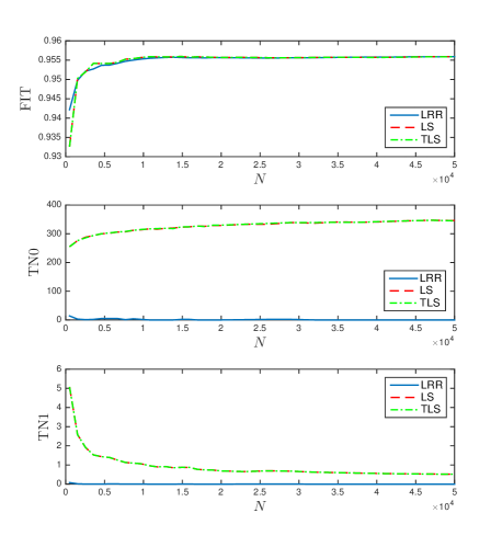
Figure 1: Values of FIT, TN0 and TN1 for all models.

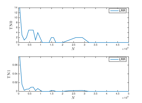
Figure 2: Values of TN0 and TN1 for the LRR models.

6.2 Experimental data from a flexible robot arm

The identification of poorly damped systems from experimental data is among the most challenging issues in many practical applications. For this reason, as second test we considered a system with a vibrating flexible robot arm described in Torfs et al. (1998), adopted as case study in various software packages (Kollár et al. (1994); Kollár (1994); National Instruments Corporation (2004-2006)). Data records from this process have been also analyzed in Pintelon and Schoukens (2012); Pillonetto et al. (2014). The input is the driving torque and the output is the tangential acceleration of the tip of the robot arm. Ten consecutive periods of the response to a multisine excitation signal were collected at a sampling frequency of 500 Hz, for a total of 40960 data points.

We have built models using different techniques: the Leading Response Recovery (LRR) and the regularized Diagonal/Correlated kernel (DCK) methods to obtain high-order FIR models, the standard Prediction Error Method (PEM) to estimate low-order state space models. Since the true system is unknown, the models cannot be evaluated by their fit to the actual system. Instead, we used the hold-out validation technique and measured how well the identified models can reproduce the output on validation portions of the data that were not used for estimation. We chose the estimation data to be the portion 1:7000 and the validation data to be the portion 10000:40960.

To identify the LRR models, the procedure described in Section 5 has been applied to suitably choose the values of $\sigma_{u}$ and $\gamma$, taking $q=7000$ as initial estimate length. No a-priori information was available about the input noise affecting the system, driven by an input signal $u$ with sample variance $\nu^{2}=0.0298$. For this reason, three scenarios have been considered, with $\sigma_{u}=0$, $\sigma_{u}=0.02$ and $\sigma_{u}=0.04$. These values correspond to noise-to-signal ratios of $0\%$ (i.e., no-input-noise situation), $1.3\%$, and $5.3\%$, respectively. Then the LRR algorithm has run with values of $\gamma$ in the range $\left[0.01,\ 1\right]$, using the MATLAB’s command lasso with optional input arguments ’RelTol’,4e-4,’Standardize’,false. The results in terms of fitting error $\left\|y-Ux^{*}\right\|_{2}^{2}$ and complexity $\left\|x^{*}\right\|_{0}$ are shown in Figure 3 (lower error and higher complexity are achieved for lower values of $\gamma$). As expected, curves with lower $\sigma_{u}$ dominate curves with higher $\sigma_{u}$ (for any given $\gamma$, the solution obtained with lower $\sigma_{u}$ has both lower error and complexity with respect to a solution obtained with higher $\sigma_{u}$). However, the choice of the actual curve to use depends on our confidence on the true value of $\sigma_{u}$, and underestimating this value may lead to worse-than-expected performance on validation data. Also, curves with higher $\sigma_{u}$ show a flatter behavior after the “knee” for lower $\gamma$ values.

We found a reasonable tradeoff for $\gamma=0.2$, allowing a satisfactory fitting error (around $19.8$ for $\sigma_{u}=0$, which raises up to $21.1$ in the worst-case $\sigma_{u}=0.04$) with a small complexity (around $560$, that raises up to $1220$ for $\sigma_{u}=0.04$). Alternatively, $\gamma=0.1$ allows a lower error (around $14.8$ for $\sigma_{u}=0$, which raises up to $16.1$ for $\sigma_{u}=0.04$) with a still acceptable complexity (around $830$, that raises up to $1740$ for $\sigma_{u}=0.04$).

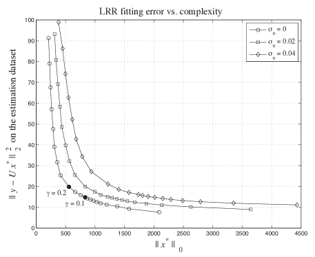
Figure 3: LRR fitting error $\left\|y-Ux^{*}\right\|_{2}^{2}$ vs. complexity $\left\|x^{*}\right\|_{0}$.

To fairly compare the performances achieved by LRR and DCK methods, FIR models with the same given order have been identified. First, the LRR FIR model of order $2500$ was identified with FIT value of 80.1%. Then, the DCK FIR model of order $2500$ was estimated using regularized least squares, tuned by the marginalized likelihood method and with the unknown input data set to zero, via the MATLAB’s command impulseest(data,2500,0,opt) with option opt set as opt.RegulKernel=’dc’; opt. Advanced.AROrder=0. The FIT for this DCK FIR model was 79.9%. For illustration, the FIT values of the LRR and DCK FIR models are shown in Figure 4 as horizontal lines. For comparison, we estimated $n$-th order state space PEM models without disturbance model for $n=1,\ldots,30$ (via the MATLAB’s command pem(data,n,’dist’,’no’)) and calculated their FIT index to validation data. These FIT values are shown as function of $n$ in Figure 4. The two best FITs were 78.9% and 78.6%, obtained for order $n=21$ and $n=18$, respectively, while the $5$-th order model with FIT value of 69.6% could be a reasonable tradeoff between accuracy and complexity. In any case, any PEM fit is worst than those provided by the LRR and DCK FIR models.

One may observe that FIR models of order $2500$ are quite large, but it is interesting to note that they can be easily reduced to low-order state space models by model order reduction methods, like balanced truncation, Hankel norm minimization and $\mathcal{L}_{2}$ reduction. For example, we applied the square root balanced truncation method to the LRR FIR model, to obtain reduced state space models of order $n=1,\ldots,30$ (via the MATLAB’s command balancmr), and we computed their FIT index on validation data. These FIT values are also shown as function of $n$ in Figure 4. It can be observed that a reduced state-space model of order $n=6$ provides a FIT of 74.2%, which is better than any PEM-estimated state space model of order $n=1,\ldots,14$.

To discriminate the effects of the transient due to the mismatch between the initial states of the actual system and the identified models, the FIT index has been also computed by neglecting the initial 3000 samples of the validation data. The FIT values of the LRR and DCK FIR models of order $2500$ raise to 83.4% and 83.6%, respectively; the FIT values of the PEM models of order $n=5,18,21$ go to 71.2%, 83.2%, 83.7%, respectively; the FIT value of the reduced state-space model of order $n=6$ increases to 76.2%. All these results are shown in Figure 5.

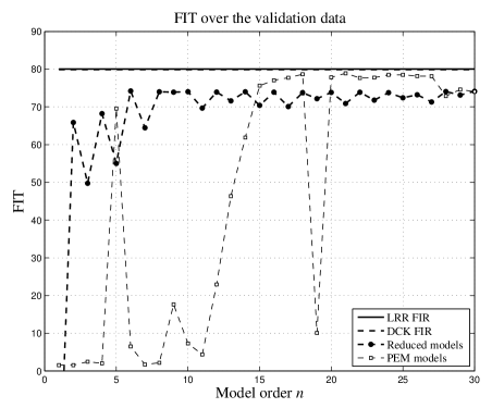
Figure 4: Values of FIT for all models.

Figure 5: Values of FIT, neglecting the starting 3000 samples.

It is worth to observe that, even if the fit performances of LRR and DCK FIR models are very close, the computational complexity of their corresponding algorithms is dramatically different. Referring to a workstation equipped with an Intel(R) Core(TM) i7-3770 CPU @ 3.40 GHz and with 16 GB of RAM, the overall CPU time used to estimate the LRR FIR model of order $2500$ was around $30$ seconds, while the computation of DCK FIR model of order $2500$ required around $8700$ seconds, i.e., $290$ times more. For comparison, FIR models of order $3000$ and $3500$ were also identified using the same 7000 estimation data as before: the CPU times required by the LRR FIR models were around $30$ and $36$ seconds, respectively, while the CPU times required by the DCK FIR models were around $11000$ and $23200$ seconds, respectively. Widening the estimation data to the first 10000 samples, the identification of LRR FIR models of orders up to 5000 required no more than $75$ seconds, thus showing that the approach proposed in this paper scales nicely with the problem dimensionality.

7 Conclusions

A novel method for the identification of low-complexity FIR models from experimental data is presented in this paper. The method is based on an Elastic Net criterion, which considers an identification cost defined as a weighted combination of a standard prediction error term, an $\ell_{2}$ regularization term, and a weighted $\ell_{1}$ penalty term. The main novelty of the method with respect to the state of the art is that it allows for an effective selection of the model order, while requiring only stability and standard statistical assumptions on the noises affecting the system; no additional information on the system impulse response behavior is needed. The effectiveness of the method has been tested through both extensive numerical simulations (considering two typical situations: one with a fixed number of data, and one with an arbitrarily large number of data) and real experimental data from a lightly damped mechanical system. In all situations, the method showed high numerical efficiency and satisfactory order selection capability and simulation accuracy.

Research activity is being devoted to developing a weighted version of the method proposed here. It is indeed expected that including suitable weights in the identification criterion may make the model order selection even more efficient, especially in situations where a low number of data is available.

Appendix A Appendix

A.1 Proof of Lemma 1

From the hypothesis that $y_{i}\leadsto\bar{y}_{i}$, $i=1,\ldots,p$, applying the definition of symbol $\leadsto$, we have that for any $\tilde{\epsilon}>0$ and $\tilde{\beta}\in(0,1)$ there exists an integer $\tilde{N}_{\tilde{\epsilon},\tilde{\beta}}$ such that

$$\mathbb{P}\{|y_{i}-\bar{y}_{i}|\leq\tilde{\epsilon}\}\geq 1-\tilde{\beta},\quad\forall N\geq\tilde{N}_{\tilde{\epsilon},\tilde{\beta}}.$$

From Bonferroni’s inequality we further have that the probability of the joint event $\{|y_{i}-\bar{y}_{i}|\leq\tilde{\epsilon},\,i=1,\ldots,p\}$ is lower bounded as

$$\mathbb{P}\{|y_{i}-\bar{y}_{i}|\leq\tilde{\epsilon},\,i=1,\ldots,p\}\geq 1-p\tilde{\beta},\quad\forall N\geq\tilde{N}_{\tilde{\epsilon},\tilde{\beta}}.$$

Since $\mathbb{P}\{|y_{i}-\bar{y}_{i}|\leq\tilde{\epsilon},\,i=1,\ldots,p\}=\mathbb{P}\{\|y-\bar{y}\|_{\infty}\leq\tilde{\epsilon}\}$, letting $\beta\doteq p\tilde{\beta}$, we write

$$\mathbb{P}\{\|y-\bar{y}\|_{\infty}\leq\tilde{\epsilon}\}\geq 1-\beta,\quad\forall N\geq\tilde{N}_{\tilde{\epsilon},\beta/p}.$$

Now, from the hypothesis that $f$ is Lipschitz continuous, it follows that there exists a finite constant $C\geq 0$ such that

$$|f(y)-f(\bar{y})|\leq C\|y-\bar{y}\|_{\infty}.$$

Therefore, $\|y-\bar{y}\|_{\infty}\leq\tilde{\epsilon}$ implies that $|f(y)-f(\bar{y})|\leq\epsilon$, for $\epsilon\doteq C\tilde{\epsilon}$, whence

$$\mathbb{P}\{|f(y)-f(\bar{y})|\leq\epsilon\}\geq 1-\beta,\quad\forall N\geq\tilde{N}_{\epsilon/C,\beta/p},$$

which proves that $f(y)\leadsto f(\bar{y})$.    

A.2 Proof of Lemma 2

The claim is a direct consequence of the first point of Theorem 8 in Tropp (2006), where the index set $\Lambda$ is $\{1,\ldots,n\}$, and $\mbox{ERC}(\Lambda)$ in Tropp (2006) coincides with $\Upsilon_{n}(A)$. The symbol $a_{\Lambda}$ used in Theorem 8 of Tropp (2006) corresponds to $P_{n}b$, that is the best $\ell_{2}$ approximation of $b$ using a linear combination of the first $n$ columns of $A$. These first $n$ columns have unit $\ell_{2}$ norm and are indeed linearly independent, as requested by the hypotheses of Theorem 8 in Tropp (2006), due to the specific structure of $A=\bar{A}T$, where $\bar{A}$, shown in (10), has a multiple of the identity matrix $I_{q}$ as a bottom block.    

A.3 Proof of Lemma 3

Some parts of this result might possibly be derived as a particular case of Theorem 2.3 in Ljung (1999a); we here report a full proof for the specific case of interest in the present work. For $i=1,2,\ldots,$ let us define $u_{i}=\left[u(2\!-\!i)\;u(3\!-\!i)\;\cdots\;u(N\!+\!1\!-\!i)\right]^{\top}\!\in{{\mathbb{R}}^{N}}$. Then, for all $i$ and $j$, we have that

$$\begin{array}[]{ll}\frac{1}{N}u_{i}^{\top}\!u_{j}&=\frac{1}{N}\left[u(2\!-\!i)\,u(3\!-\!i)\cdots u(N\!+\!1\!-\!i)\right]\cdot\\ &\hskip 19.91692pt\left[u(2\!-\!j)\,u(3\!-\!j)\cdots u(N\!+\!1\!-\!j)\right]^{\top}\\ &=\frac{1}{N}\sum_{k=2}^{N+1}u(k-i)u(k-j)\\ &=\frac{1}{N}\sum_{k=1}^{N}u(k+1-i)u(k+1-j).\end{array}$$

Consider first the case where $i=j$. Then

$$\tfrac{1}{N}u_{i}^{\top}u_{i}=\tfrac{1}{N}\mathop{\textstyle\sum}\nolimits_{k=1}^{N}u(k+1-i)^{2}$$

is the empirical mean of the elements of the sequence of length $N$ of random variables $x_{k}=u(k\!+\!1\!-\!i)^{2}$, $k=1,\ldots,N$, such that, for all $k$, $i$ and $l\neq k$:

$$\mathbb{E}\{x_{k}\}=\mathbb{E}\{u(k\!+\!1\!-\!i)^{2}\}={\mathrm{var}}\{u(k\!+\!1\!-\!i)\}=\nu^{2}<\infty$$

$$\hskip 5.69054pt{\mathrm{var}}\{x_{k}\} = \mathbb{E}\left\{\left(x_{k}-\mathbb{E}\left\{x_{k}\right\}\right)^{2}\right\}=\mathbb{E}\left\{\left(u(k\!+\!1\!-\!i)^{2}\!-\!\nu^{2}\right)^{2}\right\}$$

$$= \mathbb{E}\left\{u(k\!+\!1\!-\!i)^{4}\!-\!2\nu^{2}u(k\!+\!1\!-\!i)^{2}\!+\!\nu^{4}\right\}$$

$$= \mathbb{E}\left\{u(k\!+\!1\!-\!i)^{4}\right\}-2\nu^{2}\mathbb{E}\left\{u(k\!+\!1\!-\!i)^{2}\right\}+\nu^{4}$$

$$= \overline{m\rule{0.0pt}{5.69054pt}_{4}}-\nu^{4}<\infty$$

$$\begin{array}[]{l}\mathbb{E}\left\{\left(x_{k}\!-\!\mathbb{E}\left\{x_{k}\right\}\right)\left(x_{l}\!-\!\mathbb{E}\left\{x_{l}\right\}\right)\right\}\\ \hskip 5.69054pt=\mathbb{E}\left\{\left(u(k\!+\!1\!-\!i)^{2}\!-\!\nu^{2}\right)\left(u(l\!+\!1\!-\!i)^{2}\!-\!\nu^{2}\right)\right\}\\ \hskip 5.69054pt=\mathbb{E}\left\{u(k\!+\!1\!-\!i)^{2}u(l\!+\!1\!-\!i)^{2}+\right.\\ \hskip 5.69054pt\hskip 22.76219pt\left.-\nu^{2}\!\left[u(k\!+\!1\!-\!i)^{2}\!+\!u(l\!+\!1\!-\!i)^{2}\right]\!+\!\nu^{4}\right\}\\ \hskip 5.69054pt=\mathbb{E}\left\{u(k\!+\!1\!-\!i)^{2}u(l\!+\!1\!-\!i)^{2}\right\}+\\ \hskip 5.69054pt\hskip 8.53581pt-\nu^{2}\!\left[\mathbb{E}\left\{u(k\!+\!1\!-\!i)^{2}\right\}\!+\!\mathbb{E}\left\{u(l\!+\!1\!-\!i)^{2}\right\}\right]\!+\!\nu^{4}\\ \hskip 5.69054pt=\mathbb{E}\left\{u(k\!+\!1\!-\!i)^{2}\right\}\mathbb{E}\left\{u(l\!+\!1\!-\!i)^{2}\right\}\!-\!\nu^{4}=\nu^{2}\nu^{2}-\nu^{4}=0\end{array}$$

where the last derivation follows from the fact that $x_{k}$ and $x_{l}$ are mutually independent since the input $u(k)$ is an i.i.d. sequence. By applying the Chebyshev’s inequality for sums of uncorrelated variables shown in Section 2.2, it holds that

$$\tfrac{1}{N}u_{i}^{\top}u_{i}\leadsto\mathbb{E}\{x_{k}\}=\nu^{2},\quad\forall i.$$

Consider next the case where $i\neq j$. Then

$$\tfrac{1}{N}u_{i}^{\top}\!u_{j}=\tfrac{1}{N}\mathop{\textstyle\sum}\nolimits_{k=1}^{N}u(k+1-i)u(k+1-j)$$

is the empirical mean of the elements of the sequence of length $N$ of random variables $x_{k}=u(k+1-i)u(k+1-j)$, $k=1,\ldots,N$, such that, for all $k$, $i$, $j=i+\tilde{i}\neq i$ and $l=k+\tilde{k}\neq k$, with $\tilde{i}\neq 0$ and $\tilde{k}\neq 0\,$:

$$\hskip 28.45274pt\mathbb{E}\{x_{k}\} = \mathbb{E}\left\{u(k\!+\!1\!-\!i)u(k\!+\!1\!-\!j)\right\}$$

$$= \mathbb{E}\left\{u(k\!+\!1\!-\!i)\right\}\mathbb{E}\left\{u(k\!+\!1\!-\!j)\right\}=0$$

$${\mathrm{var}}\{x_{k}\} = \mathbb{E}\!\left\{\!\left(x_{k}\!-\mathbb{E}\!\left\{x_{k}\right\}\right)^{2}\right\}\!=\!\mathbb{E}\!\left\{\!\left(u(k\!+\!1\!-\!i)u(k\!+\!1\!-\!j)\right)^{2}\right\}$$

$$= \mathbb{E}\!\left\{u(k\!+\!1\!-\!i)^{2}u(k\!+\!1\!-\!j)^{2}\right\}$$

$$= \mathbb{E}\!\left\{u(k\!+\!1\!-\!i)^{2}\right\}\mathbb{E}\!\left\{u(k\!+\!1\!-\!j)^{2}\right\}=\nu^{4}<\infty$$

$$\mathbb{E}\!\left\{\left(x_{k}\!-\!\mathbb{E}\!\left\{x_{k}\right\}\right)\left(x_{l}\!-\!\mathbb{E}\!\left\{x_{l}\right\}\right)\right\}\!=$$

$$= \!\mathbb{E}\!\left\{\left(u(k\!+\!1\!-\!i)u(k\!+\!1\!-\!j)\right)\left(u(l\!+\!1\!-\!i)u(l\!+\!1\!-\!j)\right)\right\}$$

$$= \!\mathbb{E}\{u(k\!+\!1\!-\!i)u(k\!+\!1\!-\!i\!-\!\tilde{i})u(k\!+\!\tilde{k}\!+\!1\!-\!i)u(k\!+\!\tilde{k}\!+\!1\!-\!i\!-\!\tilde{i})\}$$

$$= \!\mathbb{E}\{u(k\!+\!1\!-\!i)u(k\!+\!1\!-\!i\!-\!\tilde{i})u(k\!+\!1\!-\!i\!+\!\tilde{k})u(k\!+\!1\!-\!i\!-\!\tilde{i}\!+\!\tilde{k})\}$$

if $\tilde{i}=\tilde{k}$, then:

$$\mathbb{E}\left\{\left(x_{k}\!-\!\mathbb{E}\left\{x_{k}\right\}\right)\left(x_{l}\!-\!\mathbb{E}\left\{x_{l}\right\}\right)\right\}=$$

$$= \mathbb{E}\left\{u(k\!+\!1\!-\!i)^{2}u(k\!+\!1\!-\!i\!-\!\tilde{i})u(k\!+\!1\!-\!i\!+\!\tilde{i})\right\}$$

$$= \mathbb{E}\left\{u(k\!+\!1\!-\!i)^{2}\right\}\mathbb{E}\left\{u(k\!+\!1\!-\!i\!-\!\tilde{i})\right\}\mathbb{E}\left\{u(k\!+\!1\!-\!i\!+\!\tilde{i})\right\}=0$$

otherwise, if $\tilde{i}\neq\tilde{k}$, then:

$$\mathbb{E}\left\{\left(x_{k}\!-\!\mathbb{E}\left\{x_{k}\right\}\right)\left(x_{l}\!-\!\mathbb{E}\left\{x_{l}\right\}\right)\right\}=$$

$$= \mathbb{E}\{u(k\!+\!1\!-\!i)u(k\!+\!1\!-\!i\!-\!\tilde{i})u(k\!+\!1\!-\!i\!+\!\tilde{k})u(k\!+\!1\!-\!i\!-\!\tilde{i}\!+\!\tilde{k})\}$$

$$= \mathbb{E}\!\left\{u(k\!+\!1\!-\!i)\right\}\cdot$$

$$\mathbb{E}\{u(k\!+\!1\!-\!i\!-\!\tilde{i})u(k\!+\!1\!-\!i\!+\!\tilde{k})u(k\!+\!1\!-\!i\!-\!\tilde{i}\!+\!\tilde{k})\}\mbox{\thinspace=\thinspace 0}$$

and this means that $x_{k}$ and $x_{l}$ are uncorrelated for all $k\neq l$. By applying the Chebyshev’s inequality for sums of uncorrelated variables shown in Section 2.2, we obtain that

$$\tfrac{1}{N}u_{i}^{\top}u_{j}\leadsto\mathbb{E}\{x_{k}\}=0\text{, for all }i\neq j,$$

which proves (16).

We next prove (17). Since $\delta_{y}\!=\!\left[\delta_{y}(1)\,\delta_{y}(2)\,\cdots\,\delta_{y}(N)\right]^{\top}\!\!\in\!{{\mathbb{R}}^{N}\!}$, then for $i=1,2,\ldots$:

$$\hskip 28.45274pt\tfrac{1}{N}u_{i}^{\top}\!\delta_{y} = \tfrac{1}{N}\left[u(2\!-\!i)\,u(3\!-\!i)\cdots u(N\!+\!1\!-\!i)\right]\cdot$$

$$\hskip 10.243pt\left[\delta_{y}(1)\;\delta_{y}(2)\;\cdots\;\delta_{y}(N)\right]^{\top}$$

$$= \tfrac{1}{N}\mathop{\textstyle\sum}\nolimits_{k=1}^{N}u(k+1-i)\delta_{y}(k)$$

is the empirical mean of the elements of the sequence of length $N$ of random variables $x_{k}=u(k+1-i)\delta_{y}(k)$, $k=1,\ldots,N$, such that, for all $k$, $i$ and $l\neq k$:

$$\mathbb{E}\{x_{k}\}\!=\!\mathbb{E}\{u(k+1-i)\delta_{y}(k)\}\!=\!\mathbb{E}\{u(k+1-i)\}\mathbb{E}\{\delta_{y}(k)\}\!=\!0$$

$$\hskip 5.69054pt{\mathrm{var}}\{x_{k}\}\! = \!\mathbb{E}\left\{\left(x_{k}-\mathbb{E}\left\{x_{k}\right\}\right)^{2}\right\}$$

$$= \!\mathbb{E}\left\{\left(u(k\!+\!1\!-\!i)\delta_{y}(k)\right)^{2}\right\}\!=\!\mathbb{E}\left\{u(k\!+\!1\!-\!i)^{2}\delta_{y}(k)^{2}\right\}$$

$$= \!\mathbb{E}\left\{u(k\!+\!1\!-\!i)^{2}\right\}\mathbb{E}\left\{\delta_{y}(k)^{2}\right\}=\nu^{2}\sigma_{y}^{2}<\infty$$

$$\mathbb{E}\left\{\left(x_{k}\!-\!\mathbb{E}\left\{x_{k}\right\}\right)\left(x_{l}\!-\!\mathbb{E}\left\{x_{l}\right\}\right)\right\}=$$

$$= \mathbb{E}\left\{\left(u(k\!+\!1\!-\!i)\delta_{y}(k)\right)\left(u(l\!+\!1\!-\!i)\delta_{y}(l)\right)\right\}$$

$$= \mathbb{E}\left\{u(k\!+\!1\!-\!i)u(l\!+\!1\!-\!i)\delta_{y}(k)\delta_{y}(l)\right\}$$

$$= \mathbb{E}\left\{u(k\!+\!1\!-\!i)\right\}\mathbb{E}\left\{u(l\!+\!1\!-\!i)\right\}\mathbb{E}\left\{\delta_{y}(k)\right\}\mathbb{E}\left\{\delta_{y}(l)\right\}=0\text{.}$$

By applying the Chebyshev’s inequality for sums of uncorrelated variables shown in Section 2.2, it thus holds that

$$\tfrac{1}{N}u_{i}^{\top}\delta_{y}\leadsto\mathbb{E}\{x_{k}\}=0\text{, for all }i\text{.}$$

Finally, we prove (18). For $j=1,2,\ldots,$ let us define $\delta_{j}=\left[\delta_{u}(2\!-\!j)\;\delta_{u}(3\!-\!j)\;\cdots\;\delta_{u}(N\!+\!1\!-\!j)\right]^{\top}\!\in{{\mathbb{R}}^{N}}$. Then, $\forall i,j$:

$$\hskip 22.76219pt\tfrac{1}{N}u_{i}^{\top}\!\delta_{j} = \tfrac{1}{N}\left[u(2\!-\!i)\,u(3\!-\!i)\cdots u(N\!+\!1\!-\!i)\right]\cdot$$

$$\hskip 10.243pt\left[\delta_{u}(2\!-\!j)\,\delta_{u}(3\!-\!j)\cdots\delta_{u}(N\!+\!1\!-\!j)\right]^{\top}$$

$$= \tfrac{1}{N}\mathop{\textstyle\sum}\nolimits_{k=2}^{N+1}u(k-i)\delta_{u}(k-j)$$

$$= \tfrac{1}{N}\mathop{\textstyle\sum}\nolimits_{k=1}^{N}u(k+1-i)\delta_{u}(k+1-j)$$

is the empirical mean of the elements of the sequence of length $N$ of random variables $x_{k}=u(k+1-i)\delta_{u}(k+1-j)$, $k=1,\ldots,N$, such that, for all $k$, $i$, $j$ and $l\neq k$:

$$\hskip 22.76219pt\mathbb{E}\{x_{k}\} = \mathbb{E}\left\{u(k\!+\!1\!-\!i)\delta_{u}(k\!+\!1\!-\!j)\right\}$$

$$= \mathbb{E}\left\{u(k\!+\!1\!-\!i)\right\}\mathbb{E}\left\{\delta_{u}(k\!+\!1\!-\!j)\right\}=0$$

$${\mathrm{var}}\{x_{k}\}\! = \!\mathbb{E}\!\left\{\left(x_{k}\!-\mathbb{E}\!\left\{x_{k}\right\}\right)^{2}\right\}\!=\!\mathbb{E}\!\left\{\!\left(u(k\!+\!1\!-\!i)\delta_{u}(k\!+\!1\!-\!j)\right)^{2}\right\}$$

$$= \!\mathbb{E}\!\left\{u(k\!+\!1\!-\!i)^{2}\delta_{u}(k\!+\!1\!-\!j)^{2}\right\}\!$$

$$= \!\mathbb{E}\!\left\{u(k\!+\!1\!-\!i)^{2}\right\}\mathbb{E}\!\left\{\delta_{u}(k\!+\!1\!-\!j)^{2}\right\}=\nu^{2}\sigma_{u}^{2}<\infty$$

$$\mathbb{E}\left\{\left(x_{k}\!-\!\mathbb{E}\left\{x_{k}\right\}\right)\left(x_{l}\!-\!\mathbb{E}\left\{x_{l}\right\}\right)\right\}=$$

$$= \mathbb{E}\left\{\left(u(k\!+\!1\!-\!i)\delta_{u}(k\!+\!1\!-\!j)\right)\left(u(l\!+\!1\!-\!i)\delta_{u}(l\!+\!1\!-\!j)\right)\right\}$$

$$= \mathbb{E}\left\{u(k\!+\!1\!-\!i)u(l\!+\!1\!-\!i)\delta_{u}(k\!+\!1\!-\!j)\delta_{u}(l\!+\!1\!-\!j)\right\}$$

$$= \mathbb{E}\left\{u(k\!+\!1\!-\!i)\right\}\mathbb{E}\left\{u(l\!+\!1\!-\!i)\right\}\cdot$$

$$\hskip 8.53581pt\mathbb{E}\left\{\delta_{u}(k\!+\!1\!-\!j)\right\}\mathbb{E}\left\{\delta_{u}(l\!+\!1\!-\!j)\right\}\mbox{$=0\text{.}$}$$

By applying the Chebyshev’s inequality for sums of uncorrelated variables shown in Section 2.2, it holds that

$$\tfrac{1}{N}u_{i}^{\top}\delta_{j}\leadsto\mathbb{E}\{x_{k}\}=0\text{, for all }i\text{ and }j\text{.}$$

   

A.4 Proof of Theorem 4

A.4.1 Preliminaries

For any integer $n\leq q$, let $h^{n}\doteq[h(1)\,\cdots\,h(n)\,0\,\cdots\,0]^{\top}\in{\ {\mathbb{R}}^{q}}$ denote the $n$-leading truncation of $h_{\uparrow q}\in{\ {\mathbb{R}}^{q}}$, let

$$h_{\downarrow n}=[h(n+1)\,h(n+2)\,\cdots]^{\top},$$

and let, for $i=1,2,\ldots,$

$$\tilde{u}_{i}\!\doteq\!\!\left[\!\!\begin{array}[]{c}\tilde{u}(2-i)\vspace*{-1.0mm}\\ \tilde{u}(3-i)\vspace*{-2.0mm}\\ \vdots\vspace*{-1.5mm}\\ \tilde{u}(N\!+\!1-i)\end{array}\!\!\right]\!\!,\,u_{i}\!\doteq\!\!\left[\!\!\begin{array}[]{c}u(2-i)\vspace*{-1.0mm}\\ u(3-i)\vspace*{-2.0mm}\\ \vdots\vspace*{-1.5mm}\\ u(N\!+\!1-i)\end{array}\!\!\right]\!\!,\,\delta_{i}\!\doteq\!\!\left[\!\!\begin{array}[]{c}\delta_{u}(2-i)\vspace*{-1.0mm}\\ \delta_{u}(3-i)\vspace*{-2.0mm}\\ \vdots\vspace*{-1.5mm}\\ \delta_{u}(N\!+\!1-i)\end{array}\!\!\right]\!\!.$$

For any integer $k\geq 1$, let $\Delta_{\uparrow k}\doteq[\delta_{1}\,\cdots\,\delta_{k}]$, $\Delta_{\downarrow k}\doteq[\delta_{k+1}\,\cdots]$ and define $\Delta_{\downarrow 0}=[\delta_{1}\,\delta_{2}\,\cdots]\in{{\mathbb{R}}^{N,\infty}}$. Considering the expression in (4), and splitting the summation at $n$, we can write

$$y=\tilde{U}_{\uparrow n}h_{\uparrow n}+\delta_{y}+\tilde{U}_{\downarrow n}h_{\downarrow n}.$$

Further, using (6), we have

$$y=U_{\uparrow n}h_{\uparrow n}+(\Delta_{\uparrow n}h_{\uparrow n}+\delta_{y}+U_{\downarrow n}h_{\downarrow n}+\Delta_{\downarrow n}h_{\downarrow n}).$$

Since $U_{\uparrow n}h_{\uparrow n}=U_{\uparrow q}h^{n}\doteq Uh^{n}$, we can write

$$y=Uh^{n}+e_{0},$$

where

$$e_{0}\doteq U_{\downarrow n}h_{\downarrow n}+\Delta_{\downarrow 0}h+\delta_{y},$$

being $h\doteq[h(1)\,h(2)\,\cdots]^{\top}$. Then, using the notation in (10), we have that

$$b=\bar{A}h^{n}+e,$$

where

$$e\doteq\left[\begin{array}[]{c}\vspace*{-7.0mm}\hfil\\ e_{0}\vspace*{-1.0mm}\\ -\sigma_{u}\sqrt{N}h^{n}\end{array}\right],$$ (23)

and, by the change of variable $\tilde{h}^{n}=T^{-1}h^{n}$,

$$b=A\tilde{h}^{n}+e.$$

Since $A=\bar{A}T$, where $T$ is diagonal, we can write

$$A_{\uparrow n}=\bar{A}_{\uparrow n}T_{\sharp n},$$

where $T_{\sharp n}$ is the $n\times n$ principal submatrix of $T$. Therefore,

$$\hskip 14.22636ptA_{\uparrow n}^{\dagger} = (A_{\uparrow n}^{\top}A_{\uparrow n})^{-1}A_{\uparrow n}^{\top}=T_{\sharp n}^{-1}\bar{A}_{\uparrow n}^{\dagger}$$

$$= T_{\sharp n}^{-1}\left(U_{\uparrow n}^{\top}U_{\uparrow n}+N\sigma_{u}^{2}I_{n}\right)^{-1}\left[\begin{array}[]{cc}U_{\uparrow n}^{\top}&\sigma_{u}\sqrt{N}I_{\uparrow n}^{\top}\end{array}\right],$$

where $I_{\uparrow n}$ is the submatrix formed by the first $n$ columns of the identity matrix $I_{q}$.

The orthogonal projector $P_{n}$ onto the span of $A_{\uparrow n}$ is given by

$$P_{n} = A_{\uparrow n}A_{\uparrow n}^{\dagger}=\bar{A}_{\uparrow n}\bar{A}_{\uparrow n}^{\dagger}$$

$$= \left[\!\begin{array}[]{c}\vspace*{-7.0mm}\hfil\\ U_{\uparrow n}\vspace*{-1.0mm}\\ \sigma_{u}\sqrt{N}I_{\uparrow n}\end{array}\!\right]\!\left(U_{\uparrow n}^{\top}U_{\uparrow n}\!+\!N\sigma_{u}^{2}I_{n}\right)^{-1}\!\left[\!\begin{array}[]{cc}U_{\uparrow n}^{\top}&\sigma_{u}\sqrt{N}I_{\uparrow n}^{\top}\end{array}\!\right].$$

For any given vector $b$, the best $\ell_{2}$ approximation of $b$ using the columns in $A_{\uparrow n}$ is given by $b_{n}=P_{n}b$, where, by the Projection theorem, $b_{n}\bot(b-b_{n})$. The corresponding optimal coefficient vector is $x_{n}=A_{\uparrow n}^{\dagger}b=A_{\uparrow n}^{\dagger}b_{n}$.

For a column $a_{i}$ of $A$, $i=1,\ldots,q$, we have that

$$A_{\uparrow n}^{\dagger}a_{i} = t_{i}A_{\uparrow n}^{\dagger}\bar{a}_{i}$$

$$= t_{i}T_{\sharp n}^{-1}(U_{\uparrow n}^{\top}U_{\uparrow n}/N\!+\sigma_{u}^{2}I_{n})^{-1}(U_{\uparrow n}^{\top}u_{i}/N\!+\sigma_{u}^{2}I_{\uparrow n}^{\top}\zeta_{i}),$$

where $\zeta_{i}$ is the $i$-th column of the identity matrix $I_{q}$, and $t_{i}\doteq[T]_{i,i}=\|\bar{a}_{i}\|_{2}^{-1}=\left(u_{i}^{\top}u_{i}+N\sigma_{u}^{2}\right)^{-1/2}$.

We shall next examine the condition in (15).

A.4.2 The large $N$ sparsity pattern

From Lemma 3, we have that $U_{\uparrow n}^{\top}U_{\uparrow n}/N\!\leadsto\!\nu^{2}I_{n}$, and $U_{\uparrow n}^{\top}u_{i}/N\!\leadsto 0_{n,1}$, if $i>n$. Moreover, $t_{i}T_{\sharp n}^{-1}\leadsto I_{n}$, and $I_{\uparrow n}^{\top}\zeta_{i}\!=\!\left[\!\begin{array}[]{cc}I_{n}&0_{n,q-n}\end{array}\!\right]\zeta_{i}=0_{n,1}$, if $i>n$. Therefore, considering the scalar-valued function $\|W_{\sharp n}A_{\uparrow n}^{\dagger}a_{i}\|_{1}$, which is Lipschitz continuous w.r.t. the entries of $U_{\uparrow n}^{\top}U_{\uparrow n}/N$ and $U_{\uparrow n}^{\top}u_{i}/N$, and applying Lemma 1, we obtain that, for $i>n$,

$$\begin{array}[]{l}\left\|W_{\sharp n}A_{\uparrow n}^{\dagger}a_{i}\right\|_{1}\rule[-8.53581pt]{0.0pt}{8.53581pt}\leadsto\\ \left\|W_{\sharp n}t_{i}T_{\sharp n}^{-1}\tfrac{\sigma_{u}^{2}}{\nu^{2}+\sigma_{u}^{2}}I_{\uparrow n}^{\top}\zeta_{i}\right\|_{1}=\left\|W_{\sharp n}I_{n}\tfrac{\sigma_{u}^{2}}{\nu^{2}+\sigma_{u}^{2}}0_{n,1}\right\|_{1}=0.\vspace*{0em}\end{array}$$

Hence it holds that

$$\Upsilon_{n}(A)=1-\max_{i>n}w_{i}^{-1}\left\|W_{\sharp n}A_{\uparrow n}^{\dagger}a_{i}\right\|_{1}\leadsto 1-0=1.$$ (26)

Let us now consider the left-hand side in the condition (15). Using the fact that $b=\bar{A}h^{n}+e$, with $e$ given in (23), we have

$$\begin{array}[]{l}W^{-1}A^{\top}(b-\!P_{n}b)=W^{-1}T\bar{A}^{\top}(\bar{A}h^{n}+e-\!P_{n}\bar{A}h^{n}\!-\!P_{n}e)\text{{}}\\ =W^{-1}T(\bar{A}^{\top}\!\bar{A}h^{n}\!+\bar{A}^{\top}e-\bar{A}^{\top}\!P_{n}\bar{A}h^{n}\!-\bar{A}^{\top}\!P_{n}e).\vspace*{-1.3em}\end{array}$$ (27)

Defining $\tilde{T}\doteq T\sqrt{N}$ and dividing (27) by $\sqrt{N}$, we obtain

$$\begin{array}[]{l}\frac{1}{\sqrt{N}}W^{-1}A^{\top}(b-P_{n}b)=\\ =W^{-1}\tilde{T}(\bar{A}^{\top}\!\bar{A}h^{n}\!+\!\bar{A}^{\top}\!e-\!\bar{A}^{\top}\!P_{n}\bar{A}h^{n}\!-\!\bar{A}^{\top}\!P_{n}e)\left/N\right.\!.\vspace*{1.8em}\end{array}$$ (28)

Now we evaluate

$$\hskip 11.38109pt\bar{A}^{\top}\!\bar{A}/\!N\! = U^{\top}\!U/\!N+\sigma_{u}^{2}I_{q}$$

$$\bar{A}^{\top}\!e/\!N\! = U^{\top}\!U_{\downarrow n}h_{\downarrow n}/\!N\!+U^{\top}\!\Delta_{\downarrow 0}h/\!N\!+U^{\top}\!\delta_{y}/\!N\!-\!\sigma_{u}^{2}h^{n}$$

$$\bar{A}^{\top}\!\!P_{n}\bar{A}h^{n}\!/\!N\! = (U^{\top}\!U/\!N+\sigma_{u}^{2}I_{q})h^{n}$$

$$\bar{A}^{\top}\!\!P_{n}e/\!N\! = (U^{\top}\!U_{\uparrow n}/\!N+\sigma_{u}^{2}I_{\uparrow n})(U_{\uparrow n}^{\top}U_{\uparrow n}/\!N+\sigma_{u}^{2}I_{n})^{-1}\cdot$$

$$\{[U_{\uparrow n}^{\top}U_{\downarrow n}h_{\downarrow n}\!\!+\!U_{\uparrow n}^{\top}(\Delta_{\downarrow 0}h\!+\!\delta_{y})]/\!N\!-\!\sigma_{u}^{2}I_{\uparrow n}^{\top}h^{n}\}$$

and observe that

$$\hskip 71.13188ptU^{\top}U/N \leadsto \nu^{2}I_{q}$$

$$U^{\top}U_{\downarrow n}h_{\downarrow n}/N \leadsto \nu^{2}(h^{q}-h^{n})$$

$$U^{\top}U_{\uparrow n}/N \leadsto \left[\begin{array}[]{c}\vspace*{-6.0mm}\hfil\\ \nu^{2}I_{n}\vspace*{-1.0mm}\\ 0\vspace*{-1.0mm}\end{array}\right]$$

$$U^{\top}\Delta_{\downarrow 0}h/N \leadsto 0$$

$$\hskip 71.13188ptU^{\top}\delta_{y}/N \leadsto 0$$

$$U_{\uparrow n}^{\top}U_{\downarrow n}h_{\downarrow n}/N \leadsto 0$$

hence

$$\hskip 71.13188pt\bar{A}^{\top}\bar{A}/N \leadsto (\nu^{2}+\sigma_{u}^{2})I_{q}$$

$$\bar{A}^{\top}e/N \leadsto \nu^{2}(h^{q}-h^{n})-\sigma_{u}^{2}h^{n}$$

$$\bar{A}^{\top}P_{n}\bar{A}h^{n}/N \leadsto (\nu^{2}+\sigma_{u}^{2})h^{n}$$

$$\bar{A}^{\top}P_{n}e/N \leadsto -\sigma_{u}^{2}h^{n}.$$

Substituting in (28) we obtain that

$$\tfrac{1}{\sqrt{N}}W^{-1}A^{\top}(b-P_{n}b)\leadsto{\nu^{2}}W^{-1}\tilde{T}(h^{q}-h^{n}).$$ (30)

Finally, observe that for the $i$-th diagonal element $t_{i}$ of $T$ it holds that (by Lemma 1)

$$t_{i}^{2}=\frac{1}{\|\bar{a}_{i}\|_{2}^{2}}=\frac{1}{\|u_{i}\|_{2}^{2}+\sigma_{u}^{2}N}\leadsto\frac{1}{N(\nu^{2}+\sigma_{u}^{2})}$$

and thus, for the $i$-th diagonal element $\tilde{t}_{i}$ of $\tilde{T}$, we have

$$\tilde{t}_{i}^{2}\leadsto\frac{1}{\nu^{2}+\sigma_{u}^{2}}.$$

Therefore, from (30), we obtain that

$$\frac{1}{\sqrt{N}}[W^{-1}\!A^{\top}\!(b-\!P_{n}b)]_{i}\leadsto z_{i}\!\doteq\!\left\{\!\begin{array}[]{l}\vspace*{-6.0mm}\\ 0,\hskip 8.53581pt\mbox{for }i=1,\ldots,n;\\ w_{i}^{-1}\nu\kappa h(i),\\ \hskip 17.07164pt\mbox{for }i=n+1,\ldots,q.\vspace*{-1.0mm}\end{array}\right.$$

where $\kappa\doteq\nu/\sqrt{\nu^{2}+\sigma_{u}^{2}}$.

From the definition of the symbol $\leadsto$, the above expression implies that for any given $\epsilon_{1}>0$ and $\beta_{1}\in(0,1)$ there exists an integer $N_{1}$ such that, for any $N\!\geq\!N_{1}$, it results

$$\mathbb{P}\left\{\left|\tfrac{1}{\sqrt{N}}|[W^{-1}A^{\top}\!(b-\!P_{n}b)]_{i}|\!-\!|z_{i}|\right|\geq\epsilon_{1}\!\right\}\leq\beta_{1}.$$ (31)

Further, under the Assumption 2 that $|h(i)|\leq L\rho^{i-1}$ and since the weight sequence is assumed to be nondecreasing, we have that

$$\hskip 19.91692pt|z_{i}|\leq w_{n}^{-1}\nu\kappa L\rho^{n},\quad\forall i=1,\ldots,q.$$ (32)

Since, for all $i=1,\ldots,q$,

$$\begin{array}[]{l}\left|\frac{1}{\sqrt{N}}|[W^{-1}A^{\top}(b-P_{n}b)]_{i}|-|z_{i}|\right|\geq\\ \hskip 14.22636pt\geq\tfrac{1}{\sqrt{N}}|[W^{-1}A^{\top}(b-P_{n}b)]_{i}|-|z_{i}|\\ \hskip 14.22636pt\geq\tfrac{1}{\sqrt{N}}|[W^{-1}A^{\top}(b-P_{n}b)]_{i}|-w_{n}^{-1}\nu\kappa L\rho^{n},\end{array}$$

from (31) it follows that, for any $N\!\geq\!N_{1}$,

$$\mathbb{P}\!\left\{\!\tfrac{1}{\sqrt{N}}|[W^{-1}A^{\top}\!(b-\!P_{n}b)]_{i}|-w_{n}^{-1}\nu\kappa L\rho^{n}\geq\epsilon_{1}\!\right\}\leq\beta_{1};$$

hence, from Bonferroni’s inequality, for any $N\!\geq\!N_{1}$ we have

$$\mathbb{P}\!\left\{\!\tfrac{1}{\sqrt{N}}\|W^{-1}A^{\top}\!(b-\!P_{n}b)\|_{\infty}\!>w_{n}^{-1}\nu\kappa L\rho^{n}\!\!+\!\epsilon_{1}\!\right\}\!\leq\!q\beta_{1}.$$

Taking the complementary event, for any $N\geq N_{1}$ it results

$$\mathbb{P}\!\left\{\!\tfrac{1}{\sqrt{N}}\|W^{-1}A^{\top}\!(b-\!P_{n}b)\|_{\infty}\!\leq\!w_{n}^{-1}\nu\kappa L\rho^{n}\!\!+\!\epsilon_{1}\!\right\}\!\geq\!1-q\beta_{1}.$$ (33)

Similarly, from (26) it follows that for any given $\epsilon_{2}>0$ and $\beta_{2}\in(0,1)$ there exists an integer $N_{2}$ such that

$$\mathbb{P}\{|\Upsilon_{n}(A)\!-\!1|\!\leq\!\epsilon_{2}\}\!=\!\mathbb{P}\{1\!-\!\Upsilon_{n}(A)\!\leq\!\epsilon_{2}\}\!\geq\!1\!-\!\beta_{2},\;\forall N\!\geq\!N_{2};$$ (34)

thus

$$\mathbb{P}\left\{\!\tfrac{\gamma}{2\sqrt{N}}\left(1\!-\!\epsilon_{2}\right)\leq\tfrac{\gamma}{2\sqrt{N}}\Upsilon_{n}\!(A)\!\right\}\geq 1\!-\!\beta_{2},\;\forall N\!\geq\!N_{2}.$$ (35)

Considering the joint events in (33) and (35), we have from Bonferroni’s inequality that

$$\hskip 8.53581pt\left\{\tfrac{1}{\sqrt{N}}\|W^{-1}A^{\top}\!(b-\!P_{n}b)\|_{\infty}\leq w_{n}^{-1}\nu\kappa L\rho^{n}+\epsilon_{1}\right\}\;\cap$$

$$\;\hskip 48.36967pt\left\{\tfrac{\gamma}{2\sqrt{N}}\left(1-\epsilon_{2}\right)\leq\tfrac{\gamma}{2\sqrt{N}}\Upsilon_{n}(A)\right\}$$

holds with probability no smaller than $1-\beta$, for any $N\geq N_{\beta}\doteq\max(N_{1},N_{2})$, with $\beta\doteq q\beta_{1}+\beta_{2}$. Next, observe that if it holds that

$$w_{n}^{-1}\nu\kappa L\rho^{n}+\epsilon_{1}\leq\tfrac{\gamma}{2\sqrt{N}}\left(1-\epsilon_{2}\right),$$ (36)

then we may conclude with confidence at least $1-\beta$ that

$$\tfrac{1}{\sqrt{N}}\|W^{-1}A^{\top}(b-P_{n}b)\|_{\infty}\leq\tfrac{\gamma}{2\sqrt{N}}\Upsilon_{n}(A).$$ (37)

Suppose that condition (20) holds, thus $\gamma\!=\!2\mu w_{n}^{-1}\!L\rho^{n}\nu\kappa\sqrt{N}$ for some $\mu>1$; substituting this expression into (36), we obtain the condition

$$\epsilon_{1}+\mu w_{n}^{-1}L\rho^{n}\nu\kappa\epsilon_{2}\leq\left(\mu-1\right)w_{n}^{-1}L\rho^{n}\nu\kappa.$$

Since $\mu>1$, and since $\epsilon_{1}$, $\epsilon_{2}$ can be chosen arbitrarily, this condition is satisfied for a sufficiently small choice of $\epsilon_{1}$, $\epsilon_{2}$. Therefore, condition (36) is satisfied, and hence (37) is satisfied with probability no smaller than $1-\beta$. The statement then follows from Lemma 2.    

A.5 Proof of Corollary 5

We apply Theorem 4 with $n$ being equal to the leading order $n_{l}(N)$ of the system. Since (19) holds for $i=n_{l}(N)$, substituting this expression into (20) we have the condition

$$\gamma\geq 2\mu w_{n_{l}(N)}^{-1}\rho\sigma_{y}\kappa,$$

for some $\mu>1$, which is equivalent to (21). The claim then follows by applying Theorem 4.    

A.6 Proof of Corollary 6

We follow the same reasoning as in Section A.4 up to (30). Then, we observe that since $h$ is FIR of order $n$, then $h_{\downarrow n}$ is identically zero, hence from (30) it follows that

$$\tfrac{1}{\sqrt{N}}W^{-1}A^{\top}(b-P_{n}b)\leadsto 0,$$

which means that for any given $\epsilon_{1}>0$ and $\beta_{1}\in(0,1)$ there exists an integer $N_{1}$ such that

$$\mathbb{P}\left\{\tfrac{1}{\sqrt{N}}\|W^{-1}A^{\top}(b-P_{n}b)\|_{\infty}\leq\epsilon_{1}\right\}\geq 1-q\beta_{1},\quad\forall N\geq N_{1}.$$

Following a reasoning similar to the one in (34)–(37), we claim that if

$$\epsilon_{1}\leq\tfrac{\gamma}{2\sqrt{N}}\left(1-\epsilon_{2}\right),$$ (38)

then we may conclude with confidence at least $1-\beta$ that

$$\tfrac{1}{\sqrt{N}}\|W^{-1}A^{\top}(b-P_{n}b)\|_{\infty}<\tfrac{\gamma}{2\sqrt{N}}\Upsilon_{n}(A).$$ (39)

But, since $\gamma>0$, condition (38) can always be satisfied for some $\epsilon_{1},\epsilon_{2}$, and hence (39) holds with probability at least $1-\beta$. The claim then follows from Lemma 2.

References

- Akaike [1974] H. Akaike. A new look at the statistical model identification. IEEE Transactions on Automatic Control, AC-19(6):716–723, 1974.
- Bishop [1995] C.M. Bishop. Training with noise is equivalent to Tikhonov regularization. J. Neural Computation, 7(1):108–116, 1995.
- Chen et al. [2012] T. Chen, H. Ohlsson, and L. Ljung. On the estimation of transfer funtions, regularizations and Gaussian processes – revisited. Automatica, 48(8):1525–1535, 2012.
- De Mol et al. [2009] C. De Mol, E. De Vito, and L. Rosasco. Elastic-net regularization in learning theory. J. of Complexity, 25(2):201–230, 2009.
- Friedman et al. [2010] J. Friedman, T. Hastie, and R. Tibshirani. Regularization paths for generalized linear models via coordinate descent. J. of Statistical Software, 33(1):1–22, 2010.
- Hastie et al. [2009] T. Hastie, R. Tibshirani, and J. Friedman. The Elements of Statistical Learning : Data Mining, Inference, and Prediction. Springer Series in Statistics. Springer, New York, second edition, 2009.
- Kollár [1994] I. Kollár. Frequency Domain System Identification Toolbox User’s Guide. The MathWorks, Inc., Natick, MA, 1994.
- Kollár et al. [1994] I. Kollár, R. Pintelon, and J. Schoukens. Frequency domain system identification toolbox for Matlab: a complex application example. In Proc. of IFAC SYSID’94, pages 23–28, vol. 4, Copenhagen, Denmark, 1994.
- Ljung [1999a] L. Ljung. System Identification: Theory for the User. Prentice-Hall, Englewood Cliffs, second ed., 1999a.
- Ljung [1999b] L. Ljung. Model validation and model error modeling. In B. Wittenmark and A. Rantzer, editors, The Åström Symposium on Control, pages 15–42, Lund, Sweden, Aug. 1999b. Studentlitteratur.
- Milanese et al. [2010] M. Milanese, F. Ruiz, and M. Taragna. Direct data-driven filter design for uncertain LTI systems with bounded noise. Automatica, 46(11):1773–1784, 2010.
- National Instruments Corporation [2004-2006] National Instruments Corporation. LabVIEW System Identification Toolkit User Manual. Austin, TX, 2004-2006.
- Pillonetto and De Nicolao [2010] G. Pillonetto and G. De Nicolao. A new kernel-based approach for linear system identification. Automatica, 46(1):81–93, 2010.
- Pillonetto et al. [2011] G. Pillonetto, A. Chiuso, and G. De Nicolao. Prediction error identification of linear systems: a nonparametric Gaussian regression approach. Automatica, 47(2):291–305, 2011.
- Pillonetto et al. [2014] G. Pillonetto, F. Dinuzzo, T. Chen, G. De Nicolao, and L. Ljung. Kernel methods in system identification, machine learning and function estimation: A survey. Automatica, 50(3):657–682, 2014.
- Pintelon and Schoukens [2012] R. Pintelon and J. Schoukens. System identification: a frequency domain approach. John Wiley & Sons, second edition, 2012.
- Rissanen [1978] J. Rissanen. Modelling by shortest data description. Automatica, 14(5):465–471, 1978.
- Schwarz [1978] G. Schwarz. Estimating the dimension of a model. The Annals of Statistics, 6(2):461–464, 1978.
- Söderström and Stoika [1989] T. Söderström and P. Stoika. System Identification. Prentice-Hall, 1989.
- Tibshirani [1996] R. Tibshirani. Regression shrinkage and selection via the lasso. J. Royal Statist. Soc. B, 58(1):267–288, 1996.
- Torfs et al. [1998] D. E. Torfs, R. Vuerinckx, J. Swevers, and J. Schoukens. Comparison of two feedforward design methods aiming at accurate trajectory tracking of the end point of a flexible robot arm. IEEE Transactions on Control Systems Technology, 6(1):2–14, January 1998.
- Tropp [2006] J. A. Tropp. Just relax: convex programming methods for identifying sparse signals in noise. IEEE Transactions on Information Theory, 52(3):1030–1051, 2006.
- Zou and Hastie [2005] H. Zou and T. Hastie. Regularization and variable selection via the elastic net. J. Royal Statist. Soc. B, 67(2):301–320, 2005.