Time-resolved dynamical Franz-Keldysh effect under elliptically polarized laser

Abstract

The analytical formula for the time-resolved dynamical Franz-Keldysh effect (Tr-DFKE) under an elliptically polarized laser in sub-femtosecond time-scale is reported. The Houston function is assumed as the time-dependent wave function of the parabolic two-band system. The resulting formula shows the sub-cycle change of the optical properties for elliptically polarization; the modulation of the dielectric function becomes smaller than that of linear polarization. On the other hand, the subcycle modulation of the dielectric function disappears for a circularly polarized laser, which is a significant feature of the Tr-DFKE. This analytical formulas show good qualitative agreement with the first-principle calculation employing the time-dependent density functional theory for diamond.

I Introduction

In the last two decades, advances in laser sciences and technologies have led to the availability of intense coherent light with different characteristics. Ultra-short laser pulses can be as short as a few tens of an attoseconds, leading to the new field of attosecond science atto01 . Intense laser pulses of mid-infrared (MIR) or terahertz (THz) frequencies have also recently become available HDBT11 ; Chin01 . By employing these extreme sources of coherent light, it is possible to investigate the optical response of materials in real time with a resolution much lower than an optical cycle atto01 ; Hirori11 ; Krausz13 ; Schultze13 ; Schultze14 ; Novelli13 .

The dielectric function $\varepsilon(\omega)$ is the most fundamental quantity characterizing the optical properties of matter. The dielectric function observed in an ultra-fast pump-probe experiment can be further considered as a probe time ($T_{p}$)-dependent function, $\varepsilon(T_{p},\omega)$. The modulation of the dielectric function $\varepsilon(\omega)$ in the presence of electromagnetic fields has been a subject of investigation for many years. The change in the dielectric function under a static electric field is known as the Franz-Keldysh effect (FKE) Franz58 ; Keldysh58 ; Tharmalingam63 ; Seraphin65 ; Nahory68 ; Shen95 ; Sipe10 ; Sipe15 , and the change under an alternating electric field is known as the dynamical FKE (DFKE) Yacoby68 ; Jauho96 ; Nordstorm98 ; Ajit04 ; Mizumoto06 ; Shambhu11 .

We determined the sub-cycle change in the optical properties, i.e., the time-resolved DFKE (Tr-DFKE), which corresponds to the response of the dressed states and quantum path interference of different dressed state otobe16 . In particular, this ultra-fast change exhibits an interesting phase shift that depends on the field amplitude and probe frequency. By utilizing this phenomenon, we can develop an ultra-fast modulator of light or an ultra-fast optical switch. Recently, the Tr-DFKE was observed experimentally by a near-infrared (NIR)-pump extreme ultraviolet (EUV)-probe with attosecond time-resolution for polycrystalline diamond Lucchini16 . A similar effect was also observed in an excitonic state in a quantum well of GaAs by a THz-pump NIR-probe Uchida16 .

We previously showed that the field amplitude of the pump laser and the bandwidth of the probe pulse are crucial parameters for controlling the Tr-DFKE otobe16 . Another possible control parameter is the polarization of the laser. In the current work, we present analytical formulas and first-principle calculations for the Tr-DFKE under elliptically and circularly polarized pump lasers. The time-dependent oscillation of the optical properties decreases as the ellipticity increases. We found that the time-dependent change in the optical properties completely disappears under a circularly polarized pump laser for an isotropic band structure. We compare our formulas with first-principle calculations employing time-dependent density-functional theory (TDDFT) for diamond.

The remainder of this paper is organized as follows. In Sec. II, we develop an analytical formulation for the Tr- DFKE under a circularly polarized light using a parabolic two-band model. In Sec. III, we present a real-time TDDFT approach for the Tr-DFKE. In Sec. IV, we present the numerical results. In Sec. V, a summary is given.

II Formulation

To derive the time-dependent conductivity, we will revisit a simple model that we reported in our previous work otobe16 . The probe’s electric field is assumed to be weak enough that is can be treated using the linear response theory. We denote the electric current caused by the probe field as $J_{p}(t)$, which is assumed to be parallel to the direction of the probe’s electric field. the relationship to the time-domain conductivity $\sigma(t,t^{\prime})$ is given as:

$$J_{p}(t)=\int_{-\infty}^{t}dt^{\prime}\sigma(t,t^{\prime})E_{p}(t^{\prime}),$$ (1)

where $E_{p}(t^{\prime})$ is the electric field of the probe pulse. We note that the conductivity $\sigma(t,t^{\prime})$ depends on both times $t$ and $t^{\prime}$ rather than the just the time difference $t-t^{\prime}$, owing to the presence of the pump pulse. If the probe laser is much shorter than the optical cycle of the pump laser and has peaks at time $t=T_{p}$, we can define the time-dependent conductivity, $\tilde{\sigma}(T_{p},\omega)$, as:

$$\tilde{\sigma}(T_{p},\omega)=\frac{\int dte^{i\omega t}J_{p}(t)}{\int dtE_{p}(t)}.$$ (2)

In the following, we consider a simplified description: electron dynamics in the presence of the pump and probe fields are assumed to be described by a time-dependent Schrödinger equation for a single electron:

$$i\frac{\partial}{\partial t}\psi_{n}(\vec{r},t)=\left[\frac{1}{2m_{e}}\left(\vec{p}+\frac{e}{c}\vec{A}(t)\right)^{2}+V(\vec{r})\right]\psi_{n}(\vec{r},t),$$ (3)

where $\psi_{n}(\vec{r},t)$ is the time-dependent wave function of the $n$-th band, $\vec{A}(t)$ is the vector potential of the pump light field, and $V(\vec{r})$ is a time-independent, lattice periodic potential. In this paper, we employ atomic units for all equations. We express the solution of this equation using the time-dependent Bloch function $v_{n\vec{k}}(\vec{r},t)$ as $\psi_{n}(\vec{r},t)=\sum_{\vec{k}}e^{i\vec{k}\vec{r}}v_{n\vec{k}}(\vec{r},t)$, where $\vec{k}$ is the Bloch wavenumber vector.

We further assume that in the presence of the pump field described by a vector potential $\vec{A}_{P}(t)$, the solution of Eq. (3) is well approximated by the Houston function Yacoby68 ; Houston . Using static Bloch orbitals $u_{n\vec{k}}(\vec{r})$ and orbital energies $\epsilon_{n\vec{k}}$ that satisfy:

$$\left[\frac{1}{2m_{e}}\left(\vec{p}+\vec{k}\right)^{2}+V(\vec{r})\right]u_{n\vec{k}}(\vec{r})=\epsilon_{n\vec{k}}u_{n\vec{k}}(\vec{r}),$$ (4)

the Houston function can be expressed as:

$$w_{n\vec{k}}(\vec{r},t)=u_{n\,\vec{k}_{P}(t)}(\vec{r})\exp\left[-i\int^{t}\epsilon_{n\,\vec{k}_{P}(t^{\prime})}dt^{\prime}\right],$$ (5)

where $\vec{k}_{P}(t)$ is defined by $\vec{k}_{P}(t)=\vec{k}+e\vec{A}_{P}(t)/c$.

We now consider an elliptically polarized pump laser with the vector potential:

$$\vec{A}_{P}(t)=A_{0}(\eta\sin\Omega t,0,\cos\Omega t)~{}~{}(0\leq\eta\leq 1),$$ (6)

and a two-band model, considering of only the two orbitals in the occupied valence ($v$) and unoccupied conduction ($c$) bands. Here, $\eta$ is the ellipticity of the pump laser. The excitation energy from the valence band to the conduction band is assumed to have a parabolic form:

$$\epsilon_{c\vec{k}}-\epsilon_{v\vec{k}}\simeq\frac{k^{2}}{2\mu}+\epsilon_{g}\equiv\epsilon_{k}+\epsilon_{g},$$ (7)

where $\epsilon_{g}$ is the band gap energy and $\mu$ is the reduced mass of the electron-hole pairs. We assume the probe is a $\delta$-functional linear polarized laser, $f_{p}\delta(t-T_{p})$. Our formulas do not depend on the polarization of probe laser.

Using the same procedure as in our previous work otobe16 , we obtain the time-resolved conductivity:

$$\varepsilon_{E}(T_{p},\omega)=1-\frac{4\pi e^{2}}{m\omega^{2}}n_{e}-\frac{2e^{2}|p_{cv}|^{2}\mu^{3/2}}{\sqrt{2}m_{e}^{2}\pi}\int_{0}^{\infty}\sqrt{\varepsilon_{k}}d\varepsilon_{k}\int_{-1}^{1}d\cos\theta\int_{0}^{2\pi}d\phi$$ (8)

$$\times \sum_{l_{1},l_{2},m,n}(-1)^{m-n}\tilde{J}_{l_{1}}(\alpha,\beta)\tilde{J}_{l_{1}-2m}(\alpha,\beta)J_{l_{2}}(\gamma)J_{l_{2}+2(m-n)}(\gamma)$$

$$\times \left[\frac{e^{i2n\Omega T_{p}}}{(\omega+2n\Omega)(\omega-(\varepsilon_{g}+\varepsilon_{k}+U_{E}+(l_{1}+l_{2}-2n)\Omega))}\right.$$

$$- \left.\frac{e^{-i2n\Omega T_{p}}}{(\omega-2n\Omega)(\omega+(\varepsilon_{g}+\varepsilon_{k}+U_{E}+(l_{1}+l_{2}-2n)\Omega))}\right],$$

where:

$$\alpha = \frac{ekA_{0}}{c\mu\Omega}\cos\theta,$$ (9)

$$\beta = \frac{e^{2}A_{0}^{2}}{8c^{2}\mu\Omega}(1-\eta^{2}),$$ (10)

$$\gamma = \eta\frac{ekA_{0}}{c\mu\Omega}\sin\theta\cos\phi,$$ (11)

and:

$$U_{e}=\frac{e^{2}A_{0}^{2}}{4c^{2}\mu}(1+\eta^{2}).$$ (12)

Here $U_{e}$ is the average kinetic energy in the elliptic polarized laser field. Here, $J_{l}$ is the $l$th Bessel function and $\tilde{J}_{l}$ is the generalized Bessel function Reiss03 defined as:

$$\tilde{J}_{l}(\alpha,\beta)=\sum_{i}J_{l-2i}(\alpha)J_{i}(\beta).$$ (13)

We define the $\vec{k}$ by the polar angles, such that $\vec{k}=k(\sin\theta\cos\phi,\sin\theta\sin\phi,\cos\theta)$.

Equation (8) is connected to the Tr-DFKE under a linearly polarized laser at $\eta=0$, which we reported in our previous paper otobe16 :

$$\varepsilon_{L}(T_{p},\omega)=1-\frac{4\pi e^{2}}{m_{e}\omega^{2}}n_{e}-\frac{4e^{2}|p_{cv}|^{2}\mu^{3/2}}{\sqrt{2}\pi m_{e}^{2}\omega}\int_{0}^{\infty}d\epsilon_{k}\sqrt{\epsilon_{k}}\int_{-1}^{1}d(\cos\theta)\sum_{l,n}\tilde{J}_{l}(\alpha,\beta)\tilde{J}_{l-2n}(\alpha,\beta)$$ (14)

$$\times \left[\frac{e^{i2n\Omega T_{p}}}{(\omega+2n\Omega)\{\omega-(\epsilon_{g}+\epsilon_{k}+U_{p}+(l-2n)\Omega)\}}\right.$$

$$- \left.\frac{e^{-i2n\Omega T_{p}}}{(\omega-2n\Omega)\{\omega+(\epsilon_{g}+\epsilon_{k}+U_{p}+(l-2n)\Omega)\}}\right],$$

where $U_{p}=\frac{e^{2}A_{0}^{2}}{4\mu c^{2}}$ is the well known ponderomotive energy.

The form of the circularly polarized laser ($\eta=1$) becomes:

$$\varepsilon_{C}(T_{p},\omega)=1-\frac{4\pi e^{2}}{m_{e}\omega^{2}}n_{e}-\sum_{l}\frac{4e^{2}|p_{cv}|^{2}\mu^{3/2}}{\sqrt{2}\pi m_{e}^{2}\omega^{2}}\int_{0}^{\infty}\sqrt{\varepsilon_{k}}d\varepsilon_{k}\int_{-1}^{1}d\cos\theta J^{2}_{l}(\alpha_{1})$$ (15)

$$\times \left[\frac{1}{\omega-(\varepsilon_{g}+\varepsilon_{k}+U_{c}+l\Omega)}-\frac{1}{\omega+(\varepsilon_{g}+\varepsilon_{k}+U_{c}+l\Omega)}\right],$$

where:

$$\alpha_{1}=\frac{ekA_{0}\sin\theta}{\mu c\Omega}$$ (16)

and:

$$U_{c}=\frac{e^{2}A_{0}^{2}}{2\mu c^{2}}.$$ (17)

In this case, we redefine the polarization as:

$$\vec{A}_{P}(t)=A_{0}(\cos\Omega t,\sin\Omega t,0),$$ (18)

to have a simpler formula. An interesting point is that the time-dependence of Tr-DFKE disappears for a circularly polarized laser since the summation over $\vec{k}$ corresponds to the time-average for one $\vec{k}$-point isotropic system. We note that $\varepsilon_{C}$ does not depend on the parameter $\beta$ that corresponds to the parameter $\gamma=U_{p}/\Omega$ for the linear polarization Nordstorm98 . Above formulas do not depend on the polarization direction of the probe laser since the isotropic band structure is assumed.

III Real-time TDDFT

In the above section, we derived the analytical forms for Tr-DFKE that can be used for real materials. Phase-sensitive modulation attributed to the Tr-DFKE under a linearly polarized laser has been reported by Lucchuni et al. Lucchini16 which agree with our previous work otobe16 . This result indicates that real-time calculation based on the TDDFT is a the reliable approach.

In this section, we revisit our first-principle approach. The detail of the computational methods have been already reported elsewhere Bertsch00 ; Otobe08 ; otobe16 . In real-time TDDFT, we describe electron dynamics in a unit cell of a crystalline solid under a spatially uniform electric field $E(t)$. Treating the field by a vector potential $\vec{A}(t)=-c\int^{t}dt^{\prime}\vec{E}(t^{\prime})$, the electron dynamics are described by the time-dependent Kohn-Sham (TDKS) equation Runge84 :

$$i\frac{\partial}{\partial t}\psi_{i}(\vec{r},t)=\left[\frac{1}{2m_{e}}\left(\vec{p}+\frac{e}{c}\vec{A}(t)\right)^{2}+V(\vec{r},t)\right]\psi_{i}(\vec{r},t),$$ (19)

where $V(\vec{r},t)$ is composed of electron-ion, the Hartree, and exchange-correlation potentials. We use a norm-conserving pseudopotential for the electron-ion potential TM91 ; Kleinman82 . For the exchange-correlation potential, we employ an adiabatic local density approximation (LDA)PZ81 .

We calculate electron dynamics in diamond, using a cubic unit cell containing eight carbon atoms. The TDKS equation is solved in real time and real space. A total of $20^{3}$ real-space grids are used for the unit cell, and $32^{3}$ grids are used for the $k$-points. The Taylor expansion method is used for the time evolution Yabana96 with a time step of $\Delta t=0.02$ in atomic unit. The number of time steps is typically 75,000. An important output of the calculation is the average electric current density as a function of time, $J(t)$, given by:

$$J(t)=-\frac{e}{m_{e}V}\int_{V}d\vec{r}\sum_{i}{\rm Re}\psi_{i}^{*}\left(\vec{p}+\frac{e}{c}\vec{A}(t)\right)\psi_{i}+J_{NL}(t),$$ (20)

where $V$ is the volume of the unit cell and $J_{NL}(t)$ is the current caused by non-locality of the pseudopotential.

In practice, we use the following electric fields. The pump field is of the form:

$$\vec{E}_{P}(t)=E_{0,P}f_{P}(t)(\eta\cos\Omega t,0,\sin\Omega t),$$ (21)

with a central angular frequency of $\Omega$ set to $\Omega=0.4$ eV. The field is turned on adiabatically by $f_{P}(t)$, given by $f_{P}(t)=\sin^{2}\left(\frac{\pi}{2T_{P}}t\right)$ for $0<t<T_{P}$ and $f_{P}(t)=1$ for $t\geq T_{P}$ and $T_{P}=$10 fs.

The probe field is of the form:

$$\vec{E}_{p}(t)=\hat{y}E_{0,p}\sin(\omega_{p}t)\exp\left(-(t-T_{p})^{2}/\zeta^{2}\right).$$ (22)

To improve the numerical accuracy, we assume a linear polarized probe pulse laser that is vertical to the pump laser field. The average frequency $\omega_{p}$ is set to 5.5 eV, which is equal to the calculated band gap energy of diamond in LDA. The field strength is set to $E_{0,p}=2.7\times 10^{-3}$ MV/cm, which is small enough to probe the linear response of the medium. The pulse duration $\zeta$ is set to $\zeta=0.7$ fs.

The frequency-dependent conductivity is calculated as the ratio of the Fourier-transformed current $J_{p}(t)$ and field $E_{p}(t)$, given by:

$$\sigma(T_{p},\omega)=\frac{\int dte^{i\omega t}g(t-T_{p})J_{p}(t)}{\int dte^{i\omega t}E_{p}(t)},$$ (23)

where $g(t)$ is a filter function to damp the current and suppress spurious oscillations arising from the numerical cutoff in the integration. The time-dependent conductivity is converted to the dielectric function using the formula:

$$\epsilon(T_{p},\omega)=1+i\frac{4\pi}{\omega}\sigma(T_{p},\omega).$$ (24)

IV Numerical results

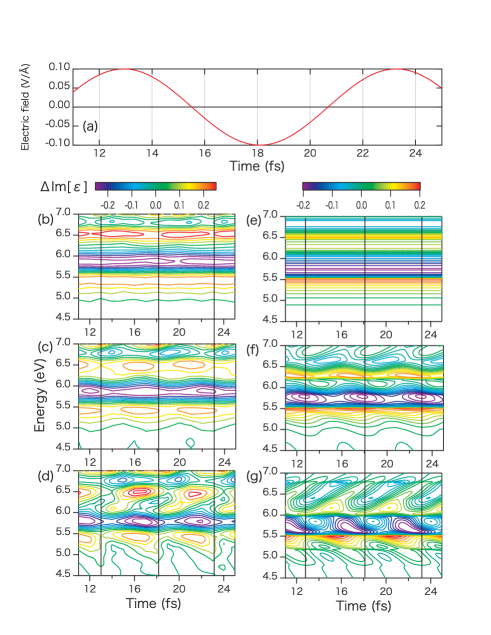
Figure 1: Changes in ${\rm Im}[\varepsilon(T_{p},\omega)]$ ( $\Delta{\rm Im}[\varepsilon(T_{p},\omega)]$) under circularly ((b) and (e)), elliptically ((c) and (f)), and linearly ((d) and (g)) polarized lasers. (b)-(d) show the numerical results from the real-time TDDFT, and (e)-(g) show the results from analytical formulas Eqs. (8), (14), and (15), respectively. Panel (a) shows the electric field of the pump laser. The horizontal axis presents the probe time, whose range corresponds to the simulation by the real-time TDDFT.

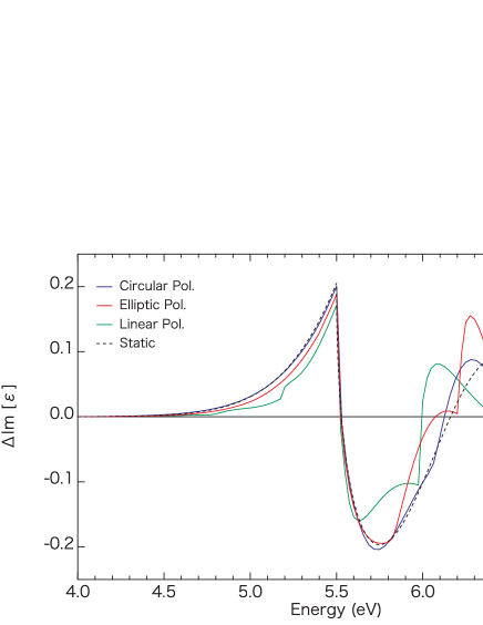
Figure 2: Time-average of the $\Delta{\rm Im}[\varepsilon(T_{p},\omega)]$ under a laser field with frequency of 0.4 eV and a field amplitude 10 MV/cm calculated from Eqs. (8), (14), and (15). For reference, the static FKE calculated by the Tharmalingam formula Tharmalingam63 is represented by the black dashed line.

In this section, we aim to demonstrate the quantitative difference between circular and linear polarization by comparing the numerical results. Diamond is a typical dielectric used in non-linear laser-matter interaction studies, and we selected it as an example with which to illustrate the application of the above formalism.

Figure 1 shows the change in the imaginary part of the dielectric function, $\Delta{\rm Im}[\varepsilon(T_{p},\omega)]$. The maximum field amplitude is 10 MV/cm and the $\Omega$ is 0.4 eV. Figure 1 (b)-(d) show the results from the real-time TDDFT, and (e)-(g) show the results of the analytical theory. We assumed that the band gap, $\varepsilon_{g}$, is 5.5 eV, the reduced mass $\mu$ is 0.25$m_{e}$, and the transition moment $P_{cv}=0.928$ in atomic units for the analytical formulas. We adopt time components of $n=-1,0$, and 1 in Eqs. (8), (14), and (15). The vertical black solid lines in Fig. 1(b)-(g) represent the maximum of the absolute value of the electric field shown in Fig. 1 (a). In numerical simulation by the real-time TDDFT, we assume the pump field rotating in $x$-$z$ plane, which corresponds to $a$- and $c$-axises of diamond, and the polarization of the probe pulse is set to be parallel to $b$-axis.

The Tr-DFKE under circular polarization is presented in Fig. 1 (b) and (e) respectively. As we expected in Eq. (15), the time-dependence of DFKE almost disappears in real-time TDDFT. However, for higher energy region around 6.5 $-$ 7eV, small oscillation of $\Delta{\rm Im}[\varepsilon(T_{p},\omega)]$ can be seen. The ratio of the small oscillation between the peak and dip is approximately 10 %. There are two possible explanations for this modulation. First, the artificial error in real-time simulation is unavoidable. The Tr-DFKE requires high computational accuracy. Therefore, small errors in time evolution and the Fourier transformation affect the result. The second is the anisotropy of the band structure, which changes the definition of the reduced mass $\mu\rightarrow\mu(k,\theta,\phi)$. Although the band structure of diamond is almost isotropic around the $\Gamma$-point, it has a four-fold symmetric structure far from the $\Gamma$-point and higher energy bands. Since the DFKE depends on the reduced mass, time-dependence in circular polarization should include the effect of the structure of the valence and conduction bands.

Figures 1 (c) and (f) show the case of the elliptically polarized laser. The real-time TDDFT shows $2\Omega$ oscillation for all energies. The analytic formula Eq. (8) well reproduces the real-time TDDFT qualitatively for not only the frequency of the oscillation of $\Delta{\rm In}[\varepsilon(T_{p},\omega)]$, but also the phase shift depending on the probe photon energy. The amount of oscillation and the phase shift are weaker than that of the linear polarization shown in Figs. 1 (d) and (g). However, the peaks of the modulation shows the same phase shift under linear polarization.

Figure 2 shows the time-average of $\Delta{\rm Im}[\varepsilon(T_{p},\omega)]$ of each polarization calculated by the analytic formula. The time-average corresponds to the probe by continuous-wave lasers, and depends only on the density of states Jauho96 .

The blue line denoted the case of the circularly polarized laser. The exponential tail below the band gap, which is a feature of the FKE, can be seen. The oscillation above the band gap is due to the response of the different dressed states and the blue shift of the band gap by $U_{c}$. In this case, $U_{c}$ is approximately 0.95 eV, which corresponds to the energy at which $\Delta{\rm Im}[\varepsilon(\omega)]$ has a sharp peak. Since the response of the $l=-1$ dressed state is intense, the apparent blue shift of the band gap becomes 0.5 eV.

The red line denotes the case of the elliptic polarization ($\eta=1/\sqrt{2}$). The most obvious difference is the magnitude of the blue shift. The original band gap is blue-shifted by $U_{e}=0.71$ eV. Although the overall behavior is similar to that of circular polarization, the contribution of the $l_{1}+l_{2}=-1$ dressed band becomes weaker than that of the circular polarization.

The case of linearly polarized light is represented by the green line. Here, $U_{p}$ is 0.5 eV which is consistent with the apparent blue shift of the band gap. There is a small shoulder at 5.1 eV. This energy corresponds to the $l_{1}+l_{2}=-3$ dressed state.

For reference, the numerical result for the static FKE Tharmalingam63 is represented by the black dashed line. Since the applied field amplitude is stable with circular polarization, the tunneling effect is expected to be similar to the static FKE. As expected, the behavior under the band gap agrees with the case of circularly polarized light. However, the oscillation above the band gap is different. This result indicates that the FKE under circularly polarized light is not equivalent to the static FKE, even though the amplitude of the electric field is static. Thus, using the dressed states is indispensable.

V Summary

We presented an analytical formulation for the time-resolved dynamical Franz-Keldysh effect under an elliptically polarized laser. This formula connects the cases of linear polarization and circular polarization though the ellipticity of the pump laser. We found that the time-dependent change in the optical properties observed under linearly polarized light disappears as the ellipticity increases. Therefore, linearly polarized light is suitable for ultrafast control of the material response. On the other hand, the response of the dressed state is still important for understanding the change in the optical properties caused by a circularly polarized light field.

References

- (1) M. Hentschel, R. Klenberger, Ch. Spielmann, G.A. Reider, N. Milosevic, T. Brabec, U. Heinzmann, M. Drescher, and F. Krausz, Nature 414, 509 (2001).
- (2) H. Hirori, A. Doi, F. Blanchard, and K. Tanaka, Appli. Phys. Lett. 98, 091106 (2011).
- (3) A.H. Chin, O.G. Calderon, and J. Kono, Phys.Rev. Lett. 86 , 3292 (2001).
- (4) H.Hirori, K. Shinokita, M. Shirai, S. Tani, Y. Kadoya, and K. Tanaka, Nat. Comm. 2, 594 (2011).
- (5) A. Schiffrin, T. Paasch-Colberg, N. Karpowicz, V. Apalkov, D. Gerster, S. Mühlbrandt, M. Korbman, J. Reichert, M. Schultze, S. Holzner, J.V. Barth, R. Kienberger, R. Ernstorfer, V.S. Yakovlev, M.I. Stockman, and F. Krausz, Nature 493, 70 (2013).
- (6) M. Schultze, E.M. Botschafter, A. Sommer, S. Holzner, W. Schweinberger, M. Fless, M. Hofstetter, R. Kienberger, V. Apalkov, V.S. Yakovlev, M.I. Stockman, F. Krausz, Nature 493, 75 (2013).
- (7) F. Nobelli, D. Fausti, F. Giusti, F. Parmigiani, and M. Hoffmann, Scientific Reports 3 1227 (2013).
- (8) M. Schultze, K. Ramasesha, C.D. Pemmaraju, S.A. Sato, D. Whitmore, A. Gandman, J.S. Prell, L.J. Borja, D. Prendergast, K. Yabana, D.M. Neumark, S.R. Leone, Science 346, 1348 (2014).
- (9) W.Franz, Z. Naturforsch. Teil A 13, 484 (1958).
- (10) L. V. Keldysh, Sov. Phys. JETP 34, 788 (1958).
- (11) K. Tharmalingam, Phys. Rev. 130, 2204 (1963).
- (12) B. O. Seraphin and R. B. Hess, Phys. Rev. Lett. 14, 138 (1965).
- (13) R. E. Nahory and J. L. Shay, Phys. Rev. Lett. 21, 1569 (1968).
- (14) H.Shen, M. Dutta, J. Appl. Phys. 78, 2151 (1995).
- (15) J.K. Wahlstrand, J.E. Sipe, Phys. Rev. B82, 075206 (2010).
- (16) F. Duque-Gomez, J.E. Sipe, J. Phys. Chem. Solids 76, 138 (2015).
- (17) Y. Yacoby, Phys. Rev. 169, 610 (1968).
- (18) A. P. Jauho and K. Johnsen, Phys.Rev. Lett. 76, 4576 (1996).
- (19) K. B. Nordstrom, K. Johnsen, S. J. Allen, A. P. Jauho, B. Birnir, J. Kono, T. Noda, H. Akiyama, and H. Sakaki, Phys. Rev. Lett. 81, 457 (1998).
- (20) A. Srivastava, R. Srivastava, J. Wang, and J. Kono, Phys.Rev.Lett. 93, 157401 (2004).
- (21) Y. Mizumoto, Y. Kayanuma, A. Srivastava, J. Kono, and A. H. Chin, Phys. Rev. B 74, 045216 (2006).
- (22) S. Ghimire, A.D. DiChiara, E. Sistrunk, U.B. Szafruga, P. Agostini, L. F. DiMauro, and D. A. Reis, Phys. Rev. Lett. 107, 167407 (2011).
- (23) T. Otobe, Y. Shinohara, S. A. Sato, and K. Yabana, Phys. Rev. B 93, 045124 (2016).
- (24) M. Lucchini, S. Sato, J. Herrmann, A. Ludwig, M. Volkov, L. Kasmi, Y. Shinohara, K. Yabana, L. Gallmann, and U. Keller, Science 353, 916 (2016).
- (25) K. Uchida, T. Otobe, T. Mochizuki, C. Kim, M. Yoshita, H. Akiyama, L. N. Pfeiffer, K. W. West, K. Tanaka, and H. Hirori, JSAP-OSA Joint Symposia 2015 Abstracts, (Optical Society of America, 2015), paper 15p_2E_10. Paper is submitted.
- (26) W. V. Houston, Phys. Rev. 51, 184 (1940).
- (27) H. R. Reiss and V. P. Krainov, J. Phys. A: Math. Gen. 36, 5575 (2003).
- (28) E. Runge and E. K. U. Gross, Phys.Rev. Lett. 52, 997 (1984).
- (29) G.F. Bertsch, J.-I. Iwata, A. Rubio, and K. Yabana, Phys. Rev. B 62 , 7998 (2000).
- (30) T. Otobe, M. Yamagiwa, J. -I. Iwata, K. Yabana, T. Nakatsukasa, and G. F. Bertsch, Phys. Rev. B77, 165104 (2008).
- (31) N. Troullier and J.L. Martins, Phys. Rev. B 43, 1993 (1991).
- (32) L. Kleinman and D. M. Bylander, Phys. Rev. Lett. 48, 1425 (1982).
- (33) J. P. Perdew and A. Zunger, Phys. Rev. B 23, 5048 (1981).
- (34) K. Yabana and G.F. Bertsch, Phys. Rev. B 54, 4484 (1996).
- (35) K. Yabana, T. Sugiyama, Y. Shinohara, T. Otobe, and G. F. Bertsch, Phys. Rev. B 85, 045134 (2012).