X-ray Fourier ptychographic microscopy

Abstract

Following the recent developement of Fourier ptychographic microscopy (FPM) in the visible range by Zheng et al. (2013), we propose an adaptation for hard x-rays. FPM employs ptychographic reconstruction to merge a series of low-resolution, wide field of view images into a high-resolution image. In the x-ray range this opens the possibility to overcome the limited numerical aperture of existing x-ray lenses. Furthermore, digital wave front correction (DWC) may be used to charaterize and correct lens imperfections. Given the diffraction limit achievable with x-ray lenses (below $100\,\mathrm{nm}$), x-ray Fourier ptychographic microscopy (XFPM) should be able to reach resolutions in the $10\,\mathrm{nm}$ range.

¹Physics Department, Technical University of Denmark, 2800 Kgs. Lyngby, Denmark
²European Synchrotron Radiation Facility, B.P. 220, F-38043 Grenoble Cedex, France

^∗detlefs@esrf.fr

(100.3010) Image reconstruction techniques; (110.4155) Multiframe image processing; (340.7460) X-ray microscopy.

1 Introduction

Recently Zheng et al. [1] demonstrated Fourier ptychographic microscopy (FPM) in the visible wavelength regime. The technique iteratively stiches together a number of variably illuminated, low-resolution intensity images in Fourier space to produce a wide-field, high-resolution complex image of a two-dimensional sample. By varying the angle of the incident light a wide range of scattering angles is covered – thus improving the space-bandwidth product (SBP) [2] – without moving the sample and imaging system.

The image recovery procedure of FPM follows a stragety similar to ptychography (that is, scanning diffraction microscopy, a technique that is now routinely employed in the soft and hard x-ray range) [3, 4, 5, 6, 7, 8, 9]: iteratively solving for a sample estimate that is consistent with many intensity measurements. Unlike ptychography, however, FPM’s object support constraints are imposed in the Fourier domain, offering several unique advantages and opportunities [1].

Zheng et al. employed a conventional optical microscope with small magnification ($\times 2$ objective), limited numerical aperture (NA) 0.08, and large field of view (FOV) $\approx 120\,\mathrm{mm^{2}}$. Their reconstructed FPM image had a maximum synthetic NA of 0.5 [1] set by the maximum angle between the optical axis of the imaging lens and the illuminating beam. The resulting reconstructed image had a resolution comparable to a conventional microscope with $\times 20$ magnification, but the much larger FOV and depth of field (DOF) of the low-magnification microscope.

In the visible range, FPM is particularly useful for increasing the FOV and DOF, as high spatial resolution can already be achieved by using objective lenses with very large numerical aperture. In the x-ray range, however, the resolution is limited by the small numerical aperture of available x-ray lenses and by lens imperfections. Both of these limitations can be addressed by FPM: The compound image corresponds to a larger synthetic aperture, and DWC can be used to correct for lens imperfections in data processing. The reconstruction yields a complex image, i.e. both amplitude and phase contrast are detected. For hard x-rays, phase contrast is usually dominant and (non-magnified) x-ray phase contrast imaging is a growing field [10].

The adaptation of FPM to x-rays is straight-forward. Rather than changing the angle of the incident beam, however, we propose to sample different scattering angles (and thus reciprocal space) by moving the detector and objective lens.

A significant difference between the visual and x-ray regimes is the transmission profile as function of distance from the lens center (pupil function). Lenses for visible light have a pupil function that is completely opaque outside of the aperture, and close to 100% transmission throughout the active area of the lens. For x-ray lenses the pupil function depends on the type of lens employed: For a (hard x-ray) zone plate (ZP) [11] with dominant phase contrast the pupil function is similar to a visible lens, whereas for a (soft x-ray) ZP with dominant absorption contrast opaque and transparent zones alternate. Compound refractive lenses (CRLs) [12], finally, have a Gaussian pupil function eventually terminated by an opaque limiting aperture (physical aperture, to be distinguished from the equivalent aperture). These characteristic pupil functions can easily be taken into account in the reconstruction algorithm, as we show below.

2 Wave propagation and image formation with plane wave illumination

The aim of the experiment is to determine the complex filter function $s(x_{0},y_{0})$ representing the sample, eq. 10. For convenience, numerical efficiency and stability, the reconstruction is performed on the Fourier transform, $S^{\prime}(u_{0},v_{0})$, see eq. 28, of a phase shifted sample function $s^{\prime}(x_{0},y_{0})=\exp\left[\frac{i\pi}{\lambda d_{1}}(x_{0}^{2}+y_{0}^{2})\right]\cdot s(x_{0},y_{0})$, see eq. 24.

The (phase shifted) wave field in the detector plane, $g^{\prime}(x_{2},y_{2})$, see eq. 34), is obtained by shifting according to the angle of the incident wave front (eq. 27), multiplication with the pupil function (eq. 16), and inverse Fourier transformation,

$$g^{\prime(\theta,\chi)}(x_{2},y_{2})={\cal F}^{-1}_{u_{2},v_{2}\rightarrow x_{2},y_{2}}\left[p(-\lambda d_{2}u_{2},-\lambda d_{2}v_{2})\cdot S^{\prime}\left(-\frac{d_{2}}{d_{1}}u_{2}-\frac{\theta}{\lambda},-\frac{d_{2}}{d_{1}}v_{2}-\frac{\chi}{\lambda}\right)\right]$$ (1)

In order to update the Fourier map of the sample, $S^{\prime}$, with data from the measured intensities we take the Fourier transform of eq. 34,

$$G^{\prime(\theta,\chi)}(u_{2},v_{2}) = p(-\lambda d_{2}u_{2},-\lambda d_{2}v_{2})\cdot S^{\prime}\left(-\frac{d_{2}}{d_{1}}u_{2}-\frac{\theta}{\lambda},-\frac{d_{2}}{d_{1}}v_{2}-\frac{\chi}{\lambda}\right)$$ (2)

Eq. 2 can be used to update the Fourier map of the sample $S^{\prime}(u_{0},v_{0})$.

$$S^{\prime}_{\mathrm{new}}(u_{0},v_{0}) = p^{*}(\lambda d_{1}u_{0}+\theta d_{1},\lambda d_{1}v_{0}+\chi d_{1})\cdot G^{\prime}\left(-\frac{d_{1}}{d_{2}}\left(u_{0}+\frac{\theta}{\lambda}\right),-\frac{d_{1}}{d_{2}}\left(v_{0}+\frac{\chi}{\lambda}\right)\right)$$ (3)

$$+\left(1-\left|p\left(\lambda d_{1}u_{0}+\theta d_{1},\lambda d_{1}v_{0}+\chi d_{1}\right)\right|^{2}\right)\cdot S^{\prime}_{\mathrm{old}}(u_{0},v_{0}).\ \ \ \ \$$

By multiplying with $p^{*}$ we remove any possible phase shift introduced by the pupil function and enforce the “support”, i.e. remove any artifacts in $G^{\prime}$ outside of the physical aperture of the lens (see eq. 18). The second term in eq. 3 ensures that information outside the pupil function is not affected by the update (for areas where $p=0$) and that the Fourier amplitude does not decay during subsequent cycles (for areas where $0<\left|p\right|<1$, which naturally occur with absorbing refractive lenses). Note that substituting eq. 2 in eq. 3 without injection of measured information into $G^{\prime}$ results in $S^{\prime}_{\text{new}}=S^{\prime}_{\text{old}}$.

In the final step of the algorithm, the complex real space map of the sample, $s$, is obtained by inverse Fourier transform of $S^{\prime}$ (eq. 28) and removal of the phase shift, see eq. 24.

$$s(x_{0},y_{0}) = \exp\left[-\frac{i\pi}{\lambda d_{1}}(x_{0}^{2}+y_{0}^{2})\right]{\cal F}^{-1}_{u_{0},v_{0}\rightarrow x_{0},y_{0}}\left[S^{\prime}(u_{0},v_{0})\right]$$ (4)

$$= \exp\left[-\frac{i\pi}{\lambda d_{1}}(x_{0}^{2}+y_{0}^{2})\right]\iint\exp\left[i2\pi(u_{0}x_{0}+v_{0}y_{0})\right]S^{\prime}(u_{0},v_{0})\operatorname{d}\!{u_{0}}\operatorname{d}\!{v_{0}}$$ (5)

3 Ptychographic algorithm

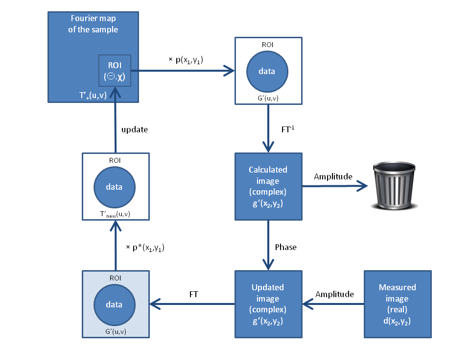
Figure 1: Schematic outline of the Fourier ptychography algorithm.

The ptychography algorithm (see Fig. 1) starts by initializing the Fourier representation of the sample, $S^{\prime}(u_{0},v_{0})$ with more or less arbitrary values. The following steps are then repeated until convergence is achieved:

• For each pair of detection angles ($\theta,\chi$) the product $G^{\prime}$ of the sample’s Fourier map $S$ and the pupil function $p$ is calculated, eq. 2. As the physical aperture of the pupil function is significantly smaller than the complete Fourier map of the sample these calculations are best carried out on a region of interest matched to the physical aperture.

• The complex detector field $g^{\prime}(x_{2},y_{2})$ is obtained from $G^{\prime}$ by inverse Fourier transform (eq. 34).

• The resulting wave field $g^{\prime}(x_{2},y_{2})$ is then split into amplitude and phase. The amplitude is replaced by the square root of the corresponding measured intensity, $d(x_{2},y_{2})$.

• The resulting “new” wave field $g^{\prime}(x_{2},y_{2})$ is Fourier-transformed to $G^{\prime}$.

• The “support” is applied and possible phase shifts of the pupil function are removed by multiplication with $p^{*}$, see eq. 3.

• The Fourier map of the sample $S^{\prime}_{(}u_{0},v_{0})$ is modified using eq. 3.

Note that in this algorithm it makes absolutely no difference whether the original ($g(x_{2},y_{2})$) or phase-shifted ($g^{\prime}(x_{2},y_{2})$) image wave field is used.

4 Digital Wavefront Correction

Unlike classical ptychography, our treatment does not allow us to distinguish effects coming from the sample and from the incident beam. However, it should be possible to refine the pupil function $p(x_{1},y_{1})$ once the ptychographic reconstruction has converged, e.g. by systematically comparing the wave field $Q$ calculated from the measured data and the final Fourier map of the sample.

5 Convergent beam illumination

In the case of plane wave illumination discussed above, the reconstruction is performed on the Fourier transform, $S^{\prime}(u_{0},v_{0})$, see eq. 28, of a phase shifted sample function $s^{\prime}(x_{0},y_{0})$.

The phase, $\Phi=\frac{pi}{\lambda d_{1}}(x_{0}^{2}+y_{0}^{2})$, see eq. 24, is benign and often negligible in the visible range. In the hard x-ray range, however, it can become vicious.

A typical setup for hard x-ray microscopy using refractive lenses could be $\lambda=0.1\,\mathrm{nm}$, $d_{1}=10\,\mathrm{cm}$, $x_{0,\textrm{max}},y_{0,\mathrm{max}}=100\,\mathrm{\mu m}$, with effective pixel size $\delta x_{0}=\delta y_{0}=100\,\mathrm{nm}$. This results in a maximum phase, in the corner of the image of $\Phi_{\textrm{max}}=10^{3}\cdot 2\pi$, and a maximum phase jump between adjacent pixels of $\delta\Phi=2\pi$ – in the corner of the image, the phase of a single pixel is no longer well defined. The increased resolution (smaller effective pixel size) of the reconstructed image somewhat alleviates this problem, but the phase drift within pixels remains problematic.

For similar experiments with Fresnel zone plates or multi-layer Laue lenses, the working distance $d_{1}$ would be even smaller, $d_{1}~{}2\,\mathrm{cm}$, such that the maximum phase and phase jump are proportionally higher.

It therefore appears prudent to eliminate this phase factor by introducing the opposite phase shift in the illuminating beam, i.e. by using a convergent beam that is focused onto the plane of the objective lens. In this case the sample function is given directly by $s^{\prime}(x_{0},y_{0})$.

6 Conclusions

We have shown that XFPM offers many exciting possibilities for extending the resolution limit of full-field x-ray microscopy.

Digital wave front correction can be used to take into account the characteristic transmission profiles and manufacturing imperfections of x-ray lenses.

Furthermore, the phase and amplitude profiles obtained from the DWC can be used to characterize the x-ray lens and its defects and thus aid in optimizing the manufacturing process.

Appendix A Definitions

All calculations are carried out in the paraxial approximation, i.e. all vectors are nearly parallel to the $z$ direction. The sample, lens, and detector are positioned parallel to the $x$–$y$ plane at $z=0$ (sample), $z=d_{1}$ (lens) and $z=d_{1}+d_{2}$ (image/detector).

A.1 Fourier Transform

We denote functions in direct space by lower case letters, and functions in Fourier space by upper case letters.

$$G(u,v)={\cal F}_{x,y\rightarrow u,v}[g(x,y)]=\iint\exp\left[-i2\pi(ux+vy)\right]\cdot g(x,y)\operatorname{d}\!{x}\operatorname{d}\!{y},$$ (6)

and

$$g(x,y)={\cal F}^{-1}_{u,v\rightarrow x,y}[G(u,v)]=\iint\exp\left[i2\pi(ux+vy)\right]\cdot G(u,v)\operatorname{d}\!{u}\operatorname{d}\!{v}.$$ (7)

All integrals are taken from $-\infty$ to $\infty$.

A.2 Incident wave field

Let the incident wave field have uniform amplitude and phase, $t(\vec{r})=\exp\left[i\vec{k}\cdot\vec{r}\right]$. Let the wave vector of the incident wave field be

$$\vec{k}=\left(\begin{array}[]{c}{k_{x}}\\ {k_{y}}\\ {k_{z}}\end{array}\right)\approx k\left(\begin{array}[]{c}{\theta}\\ {\chi}\\ {1}\end{array}\right),$$ (8)

where $k=2\pi/\lambda$, $\lambda$ is the wave length, and $\theta,\chi\ll 1$ are the beam angles in the horizontal and vertical, respectively.

The sample at position $z=0$ is thus illuminated by the wave field

$$t_{-}^{(\theta,\chi)}(x_{0},y_{0})=\exp\left[ik(\theta x_{0}+\chi y_{0})\right]$$ (9)

A.3 Sample

Let the sample be represented by the complex filter function $s(x_{0},y_{0})$. The wave field just downstream of the sample is thus

$$t_{+}^{(\theta,\chi)}(x_{0},y_{0})=t_{-}^{(\theta,\chi)}(x_{0},y_{0})\cdot s(x_{0},y_{0}).$$ (10)

Thus with perpendicular illumination, $\theta=\chi=0$, the wave field just downstream of the sample is simply the sample filter function, $t_{+}^{(0,0)}(x_{0},y_{0})=s(x_{0},y_{0})$.

The Fourier transform of this field is given by

$$T_{+}^{(\theta,\chi)}(u_{0},v_{0})={\cal F}_{x_{0},y_{0}\rightarrow u_{0},v_{0}}\left[t_{+}^{(\theta,\chi)}(x_{0},y_{0})\right]$$ (11)

$$= \iint\exp\left[-i2\pi(u_{0}x_{0}+v_{0}y_{0})\right]\cdot t_{+}^{(\theta,\chi)}(x_{0},y_{0})\operatorname{d}\!{x_{0}}\operatorname{d}\!{y_{0}}$$ (12)

$$= \iint\exp\left[-i2\pi(u_{0}x_{0}+v_{0}y_{0})\right]\cdot\exp\left[i2\pi\left(\frac{\theta}{\lambda}x_{0}+\frac{\chi}{\lambda}y_{0}\right)\right]\cdot s(x_{0},y_{0})\operatorname{d}\!{x_{0}}\operatorname{d}\!{y_{0}}$$ (13)

$$= {\cal F}_{x_{0},y_{0}\rightarrow u_{0}-\frac{\theta}{\lambda},v_{0}-\frac{\chi}{\lambda}}\left[s(x_{0},y_{0})\right]$$ (14)

$$= S\left(u_{0}-\frac{\theta}{\lambda},v_{0}-\frac{\chi}{\lambda}\right),$$ (15)

with $S(u_{0},v_{0})={\cal F}_{x_{0},y_{0}\rightarrow u_{0},v_{0}}[s(x_{0},y_{0})]$.

Changing the angle of incidence corresponds to a shift in Fourier space, as noted by Zheng et al [1].

A.4 Lens

Let the lens be positioned at $z=d_{1}$. Let the lens be described by the function

$$l(x_{1},y_{1})=p(x_{1},y_{1})\cdot\exp\left[-ik\frac{x_{1}^{2}+y_{1}^{2}}{2f}\right],$$ (16)

where $f$ is the focal length with $1/f=1/d_{1}+1/d_{2}$.

The pupil function $p(x_{1},y_{1})$ may be complex, e.g. to compensate for a some defocussing or small lens errors. However, we require that its magnitude is less or equal to unity,

$$\left|p(x_{1},y_{1})\right|\leq 1,$$ (17)

and that it vanishes for $x_{1},y_{1}$ outside of the physical aperture of the lens, e.g. for a circular lens with physical radius $R$:

$$p(x_{1},y_{1})=0;\text{ for }x_{1}^{2}+y_{1}^{2}>R^{2}.$$ (18)

This requirement provides the “support” for the ptychography algorithm by defining a limited region of interest in the Fourier map of the sample that affects the image for any given angle of illumination (and vice versa), see below.

A.5 Image

Let the wave field at the image plane ($z=d_{1}+d_{2}$) be $g(x_{2},y_{2})$. Evaluating the paraxial diffraction integral for the propagation from the sample to the lens, and then to the detector plane yields

$$g(x_{2},y_{2})=$$ (22)

$$= \frac{1}{i\lambda d_{2}}\iint\exp\left[\frac{i\pi}{\lambda d_{2}}\left((x_{2}-x_{1})^{2}+(y_{2}-y_{1})^{2}\right)\right]\cdot l(x_{1},y_{1})$$

$$\cdot\left(\frac{1}{i\lambda d_{1}}\iint\exp\left[\frac{i\pi}{\lambda d_{1}}\left((x_{1}-x_{0})^{2}+(y_{1}-y_{0})^{2}\right)\right]\cdot t_{+}(x_{0},y_{0})\operatorname{d}\!{x_{0}}\operatorname{d}\!{y_{0}}\right)\operatorname{d}\!{x_{1}}\operatorname{d}\!{y_{1}}$$

$$= \frac{-1}{\lambda^{2}d_{1}d_{2}}\exp\left[\frac{i\pi}{\lambda d_{2}}\left(x_{2}^{2}+y_{2}^{2}\right)\right]\iint\exp\left[\frac{-i2\pi}{\lambda d_{2}}\left(x_{2}x_{1}+y_{2}y_{1}\right)\right]\cdot p(x_{1},y_{1})$$

$$\cdot\left(\iint\exp\left[\frac{-i2\pi}{\lambda d_{1}}\left(x_{1}x_{0}+y_{1}y_{0}\right)\right]\exp\left[\frac{i\pi}{\lambda d_{1}}\left(x_{0}^{2}+y_{0}^{2}\right)\right]\cdot t_{+}(x_{0},y_{0})\operatorname{d}\!{x_{0}}\operatorname{d}\!{y_{0}}\right)\operatorname{d}\!{x_{1}}\operatorname{d}\!{y_{1}}\ \ \ \ \$$

$$= -\frac{d_{1}}{d_{2}}\exp\left[\frac{i\pi}{\lambda d_{2}}\left(x_{2}^{2}+y_{2}^{2}\right)\right]\iint\exp\left[-i2\pi\left(x_{2}\frac{d_{1}}{d_{2}}u_{0}+y2\frac{d_{1}}{d_{2}}v_{0}\right)\right]\cdot p(\lambda d_{1}u_{0},\lambda d_{1}v_{0})$$

$$\cdot\left(\iint\exp\left[-i2\pi\left(x_{0}u_{0}+y_{0}v_{0}\right)\right]\exp\left[\frac{i\pi}{\lambda d_{1}}\left(x_{0}^{2}+y_{0}^{2}\right)\right]\cdot t_{+}(x_{0},y_{0})\operatorname{d}\!{x_{0}}\operatorname{d}\!{y_{0}}\right)\operatorname{d}\!{u_{0}}\operatorname{d}\!{v_{0}}\ \ \ \ \$$

$$= -\frac{d_{1}}{d_{2}}\exp\left[\frac{i\pi}{\lambda d_{2}}\left(x_{2}^{2}+y_{2}^{2}\right)\right]\iint\exp\left[-i2\pi\left(x_{2}\frac{d_{1}}{d_{2}}u_{0}+y2\frac{d_{1}}{d_{2}}v_{0}\right)\right]\cdot p(\lambda d_{1}u_{0},\lambda d_{1}v_{0})$$

$$\cdot{\cal F}_{x_{0},y_{0}\rightarrow u_{0},v_{0}}\left[\exp\left[\frac{i\pi}{\lambda d_{1}}\left(x_{0}^{2}+y_{0}^{2}\right)\right]\cdot t_{+}(x_{0},y_{0})\right]\operatorname{d}\!{u_{0}}\operatorname{d}\!{v_{0}}\ \ \ \ \$$

For ease of notation we define a phase-shifted wave field at the sample position and the corresponding phase-shifted sample field

$$t^{\prime}_{+}(x_{0},y_{0}) = \exp\left[\frac{i\pi}{\lambda d_{1}}\left(x_{0}^{2}+y_{0}^{2}\right)\right]\cdot t_{+}(x_{0},y_{0})$$ (23)

$$s^{\prime}(x_{0},y_{0}) = \exp\left[\frac{i\pi}{\lambda d_{1}}(x_{0}^{2}+y_{0})^{2}\right]\cdot s(x_{0},y_{0})$$ (24)

A change of the incident beam direction leads to a shift in the Fourier transform of the wave field at the sample position, $T^{\prime}_{+}$ (eq. 15),

$$T^{\prime(\theta,\chi)}_{+}(u_{0},v_{0})$$ (25)

$$= {\cal F}_{x_{0},v_{0}\rightarrow u_{0},v_{0}}\left[t^{\prime}_{+}(x_{0},y_{0})\right]$$

$$= \iint\exp\left[-i2\pi(u_{0}x_{0}+v_{0}y_{0})\right]\exp\left[\frac{i\pi}{\lambda d_{1}}(x_{0}^{2}+y_{0}^{2})\right]s(x_{0},y_{0})\exp\left[ik(\theta x_{0}+\chi y_{0})\right]\operatorname{d}\!{x_{0}}\operatorname{d}\!{y_{0}}\ \ \ \ \ \ \ \$$ (26)

$$= S^{\prime}\left(u_{0}-\frac{\theta}{\lambda},v_{0}-\frac{\chi}{\lambda}\right),$$ (27)

where

$$S^{\prime}(u_{0},v_{0}) = {\cal F}_{x_{0},y_{0}\rightarrow u_{0},v_{0}}\left[s^{\prime}(x_{0},y_{0})\right]$$ (28)

$$= \iint\exp\left[-i2\pi(u_{0}x_{0}+v_{0}y_{0})\right]\left(\exp\left[\frac{i\pi}{\lambda d_{1}}(x_{0}^{2}+y_{0})^{2}\right]s(x_{0},y_{0})\right)\operatorname{d}\!{x_{0}}\operatorname{d}\!{y_{0}}$$ (29)

Inserting these relations into eq. 22 we find

$$g(x_{2},y_{2}) = -\frac{d_{1}}{d_{2}}\exp\left[\frac{i\pi}{\lambda d_{2}}\left(x_{2}^{2}+y_{2}^{2}\right)\right]\iint\exp\left[-i2\pi\left(x_{2}\frac{d_{1}}{d_{2}}u_{0}+y_{2}\frac{d_{1}}{d_{2}}v_{0}\right)\right]$$ (32)

$$\cdot p(\lambda d_{1}u_{0},\lambda d_{1}v_{0})\cdot T^{\prime}_{+}(u_{0},v_{0})\operatorname{d}\!{u_{0}}\operatorname{d}\!{v_{0}}\ \ \ \ \$$

$$= -\frac{d_{2}}{d_{1}}\exp\left[\frac{i\pi}{\lambda d_{2}}\left(x_{2}^{2}+y_{2}^{2}\right)\right]\iint\exp\left[i2\pi\left(x_{2}u_{2}+y_{2}v_{2}\right)\right]$$

$$\cdot p(-\lambda d_{2}u_{2},-\lambda d_{2}v_{2})\cdot T^{\prime}_{+}\left(-\frac{d_{2}}{d_{1}}u_{2},-\frac{d_{2}}{d_{1}}v_{2}\right)\operatorname{d}\!{u_{2}}\operatorname{d}\!{v_{2}}\ \ \ \ \$$

$$= -\frac{d_{2}}{d_{1}}\exp\left[\frac{i\pi}{\lambda d_{2}}\left(x_{2}^{2}+y_{2}^{2}\right)\right]$$

$$\cdot{\cal F}^{-1}_{u_{2},v_{2}\rightarrow x_{2},y_{2}}\left[p(-\lambda d_{2}u_{2},-\lambda d_{2}v_{2})\cdot T^{\prime}_{+}\left(-\frac{d_{2}}{d_{1}}u_{2},-\frac{d_{2}}{d_{1}}v_{2}\right)\right],$$

We have thus obtained a relation between the observed wave field, $g$, and the Fourier transform of the sample, $S$, via the phase-shifted field $T^{\prime}_{+}$.

The detector is sensitive only to the intensity, $\left|g(x_{2},y_{2})\right|^{2}$, therefore the phase factor $\exp\left[\frac{i\pi}{\lambda d_{2}}(x_{2}^{2}+y_{2}^{2})\right]$ in eq. 32 does not influence the measurements. We absorb it, together with the constant amplitude factor $-d_{2}/d_{1}$ due to the magnification of the image into the effective field $g^{\prime}(x_{2},y_{2})$.

$$g^{\prime}(x_{2},y_{2}) = -\frac{d_{1}}{d_{2}}\exp\left[\frac{-i\pi}{\lambda d_{2}}\left(x_{2}^{2}+y_{2}^{2}\right)\right]\cdot g(x_{2},y_{2})$$ (33)

$$= {\cal F}^{-1}_{u_{2},v_{2}\rightarrow x_{2},y_{2}}\left[p(-\lambda d_{2}u_{2},-\lambda d_{2}v_{2})\cdot S^{\prime}\left(-\frac{d_{2}}{d_{1}}u_{2}-\frac{\theta}{\lambda},-\frac{d_{2}}{d_{1}}v_{2}-\frac{\chi}{\lambda}\right)\right]$$ (34)

Eq. 34 is our final result for calculating the image from the product of the direct space pupil function, $p$ (with suitably scaled arguments), and the Fourier transform of the phase-shifted sample field, $S^{\prime}$.

Appendix B Array sizes, units and pixels

The units of all real space variables ($x,y$) are in meters while all Fourier space variables ($u,v$) are in inverse meters. Angles are in radians and wave fields in both real and Fourier space are unitless. The pupil function is also unitless.

Array sizes are estimated as follows (for simplicity we assume $x$ and $y$ to be identical):

• Let the detector (represented by the array $d$) have $N_{d}$ pixels of size $\Delta x_{2}=a$, giving a field of view $x_{2,\mathrm{max}}=N_{d}a$.

  Typical values are $N_{d}=1000$ and $a=1\,\mathrm{\mu m}$.

• The complex detector field $g^{\prime}$ has to be compared directly to the detected amplitude $d$. Arrays size and pixel size of $g^{\prime}$ and $d$ should therefore be identical, $N_{g}=N_{d}$.

• The FT of $g^{\prime}$ has pixel size $\Delta{u_{2}}=1/x_{2,\mathrm{max}}=1/(N_{g}a)$. As $Q(\mu u_{2},\mu v_{2})$ is the scaled FT of $g^{\prime}$, the array $Q$ has pixel size $\Delta u_{0}=\Delta(\mu u_{2})=\mu/(N_{g}a)$ and field of view $u_{0,\mathrm{max}}=\mu u_{2,\mathrm{max}}=\mu/a$. $N_{Q}=N_{g}$.

  Typical values (for a typical magnification $\mu=10$) are pixel size $\Delta u_{0}=\Delta(\mu u_{2})=10^{4}\,\mathrm{m^{-1}}$ and thus field of view $u_{0,\mathrm{max}}(\mu u)_{2,\mathrm{max}}=10^{7}\,\mathrm{m^{-1}}$.

• The array $p$ has pixel size $\Delta x_{1}=\Delta(\mu u)d_{1}\lambda=\mu d_{1}\lambda/(N_{g}a)$. $N_{p}=N_{Q}=N_{g}$

  A typical value is ($d_{1}=0.33\,\mathrm{m}$) $3.3\cdot 10^{-7}\,\mathrm{m}$, with field of view $330\,\mathrm{\mu m}$ (compared to typical Be lenses with effective apertures of $R\approx 300\,\mathrm{\mu m}$).

• Angular shifts should be $\theta$ several times the physical aperture $R$ divided by the sample-lens distance $d_{1}$, $\theta\approx M\cdot R/d_{1}\approx M\cdot 3.3^{-4}\,\mathrm{m}/(0.33\,\mathrm{m})=M\cdot 1\,\mathrm{mrad})$.

  The corresponding shift in Fourier space is $M\cdot\theta/\lambda\approx M\cdot 10^{-3}/(10^{-10}\,\mathrm{m})=M\cdot 10^{7}\,\mathrm{m^{-1}}$ (consistent with the value for the field of view found above).

• Adding the shift in Fourier space to the field of view of $Q$ yields the full size of the Fourier map of the sample, $S$, i.e. $(M+1)\times$ the Field of view of $Q$ for a shift by $M$ times the physical aperture $R$.

  As the pixel size in $S$ is the same as in $Q$, the number of pixels in $S$ has to be $N_{s}=(M+1)N_{g}$.

• The corresponding resolution of the sample in real space is $1/(N_{s}\Delta(\mu u))=a/((M+1)\mu)$.