caption \addtokomafontcaptionlabel \setcapmargin2em \setcapmargin.75em \setcapindent0pt \manualmark\markleftMedian-of- Jumplists and Dangling-Min BSTs\automark*[section]
Median-of- Jumplists and Dangling-Min BSTs††thanks: The last author is supported by the Natural Sciences and Engineering Research Council of Canada and the Canada Research Chairs Programme.
Abstract
We extend randomized jumplists introduced by Brönnimann, Cazals, and Durand [2] to choose jump-pointer targets as median of a small sample for better search costs, and present randomized algorithms with expected time complexity that maintain the probability distribution of jump pointers upon insertions and deletions. We analyze the expected costs to search, insert and delete a random element, and we show that omitting jump pointers in small sublists hardly affects search costs, but significantly reduces the memory consumption.
We use a bijection between jumplists and “dangling-min BSTs”, a variant of (fringe-balanced) binary search trees for the analysis. Despite their similarities, some standard analysis techniques for search trees fail for dangling-min trees (and hence for jumplists).
1 Introduction
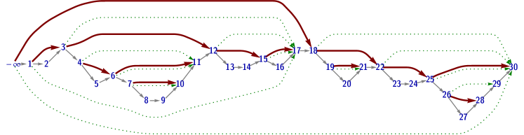
Jumplists were introduced by Brönnimann, Cazals, and Durand [2] as a simple randomized comparison-based dictionary implementation. They allow iteration over the stored elements in sorted order and supports queries and updates in expected logarithmic time. The core is a sorted (singly-) linked listed augmented with jump pointers, i. e., shortcuts that speed up searches. Jump-pointers are required to be well-nested, i. e., they may not cross. This allows binary-search-like navigation. Fig. 1 shows an exemplary jumplist; a detailed definition is deferred to § 3.
If all jump pointers point to the middle of their sublist, we obtain perfect binary search, but we need a rule that is also efficiently maintainable upon insertions and deletions. Brönnimann, Cazals, and Durand [2] proposed a randomized solution: jump pointers invariably have a uniform distribution over their sublist, i. e., the first jump pointer equally likely points to any element and thereby divides the list in two parts, the next- and jump-sublists. Both follow the same rule recursively; since pointers may not cross, they can do so independently.
In this article, we generalize jumplists to use a more balanced distribution: each jump pointer points to the median of a small sample of elements of its sublist. (The original jumplists correspond to .) Building on the algorithms from [2] we present expected-time insertion and deletion algorithms for median-of- jumplists that maintain this more balanced distribution. Here counts the number of keys currently stored. A larger balances the structure more rigidly which improves searches, but makes the cleanup after updates more expensive. Our main contribution is an analysis of median-of- jumplists that precisely quantifies the influence of on searches, insertions and deletions.
We also introduce a novel search strategy (named spine search) that reduces the number of needed key comparisons significantly, and we suggest a further modification of jumplists: for sublists smaller than a threshold , we omit the jump pointers altogether. This allows to trade space for time: elements in these small sublists do not have to store a jump pointer, but the corresponding subfile can only be searched sequentially. We show that this saves a constant fraction of the pointers while affecting expected search costs only by an additive constant.
Outline of the paper
In the remainder of the introduction we summarize related work. § 2 contains common notation and preliminaries used later. In § 3, we define jumplists. We present our spine search strategy in § 4. § 5 introduces the median-of- extension, and § 6 describes the insertion and deletion algorithms. Our analysis is given in § 7, and we conclude the paper with a discussion of the results (§ 8). The appendix contains a list of used notations, as well as details on the operations and omitted parts of the analysis.
1.1 Related Work
(Unbalanced) binary search trees (BSTs) perform close to optimal on average and with high probability when keys are inserted in random order [14, 15]. A standard approach is to enforce the average behavior through randomization. The most direct application of this paradigm is given by Martínez and Roura [16] who devised efficient randomized insert and delete operations that maintain the shape distribution of random insertions. The idea also works when duplicate keys are allowed [20].
Randomized BSTs store subtree sizes for maintaining the distribution. The treaps of Seidel and Aragon [24] instead store a random priority with each node. Treaps remain in random shape by enforcing a heap order w. r. t. the random priorities. Their performance characteristics are very similar to randomized BSTs.
Unless further memory is used, BSTs do not offer time successor queries. Like jumplists, Pugh’s skip lists [22] are augmented, sorted linked lists, so successors are found by following one pointer. Skip lists extend the list elements by towers of pointers of different heights, where each tower cell points to the successor among all element of at least this height. With geometrically distributed heights, operations run in expected time with extra pointers in expectation. The varying tower heights can be inconvenient; this originally motivated the introduction of jumplists. For skip lists, there is a direct and transparent bijection to BSTs [4]; this becomes more complicated for jumplists (see § 3).
The classic alternative to randomization are deterministically balanced BSTs [1]. Munro, Papadakis, and Sedgewick [17] transfer the height-balance rule of 2-3 trees to skip lists, and Elmasry [6] applied the weight-balancing criterion of trees [19] to jumplists. Note that the latter achieves logarithmic update time only in an amortized sense.
A constant-factor speedup over BSTs is achieved with fringe-balanced BSTs. The name originates from fringe analysis, a technique used in their analysis [21].111 The concept appears under a handful of other names in the (earlier) literature: locally balanced search trees [25], diminished trees [9], and iR / SR trees [12, 13]. In a fringe-balanced search tree, leaves collect keys in a buffer. Once a leaf holds keys, it is split: the median of the elements is used as the key of a new node; two new leaves holding the other elements form its subtrees. Many parameters like expected path length, height and profiles of fringe-balanced trees have been studied [5].
2 Notation and Preliminaries
We introduce some important notation here; Appendix A gives a comprehensive list. We use Iverson’s bracket to mean if is true and otherwise. Falling resp. rising factorial powers are denoted by and ; for negative holds resp. . denotes the probability of event and the expectation of random variable . We write to denote equality in distribution.
For a self-contained presentation, we list here a few mathematical preliminaries used in the analysis later.
Beta distribution
The beta distribution has two parameters and is written as . If , we have and has the density
where is the beta function.
The following lemma is helpful for computing expectations involving such beta distributed variables; it is a special case of [26, Lemma 2.30].
Lemma 2.1 (“Powers-to-Parameters”):
Let be a distributed random variable and write . Let further with be given and abbreviate and . Then for an arbitrary (real-valued, measurable) function holds
where is distributed.
Beta-Binomial Distribution
The beta-binomial distribution is a discrete distribution with parameters and . It is written as . If , we have and
(Recall that is zero unless .) An alternative representation of the weights for with is
which yields a combinatorial interpretation.
There is a second way to obtain beta-binomial distributed random variables: we first draw a random probability according to a beta distribution, and then use this as the success probability of a binomial distribution, i. e., conditional on . The beta-binomial distribution is thus also called a mixed binomial distribution, using a beta-distributed mixer ; this explains its name.
Since the binomial distribution is sharply concentrated, one can use Chernoff bounds on beta binomial variables after conditioning on the beta distributed success probability. That already implies that converges to (in a specific sense). We can obtain the stronger error bounds given in the following lemma by directly comparing the probability density functions.
Lemma 2.2 (Local limit law [26, Lem. 2.38]):
Let be a sequence of random variables where is distributed like for . Then for we have uniformly for that
| (1) |
where is the density function of the beta distribution with parameters and .
Since is a polynomial in , it is in particular bounded and Lipschitz continuous in the closed domain . Hence, the local limit law also holds for the random variables for constants and . Further properties of the beta-binomial distribution are collected in [26, § 2.4.7].
The following expectations are listed here for reference; proofs are given in Appendix D.
Lemma 2.3:
Let for and . Then we have with that
Lemma 2.4:
For we have (with )
Hölder continuity
A function defined on a bounded interval is Hölder continuous with exponent when
Hölder continuity is a notion of smoothness that is stricter than (uniform) continuity, but slightly more liberal than Lipschitz continuity (which corresponds to ). with is a stereotypical function that is Hölder continuous (for any ), but not Lipschitz.
For functions defined on a bounded domain, Lipschitz continuity implies Hölder continuity and Hölder continuity with exponent implies Hölder continuity with exponent . Recall that a real-valued function is Lipschitz if its derivative is bounded.
2.1 The Distributional Master Theorem
To solve the recurrences in § 7, we use the “distributional master theorem” (DMT) [26, Thm. 2.76], reproduced below for convenience. It is based on Roura’s continuous master theorem [23], but reformulated in terms of distributional recurrences in an attempt to give the technical conditions and occurring constants in Roura’s original formulation a more intuitive, stochastic interpretation. We start with a bit of motivation for the latter.
The DMT is targeted at divide-and-conquer recurrences where the recursive parts have a random size. The average-case analyses of Quicksort and binary search trees are typical examples that lead to such recurrences. Because of the random subproblem sizes, a traditional recurrence for expected costs has to sum over all possible subproblem sizes, weighted appropriately. That way, the direct correspondence between the recurrence and the algorithmic process is lost, in particular the number of recursive applications is no longer directly visible.
An alternative that avoids this is a distributional recurrence that describes the full distribution of costs. The distribution for larger problem sizes is described by a “toll term” (for the divide and/or combine step) plus the contributions of recursive applications. Such a distributional formulation requires the toll costs and subproblem sizes to be stochastically independent of the recursive costs when conditioned on the subproblem sizes. In typical applications, this is fulfilled when the studied algorithm guarantees that the subproblems on which it calls itself recursively are of the same nature as the original problem. Such a form of randomness preservation is also required for the analysis using traditional recurrences. We can thus use the distributional language to describe costs directly mimicking the structure of our algorithms in this paper.
The DMT allows us to compute an asymptotic approximation of the expected costs directly from the distributional recurrence. Intuitively speaking, it is applicable whenever the relative subproblem sizes of recursive applications converge to a (non-degenerate) limit distribution as (in a suitable sense; see Equation (3) below). The local limit law provided by Lem. 2.2 gives exactly such a limit distribution.
Theorem 2.5 (DMT [26, Thm. 2.76]):
Let be a family of random variables that satisfies the distributional recurrence
| (2) |
where the families are independent copies of , which are also independent of , and . Define , , and assume that they fulfill uniformly for
| (3) |
as for a constant and a Hölder-continuous function . Then is the density of a random variable and .
Let further
| (4) |
as for a function and require that is also Hölder continuous on . Moreover, assume , as , for constants , and . Then, with , we have the following cases.
-
1.
If , then .
-
2.
If , then with .
-
3.
If , then for the with .
3 Jumplists
We now present our (consolidated) definition of jumplists; it deviates in some details from the original version of [2]; see Appendix B.
Jumplists consist of nodes, where each node stores a successor pointer () and a key (). The nodes are connected using the next pointers to form a singly-linked list, the backbone of the jumplist, so that the key fields are sorted ascendingly.222We assume the keys stored in a jumplist are distinct. The insert procedures will prevent duplicate insertions. It is convenient to add a “dummy” header node whose key field is ignored; (). If are the keys stored in the jumplist, we have the nodes with and for . A jumplist on keys will always have nodes; we use and in this meaning throughout the paper.
Jump Pointers
Jump pointers always point forward in the list,
and we require the following two conditions.
(1)
Non-degeneracy: Any node may be the target of at most one jump pointer,
and jump pointers never point to the direct successor.
(2)
Well-nestedness:
Let be nodes with ,
and let resp. be the nodes their jump pointers point to.
(Note that by the first property).
Then these nodes must appear in one of the following orders in the backbone:
or
:
The second case allows .
Visually speaking, jump pointers may not cross.
Sublists
The sublist of node starts at (inclusive) and ends just before the first node targeted by a jump pointer originating before – or extends to the end of the list if no overarching pointer exists. As for the overall jumplist, acts as dummy header to its sublist: is not considered as part of ’s sublist. We write for the number of nodes in ’s sublist. The next- and jump-sublists of , denoted by resp. , are the sublists of resp. . We use for the number of nodes in , . Fig. 2 exemplifies the definitions. We include an imaginary “end pointer” in the figures, drawn as dotted green line, that connects a jump node with the last node in that node’s sublist.
Node Types
Nodes in our jumplists come in two flavors: plain nodes only have next and key fields; jump nodes additionally store a jump pointer, , and their next-sublist size, . The node types are determined by the following rule, where , the leaf size, is a parameter: If , then (and all nodes in its sublist) are plain nodes. Otherwise is a jump node, and we apply the rule recursively to and . Fig. 1 shows a larger example.
Randomized Jumplists
The following probability distribution over all (legal) jump-pointer configurations invariantly holds in randomized jumplists. It is defined recursively: is drawn uniformly from all feasible targets; ( and are not allowed). Conditional on the choice of , the same property is required independently for and . The probability of a particular (legal) pointer configuration is
which is reminiscent of the probability of a given shape for a random BST, except for the offset (see [14, ex. 6.2.2–5] or [3, Eq. (5.1)]).
3.1 Dangling-Min BSTs
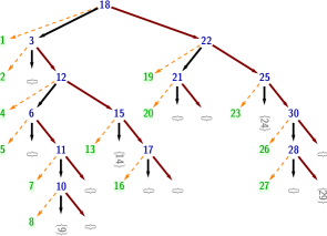
There is an intimate relation between jumplists and search trees, but the slight offset above complicates the matter.333The complication is inherent to the feature of jumplists that every key has at most one jump pointer. Skip lists, for example, can be transformed into BSTs directly [4]. Indeed, (random) jumplists are isomorphic to a rather peculiar variant of (random) BSTs (where random means “generated by insertions in random order”): the dangling-min BSTs (with leaf size ). Such a tree is defined for a sequence of (distinct) keys as follows. If , it is a leaf with the keys in sorted order. Otherwise, its root node contains two keys: the smallest key, , as its dangling min, and the first key of the sequence after the min has been removed as root key (i. e., the root key is , unless is the min; then it is ). The left resp. right subtrees of the root are the dangling-min BSTs for the keys smaller resp. larger than the root key in the remaining sequence (without root key and min, and preserving relative order). Dangling-min BSTs make the recursive decomposition in jumplists explicit, which helps for both designing algorithms and analyzing their performance.
We can transform a jumplist to a dangling-min BST (and vice versa): If , is a plain node and the dangling-min BST is a leaf containing all keys; (recall that a jumplist with nodes stores keys). Otherwise, is a jump node; with the key in and the key in , the root of the dangling-min BST has root key and dangling min . Next- resp. jump-sublist are recursively transformed into left and right subtree. Fig. 3 shows the jumplist corresponding to the given tree; Fig. 4 gives a larger example.
It is easy to see inductively that the dangling-min BST built from a randomized jumplist has the same distribution as if directly constructed for a random permutation of . We can therefore focus on analyzing the latter.
4 Spine Search
Searching a key in a jumplist is straightforward: We start at the header. We stop when the key in the current node is larger or equal to . Otherwise we follow either the jump pointer – if the key in is not larger than – or the next-pointer. We call this strategy the classic search in the sequel.444Brönnimann, Cazals, and Durand [2] also studied the symmetric alternative — compare first to and then with (if needed) — and found that it needs more comparisons on average.
However, there is an alternative search strategy not considered in [2] and [6], which performs better! Consider searching key in the jumplist from Fig. 1. A classic search in this list inspects keys in the given order; a total of key comparisons. Every step in the search that follows the next-pointer needs two comparisons.
Now do the search for in the dangling-min BST from Fig. 4, as if it was a regular BST (ignoring the subtree minima and stopping at the leaves). While doing so, we compare with keys . All these steps need only one key comparison even though mostly the same keys are visited as above. However, our search is not yet finished; the reached leaf contains only , and we would (erroneously!) announce that is not in the dictionary. Instead we have to return to the last node we entered through a right-child pointer and inspect all the dangling mins along the “left spine” of the corresponding subtree. In our example, we return to and make comparisons with and , terminating successfully. We call this search strategy spine search. In our example, it needed comparisons less than the classic search.
Spine search only compares with the dangling-mins for nodes on the left spine above the leaf, whereas the classic strategy does so for every node we leave through the left-child edge. Our modification is correct because when going to the right child we know that all keys left to are smaller than and thus cannot be any of the dangling minima we skipped. Appendix C gives detailed pseudocode.
The left spine is always a subset of the nodes where we took a left child edge, so spine search never needs more comparisons than the classic strategy. It seems reasonable that spine search should need roughly as many key comparisons as the search in a BST since most left spines are short. Indeed, we prove in § 7 that the linear search along the left spine is only a lower order term when averaging over all possible unsuccessful searches — spine search needs comparisons, compared to for the classic search strategy.
5 Median-of-k Jumplists
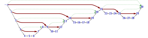
The search costs in BSTs can be improved by using medians of a small sample as subtree roots; the idea is called fringe-balancing in that context (§ 1.1) and corresponds to the median-of- rule for Quicksort [11, 5, 28]. Applied to our trees, we obtain -fringe-balanced dangling-min BSTs: if , we choose the root key as the median of the first keys in the sequence after removing the min (and otherwise proceed as before). Here is a fixed odd integer and we require .
Similarly, we define a randomized median-of- jumplist by choosing the jump target as the median of elements. The situation is illustrated below for and ; to have as the median of elements from the sample range, we must select further elements from and further elements from .
The number of such samples is , which we have to divide by the total number of possible samples, . The probability of a (legal) jump pointer configuration thus is
This puts more probability weight on balanced configurations, and hence improves the expected search costs. Fig. 5 shows a typical median-of- jumplist and its fringe-balanced dangling-min tree.555A possible generalization could use asymmetric sampling with and , where we select the st smallest instead of the median. Then, we have and in Equation (5). For the present work, we will however stick to the case .
Distribution of subproblem sizes
For our analysis, an alternative description of the distribution of the subproblem sizes is more convenient. Note that both and are always at least : the sublists must contain other sampled nodes plus their header. If we denote by , , we find that has a beta-binomial distribution (§ 2), . This implies that with , we have the mixed distribution conditional on .666The symmetry in the sublist sizes, , is a major convenience of our definition of jumplists as opposed to the original one.
6 Insert and Delete
The recursion structure for RestoreAfterDelete is similar.
We briefly sketch the update operations for randomized median-of- jumplists; Appendix C describes them in more detail. The common theme is that we first modify the jumplist blindly and afterwards “repair” the distribution by rebuilding one suitably chosen sublist randomly from scratch. For example upon insertion, the new node has a certain chance to be the target of the first jump pointer. We flip a coin to decide whether this should happen; if so, we rebuild the entire structure and are done. Otherwise, we recursively repair a sublist.
Rebalance
As in [2], we use a procedure Rebalance that (re)assigns jump pointers from scratch. It only uses the backbone, existing jump pointers are ignored. A careful recursive implementation of Rebalance rebuilds a sublist of nodes in time .
Insert
Insertion in jumplists consists of the three phases found in many dictionaries: (unsuccessful) search, local insertion, and cleanup. Unless is already present, the search ends at the node with the largest key (strictly) smaller than . There we insert a new node with key into the backbone.
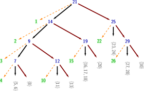
It does not have a jump pointer yet, and it is a new potential jump target for all the nodes whose sublist contains the new node. Procedure RestoreAfterInsert rectifies this as follows. Let be the total number of nodes after the insertion, i. e., including the new node. If , no cleanup is necessary; if , we draw the jump pointer for and are done. Otherwise, we first restore the pointer distribution of . Due to the insertion of a new node, the sample range now contains an additional node . ( is not necessarily the newly inserted node; if the new key is the first or second smallest in , is the former second node of ).
If we, conceptually, drew anew, there are two possibilities: either is part of the sample, namely with probability , or is not part of it. In the first case, we rebalance all of . In the second case, conditional on the event that is not in the sample, the current jump pointer of already has the correct distribution: the median of a random sample not containing . We thus rebalance with probability , where we draw the jump pointer of conditional on being part of the sample. Otherwise we continue recursively in the uniquely determined sublist that contains the inserted node. Fig. 6 summarizes RestoreAfterInsert graphically.
Delete
We now sketch the procedure RestoreAfterDelete, which is similar to RestoreAfterInsert. Let be the number of nodes after deletion, and let be the deleted node. First assume that . Assume , i. e., is a jump node whose sublist contained . If the sample drawn to choose did not contain , the deletion of does not affect , and we recursively clean up the sublist that formerly contained . If was part of the sample, we have to rebalance ; the probability for that is
(We define in case .) When the deleted node is , the new header can inherit ’s jump pointer and we have the same situation as if had been deleted. We have to rebalance with probability , otherwise we continue the cleanup in the next-sublist.
Cost Measure
Insertion and deletion consist of a search and RestoreAfterInsert/-Delete. The latter procedures retrace (a prefix of) the search path to the element and rebuild at most one sublist using Rebalance. So apart from the search costs (which we analyze separately), the dominating cost is the number of “rebalanced elements”: the size of the sublists on which Rebalance is called. We will use this as our measure of costs.
7 Analysis
We now turn to the analysis of the expected behavior of median-of- jumplists with leaf size . (The expectation is always over the random choices of the jump pointers.) We summarize our results in the theorem below. Its proof is spread over the following subsections.
Theorem 7.1:
Consider randomized median-of- jumplists with leaf size on keys, where and are fixed constants. Abbreviate by for the harmonic numbers. Then the following holds:
-
(a)
The expected number of key comparisons in a spine search is asymptotic to , as , when each position is equally likely to be requested.
-
(b)
The expected number of rebalanced elements in the cleanup after insertion is asymptotic to , as , when each of the possible gaps is equally likely.
-
(c)
The expected number of rebalanced elements in the cleanup after deletion is asymptotic to , as , when each key is equally likely to be deleted.
-
(d)
The expected number of additional machine words per key required to store the jumplist is asymptotically at most as .
7.1 Search Costs
Let be the (random) total number of comparisons to search all numbers (searching each gap once) in the randomized jumplist on , using SpineSearch. The corresponding quantity in BSTs is called external path length, and we will use this term for , as well. The quotient describes the average costs of one call to SpineSearch when all gaps are equally likely to be requested. is random w. r. t. to the locations of the jump pointers in . To set up a recurrence for , the perspective of random dangling-min BSTs is most convenient, since SpineSearch follows the tree structure. We describe recurrences here in terms of the distributions of families of random variables.
The terms and on the right-hand side denote members of independent copies of the family of random variables , which are also independent of , . (We omitted the superscripts above for readability.) Here , , and . (We use here instead of in § 5; hence the slightly different parameters.)
The terms in the expression for are the comparisons with (1) the root key, (2) the dangling min of the root, (3) the comparisons done in the left subtree while searching the leftmost gap (which does not exist in the subtrees any more!), and (4) the external path lengths of the subtrees. Two additional quantities are used to express these: is the number of keys in the leftmost leaf; by definition we have . is the number of internal nodes on the “left spine” of the tree, an essential parameter for the linear-search part of SpineSearch. is also the depth of the internal node with the smallest root key (ignoring dangling mins). For ordinary BSTs, is essentially the number of left-to-right minima, which is a well-understood parameter; for (fringe-balanced) dangling-min BSTs, such a simple correspondence does not seem to hold.
We point out that the distribution of has a subtle complication, namely that even conditional on , the quantities , and are not independent: all consider the same left subtree! For example, we always have (for ). We will only compute the expected value here, so by linearity, these dependencies can be ignored.
We will derive an asymptotic approximation using Thm. 2.5, the distributional master theorem (DMT).
Remark 7.1:
For ordinary BSTs, the expectation of above quantities is known precisely, and some generalizations for fringe-balanced trees are possible by solving an Euler differential equation for the generating function. Unlike there, for dangling-min BSTs the resulting differential equation is not an Euler equation. The case could be solved since the differential equation has order one [2], but there is little hope to obtain a solution for the generating function for .
Lemma 7.2:
.
breakProof 1
We apply Thm. 2.5 to the distributional recurrence . It has the form of (2) with (matching the notation of Thm. 2.5) . We have recursive term with size plus a “toll term” . The latter has the asymptotic form as , i. e., , , . Moreover, there is no “coefficient” in from of the recursive term, so .
We next check the conditions. The independence assumptions are trivially fulfilled here, in particular because is a fixed constant. We next consider (3). Recall that . By Lem. 2.2 and the remark below it, fulfills
for with . This function is a polynomial in , so it has bounded derivative (on the compact domain ) and is hence Lipschitz continuous (and thus Hölder continuous). So (3) is satisfied with . The limiting relative subproblem size has a distribution.
For the second condition, (4), we find that since is constant. So this condition is trivially satisfied with (which is a Hölder-continuous function). We have now established that we can apply the DMT to our recurrence.
To obtain the asymptotic approximation for , we consider , so Case 2 applies: for the constant . (Note that this constant only involved the limiting relative subproblem size , not the relative subproblem size for a fixed .) The expectation in is exactly the first part of Lem. 2.4, so we find . Now the claim follows by inserting above.
Remark 7.2 (Spine lengths):
Lem. 7.2 implies that the expected left spine of the root is logarithmic – as one might expect in a random BST; indeed, the expected left spine lengths of the root in a random BST and a dangling-min BST differ only in lower order terms. Note that the former is exactly and the proof is elementary: The left spine length in a BST is the number of left-to-right minima in the insertion order. For dangling-min BSTs, no such simple argument is available.
With these preparations, we can prove the main statement about search costs.
breakProof 2 break(Thm. 7.1–(a))
We again use the distributional master theorem (DMT); this time on the recurrence . The recurrence is more involved than the one for that we just solved, but the distribution of subproblem sizes are the same, and we again have no coefficient in front of the recursive terms. Therefore, a large part of the argument can be copied from the proof of Lem. 7.2.
We here have , there are recursive terms and . By Lem. 7.2, all but the first summand in are actually in , so from the initially complicated toll function, only remains in the leading term as . We thus have , , .
7.2 Insertion Costs
The steps taken by RestoreAfterInsert depend on the position of the newly inserted element; we denote here by the rank of the gap the new element is inserted into. When the current sublist has nodes, we have . Similar as for searches, we consider the average costs of insertion when all possible gaps are equally likely to be requested.
Unlike for searches, the distribution of in subproblems is not uniform even when is: a close inspection of RestoreAfterInsert reveals that (a) recursive calls in the jump-sublist always have , and (b) and yield in the recursive call in the next-sublist; in fact, once holds, we get this rank in all later recursive calls. We can therefore handle this by splitting the cases and ; Also note that for the topmost call to RestoreAfterInsert, is not possible, since no insertion before the header with dummy-key is possible. This means that initially holds. Recall that a jumplist on nodes stores only keys, so that there are only possible gaps. We obtain the following distributional recurrence for , the random number of rebalanced elements during insertion into the th gap in a randomized median-of- jumplist with nodes. (Note that unlike in the pseudocode, is here the number of nodes in the jumplist before the insertion.)
All terms on the right-hand side denote independent copies of the family of random variables and and are independent of and . Here , , and (as in § 5).
Lemma 7.3:
.
breakProof 3
We use once more the distributional master theorem. As before, and the condition (3) is satisfied by Lem. 2.2. We have . Unlike before, we here have a non-constant coefficient in front of the recursive term, but since , (4) is again fulfilled with . As in the proof of Lem. 7.2, we find (Case 2) and with the claim follows from (Lem. 2.4).
breakProof 4 break(Thm. 7.1–(b))
7.3 Deletion Costs
As for insertion, we analyze the size of the sublist that is rebuilt using Rebalance when the rank of the deleted element is chosen uniformly. Initially, we have since the dummy key in the header cannot be deleted. In recursive calls, also is possible, and we remain in this case for good whenever we enter it once. We can thus characterize the deletion costs using the two quantities and . As for insertion, is the “old” size of the jumplist, i. e., the number of nodes before the deletion.
As before, the terms on the right are independent copies of the family of random variables and and / are independent of and . We have , , and . The (asymptotic) solution of these recurrences is similar to the case of insertion, but a few more complications arise.
Lemma 7.4:
For we have . If , .
breakProof 5
For , we have (almost surely) in each iteration, so the recurrence collapses to its initial condition, which is at most . In the following, we now consider . The proof will ultimately use the DMT on , but we need a few preliminary results to compute the toll function . We write the to mean here and throughout. With that notation, we give the following elementary approximation:
| (5) |
Now, we compute the expectation of conditional on .
Next, we use the stochastic representation of beta-binomials (recall § 2); we take expectations over with , but conditional on . We write . Then it holds that
Finally, we also compute the expectation w. r. t. ; note that for , exists and has a finite value (independent of ); whereas for , the error term is zero. So we find in both cases with Lem. 2.1:
| (6) |
With this we finally get . and fulfills (3). For (4), we compute
So the DMT applies; we have , i. e., Case 2. The claim follows with .
breakProof 6 break(Thm. 7.1–(c))
7.4 Memory Requirements
We assume that a pointer requires one word of storage, and so does an integer that can take values in . We do not count memory to store the keys since any (general-purpose) data structure has to store them. This means that a plain node requires word of (additional) storage, and a jump node needs additional words (two pointers and one integer). Let denote the (random) number of jump nodes, excluding the dummy header, of a random median-of- jumplist with leaf size on keys, then its additional memory requirement is . It remains to show that is asymptotically at most .
counts the internal nodes in a random fringe-balanced dangling-min BST over keys; a distributional recurrence is thus easy to set up:
Here again , , and . For , the DMT only gives us (Case 3). It is easy to see that is also , but a precise leading-term seems very hard to obtain.
breakProof 7 break(Thm. 7.1–(d))
The recurrence for is very similar to that for the number of partitioning steps in median-of- Quicksort with Insertionsort threshold ; the only difference is that we there have , i. e., with instead of . By monotonicity, is at most the number of partitioning steps in Quicksort since also the subproblems sizes are smaller. The number of partitioning steps in median-of- Quicksort with Insertionsort threshold is , see, e. g., [10, p. 327]. Setting yields the claim.
8 Conclusion
In this article, we presented median-of- jumplists and analyzed their efficiency in terms of the expected number of comparisons (for searches) and rebalanced elements (for updates). The precise analysis of insertion and deletion costs is also novel for the original version of jumplists ().
Our analysis shows that a search profits from sampling; in particular going from to entails significant savings: instead of comparisons on average. As for median-of- Quicksort, we see diminishing returns for much larger . For jumplists, also the cleanup after insertions and deletions gets more expensive; the effort grows linearly with . Very large will thus be harmful.
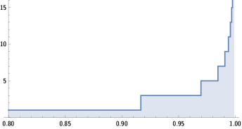
The efficiency of insertion and deletion depends on both the time for search and the time for cleanup, so it is natural to ask for optimal . Since the cost units are rather different (comparisons vs. rebalanced elements) we need a weighing factor. Depending on the relative weight of comparisons, we can compute optimal , see Fig. 7. In the realistic range, we should try , , or , unless we do many more searches than updates.
We conducted a small running time study based on a proof-of-concept implementation [27] in Java that confirms our analytical findings: Sampling leads to some savings for searches, but slows down insertions and deletions significantly. Comparing running times with that of Java’s TreeMap (a red-black tree implementation) shows that our data structure is only partially competitive: for iterating over all elements, jumplists are about 50% faster, but searches are between 20% and 100% slower (depending on the choice for ) and for insertions/deletions TreeMaps are 5 to 10 times faster. However, TreeMaps use 4 additional words per key (without even storing subtree sizes needed for efficient rank-based access), whereas our jumplists never need more than additional words per key and less than with . For keys, did not affect searches much () but actually sped up insertions and deletions (roughly by a factor of 2!).
8.1 Future Work
Some interesting questions are left open. What is the optimal choice for ? Answering this question requires second-order terms of search, insertion and deletion costs; due to the underlying mathematical challenges it is unlikely that those can be computed exactly, but an upper bound using analysis results on Quicksort should be possible. Other future directions are the analysis of branch misses, in particular in the context of an asymmetric sampling strategy, and the design of a “bulk insert” algorithm that is faster than inserting elements subsequently, one at a time.
On modern computers the cache performance of data structures is important for their running time efficiency. Here, a larger fanout of nodes is beneficial since it reduces the expected number of I/Os. For jumplists this can be achieved by using more than one jump pointer in each node. The case of two jump pointers per node has been worked out in detail [18], but the general scheme invites further investigation.
Appendix
.0.0\EdefEscapeHexAppendixAppendix\hyper@anchorstart.0\hyper@anchorend \manualmark\markleftMedian-of- Jumplists and Dangling-Min BSTs
Appendix A Index of Notation
In this appendix, we collect the notations used in this work.
A.1 Generic Mathematical Notation
-
, , , , .
natural numbers , , integers , rational numbers , real numbers .
-
, etc. .
restricted sets .
-
.
repeating decimal; ;
numerals under the line form the repeated part of the decimal number. -
, .
natural and binary logarithm; , .
-
.
to emphasize that is a random variable it is Capitalized.
-
.
real intervals, the end points with round parentheses are excluded, those with square brackets are included.
-
, .
integer intervals, ; .
-
, .
Iverson bracket, if stmt is true, otherwise.
-
.
th harmonic number; .
-
, , , ,
.
asymptotic notation as defined, e. g., by [7, Section A.2]; is equivalent to .
-
.
with absolute error ; formally the interval ; as with -terms, we use “one-way equalities”: instead of .
-
.
the gamma function, .
-
.
the digamma function, .
-
.
the beta function,
-
, .
factorial powers notation of Graham et al. [8]; “ to the falling resp. rising.”
-
.
the binary base- entropy function .
A.2 Stochastics-related Notation
-
, .
probability of an event resp. probability for random variable to attain value .
-
.
expected value of .
-
.
equality in distribution; and have the same distribution.
-
, .
indicator variable for event , i. e., is if occurs and otherwise; denotes the event induced by the expression .
-
.
Bernoulli distributed random variable; .
-
.
uniformly in distributed random variable.
-
.
discrete uniformly in distributed random variable.
-
.
beta distributed random variable with shape parameters and .
-
.
binomial distributed random variable with trials and success probability ; . is equivalent to .
-
.
beta-binomial distributed random variable; , ; is equivalent to .
A.3 Notation for Jumplists and Analysis
-
, .
sample size , ; jump pointers are chosen as median of elements.
-
.
leaf size; (sub)lists with (equivalently: ) do not use jump pointers.
-
.
number of keys stored; the input size.
-
, .
the number of nodes; (the header does not store a key).
-
.
the stored keys; .
-
.
the nodes of a jumplist on keys, in the order of the backbone, i. e., and , .
-
.
random jumplist on keys ; obtained from Rebalance on a list with keys .
-
sublist of node .
the sublist that starts at (inclusive) and extends up to (excluding) the first node targeted by a jump pointer of a node with or up to (including) the end of the whole list if not such pointer exists.
-
, .
the next-sublist (of a given node ); the sublist of ; (only defined for jump nodes).
-
, .
the jump-sublist (of a given node ); the sublist of . (only defined for jump nodes).
-
, .
(random) sublist sizes; is the number of nodes in , ; ;
-
, .
.
Appendix B Comparison of Jumplist Definitions
Our definition of jumplists differs in some details from the original version. We list the differences here, and discuss why we think that our modifications are appropriate.
Symmetry
In the original version of the jumplist, the jump pointer is allowed to target any node from the sublist, except the header itself. Thus there are possible choices. In this setting, the size of the next-sublist can attain any value between and , whereas the size of the jump-sublist is between and .
We disallow the direct successor of the head as possible target. This modification restores symmetry between next- and jump-sublist: both must be non-empty and contain at most nodes and their sizes have the same distribution. Moreover, forbidding the direct successor as jump target is also a natural requirement since such a degenerate “shortcut” is useless in searches.
Small Sublists
The original jumplists only have one type of nodes which corresponds to our jump node. In the case , Brönnimann, Cazals, and Durand resort to assigning an “exceptional pointer” to the direct successor; note that this node actually lies outside (one behind) of the current sublist. These pointers are of no use, as they are never followed during (jump-and-walk) search.
In implementations with heap-allocated memory for each node, it is often not a problem to have different node types (and sizes), and it potentially allows to save memory. We thus introduced the plain node without jump pointer, used whenever the sublist has at most nodes. is required if we want to avoid useless jump pointers that point to the direct successor.
This also allows us enforce that every node has at most one incoming jump pointer; this is another natural requirement from the perspective of a search starting at the header: shortcuts with the same target are redundant. The parameter allows us to trade space for time.
Sentinel vs. Circularly closed
The original jumplist implementation has a circularly closed backbone, i. e., the next pointer of the last node in the list points to the overall header again, avoiding special treatment for an empty list. Since the backbone is sorted, we can instead add a sentinel node with key at the end of the list, so we can omit any explicit boundary checks during searches.
Appendix C Algorithms
In this appendix, we give the more details the insertion and deletion algorithms for randomized median-of- jumplists.
We describe the procedures in prose and an intuitive graphic syntax, as well as in detailed pseudocode; see § C.4 for the latter. We also point out that our proof-of-concept implementation in Java is available online for interested readers [27].
As a simple example to introduce the graphical syntax, here is the transformation from jumplists to dangling-min BSTs pictorially:
The first equation defines minBST on small jumplists (); it shows a header without jump pointer, i. e., a plain node. The second equation defines minBST on larger jumplists. Whenever variables appear on the left side, they are understood as formal placeholders of a pattern to be matched against the actual input. This mimics the corresponding feature of many functional programming languages that allows to define a function case by case in this syntax. The parts that match the variables are then used on the right-hand side.
Graphical syntax conventions
We now proceed to the description of the insertion and deletion procedures. We use the following conventions: The input of the algorithms, the “old” jumplist, is drawn as rectangle (or abbreviated by ). A sequence of (output) leaf nodes is depicted by a rectangle with rounded corners. The position of insertion resp. deletion is marked in red. If the algorithm makes a random choice, each outcome is multiplied with its probability, and all outcomes are added up.
C.1 Rebalance
Algorithm Rebalance is used if a jumplist needs to be (re)built from scratch. It only uses the backbone of the argument, any existing jump pointers are ignored. In the base case, i. e., if the argument contains nodes, a linked list of plain nodes with the same keys is returned.
If contains nodes, must become a jump node and we have to draw a jump target from the sample range. Conceptually, a sample of nodes is drawn and the median w. r. t. the keys is chosen. The same distribution can actually be achieved without explicitly drawing samples using a random variable (see § 5). Then the node is the jump target. After the jump pointer of has been initialized, the resulting next- and jump-sublist are rebalanced recursively.
C.2 Insert
Insert in jumplists consists of three phases found in many tree-based dictionaries: (unsuccessful) search, insertion, and cleanup. Unless is already present, the search ends at the node with the largest key (strictly) smaller than . There we insert a new node with key into the backbone.
The new node however does not have a jump pointer yet. Furthermore, the new node might need to be considered as potential jump target of its predecessors in the backbone. Thus, for all the nodes that have the new node in their sublist, we need to restore the pointer distribution. This is carried out by RestoreAfterInsert.
Let be the number of nodes after the insertion, i. e., including the new node. If , the new node remains a plain node within a list of plain nodes, and no cleanup is necessary. If due to the insertion, , which was a plain node before, now has to become a jump node. In this case, Rebalance is called on and the insertion terminates.
If , we first restore the pointer distribution of . Due to the insertion of a new node, the sample range now contains an additional node . Note that is not necessarily the newly inserted node; if the new key is the first or second smallest in , is the former second node of .
If we, conceptually, wanted to draw pointers for anew, there are two possibilities: either is part of the sample, or is not part of the sample. The probability for the latter case is
| (C.1) |
since the overall number of -samples from items is and if we forbid, say, item , we have choices left.
Let us denote by the counter probability, i. e., the probability that is part of the sample. In that case, we have to rebalance all of . Conditional on the event that is not in the sample, the existing jump pointer of has the correct distribution: it has been chosen as the median of a random sample not containing .
In the algorithm, we thus rebalance with probability , where we draw the jump pointer of conditional on being part of the sample. Otherwise, ’s jump pointer can be kept, and we continue recursively in the uniquely determined sublist that contains the inserted node — that is, unless does not have a jump pointer yet, since is the newly inserted node. In that case, we simply steal the jump pointer of its direct successor, , which has the correct conditional distribution. Now does not have a jump pointer, and we treat this case recursively, as if was the newly inserted node.
C.3 Delete
Delete has the same three phases as Insert: first a (successful) search finds the node to be deleted, then we actually remove it from the backbone. Finally, RestoreAfterDeletion performs the cleanup: the pointer distribution for those nodes whose sublists contained the deleted node has to be restored since their sample range has shrunk.
Let be the number of nodes after deletion, and let be the deleted node. We first assume that ; the case of deleting will be addressed later. If , is a list of plain nodes and can remain unaltered. If , the size dropped from to due to the deletion, so has to be made a plain node.
Otherwise (), is a jump node whose sublist contained . There are two possible cases: either the sample drawn to choose contained , or not. In the latter case, the deletion of does not affect the choice for at all, and we recursively cleanup the uniquely determined sublist that formerly contained . If was indeed part of the sample, we have to rebalance .
It remains to determine the probability that was in the sample that led to the choice of . Unlike for insertion, now depends on these two nodes. Let resp. be the sizes of the next- resp. jump-sublist before deletion; recall that we store in . Then is given by the following expression:
| (C.2) |
The correctness is best seen in a case-by-case argument, which we give below. But before we do that, we have to consider the case that the deleted node is . Then has become the new header, but its jump pointer now has the wrong distribution since ’s jump pointer no longer delimits its sample range. But observe that ’s (old) sample range was exactly ’s new sample range plus . Accordingly we only have to rebalance in case was part of the sample to select , which happens with probability . Otherwise, we can conceptually impose ’s jump pointer on , which is easily implemented by swapping their keys, and continue the cleanup recursively in the next-sublist, as if had been deleted.
Overall, the following situations can occur upon deletion:
-
1.
If the jump pointer of targeted the deleted node, the whole list is re-built with probability .
-
2.
If no sampling is used, i. e., , the list only needs to be reconstructed in the following two cases:
-
(a)
If the deleted node had rank and next-size , we cannot impose the jump pointer of the deleted node onto as the target is not valid. Thus the list is reconstructed.
-
(b)
If the deleted node had rank and had next-size , the only node in the next-sublist has been deleted. This results in an invalid pointer configuration, therefore the list is reconstructed.
-
(a)
-
3.
If the deleted node was contained in the next-sublist of , i. e., , it was part of the sample with probability
-
4.
If the deleted node was contained in the jump-sublist of , it was part of the sample with probability .
To conclude, depending on the outcome of the coin flip, the algorithm either rebalances the current sublist (with probability ) (as given above) and terminates, or it reuses the topmost old jump pointer and continues recursively.
C.4 Pseudocode
We give full pseudocode for all basic operations on median-of- jumplists with leaf size in this section.
We first list the four procedures Contains, Insert, Delete and RankSelect that constitute the public interface of the data structure; the other procedures can be thought of as low-level procedures typically hidden from the user of the data structure.
We assume that jumplists are represented using the following records/objects.
-
Used Objects/Structs
References/pointers to nodes can refer to a PlainNode or to a JumpNode, and we assume there is an efficient method to check which type a particular instance has. If is a reference to a PlainNode, we write and for the key-value and next-pointer fields of the referenced PlainNode; similarly for the other types.
-
// Returns whether is present in and how many elements it stores. return
-
// Insert into ; does nothing if is already present. if // not yet present // Add new node in backbone. ; end if
-
// Removes from ; does nothing if is not present. if // is present // Remove from backbone. ; end if
-
// Returns the element with (zero-based) rank , i. e., the st smallest element. ; repeat if ; else ; end if if then return end if until is PlainNode repeat ; until return
The above methods make use of the following internal procedures. We give a spine search implementation that is augmented to determine also the rank of the found element. Using the rank makes the procedures to restore the distribution after insertions or deletions a bit more convenient to state, and also avoids re-doing key comparisons there.
The given implementation of SpineSearch, Contains, Insert, and Delete assume a sentinel node at the end of the linked list that has , i. e., a value larger than any actual key value; we do however not count towards the nodes of a jumplist since can be shared across all instances of jumplists. The sentinel may never be the target of any jump pointer. We could avoid the need for the sentinel at the expense of a null-check of the next pointer, before comparing the successor’s key (line C.4 in SpineSearch, line C.4 in Contains, line C.4 in Insert, and line C.4 in Delete). Since using the sentinel is a bit more efficient and gives more readable code, we stick to this assumption.
-
// Returns last node with key and its zero-based rank, // i. e., the number of nodes with key ; ; repeat // BST-style search if ; else ; end if until is PlainNode while // Linear search from ; end while return
-
// Draws jump pointers in for nodes starting with (inclusive) // according to the randomized jumplist distribution. // Returns new first (possibly still ) and last node of the sublist. if Replace and its successors by linked PlainNodes. return else random -element subset of // in general return end if
-
// Rebalances the sublist starting at containing nodes, // where we fix the topmost jump pointer to point to the element of rank . // Returns new first (possibly still ) and last node of the sublist. return
-
// Restore distribution in sublist with header and of size after an insertion at position . // is the number of nodes in the sublist, including the new element // Returns the new head of the sublist (possibly still ). if // Base case if // We need a new JumpNode, so rebalance. end if else // with probability if // Rebalance conditional on new index being in sample. random -element subset of // in general else // topmost jump pointer can be kept if // new node is head of sublist, so steal successor’s jump. // Swap roles of the two nodes. Swap and fields of and . end if if // New element is in next-sublist. ; else // New element is in jump-sublist. if // Have to reconnect backbone end if end if end if end if return
-
// Restore distribution in sublist with header and size after a deletion at position . // is the number of nodes in the sublist, excluding the just deleted element . // Returns the new head of the sublist (possibly still ). if if // head is a JumpNode, must become PlainNode end if else // with probability if // Rebalance sublist. else // Topmost jump pointer can be kept. if // Impose deleted head’s pointer onto successor. // Swap roles of the two nodes. Swap and fields of and . Swap and . end if if // Deletion in next-sublist. ; else // Deletion in jump-sublist. if // Have to reconnect backbone end if end if end if end if return
Appendix D Omitted proofs
breakProof 8 break(Lem. 2.3)
For , we compute
For the first part of the claim, we set and find that the sum reduces to ; for the second part of the claim, we use and note that the expression in the outer parentheses is at most .
breakProof 9 break(Lem. 2.4)
We use the following known integral; see [26, Eq. (2.30)]:
| (D.1) |
Here is the digamma function. Then we find
and
References
- [1] A. Andersson, R. Fagerberg, and K.S. Larsen. Balanced binary search trees. In D. Mehta and S. Sahni, editors, Handbook of Data Structures and Applications, chapter 10. CRC Press, 2005.
- [2] Hervé Brönnimann, Frédéric Cazals, and Marianne Durand. Randomized jumplists: A jump-and-walk dictionary data structure. In STACS 2003, pages 283–294, 2003. doi:10.1007/3-540-36494-3_26.
- [3] R. Casas, J. Díaz, and C. Martinez. Statistics on random trees. In International Colloquium on Automata, Languages, and Programming (ICALP), pages 186–203. Springer, 1991. doi:10.1007/3-540-54233-7_134.
- [4] Brian C. Dean and Zachary H. Jones. Exploring the duality between skip lists and binary search trees. In Annual southeast regional conference, pages 395–399. ACM Press, 2007. doi:10.1145/1233341.1233413.
- [5] Michael Drmota. Random Trees. Springer, 2009.
- [6] Amr Elmasry. Deterministic jumplists. Nordic Journal of Computing, 12(1):27–39, 2005.
- [7] Philippe Flajolet and Robert Sedgewick. Analytic Combinatorics. Cambridge University Press, 2009. URL: http://algo.inria.fr/flajolet/Publications/book.pdf.
- [8] Ronald L. Graham, Donald E. Knuth, and Oren Patashnik. Concrete Mathematics: A Foundation For Computer Science. Addison-Wesley, 1994.
- [9] Daniel Hill Greene. Labelled formal languages and their uses. Ph. D. thesis, Stanford University, 1983.
- [10] Pascal Hennequin. Combinatorial analysis of Quicksort algorithm. RAIRO - Theoretical Informatics and Applications, 23(3):317–333, 1989.
- [11] Pascal Hennequin. Analyse en moyenne d’algorithmes : tri rapide et arbres de recherche. Thèse (Ph. D. Thesis), Ecole Politechnique, Palaiseau, 1991.
- [12] Shou-Hsuan Stephen Huang and C. K. Wong. Binary search trees with limited rotation. BIT, (4):436–455, 1983. doi:10.1007/BF01933619.
- [13] Shou-Hsuan Stephen Huang and C. K. Wong. Average number of rotations and access cost in iR-trees. BIT, 24(3):387–390, 1984. doi:10.1007/BF02136039.
- [14] Donald E. Knuth. The Art Of Computer Programming: Searching and Sorting. Addison Wesley, 2nd edition, 1998.
- [15] Hosam M. Mahmoud. Evolution of Random Search Trees. Wiley, 1992.
- [16] Conrado Martínez and Salvador Roura. Randomized binary search trees. J. ACM, 45(2):288–323, 1998. doi:10.1145/274787.274812.
- [17] J. Ian Munro, Thomas Papadakis, and Robert Sedgewick. Deterministic skip lists. In ACM-SIAM Symposium on Discrete Algorithms, SODA 1992, pages 367–375. SIAM, 1992.
- [18] Elisabeth Neumann. Randomized Jumplists With Several Jump Pointers. Bachelor’s thesis, 2015. URL: http://nbn-resolving.de/urn/resolver.pl?urn:nbn:de:hbz:386-kluedo-41642.
- [19] J. Nievergelt and E. M. Reingold. Binary search trees of bounded balance. SIAM Journal on Computing, 2(1):33–43, 1973. doi:10.1137/0202005.
- [20] Tomi A. Pasanen. Random binary search tree with equal elements. Theoretical Computer Science, 411(43):3867–3872, 2010. doi:10.1016/j.tcs.2010.06.023.
- [21] Patricio V Poblete and J. Ian Munro. The analysis of a fringe heuristic for binary search trees. Journal of Algorithms, 6(3):336–350, 1985. doi:10.1016/0196-6774(85)90003-3.
- [22] William Pugh. Skip lists: A probabilistic alternative to balanced trees. Communications of the ACM, 33(6):668–676, 1990. doi:10.1145/78973.78977.
- [23] Salvador Roura. Improved Master Theorems for Divide-and-Conquer Recurrences. Journal of the ACM, 48(2):170–205, 2001.
- [24] R. Seidel and C. R. Aragon. Randomized search trees. Algorithmica, 16(4-5):464–497, 1996. URL: http://link.springer.com/10.1007/BF01940876, doi:10.1007/BF01940876.
- [25] A. Walker and D. Wood. Locally balanced binary trees. The Computer Journal, 19(4):322–325, 1976. doi:10.1093/comjnl/19.4.322.
- [26] Sebastian Wild. Dual-Pivot Quicksort and Beyond: Analysis of Multiway Partitioning and Its Practical Potential. Doktorarbeit (Ph. D. thesis), Technische Universität Kaiserslautern, 2016. URL: http://nbn-resolving.de/urn/resolver.pl?urn:nbn:de:hbz:386-kluedo-44682.
- [27] Sebastian Wild. sebawild/jumplists: snapshot-for-paper. 2016. doi:10.5281/zenodo.155326.
- [28] Sebastian Wild. Quicksort is optimal for many equal keys. In Workshop on Analytic Algorithmics and Combinatorics (ANALCO), pages 8–22. SIAM, 2018. doi:10.1137/1.9781611975062.2.