The inner mass distribution of late-type spiral galaxies from SAURON stellar kinematic maps

Abstract

We infer the central mass distributions within 0.4–1.2 disc scale lengths of 18 late-type spiral galaxies using two different dynamical modelling approaches – the Asymmetric Drift Correction (ADC) and axisymmetric Jeans Anisotropic Multi-gaussian expansion (JAM) model. ADC adopts a thin disc assumption, whereas JAM does a full line-of-sight velocity integration. We use stellar kinematics maps obtained with the integral-field spectrograph SAURON to derive the corresponding circular velocity curves from the two models. To find their best-fit values, we apply Markov Chain Monte Carlo (MCMC) method. ADC and JAM modelling approaches are consistent within 5% uncertainty when the ordered motions are significant comparable to the random motions, i.e, $\overline{v_{\phi}}/\sigma_{R}$ is locally greater than 1.5. Below this value, the ratio $v_{\mathrm{c,JAM}}/v_{\mathrm{c,ADC}}$ gradually increases with decreasing $\overline{v_{\phi}}/\sigma_{R}$, reaching $v_{\mathrm{c,JAM}}\approx 2\times v_{\mathrm{c,ADC}}$. Such conditions indicate that the stellar masses of the galaxies in our sample are not confined to their disk planes and likely have a non-negligible contribution from their bulges and thick disks.

1 Introduction

The non-Keplerian rotation curves of spiral galaxies provided the first observational evidence that galaxies are embedded in extensive dark matter haloes (Bosma 1978; Rubin & Ford 1983; van Albada et al. 1985; Begeman 1987). Historically, the 21-cm emission from atomic neutral hydrogen gas (HI) has been the main tool to derive galaxy rotation curves, because of its capability to trace the gravitational field beyond the optical stellar disc. However, HI is less useful in constraining the rotation curve in the central parts of discs usually due to insufficient spatial resolution and the lack of HI gas in the inner parts of galaxies (e.g., Noordermeer et al. 2007). The interstellar medium in the centre is instead dominated by gas in the molecular and ionised phases (e.g., Leroy et al. 2008). Unfortunately, the rotation curves derived through CO emission, the common tracer for the molecular gas distribution, often show non-axisymmetric signatures such as wiggles (Wada & Koda 2004; Colombo et al. 2014). Hot ionised gas has the additional disadvantage that the observed rotation alone is often insufficient to trace the total mass distribution and that its velocity dispersion needs to be included. This velocity dispersion is generally influenced by a typically unknown contribution from non-gravitational effects such as stellar winds and shocks (e.g., Weijmans et al. 2008).

Some of these shortcomings of gas tracers can be overcome through careful correction and analysis. However, a broader shortcoming of gas tracers becomes apparent because of their dissipative nature. The gas is easily disturbed by perturbations in the plane from, for example, a bar or spiral arm (Englmaier & Gerhard 1999; Weiner, Sellwood & Williams 2001; Kranz, Slyz & Rix 2003). Gas also settles in the galaxy disc plane (or polar plane) and is thus less sensitive to the mass distribution perpendicular to it. The typical velocity dispersions of the neutral and ionized gas, respectively, are $\sim$10 km s^-1(Casertano 1983; Caldú-Primo et al. 2013) and $\sim$20 km s^-1(e.g. Fathi et al. 2007).

Instead of gas, stars could be used as a tracer of the underlying gravitational potential. Stars are present in all galaxy types, are distributed in all three dimensions, and are collisionless making them less susceptible to perturbations. The random motion of the collisionless stars tipycally ranges from 20 km s^-1to above 300 km s^-1(Dehnen & Binney 1998; Martinsson et al. 2013a; Cappellari et al. 2013; Ryś, Falcón-Barroso & van de Ven 2013; Ganda et al. 2006). This implies a scale height difference of over an order of magnitude between the gaseous and stellar components (e.g., Koyama & Ostriker 2009; Bottema 1993).

However, we need to measure both the ordered and random motions of stars before they can be used as a dynamical tracer. Their random motion can be different in all three directions, an effect known as the velocity anisotropy. This anisotropy requires more challenging observational and modelling techniques to uncover the total mass distribution. Nonetheless, these techniques are becoming available. Integral-field spectrographs like SAURON (Bacon et al. 2001), which is used in this study, allow us to extract high-quality stellar kinematic maps and enable us to perform dynamical models.

A common approach for spiral galaxies is to apply the asymmetric drift correction (ADC; Binney & Tremaine 2008) to infer the circular velocity curve from the measured stellar mean velocity and velocity dispersion profiles. This approach is straightforward since the velocity and dispersion profiles can be obtained from long-slit spectroscopy, and no line-of-sight integration is required due to an underlying thin-disc assumption. Using this method requires assuming both the disc inclination and the magnitude of the velocity anisotropy. As such, the ADC approach is widely adopted in studies that use the stellar kinematics to infer the circular velocity curve. For example, when investigating the Tully-Fisher relation for earlier-type spirals (e.g., Bottema 1993, Neistein et al. 1999; Williams, Bureau & Cappellari 2010), the speed of bars (e.g., Aguerri, Beckman & Prieto 1998; Buta & Zhang 2009), as well as the inner distribution of dark matter (e.g., Kregel, van der Kruit & Freeman 2005; Weijmans et al. 2008).

In this paper, we adopt an alternative approach, namely fitting a solution of the axisymmetric Jeans equations to stellar mean velocity and velocity dispersion fields to infer mass distributions. We apply this approach to the data acquired with the integral-field spectrograph SAURON from inner parts of 18 late-type Sb–Sd spiral galaxies. These Jeans models are less general than orbit-based models (e.g., Schwarzschild’s method; van den Bosch et al. 2008) but are far less computationally expensive while still providing a good description of galaxies dominated by stars on disc-like orbits (e.g., Cappellari 2008). The applicability of these fitted Jeans solutions even applies to dynamically hot systems such as lenticular galaxies. The Jeans models take into account the two-dimensional information in the stellar kinematic maps as well as integration along the line-of-sight. We also compare the resulting circular velocity curves with those obtained through ADC to investigate the validity of the assumptions underlying the simpler ADC approach.

In Section 2, we summarise the sample including the SAURON observations and near-infrared imaging. The Jeans and ADC modelling approaches are described in Section 3 and applied via Markov Chain Monte Carlo technique in Section 4. We then compare the circular velocity curves from both modelling approaches in Section 5 and discuss the possible reasons for the significant differences we find in Section 6. We draw our conclusions in Section 7.

2 Observations

Table 1: Properties of our sample of 18 galaxies (see Sec. 2.1): (1) Galaxy identifier; (2) Hubble type (G06 from NED); (3) Galactocentric distance in Mpc (G06 from NED); (4) Photometric position angle in degrees from DSS images with a typical uncertainty from 5^∘to 10^∘ (G09; Sec. 2.1 ) ; (5) Ellipticity from DSS images with a typical uncertainty of 15 ^∘ (G09; Sec. 2.1 ); (6) Adopted inclination in ADC and JAM approaches, where the values marked with star correspond to the minimum allowed inclinations in JAM model (see Sec. 2.1); (7) Systemic velocity in km s^-1, measured using the enforced point-symmetry method with typical uncertainty of 1 km s^-1 (Sec. 4.2); (8) Galaxy MGE effective radius in arcseconds with a typical uncertainty of 10% (Sec. 2.1); (9) Radial extent of the stellar kinematic data in arcseconds with a typical uncertainty of 1% (Sec. 2.1); (10) Disk scale length in arcseconds with a typical uncertainty of 5% (G09); (11) Effective radius of the bulge in arcseconds with a typical uncertainty of 15% (G09); (12) Radial extent of the stellar kinematic data in terms of disk scale lengths with a typical uncertainty of 5% (Sec. 2.1)

NGC	Type	D	PA	$\epsilon$	i	$V_{\mathrm{sys}}$	$R_{e}$	$R_{\mathrm{max}}$	$h_{d}$	$r_{b}$	$(\frac{R_{\mathrm{max}}}{h_{d}})$
(1)	(2)	(3)	(4)	(5)	(6)	(7)	(8)	(9)	(10)	(11)	(12)
0488	SA(r)b	32.1	5	0.230	42	2299	53.6	19.2	42.7	9.9	0.4
0772	SA(s)b	35.6	126	0.340	51	2506	54.0	20.6	47.1	19.0	0.4
4102	SAB(s)b	15.5	42	0.445	59	838	15.0	22.1	19.5	1.5	1.1
5678	SAB(rs)b	31.3	5	0.475	61	1896	24.4	24.0	20.9	3.1	1.1
3949	SA(s)bc	14.6	122	0.360	53	808	20.4	22.1	16.8	4.6	1.3
4030	SA(s)bc	21.1	37	0.240	43	1443	30.2	19.2	26.5	15.3	0.7
2964	SAB(r)bc	20.6	96	0.450	59	1324	20.8	21.0	16.9	1.0	1.2
0628	SA(s)c	9.8	25	0.190	38	703	90.7	22.1	70.7	12.3	0.3
0864	SAB(rs)c	21.8	26	0.320	50	1606	38.3	15.1	28.1	1.6	0.5
4254	SA(s)c	19.4	50	0.270	46	2384	52.1	19.2	40.7	15.8	0.5
1042	SAB(rs)cd	18.1	174	0.290	47	1404	73.4	15.1	52.5	4.4	0.3
3346	SB(rs)cd	18.9	100	0.160	42⋆	1257	55.3	17.8	35.4	3.2	0.5
3423	SA(s)cd	14.7	41	0.230	42	1001	52.6	20.1	40.1	9.7	0.5
4487	SAB(rs)cd	14.7	77	0.370	53	1016	49.8	19.2	36.8	10.6	0.5
2805	SAB(rs)d	28.2	125	0.240	43	1742	65.8	12.6	50.8	13.0	0.3
4775	SA(s)d	22.5	96	0.135	34⋆	1547	29.0	17.8	19.3	8.3	0.9
5585	SAB(s)d	8.2	38	0.360	53	312	69.7	17.8	53.2	15.7	0.3
5668	SA(s)d	23.9	120	0.155	37⋆	1569	38.3	16.5	30.3	13.8	0.5

2.1 Sample selection

Our sample consists of 18 nearby, late-type spiral galaxies with Hubble types ranging from Sb to Sd. The sample selection, observations, and data reduction are presented in detail in Ganda et al. (2006, 2009, hereafter G06 and G09). The galaxies all have imaging data from the Hubble Space Telescope (HST) including either WFPC2 and/or NICMOS data (Carollo et al., 1997; Carollo, Stiavelli & Mack, 1998; Carollo et al., 2002; Laine et al., 2002; Böker et al., 2002). All targets were selected to be brighter than $B_{T}=12.5$ according to the values listed in the de Vaucouleurs (1991) catalogue, where interacting and Seyfert galaxies were discarded. The sample also excludes targets that are inaccessible to the 4.2-m William Herschel Telescope (§2.2), so only galaxies with 0 $<$ RA $<15h$ and $\delta>-20$^∘ have been selected.

In Table 1 we list the main properties of the 18 galaxies, combined from the literature and our own measurements. Their morphological type ranging between Sb and Sd, together with the galactocentric distance (D), are taken from G06 using NASA/IPAC Extragalactic Database (NED). The photometric position angle (PA) is measured by G09 using Digital Sky Survey (DSS) images, but the typical uncertainty of 5^∘-10^∘ comes from comparing the measured values of the PA in G06 to literature values compiled from the Third Reference Catalog of Bright Galaxies (RC3). In the same way, we estimated the typical uncertainty of 15% for the ellipticity $\epsilon$, which we also take from G06 to compare to the RC3 catalogue. From the axis ratio of the galaxies ($q=1-\epsilon$), we calculate the photometric inclination (i) of the galaxies using $\epsilon$ from Table 1 in the following way (Hubble 1926):

$$\mathrm{cos(i)^{2}}=\frac{q^{2}-q_{o}^{2}}{1-q_{o}^{2}},$$ (1)

Here $q_{o}$ is the intrinsic axis ratio of the galaxy (e.g. Rodríguez & Padilla 2013) and we adopt $q_{o}$ = 0.2 as commonly used (e.g., Tully & Pierce 2000). The change in the value of $q_{o}$ slightly affects our estimation of the inclination (1^∘–3^∘). The total uncertainty of the inclination, considering the errors of $q$ and $q_{o}$ can reach 5^∘.

In column 6 of Table 1, we present the inclinations we adopted throughout our entire analysis. Note here that the listed inclinations of the galaxies NGC3346, NGC4775 and NGC5668 are slightly larger than the corresponding photometric values calculated in eq. (1) by 7^∘, 1^∘and 2^∘, respectively. For these three galaxies, the estimated photometric inclination is below the minimum allowed MGE inclination ($\emph{i}^{MGE}$) of the JAM approach (see Sec. 3.2; eq.8), and thus we adopt $i=i^{MGE}$. Nevertheless, the difference between the adopted and photometric inclination for these three galaxies is generally within the uncertainty of the photometric inclination, and does not affect our results. We wish to keep a constant inclination through this analysis to focus on the differences between the Jeans and ADC approaches.

Further, we measure the systemic velocity ($V_{\mathrm{sys}}$) using the enforced point-symmetry method with typical uncertainty of 1 km s^-1 (see Sec. 4.2) and determine the galaxy effective radius $R_{e}$ (half-light radius) after applying a Multi-Gaussian Expansion method (Sec. 4.1) to the surface brightness profiles of the galaxies. Using chi-squared values of the fit, we estimate that the typical $1\sigma$ uncertainty of the effective radius does not exceed 10%. The radial extent $R_{\mathrm{max}}$ of the stellar kinematic data is estimated via kinemetry package (Krajnović et al. 2006), yeilding a typical uncertainty for our galaxies of 1%. The disk scale length ($h_{d}$) and effective radius of the bulge ($r_{b}$) are taken from G09 including their typical uncertainties of 5% and 15%, respectively. We then calculate the radial extent ($R_{\mathrm{max}}/h_{d}$) of the stellar kinematic data in terms of disk scale lengths with an associated typical uncertainty of 5 % (see Table 1).

2.2 SAURON integral-field spectroscopy

The sample galaxies were observed with the integral-field unit (IFU) spectrograph SAURON at the 4.2-m William Herschel Telescope of the Observatorio del Roque de los Muchachos on La Palma, Spain. The SAURON IFU (Bacon et al., 2001) has a $33\arcsec\times 41\arcsec$ field-of-view (FoV), sampled by an array of $0.94\arcsec\times 0.94\arcsec$ square lenses. The FoV corresponds to a typical radial extent of 1/5 to 1/3 of the galaxy’s half-light radius ($R_{e}$). The spectral resolution is $\sim$ 4.2 Å (FWHM), corresponding to an instrumental velocity dispersion of $\sim 100$ km s^-1in the observed spectral range 4800-5380 Å (at 1.1 Å per pixel). This range includes a number of absorption features – Fe, Mgb and H$\beta$, which we use to measure the stellar kinematics. Emission lines in this range, such as [OIII], [NI] and H$\beta$, can be used to probe the ionised gas properties (G06).

The observations were reduced by G06 using the dedicated software XSAURON (Bacon et al., 2001). To obtain a sufficient signal-to-noise ratio (S/N), we spatially binned the data cubes using the Voronoi 2D binning algorithm of Cappellari & Copin (2003). We created compact bins with a minimum S/N $\sim 60$ per spectral resolution element. In the central regions many individual spectra have S/N $>$ 60 and thus remained un-binned.

2.3 Near-infrared imaging

We parametrize the light distribution of the galaxies with the surface brightness profiles obtained by G09. They used archival ground-based $H$-band images from Two-Micron All Sky survey (hereafter, 2MASS) complemented with near-infrared HST NICMOS/F160W images for 11 cases and optical HST WFPC2/F814W for the remaining 7 galaxies (NGC 1042, NGC 2805, NGC 3346, NGC 3423, NGC 4487, NGC 4775, NGC 5668). DSS data were used for the outer parts of the same galaxies to obtain an accurate determination of the sky level and the galaxy disc geometry.

G09 derived the light distribution parameters using the ellipse task in Imaging Reduction and Analysis Facility (IRAF). They first fitted elliptical isophotes to galaxy images with the centre, position angle and ellipticity left as free parameters in order to obtain the centre coordinates. G09 then fit again ellipses to the images with the centre fixed, where the position angle and ellipticity were set as free parameters. In the end, there were three photometric profiles and their combination gave a single near-infrared $H$-band profile with the maximum extent and inner spatial resolution allowed by the data. The error introduced by this combination of optical and infrared images was negligible (G09, Sec.3.3) and does not affect our analysis.

3 Mass modelling methods

For most of the 18 late-type spiral galaxies, the SAURON stellar mean velocity and velocity dispersion maps are, within the observational uncertainties, consistent with axisymmetry. The non-axisymmetric features appear to be mainly due to dust obscuration. In half of the galaxies, the effect of bars seems to be weak or more dominant in the outer parts. These trends support the assumption of a stationary axisymmetric stellar system for the inner parts of the galaxies that we study here.

The methodology of Schwarzschild (1979) has proven to be powerful in building detailed models for spherical, axisymmetric (e.g. Rix et al., 1997; Cappellari et al., 2006), and triaxial nearby galaxies (van de Ven et al., 2006; van den Bosch et al., 2006), as well as globular clusters (e.g. van de Ven et al., 2006; van den Bosch et al., 2006). The method finds the set of weights of orbits computed in an arbitrary gravitational potential that best reproduces all available photometric and kinematic data at the same time. Since higher-order stellar kinematic measurements are necessary to constrain the large freedom in this general modelling method, a less computationally intensive approach has been to construct simpler – but still realistic – dynamical models based on the solution of the axisymmetric Jeans equations (Cappellari 2008; van de Ven et al. 2010). We adopt the latter approach here.

3.1 Jeans equations

In the case of steady state axisymmetry both the potential $\Phi(R,z)$ and distribution function (DF) are independent of azimuth $\phi$ and time. By Jeans’ theorem (Jeans, 1915) the DF depends only on the isolating integrals of motion: $f(E,L_{z},I_{3})$, with energy $E=(v_{R}^{2}+v_{\phi}^{2}+v_{z}^{2})/2+\Phi(R,z)$, angular momentum $L_{z}=Rv_{\phi}$ parallel to the symmetry $z$-axis, and a third integral $I_{3}$ for which in general no explicit expression is known. However, $I_{3}$ usually is invariant under the change $(v_{R},v_{z})\to(-v_{R},-v_{z})$, though $I_{3}$ may loose this symmetry if resonances are present. Such symmetry implies that the mean velocity is in the azimuthal direction ($\overline{v_{R}}=\overline{v_{z}}=0$) and that the velocity ellipsoid is aligned with the rotation direction ($\overline{v_{R}v_{\phi}}=\overline{v_{\phi}v_{z}}=0$).

When we multiply the collisionless Boltzmann equation in cylindrical coordinates by $v_{R}$ and $v_{z}$ respectively and integrate over all velocities, we obtain two of the Jeans equations (Jeans, 1915),

$$\frac{\partial(R\nu\overline{v_{R}^{2}})}{\partial R}+R\frac{\partial(\nu\overline{v_{R}v_{z}})}{\partial z}-\nu\overline{v_{\phi}^{2}}+R\nu\frac{\partial\Phi}{\partial R} = 0,$$ (2)

$$\frac{\partial(R\nu\overline{v_{R}v_{z}})}{\partial R}+R\frac{\partial(\nu\overline{v_{z}^{2}})}{\partial z}+R\nu\frac{\partial\Phi}{\partial z} = 0,$$ (3)

where $\nu(R,z)$ is the intrinsic luminosity density. Due to the assumed axisymmetry, all terms in the third Jeans equation, that follows from multiplying by $v_{\phi}$, vanish.

3.2 JAM Circular-Speed Calculation

The Jeans Axisymmetric Model (JAM) is based on solving the above two Jeans equations (2) and (3). However, since there are four unknown second-order velocity moments $\overline{v_{R}^{2}}$, $\overline{v_{z}^{2}}$, $\overline{v_{\phi}^{2}}$ and $\overline{v_{R}v_{z}}$ this is an underconstrained system, and we have to make two assumptions about the velocity anisotropy, or in other words about the shape and alignment of the velocity ellipsoid. First, we assume the velocity ellipsoid is aligned with the cylindrical $(R,\phi,z)$ coordinate system, which gives $\overline{v_{R}v_{z}}=0$. We can then readily solve equation (3) for $\overline{v_{z}^{2}}$. Second, we also assume a constant flattening of the velocity ellipsoid in the meridional plane, so we can write $\overline{v_{R}^{2}}=\overline{v_{z}^{2}}/(1-\beta_{z})$ and solve equation (2) for $\overline{v_{\phi}^{2}}$. Cappellari (2008) argue that this second assumption provides a good, general description for the kinematics of real disc galaxies. When $\beta_{z}=0$, the velocity distribution is isotropic in the meridional plane, corresponding to the well-known case of a two-integral distribution function $f(E,L_{z})$ (e.g. Lynden-Bell, 1962; Hunter, 1977).

Given the intrinsic second-order velocity moments, we can then calculate the observed second-order velocity moment by integrating along the line-of-sight through the stellar system viewed at an inclination $i>0$ away from the $z$-axis:

$$\overline{v_{\mathrm{los}}^{2}} = \frac{1}{I(x^{\prime},y^{\prime})}\int_{-\infty}^{+\infty}\nu\biggl{[}\left(\overline{v_{R}^{2}}\sin^{2}\phi+\overline{v_{\phi}^{2}}\cos^{2}\phi\right)\sin^{2}i\biggr{.}$$ (4)

$$\biggl{.}+\overline{v_{z}^{2}}\cos^{2}i\biggr{]}\,\mathrm{d}z^{\prime},$$

where $I(x^{\prime},y^{\prime})$ is the (observed) surface brightness with the $x^{\prime}$-axis along the projected major axis. For each position $(x^{\prime},y^{\prime})$ on the sky-plane, $\overline{v_{\mathrm{los}}^{2}}$ yields a prediction of the (luminosity weighted) combination $V_{\mathrm{rms}}^{2}=V^{2}+\sigma^{2}$ of the (observed) mean line-of-sight velocity $V$ and dispersion $\sigma$.

Under the above assumptions, the only unknown parameters are the anisotropy parameter $\beta_{z}$, the inclination $i$, and the gravitational potential $\Phi(R,z)$, which is related to the total mass density $\rho(R,z)$ through Poisson’s equation. To estimate $\rho(R,z)$, we derive the intrinsic luminosity density $\nu(R,z)$ by deprojecting the observed surface brightness $I(x^{\prime},y^{\prime})$. We then assume a total mass-to-light ratio $\Upsilon$ to derive $\rho(R,z)=\Upsilon\nu(R,z)$. Dynamical studies of the inner parts of galaxies typically consider $\Upsilon$ as an additional parameter and further assume its value to be constant, i.e., mass follows light (e.g. Cappellari et al., 2006). Since $\Upsilon$ may be larger than the stellar mass-to-light ratio $\Upsilon_{\star}$, this assumption still allows for possible dark matter contribution, albeit with a constant fraction.

A convenient way to arrive at $\Phi(R,z)$ is through the Multi-Gaussian Expansion method (MGE; Monnet, Bacon & Emsellem, 1992; Emsellem, Monnet & Bacon, 1994), which models the observed surface brightness as a sum of $N$ Gaussian components,

$$I(x^{\prime},y^{\prime})=\sum_{j=0}^{N}I_{0,j}\exp\left\{-\frac{1}{2{{\bf\xi}^{\prime}_{j}}^{2}}\left[x^{\prime 2}+\frac{y^{\prime 2}}{{q^{\prime}_{j}}^{2}}\right]\right\},$$ (5)

each with three parameters: the central surface brightness $I_{0,j}$, the dispersion $\xi^{\prime}_{j}$ along the major $x^{\prime}$-axis and the flattening $q^{\prime}_{j}$.

The MGE approach has several advantages. Even though Gaussians do not form an orthogonal set of functions, surface density distributions are accurately reproduced. When the point spread function (PSF) of the instrument is also represented as a sum of Gaussians, the convolution with the PSF becomes straightforward. Given the viewing direction, the MGE parametrization can be deprojected analytically into an intrinsic luminosity density $\nu(R,z)$. Furthermore, the calculation of $\overline{v_{\mathrm{los}}^{2}}$ in Equation (4) reduces from the (numerical) evaluation of a triple integral to a straightforward single integral (Cappellari, 2008, eq. 27). Similarly, the gravitational potential $\Phi(R,z)$ can be calculated by means of one-dimensional integral (Emsellem, Monnet & Bacon, 1994, eq. 39).

Given the latter, the circular velocity from the JAM model in the equatorial plane then follows upon (numerical) evaluation of

$$v_{c,\mathrm{JAM}}^{2}(R)=\sum_{j=0}^{N}\frac{2GL_{j}\Upsilon_{j}}{\sqrt{2\pi}\xi_{j}}\frac{R^{2}}{\xi_{j}^{2}}\times\\ \int_{0}^{1}\exp\left\{-\frac{u^{2}R^{2}}{2\xi_{j}^{2}}\right\}\frac{u^{2}\,\mathrm{d}u}{\sqrt{1-(1-q_{j}^{2})u^{2}}},$$ (6)

where $L_{j}\equiv 2\,\pi\xi_{j}^{2}q^{\prime}_{j}I_{0,j}$ and $\Upsilon_{j}$ are the total luminosity and the mass-to-light ratio of the $j$th Gaussian. The intrinsic dispersion and flattening, $\xi_{j}$ and $q_{j}$, are related to their observed quantities, as

$$\xi_{j}=\xi^{\prime}_{j}\quad\mathrm{and}\quad{q^{\prime}_{j}}^{2}=\cos^{2}i+q_{j}^{2}\sin^{2}i,$$ (7)

with inclination $i$, ranging from $i=0^{\circ}$ for face-on viewing to $i=90^{\circ}$ for edge-on viewing. Note here that the oblate MGE deprojection is valid if

$$\cos(i)^{2}<{q^{\prime}_{j}}^{2}$$ (8)

for all Gaussians (Cappellari 2002). Therefore, the flattest Gaussian in the MGE fit defines the minimum possible inclination ($\emph{i}^{MGE}$) for which the MGE model can be applied within the JAM approach.

In what follows, we assume mass follows light, so that the mass-to-light ratio is the same for each Gaussian: $\Upsilon_{j}=\Upsilon$. We fix the galaxies’ inclinations to the values shown in Table 1, and we are left with two free parameters in JAM: the total or dynamical mass-to-light ratio $\Upsilon$ and the velocity anisotropy $\beta_{z}^{\mathrm{JAM}}$. For each galaxy, we obtain the values of these two parameters by fitting the observed second-order velocity moment $V_{\mathrm{rms}}^{2}=V^{2}+\sigma^{2}$, after which the JAM circular speed follows from equation (6).

3.3 ADC Circular-Speed Calculation

In this work, we compare the JAM-derived circular speed curves to those from the commonly adopted ADC method. Here we relate the ADC approach back to the Jeans equations. Instead of solving both Jeans equations (2) and (3), we can instead evaluate the first equation in the equatorial plane ($z=0$) and use $v_{c}^{2}=R\,(\partial\Phi/\partial R)$ and $\partial\nu/\partial z=0$ (by symmetry) to rewrite Eq. (2) as

$$v^{2}_{c,\mathrm{ADC}}(R)=\overline{v_{\phi}}^{2}+\sigma_{R}^{2}\left[\frac{\partial\ln\left(\nu\sigma_{R}^{2}\right)^{-1}}{\partial\ln R}\right.\\ \left.+\left(\frac{\sigma_{\phi}^{2}}{\sigma_{R}^{2}}-1\right)-\frac{R}{\sigma_{R}^{2}}\frac{\partial\overline{v_{R}v_{z}}}{\partial z}\right].$$ (9)

Here, $\overline{v_{\phi}}$ is the intrinsic mean velocity, and $\sigma_{\phi}^{2}=\overline{v_{\phi}^{2}}-\overline{v_{\phi}}^{2}$, $\sigma_{R}^{2}=\overline{v_{R}^{2}}$ are (the square of) the intrinsic mean velocity dispersions.

In case of a dynamically cold tracer such as neutral gas, observed through HI  and CO emission at radio wavelengths, the mean velocity is typically much larger than the velocity dispersion ($V\gg\sigma$), so that the circular velocity can be inferred from the deprojected observed rotation, $v_{c}\simeq\overline{v_{\phi}}$ (e.g., Ianjamasimanana et al. 2015; Colombo et al. 2014; Caldú-Primo et al. 2013; de Blok et al. 2008). However, the velocity dispersion can be non-negligible or even dominant for dynamically hot tracers like stars where it is possible that $V\ll\sigma$. In this case, the asymmetric drift must be taken into account since the observed rotation only captures part of the circular velocity (e.g., Blanc et al. 2013; Weijmans et al. 2008).

From equation (9), this asymmetric drift correction depends on the two intrinsic velocity dispersions $\sigma_{R}$ and $\sigma_{\phi}$, plus the cross term $\overline{v_{R}v_{z}}$, which together define the velocity ellipsoid of the galaxy. To allow for a direct comparison with the JAM model, we adopt the same assumption of alignment of the velocity ellipsoid with the cylindrical coordinate systems, so that $\overline{v_{R}v_{z}}=0$. Assuming that the velocity ellipsoid is furthermore symmetric around $v_{\phi}=\overline{v_{\phi}}$, it follows from Appendix A of Weijmans et al. (2008) that $\sigma_{\phi}^{2}/\sigma_{R}^{2}=(1+\alpha_{R})/2$ with $\alpha_{R}$ the radial logarithmic gradient of the intrinsic mean velocity: $\alpha_{R}\equiv\partial\ln\overline{v_{\phi}}/\partial\ln R$.

Under the assumption of a ’thin disc’ with $\partial\ln\nu/\partial\ln R\approx d\ln I/d\ln R$, the circular velocity from the ADC approach in the equatorial plane then reduces to

$$v^{2}_{c,\mathrm{ADC}}(R)=\overline{v_{\phi}}^{2}+\sigma_{R}^{2}\biggl{[}\frac{\partial\ln\left(I\,\sigma_{R}^{2}\right)^{-1}}{\partial\ln R}+\frac{(\alpha_{R}-1)}{2}\biggr{]}.$$ (10)

This final equation provides an estimate of $v_{c,\mathrm{ADC}}$ that uses: (1) the surface brightness profile $I$ from the MGE parametrization, (2) $\overline{v_{\phi}}$ and $\alpha_{R}$ from the observed mean line-of-sight velocity $V$, and (3) $\sigma_{R}$ from the observed line-of-sight velocity dispersion $\sigma$. The latter two inferences also involve the velocity anisotropy $\beta_{z}^{\mathrm{ADC}}$ and inclination $i$ as described in Sec. 4.3.1 below.

4 Analysis

Here, we describe the application of our model analyses to the observational data. In Sec. 4.1, we discuss the Multi-Gaussian Expansion model adopted to the photometry of the SAURON galaxies in order to derive a smooth, analytic representation of their surface brightness. We explain the extraction of the stellar kinematic maps in Sec. 4.2. The performance of the Markov Chain Monte Carlo analysis to the JAM and ADC models is shown in Sec. 4.3. ADC holds a thin disc assumption, whereas JAM does a full line-of-sight integration through the luminosity distribution to model the observed velocity moments.

4.1 Surface brightness parametrization

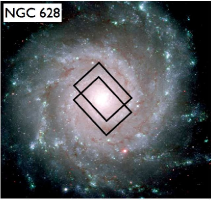
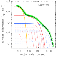
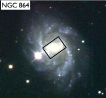
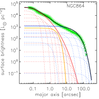
Figure 1: Multi-colour SDSS images, with the SAURON fields-of-view overlaid (black rectangles), and multi-Gaussian expansion models of the galaxies NGC 628 (left two panels) and NGC 864 (right two panels). Green asterisks represent the observed luminosity profiles. The black thick curves show the sum of the individual Gaussians (dotted curves) of the three components: nucleus (yellow), Sérsic bulge (red) and exponential disc (blue).

To infer the mass distributions of the 18 SAURON galaxies, we use the photometric bulge-disc decompositions of the total H-band surface brightness profile, as presented in Ganda (2007) and G09 (see also Sec. 2.3). These models represent each galaxy’s profile as the superposition of an exponential disc and a Sérsic bulge.

The galaxies in our sample can contain a significant amount of interstellar dust, which is mostly transparent at near-infrared wavelengths. The extinction $A_{H}$ is roughly a factor of 8 lower than the extinction $A_{V}$ (Rieke & Lebofsky, 1985), so we do not apply an internal extinction correction. Additionally, the near-infrared is considered as a good tracer of the stellar mass in galaxies as the light is dominated by old stars (Frogel, 1988; Rix & Zaritsky, 1995; Lilly, 1989), although there is some concern that this might be not true due to uncertain influence of intermediate age populations (Maraston 2005; Conroy, Gunn & White 2009; Melbourne et al. 2012; Zibetti, Charlot & Rix 2009; Zibetti et al. 2013).

Ganda (2007) and G09 use a one-dimensional MGE decomposition (Emsellem, Monnet & Bacon, 1994) of the bulge and disk profiles, using the implementation of Cappellari (2002). They adopt 10 Gaussians to represent the discs and between 13 and 19 Gaussians to represent the bulges. The fits to the one-dimensional profiles are excellent for all galaxies, but the MGE is not applied to the two-dimensional images.

Most of the galaxies (16 out of 18) display a clear light excess above the Sérsic fit to the bulge, which can be attributed to a bright nuclear star cluster (Böker et al., 2002), where a luminous mass contributes to the kinematics in the inner regions. For these galaxies, we amend the MGE decomposition of (Ganda, 2007, Chapter 5; Sec.5.4.) by including one additional, circular Gaussian to accurately represent the light excess in the centre.

Figure 1 shows the MGE light models of two representative galaxies in our sample. The green asterisks indicate their observed light profiles. The black thick curves represent the sum of the individual gaussians (dotted lines) of the three components: nucleus (yellow), Sérsic bulge (red), and exponential disc (blue), which are marked in Appendix A with index of 0, 1 and 2, respectively. NGC 628 (left panels) is an example of a very good fit to the data, which is typical for the majority of our galaxies. However, there are a few exceptions with mismatches due to bars or prominent spiral arms. These are NGC 864 (Figure 1, right panel), NGC 772, and NGC 1042. Nevertheless, we considered the MGE fits to these three galaxies to be satisfactory for our needs, because fitting non-symmetric features could lead to uneven representation of the galaxies’ surface brightness profiles, and hence, gravitational potentials. We converted the resulting peak surface brightnesses of the Gaussians into physical units of $L_{\odot}\leavevmode\nobreak\ \mbox{pc}^{-2}$, taking the absolute magnitude of the Sun $M_{H,\sun}=3.32$ (Binney & Merrifield, 1998).

4.2 Stellar kinematic maps

We measured the stellar kinematics using the penalised pixel-fitting (pPXF) method of Cappellari & Emsellem (2004). For spectral templates, we used a sub-sample of the MILES stellar library (Sánchez-Blázquez et al., 2006; Falcón-Barroso et al., 2011), containing $\sim$ 115 stars that span a large range in atmospheric parameters such as surface gravity, effective temperature and metallicity. We convolve the MILES models of stars from their original spectral resolution to that of the data. This is done by convolving with a Gaussian with dispersion equal to the difference in quadrature between the final and starting resolution. The pPXF method fits a non-negative linear combination of these stellar template spectra, convolved with the Gaussian velocity distribution, to each galaxy spectrum by chi-square minimisation. The higher-order Gauss-Hermite moments h3 and h4 are not included in this fit as free parameters. The spectral regions affected by emission lines were masked out during this process. A low-order polynomial (typically sixth degree) is included in the fit to account for small differences in the flux calibration between the galaxy and the template spectra. This analysis yields the stellar mean velocity ($V$) and stellar velocity dispersion ($\sigma$) for each bin. Their errors are estimated through Monte-Carlo simulations with noise added to the galaxy’s best fitting model spectrum.

The SAURON instrumental resolution is 105 km s^-1while the measured velocity dispersions of our galaxies can be significantly below that level. Emsellem et al. (2004) used Monte-Carlo simulations to show that the intrinsic velocity dispersion is still well recovered. For a spectrum with signal-to-noise of $\approx{60}$ and $\sigma\approx{50}$ km s^-1, the pPXF method will give velocity dispersions differing from the intrinsic ones by $\sim 10$ km s^-1, consistent with the measured errors. We might even expect larger uncertainties for some of our galaxies (e.g., NGC 3346, NGC 4487 and NGC 5585), which own central velocity dispersions below this limit. On the other hand, recent papers put forward evidence that our adopted approach could accurately recover the intrinsic velocity dispersion to better than 10% precision given the simulations of Toloba et al. 2011 and Ryś, Falcón-Barroso & van de Ven 2013 and our high S/N ($\sim 60$) in each Voronoi bin.

In Fig. 2 we show the stellar kinematic maps of our sample of 18 late-type spiral galaxies resulting from the pPXF fits. The first column shows the stellar flux in arbitrary units on a logarithmic scale. The next two columns display $V$ and $\sigma$ maps in km s^-1 respectively. We over-plotted the surface brightness contours of the galaxies as derived from their intensity maps.

For some of our galaxies, the centre position was not accurately determined during the data reduction due to foreground stars and dust lanes, which in some cases caused a significant offset in the measurement of the systemic velocity V_sys. Therefore, we use the velocity field symmetrisation method described in Appendix A of van den Bosch & de Zeeuw (2010) to estimate a robust V_sys. This method assumes that the velocity field (1) is symmetric with respect to the galaxy centre, (2) is uncorrelated and (3) varies linearly along the spatial coordinates. Then, for each position that has a counterpart, it computes their weighted mean velocities and combined errors (rejecting data with errors $>2.0$ km s^-1). In this way we obtain a robust estimate of V_sys for each galaxy (see Table 1).

Galaxies with more concentrated light distributions generally have larger central peaks in their velocity dispersion fields. Elliptical galaxies usually have radially decreasing $\sigma$ (D’Onofrio et al., 1995), and this is also the case for many early-type spirals, as a result of a centrally concentrated bulge. But for very late-type spirals, we expect the $\sigma$ field to be either flat (due to their lower bulge-to-disc ratios) or with a central decrease, because of cold components or counter-rotating discs (Falcón-Barroso et al. 2006). In comparison with early-type galaxies, the bulges of the late-type spirals are smaller and have lower surface brightness (Yoachim & Dalcanton, 2006, G09). Martinsson et al. (2013b) also find that $\sigma$ generally decreases with radius with an $e$-folding length that is twice the photometric disc scale length. Thus, the variety seen in $\sigma$ profiles of SAURON galaxies might be also due to their limited radial coverage, ranging between 0.4 and 1.2 scale lengths.

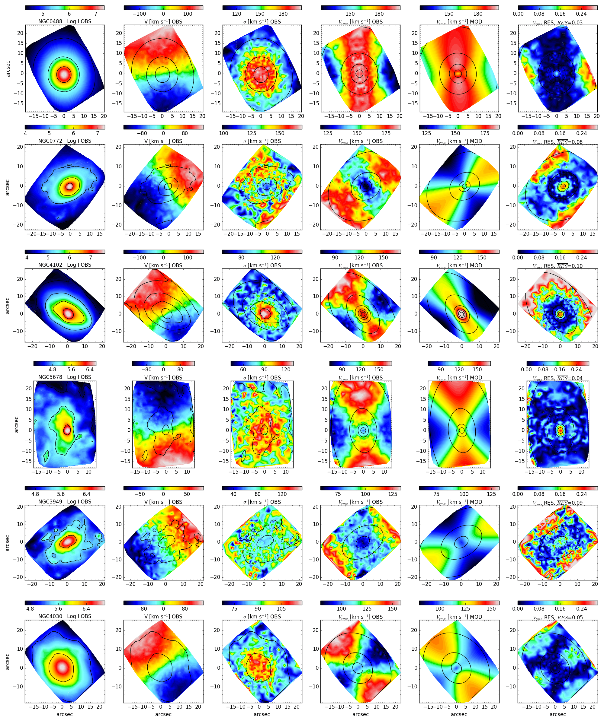
Figure 2: Stellar kinematics and second moment maps of our sample of 18 galaxies. First column: stellar flux derived from the collapsed data cubes; second and third column: observed mean line-of-sight velocity and velocity dispersion; fourth-sixth columns with overplotted MGEs contours: second moment maps $V_{\mathrm{rms}}=\sqrt{V^{2}+\sigma^{2}}$ of the data and the model, and the residual maps RES=$|(V_{\mathrm{rms,obs}}/V_{\mathrm{rms,mod}})-1|$ with median values $\overline{\emph{RES}}$.

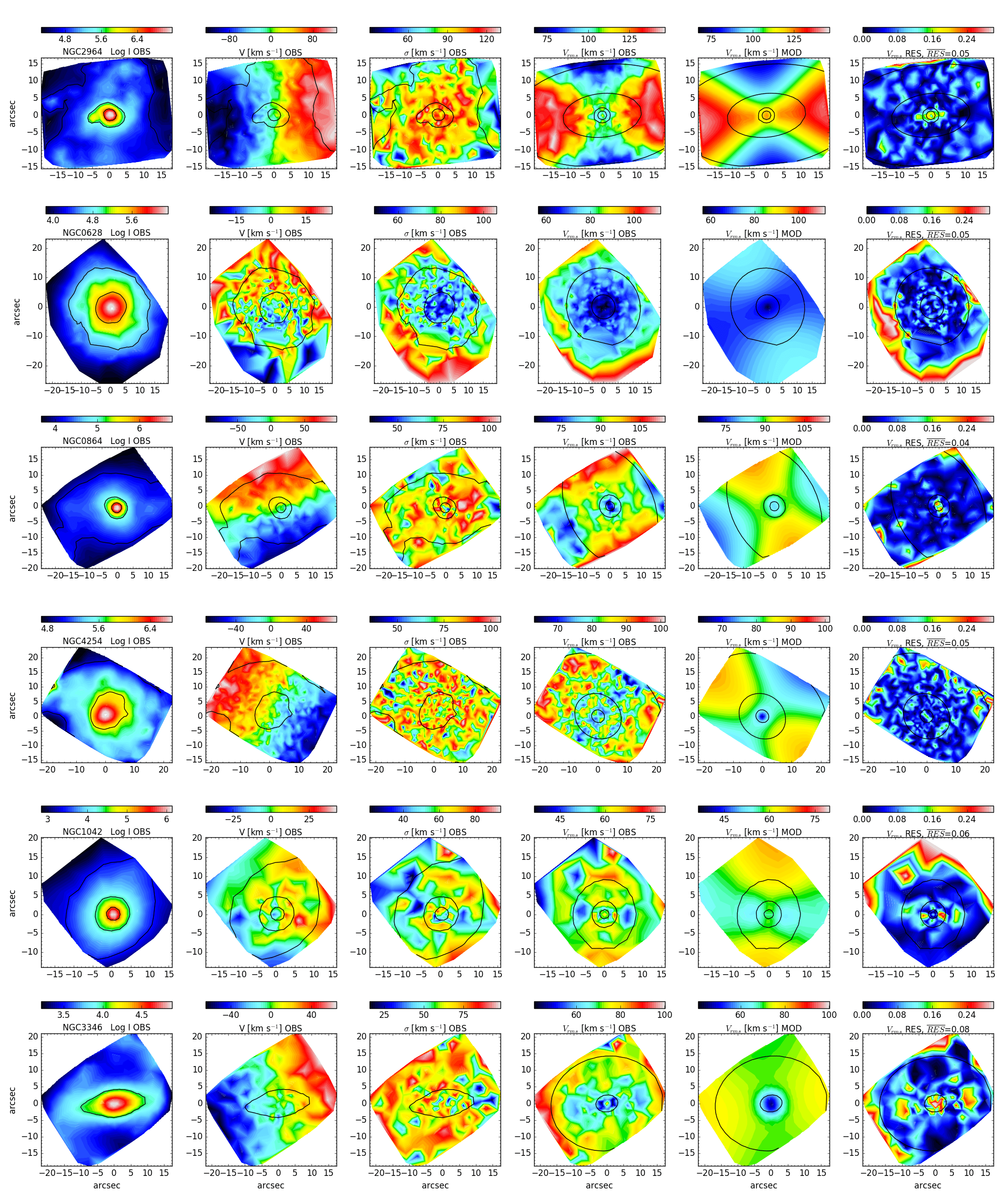
Figure 2: – continuation

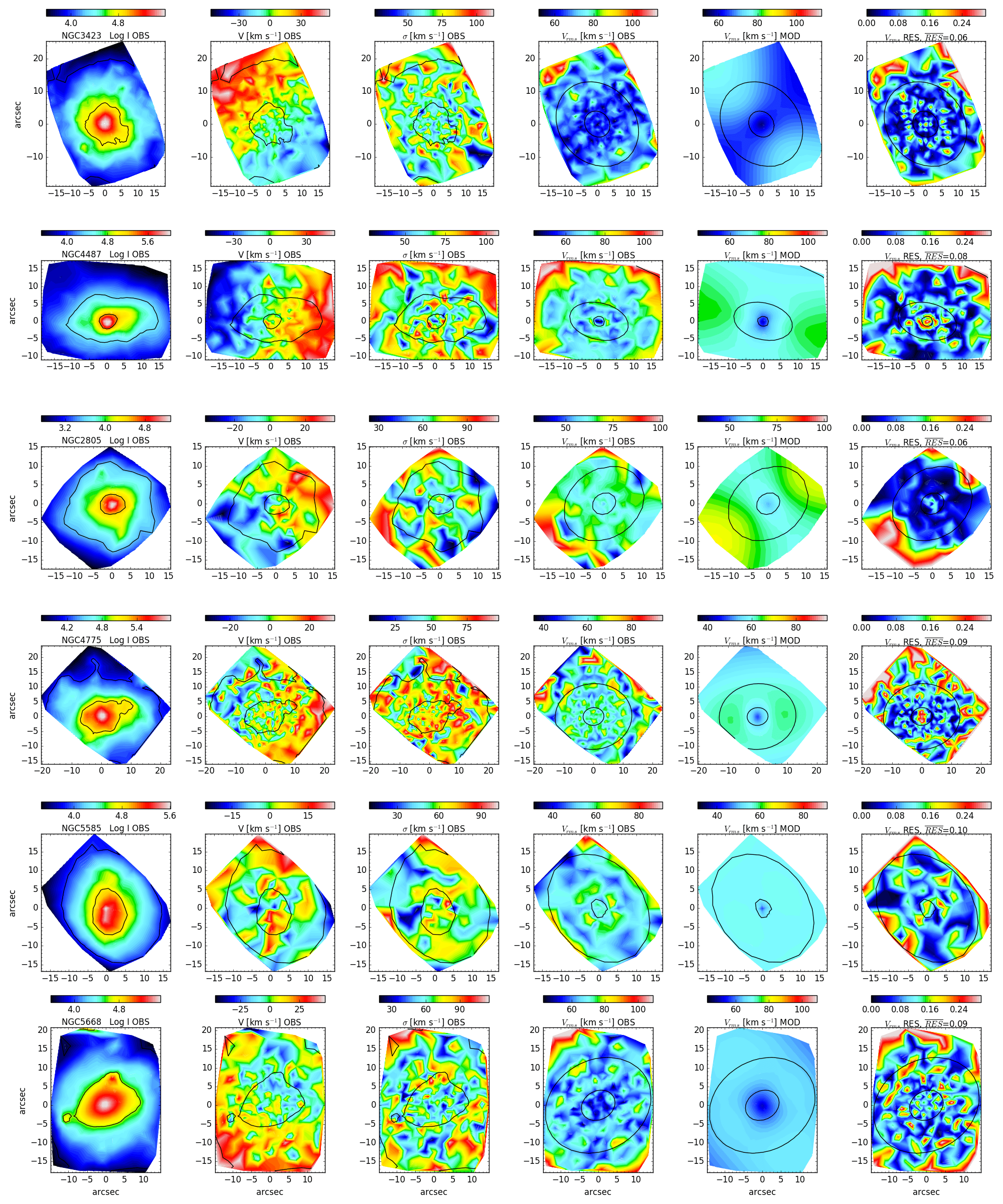
Figure 2: – continuation

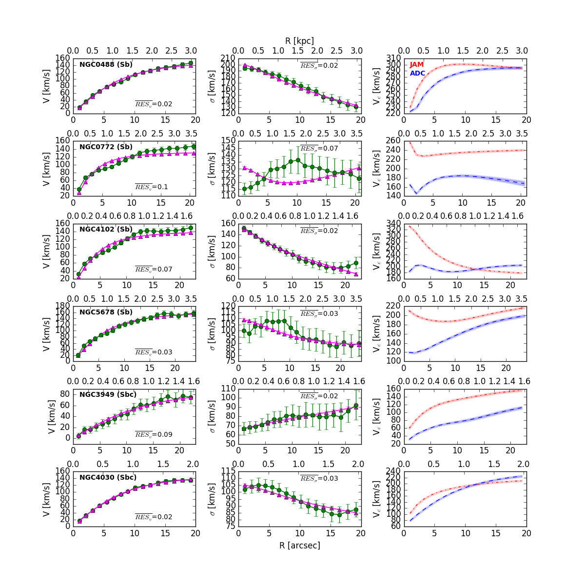
Figure 3: Rotation curves of our sample of 18 galaxies using ADC-MCMC and JAM-MCMC methods. First column: stellar mean line-of-sight velocity $V$ (green filled circles) and its MCMC fit of simple analytic functions (magenta filled triangles); second column: stellar line-of-sight velocity dispersion $\sigma$ (green filled circles) and its MCMC fit of simple analytic functions (magenta filled triangles); third column: circular velocity curves derived from ADC-MCMC (blue dashed line) and JAM-MCMC (red dashed-dot line) methods. The bands indicate the uncertainties of the presented circular curves. There is a significant and systematic offset between the two models, where ADC gives lower values of the circular velocity curves than JAM.

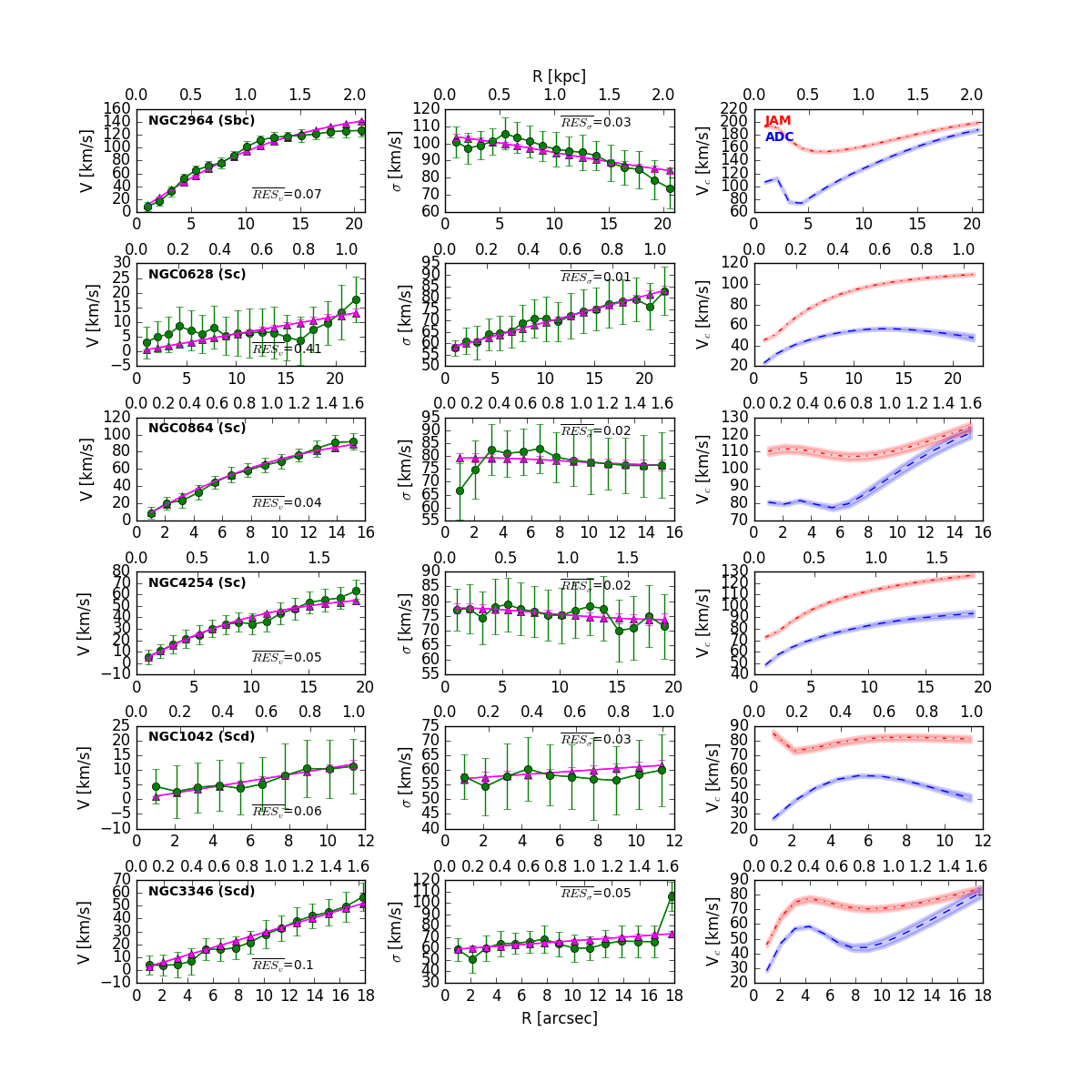
Figure 3: – continuation

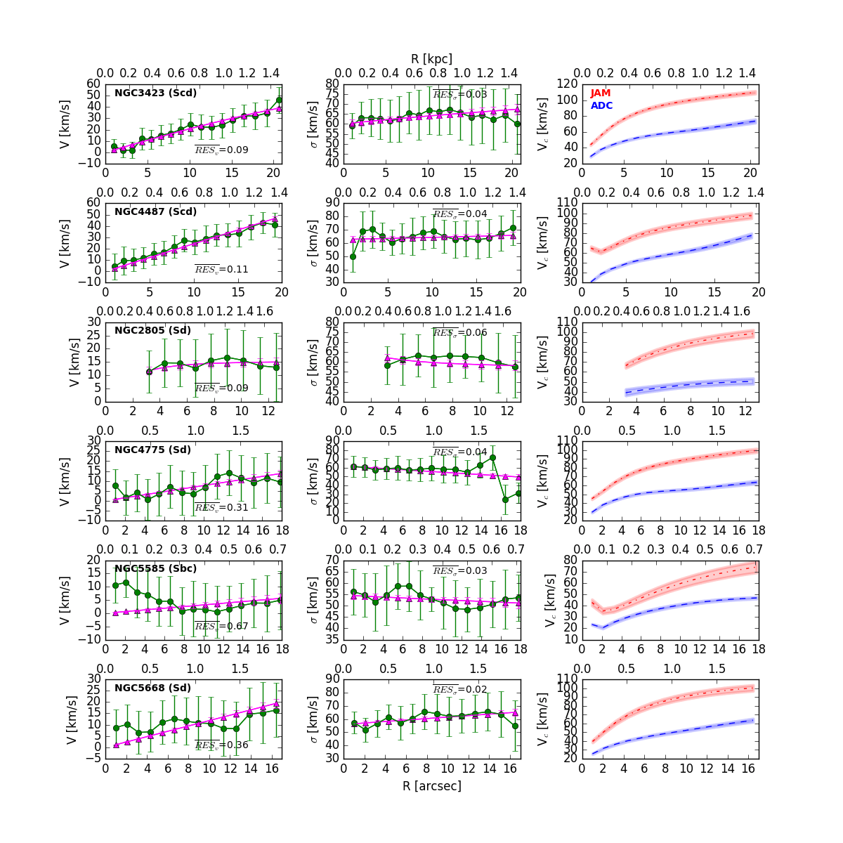
Figure 3: – continuation

4.3 Markov Chain Monte Carlo

To obtain reliable circular velocity curves and associated uncertainties, we assume these properties are random variables viewed in a Bayesian framework. We then applied Markov chain Monte Carlo (MCMC) to estimate these variables under both the ADC and JAM model approaches. We used the EMCEE code of Foreman-Mackey et al. (2013), an implementation of an affine invariant ensemble sampler for the MCMC method of parameter estimation, together with JAM code (Cappellari 2008) and our own ADC routines all of which are implemented in PYTHON. This approach allows a robust understanding of the uncertainties in the modelling combined with their dependance on assumptions, which is particularly important since we ultimately compare ADC and JAM results.

4.3.1 ADC-MCMC modeling

Table 2: Summaries of the posterior distribution for the ADC model. The value is the median of the distribution and the uncertainties are the 25th and 75th percentiles of the data corresponding to the median absolute deviation. Columns list: (1) Galaxy identifier; (2) Hubble type (NED); (3) and (4) $\overline{v_{\phi}}$ power-law fit with $v_{\infty}$ in km s^-1 and $R_{c}$ in arcsec (see Eq. 15); (5) $\overline{v_{\phi}}$ linear fit with slope $k_{v}$ (see Eq. 16); (6) and (7) $\sigma_{R}$ linear fit to the deprojected line-of-sight velocity dispersion with y-intercept $\sigma_{0}$ in km s^-1 and slope $k_{\sigma}$ (see Eq. 17); (8) azimuthal velocity anisotropy; (9) Goodness of ADC-MCMC fits (Sec. 4.3.1

)

Best fit parameters
		ADC-MCMC method
NGC	Type	$v_{\infty}$	$R_{c}$	$k_{v}$	$\sigma_{0}$	$k_{\sigma}$	$\beta_{z}^{\mathrm{ADC}}$	Good Fit
(1)	(2)	(3)	(4)	(5)	(6)	(7)	(8)	(9)
NGC0488	SA(r)b	$234.648^{+2.532}_{-2.546}$	$9.572^{+0.189}_{-0.194}$	$--$	$240.755^{+0.652}_{-0.657}$	$-2.972^{+0.149}_{-0.150}$	$0.529^{+0.015}_{-0.014}$	Yes
NGC0772	SA(s)b	$170.975^{+1.610}_{-1.670}$	$4.484^{+0.119}_{-0.117}$	$--$	$153.893^{+0.672}_{-0.646}$	$2.256^{+0.208}_{-0.200}$	$0.724^{+0.030}_{-0.031}$	Yes
NGC4102	SAB(s)b	$165.69^{+1.750}_{-1.626}$	$6.008^{+0.145}_{-0.139}$	$--$	$145.888^{+0.674}_{-0.667}$	$-3.031^{+0.116}_{-0.118}$	$-0.398^{+0.067}_{-0.069}$	Yes
NGC5678	SAB(rs)b	$187.225^{+2.392}_{-2.344}$	$8.57^{+0.260}_{-0.247}$	$--$	$111.533^{+0.656}_{-0.649}$	$0.059^{+0.166}_{-0.161}$	$0.185^{+0.121}_{-0.125}$	Yes
NGC3949	SA(s)bc	$115.368^{+3.287}_{-3.250}$	$15.897^{+0.572}_{-0.585}$	$--$	$61.838^{+0.667}_{-0.667}$	$1.51^{+0.208}_{-0.197}$	$-0.296^{+0.158}_{-0.166}$	Yes
NGC4030	SA(s)bc	$226.882^{+2.808}_{-2.731}$	$10.02^{+0.230}_{-0.230}$	$--$	$108.476^{+0.651}_{-0.653}$	$-0.609^{+0.112}_{-0.104}$	$0.089^{+0.039}_{-0.041}$	Yes
NGC2964	SAB(r)bc	$210.274^{+4.006}_{-3.998}$	$16.415^{+0.496}_{-0.506}$	$--$	$93.049^{+0.666}_{-0.677}$	$-0.497^{+0.161}_{-0.148}$	$-0.996^{+0.195}_{-0.185}$	Yes
NGC0628	SA(s)c	$--$	$--$	$0.961^{+0.107}_{-0.105}$	$59.047^{+0.680}_{-0.708}$	$1.197^{+0.142}_{-0.138}$	$0.086^{+0.072}_{-0.078}$	No
NGC0864	SAB(rs)c	$152.711^{+4.104}_{-4.050}$	$12.886^{+0.511}_{-0.506}$	$--$	$78.378^{+0.682}_{-0.682}$	$0.322^{+0.273}_{-0.262}$	$-0.032^{+0.136}_{-0.146}$	Yes
NGC4254	SA(s)c	$92.836^{+3.071}_{-3.164}$	$12.984^{+0.603}_{-0.600}$	$--$	$76.031^{+0.691}_{-0.664}$	$0.17^{+0.194}_{-0.194}$	$-0.078^{+0.105}_{-0.109}$	Yes
NGC1042	SAB(rs)cd	$--$	$--$	$1.432^{+0.169}_{-0.175}$	$53.823^{+0.714}_{-0.681}$	$0.422^{+0.223}_{-0.224}$	$-0.225^{+0.170}_{-0.186}$	Yes
NGC3346	SB(rs)cd	$--$	$--$	$4.387^{+0.160}_{-0.160}$	$57.403^{+0.701}_{-0.687}$	$0.782^{+0.217}_{-0.220}$	$-0.082^{+0.134}_{-0.150}$	Yes
NGC3423	SA(s)cd	$125.645^{+4.941}_{-4.882}$	$39.504^{+0.641}_{-0.615}$	$--$	$56.791^{+0.710}_{-0.700}$	$0.409^{+0.191}_{-0.184}$	$-0.215^{+0.135}_{-0.141}$	Yes
NGC4487	SAB(rs)cd	$--$	$--$	$3.025^{+0.125}_{-0.126}$	$60.728^{+0.649}_{-0.638}$	$0.156^{+0.212}_{-0.200}$	$-0.183^{+0.229}_{-0.245}$	Yes
NGC2805	SAB(rs)d	$22.525^{+2.492}_{-2.490}$	$2.635^{+0.629}_{-0.627}$	$--$	$67.312^{+0.657}_{-0.662}$	$-0.097^{+0.288}_{-0.295}$	$-0.001^{+0.122}_{-0.136}$	Yes
NGC4775	SA(s)d	$--$	$--$	$1.380^{+0.198}_{-0.201}$	$58.592^{+0.696}_{-0.704}$	$-0.654^{+0.208}_{-0.205}$	$-0.176^{+0.141}_{-0.150}$	No
NGC5585	SAB(s)d	$--$	$--$	$0.396^{+0.131}_{-0.126}$	$49.839^{+0.639}_{-0.638}$	$-0.173^{+0.174}_{-0.152}$	$-0.558^{+0.231}_{-0.204}$	No
NGC5668	SA(s)d	$--$	$--$	$1.966^{+0.201}_{-0.203}$	$53.332^{+0.696}_{-0.666}$	$0.538^{+0.236}_{-0.235}$	$-0.153^{+0.129}_{-0.135}$	No

To infer circular velocity curves for our sample of galaxies using the ADC method (Sect. 3.3), we first need their kinematic profiles along the projected major axis. To this end, we use the kinemetry package of Krajnović et al. (2006) that is based on harmonic expansion of two-dimensional maps along ellipses. We extract the observed mean velocity $V_{\mathrm{maj}}$ and velocity dispersion $\sigma_{\mathrm{maj}}$ profiles along ellipses with fixed axis ratio of the galaxies ($q=1-\epsilon$) and photometric position angle, where $\epsilon$ and $PA$ are shown in Table 1. However, for galaxies NGC3346, NGC4775 and NGC5668, we calculate the axis ratio $q$ from the adopted inclination $\emph{i}=\emph{i}^{MGE}$ using eq. 1 (see Sec. 2.1) .

Then under the ’thin-disc’ assumption we obtain the intrinsic mean velocity $\overline{v_{\phi}}$ and radial velocity dispersion $\sigma_{R}$ profiles from the observed profiles as:

$$V_{\mathrm{maj}} = V_{\mathrm{sys}}+\overline{v_{\phi}}\sin i,$$ (11)

$$\sigma_{\mathrm{maj}}^{2} = \sigma_{\phi}^{2}\sin^{2}i+\sigma_{z}^{2}\cos^{2}i$$ (12)

$$= \sigma_{R}^{2}\left[\frac{(1+\alpha_{R})}{2}\sin^{2}i+(1-\beta_{z})\cos^{2}i\right],$$

with systematic velocity $V_{\mathrm{sys}}$ and adopted inclination $i$ from Table 1. To get to equation (12), we have used $\sigma_{\phi}^{2}/\sigma_{R}^{2}=(1+\alpha_{R})/2$ under the assumptions that the velocity ellipsoid is aligned with the cylindrical coordinate system and symmetric around $v_{\phi}=\overline{v_{\phi}}$ (see Section 3.3). As before, $\beta_{z}=1-\sigma_{z}^{2}/\sigma_{R}^{2}$ is the velocity anisotropy in the meridional plane, and $\alpha_{R}=\partial\ln\overline{v_{\phi}}/\partial\ln R$ is the radial logarithmic gradient of the intrinsic mean velocity.

Given the assumptions of the ADC approach, we relate the model parameters to the observed data as follows:

$$V=\overline{v_{\phi}}\sin i,$$ (13)

$$\sigma=\sigma_{R}\sqrt{0.5(1+\alpha_{R})\sin^{2}i+(1-\beta_{z}^{\mathrm{ADC}})\cos^{2}i},$$ (14)

where $V=V_{\mathrm{maj}}-V_{\mathrm{sys}}$ and $\sigma=\sigma_{\mathrm{maj}}$. To avoid numerical noise in the derivatives, we express $\overline{v_{\phi}}$ and $\sigma_{R}$ using a smooth, analytic functional forms and then compute the derivatives explicitly.

As an analytical representation for $v_{\phi}$, we use the ’power-law’ prescription of Evans & de Zeeuw (1994, eq.2.11), which in the equatorial plane ($z=0$) and assuming flat rotation curve, becomes

$$\overline{v_{\phi}}(R)=\frac{v_{\infty}R}{\sqrt{R_{c}^{2}+R^{2}}},$$ (15)

where $v_{\infty}$ is the asymptotic velocity and $R_{c}$ is the core radius. This model describes a rotation curve that increases linearly with radius $\propto(v_{\infty}/R_{c})\,R$ when $R\ll R_{c}$, and flattens to the value $v_{\infty}$ when $R\gg R_{c}$. However, in several cases the velocity profile shows little indication of flattening the observed region. In such cases, the core radius $R_{c}$ is not well constrained and fitting Eq. (15) would lead to unphysical values for both $R_{c}$ and $v_{\infty}$. Such galaxies are in the regime of $R\ll R_{c}$ and we adopt a linear solid-body rotation instead:

$$\overline{v_{\phi}}(R)=k_{v}\,R,$$ (16)

where $k_{v}$ is the linear coefficient.
For $\sigma_{R}$, we use a linear expression of the form

$$\sigma_{R}(R)=\sigma_{0}+k_{\sigma}\,R$$ (17)

where $\sigma_{0}$ and $k_{\sigma}$ are free parameters. We find the linear fits to the $\sigma_{R}$ profiles are broadly representative, although the model does not reproduce the central part of the $\sigma_{R}$ profiles for some of the galaxies (e.g., NGC 772, NGC 5678 and NGC 864) due to the marked dips in $\sigma$ in the central parts of the galaxies (Falcón-Barroso et al. 2006). Such a descrease in the observed stellar velocity dispersion might be the result of a small dynamically cold component or counter-rotating disc of high surface brightness that obscures the bulge, dominating the luminosity-derived kinematic measurements (Falcón-Barroso et al. 2006) or due to $e$-folding length of our galaxies (see Martinsson et al. 2013b).

To apply a Bayesian framework to the problem, we consider the free parameters of the model to be random variables and then calculate their posterior distributions using MCMC. We model 5 free parameters for the galaxies in the power-law model for $v_{\phi}$ ($v_{\infty}$, $R_{c}$, $\sigma_{0}$, $k_{\sigma}$, $\beta_{z}^{\mathrm{ADC}}$) and 4 free parameters ($k_{v}$, $\sigma_{0}$, $k_{\sigma}$, $\beta_{z}^{\mathrm{ADC}}$) for the galaxies with linear models for $v_{\phi}$. For these vectors of parameters $\boldsymbol{\theta}$, we compute model profiles for $V_{\mathrm{MOD}}$ and $\sigma_{\mathrm{MOD}}$ using Eq.(13) and (14). These profiles are compared to observed data using a chi-squared statistic, summing over radius positions with normalization set by the uncertainties in the observed data ($\delta V_{\mathrm{OBS}}$ and $\delta\sigma_{\mathrm{OBS}}$):

$$\chi^{2} = \sum_{k}[V_{\mathrm{MOD},k}(\boldsymbol{\theta})-V_{\mathrm{OBS},k}]^{2}/(\delta V_{\mathrm{OBS},k}^{2})$$ (18)

$$+ \sum_{k}[\sigma_{\mathrm{MOD},k}(\boldsymbol{\theta})-\sigma_{\mathrm{OBS},k}]^{2}/(\delta\sigma_{\mathrm{OBS},k}^{2}).$$

We adopt a log-probability function for the parameters given the data as $\mathcal{L}(\boldsymbol{\theta}|V_{\mathrm{OBS}},\sigma_{\mathrm{OBS}})=-\chi^{2}+\mathbf{p}$, where $\mathbf{p}$ is a set of priors. We adopt uniform prior distributions for our parameters on fixed ranges: $v_{\infty}\in[0,400]$ km s^-1, $R_{c}\in[0^{\prime},50^{\prime\prime}]$ , $k_{v}\in[0,10]$ km s^-1 arcsec^-1, $\sigma_{0}\in[0,300]$ km s^-1, $k_{\sigma}\in[-5,5]$ km s^-1 arcsec^-1 and $\beta_{z}^{\mathrm{ADC}}\in[-1,+1]$. Only for one galaxy (NGC2964) we had to expand the range of the walkers to $\beta_{z}^{\mathrm{ADC}}\in[-1.5,+1]$, since the distribution peaked at $\beta_{z}^{\mathrm{ADC}}=-0.996$.

We run the ADC-MCMC code with 60 walkers (i.e., members of the ensemble sampler), which have initial position set by the prior information and physical information. We use a small random distribution around the parameters: $v_{\infty}$, $R_{c}$, $k_{v}$, $\sigma_{0}$, $k_{\sigma}$, which are adopted from the least-squares minimisation routine mpfit in IDL to find the values that minimize Eq. 18. We then start the walkers around the optimized values in a normal distribution with scale determined by the uncertainties in the fit. The walkers of the parameter $\beta_{z}^{\mathrm{ADC}}$ were allowed to move freely in the parameter space. On the other hand, the inclination of the galaxies is fixed to the value presented in column 6 of Table 1. The MCMC code samples the posterior distribution, using 400 steps for burn-in and 1000 steps for sampling. We find that all walkers converge after $\sim 50$ steps of burn-in to sample a similar distribution indicating a well-sampled unimodal posterior distribution. We summarize the posterior distributions for the parameters in Table 2 of this paper. Additionally, we assign a quality flag to each ADC-MCMC model in Table 2 depending on the residual of the V profile ($RES_{v}=|(V_{\mathrm{obs}}/V_{\mathrm{mod}})-1|$) and $\sigma$ profile ($RES_{\sigma}=|(\sigma_{\mathrm{obs}}/\sigma_{\mathrm{mod}})-1|$), where the label "Yes/No" correspond to "Good/Bad" fit, respectively. Bad fit label is associated to galaxies (i.e., NGC0628, NGC4775, NGC5585 and NGC5668) if the median value of one of their residuals ($\overline{RES_{v}}$ or $\overline{RES_{\sigma}}$) is larger than 0.3. The burn-in chains, posterior chains and corner plots of ADC-MCMC method are shown in Appendix C.

We present the results of the analysis in Fig. 3. In the first column, we show the observed mean line-of-sight velocity $V$ (filled green circles) and its fiting function (Eq. 13, filled magenta triangles). The galaxies are ordered by their morphological type from Sb to Sd. We observe that Sb–Sc galaxies (at $R_{e}/5$) have higher observed velocity in contrast to Scd–Sd. We adopt a power-law model function to most of the $v_{\phi}$ radial profiles, except for the galaxies – NGC 0628, NGC 1042, NGC 3346, NGC 4487, NGC 4775, NGC 5585 and NGC 5668, which require a linear function.

In the second column of Fig. 3, we present the observed line-of-sight velocity dispersion $\sigma$ profiles (filled green circles) and its fiting function (Eq. 14, filled magenta triangles). The $\sigma$ profiles are more varied than the $V$ profiles. Some velocity dispersion profiles show an almost-linear decrease or increase with radius on the whole radial range available, some are flat, and others have a more complex behaviour that seems difficult to reproduce with a linear function. Sb–Sbc galaxies (at $R_{e}/5$) are characterised by high observed velocity dispersion $\sigma$ with respect to Sc–Sd. Most of our Sb-Sc galaxies have regular velocity fields with well-defined axisymmetric rotation and high amplitude, while Sd velocity fields show more complex structure and lower amplitude of rotation. In our sample we have four types of $\sigma$ behaviour: decreasing outward (NGC 4102), increasing outward (NGC 3949), a central $\sigma$-dip (NGC 0772) or flat (NGC 4775).

We estimate the uncertainty of the velocity and velocity dispersion profiles at each radius (see Fig. 3) from the corresponding error maps since the provided uncertainties from kinemetry routine are unrealistically small ($\sim$ 1 km^-1). Thus, we took the absolute value of the median of the velocity bins and the median of the velocity dispersion bins within each annulus defined by kinemetry routine.

4.3.2 JAM-MCMC modeling

As described in Sect. 3, we use a solution of the axisymmetric Jeans equations based on a Multi-Gaussian Expansion (MGE) of the intrinsic luminosity density to predict the observed second velocity moment $V_{\mathrm{rms}}=\sqrt{V^{2}+\sigma^{2}}$ (Cappellari 2008). The solution has a constant meridional plane velocity anisotropy $\beta_{z}^{\mathrm{JAM}}$ and constant mass-to-light ratio $\Upsilon_{\mathrm{tot}}$ within the galaxy. Our analysis does not account for the variation of $V_{\mathrm{rms}}$ within each Voronoi bin. Such variations will cause the averaged $V_{\mathrm{rms}}$ in a bin to be larger than the intrinsic $V_{\mathrm{rms}}$ along a ray, as evaluated by the JAM code. We do not anticipate this effect to bias our results significantly: since the surface brightness decreases with $R$, the larger Voronoi bins are found in the outer regions of the galaxies where the variation in the $V_{\mathrm{rms}}$ surface is low. At small $R$, where the variation with position can be significant, the higher surface brightness means the bins are smaller.

We symmetrize our observed $V_{\mathrm{rms}}$ fields in order to avoid outliers in the data (see Cappellari et al. 2015). In this way, the results will be not influenced by a few deviant values. This is especially important in the case of the MCMC method application, where the best fit $V_{\mathrm{rms}}$ model rely on $\chi^{2}$-statistics. Moreover, the symmetrization renders the $V_{\mathrm{rms}}$ field axisymmetric which is the approximation consider by JAM. At the same time we symmetrize the variance of the $V_{\mathrm{rms}}$ field:

$$\Delta V_{\mathrm{rms}}=2\sqrt{\mathrm{sym}\left\{\frac{(\Delta V\cdot V)^{2}+(\Delta\sigma\cdot\sigma)^{2})}{V_{\mathrm{rms}}^{2}}\right\}},\\$$ (19)

where the term $\mathrm{sym}\left\{...\right\}$ indicates the symmetrized variance of $V_{\mathrm{rms}}$ field.

For this purpose we use the code presented in Cappellari et al. (2015). The procedure interpolates the bin values over a new grid generated by permuting the $j$th-bin coordinates as follow:

$$x_{j}\rightarrow(x_{j},-x_{j},x_{j},-x_{j}),$$

$$y_{j}\rightarrow(y_{j},y_{j},-y_{j},-y_{j}).$$ (20)

This operation generates three additional velocity fields (the first permutation obtained by $x_{j},y_{j}$ corresponds to the original velocity field). Finally, the symmetrized velocity field is the mean of the four coordinate-permuted velocity fields. Given this, equation (19) reduces to the common addition of the error in quadrature:

$$\Delta V_{\mathrm{rms}}=2\sqrt{\frac{Q}{4}},$$ (21)

where $Q=\Delta V_{\mathrm{rms}}^{2}(x_{j},y_{j})+\Delta V_{\mathrm{rms}}^{2}(-x_{j},y_{j})+\Delta V_{\mathrm{rms}}^{2}(x_{j},-y_{j})+\Delta V_{\mathrm{rms}}^{2}(-x_{j},-y_{j})$, and
$\Delta V_{\mathrm{rms}}^{2}=(\Delta V\cdot V)^{2}+(\Delta\sigma\cdot\sigma)^{2}$ of a certain permutation.

Although the interpolation is precise, the code does not consider the systematic effect that a given bin at $(x,y)$ position not always have a corresponding bin atat the other positions, e.g., (-x,y). To account for this, the final $V_{\mathrm{rms}}$ field error is set by the maximum of either the values from equation (19) or half the deviation between neighbors $V_{\mathrm{rms}}$ field bin values (M. Cappellari private communication, see also Morganti et al. 2013).

We formulate a parallel MCMC approach for determining the posterior parameter distributions of the JAM model. In this case, there are only 2 free parameters for all galaxies ($\beta_{z}^{\mathrm{JAM}}$ and $\Upsilon$). Because of the large computational expense of evaluating a JAM model, we run the JAM-MCMC code with only 30 walkers, though the model still converges using 100 steps for a burn-in and 200 steps for sampling. The prior distributions are taken to be uniform with, e.g., $\beta_{z}^{\mathrm{JAM}}\in[-1,+1]$ and $\Upsilon\in[0,10]\leavevmode\nobreak\ M_{\odot}/L_{\odot}$.

In JAM-MCMC method, we fix the inclination to the values in the column 6 of Table 1. For galaxies NGC3346, NGC4775, and NGC5668, we adopt $\emph{i}=\emph{i}^{\mathrm{MGE}}$ regarding to the minimum possible inclination condition of JAM model (see Sec. 3.2; eq. 8).

We use a similar log-likelihood statistic as we did for the ADC, except in this case, only the model and observed $V_{\mathrm{rms}}$ are compared. Summaries of the posterior distribution of parameters for JAM-MCMC model are presented in Table 3. The burn-in chains, posterior chains and corner plots are shown in Appendix B.

In the fourth to fifth columns of Fig. 2, we show the observed and the best fitting $V_{\mathrm{rms}}$ maps with over-plotted MGE contours. For all galaxies, the MGE contours are aligned with the surface brightness contours in position angle and ellipticity. In the sixth colum, we calculate the residual maps RES between the observations ($V_{\mathrm{rms,obs}}$) and the models ($V_{\mathrm{rms,mod}}$), where $RES$=$|(V_{\mathrm{rms,obs}}/V_{\mathrm{rms,mod}})-1|$. The median values of these residual maps $\overline{\emph{RES}}$ indicate that the uncertainties of JAM fit ranges between 3 % and 10 %. Note here that we do not count for systematics errors in these uncertainties. From the posterior distributions of JAM-MCMC method, we define the goodness of the fit with the label "Yes/No" for "Good/Bad" fit, respectively. Bad fit labels are associated to galaxies (i.e., NGC 4030, NGC 1042, NGC 3346), which do not have well defined posterior distributions of the velocity anisotropy $\beta^{\mathrm{JAM}}_{z}$ (see Appendix B and Table 3).

Further, we find that the JAM produces the best fits to the second velocity moment $V_{\mathrm{rms}}$ for Sb and Sc spirals (e.g., NGC 488, NGC 5678, and NGC 2964, characterised by fast-rotating discs) and the model gets worse for Scd and Sd galaxies. Given the observed values of $V$ and $\sigma$ show evidence for non-monotonic behaviour (Figure 2), the model provides an average representation of the data in the late-type galaxies. We stress that the values derived for the parameters are the posterior distributions given the data, subject to the assumptions of the model.

Table 3: Summaries of the posterior distribution for the JAM model. The value is the median of the distribution and the uncertainties are the 25th and 75th percentiles of the data corresponding to the median absolute deviation. Columns are: (1) Galaxy identifier; (2) Hubble type (NED); (3) Azimuthal velocity anisotropy; (4) Dynamical mass-to-light ratio in H-band; (5) Goodness of JAM-MCMC fit (Sec. 4.3.2)

Best fit parameters
		JAM-MCMC method
NGC	Type	$\Upsilon$	$\beta^{\mathrm{JAM}}_{z}$	Good Fit
(1)	(2)	(3)	(4)	(5)
0488	SA(r)b	$1.148^{+0.003}_{-0.003}$	$-0.223^{+0.018}_{-0.017}$	Yes
0772	SA(s)b	$1.024^{+0.005}_{-0.005}$	$-0.628^{+0.035}_{-0.036}$	Yes
4102	SAB(s)b	$0.618^{+0.002}_{-0.002}$	$0.157^{+0.009}_{-0.009}$	Yes
5678	SAB(rs)b	$1.237^{+0.008}_{-0.008}$	$-0.209^{+0.031}_{-0.031}$	Yes
3949	SA(s)bc	$1.380^{+0.020}_{-0.018}$	$0.137^{+0.030}_{-0.032}$	Yes
4030	SA(s)bc	$0.743^{+0.002}_{-0.002}$	$-0.997^{+0.003}_{-0.002}$	No
2964	SAB(r)bc	$1.371^{+0.017}_{-0.016}$	$0.164^{+0.025}_{-0.027}$	Yes
0628	SA(s)c	$1.153^{+0.016}_{-0.018}$	$-0.692^{+0.133}_{-0.134}$	Yes
0864	SAB(rs)c	$1.466^{+0.056}_{-0.058}$	$0.215^{+0.065}_{-0.073}$	Yes
4254	SA(s)c	$0.451^{+0.007}_{-0.008}$	$-0.105^{+0.057}_{-0.060}$	Yes
1042	SAB(rs)cd	$1.800^{+0.083}_{-0.103}$	$-0.480^{+0.274}_{-0.265}$	No
3346	SB(rs)cd	$2.201^{+0.106}_{-0.133}$	$-0.480^{+0.285}_{-0.288}$	No
3423	SA(s)cd	$2.008^{+0.064}_{-0.069}$	$-0.310^{+0.152}_{-0.187}$	Yes
4487	SAB(rs)cd	$2.068^{+0.118}_{-0.119}$	$0.466^{+0.056}_{-0.059}$	Yes
2805	SAB(rs)d	$1.945^{+0.145}_{-0.162}$	$-0.141^{+0.277}_{-0.332}$	Yes
4775	SA(s)d	$1.043^{+0.042}_{-0.040}$	$0.331^{+0.087}_{-0.119}$	Yes
5585	SAB(s)d	$3.538^{+0.482}_{-0.491}$	$0.317^{+0.163}_{-0.193}$	Yes
5668	SA(s)d	$1.222^{+0.081}_{-0.069}$	$0.684^{+0.036}_{-0.045}$	Yes

5 Comparing circular velocity curves

In order to compare the two modelling approaches ADC and JAM, we first combine the measured deprojected stellar velocity profile $\overline{v_{\phi}}$ and radial dispersion profile $\sigma_{R}$. Next, we derive the circular velocity curve $v_{c,\mathrm{ADC}}$ using the asymmetric drift correction (ADC) formula in equation (10). These data are indicated by the blue-filled-pentagon curves with uncertainties derived from the transformed posterior distributions of ADC-MCMC results. Second, we construct axisymmetric Jeans models (JAM) that fit the combined observed stellar mean velocity and velocity dispersion fields, we use Equation (6) to obtain the circular velocity curve for each galaxy. The resulting $v_{c,\mathrm{JAM}}$ curves from the best-fit JAM model are plotted as red-filled-squares curves in Fig. 3 with their uncertainty from JAM-MCMC code. For all galaxies, ADC approach gives lower measurements of the circular velocity curve in comparison with the values obtained from JAM models for at least part of the radial range. To quantify these differences, we plot in Fig. 4 the velocity ratio between $v_{\mathrm{c,JAM}}$ and $v_{\mathrm{c,ADC}}$.

Overall, the velocity discrepancy for Sb-Sbc galaxies is larger in the inner parts ($R<R_{e}/5$) and decreases in the outer parts ($>R_{e}/5$), while for Scd-Sd galaxies the velocity discrepancy is constant or even increases in the outer parts.

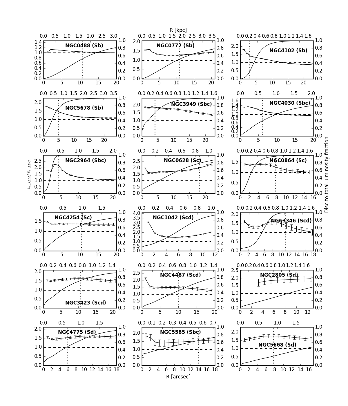
Figure 4: Velocity ratio between $v_{\mathrm{c,JAM}}$ best fit and $v_{\mathrm{c,ADC}}$, where the bar indicates the typical uncertainty. Over-plotted are the disc-to-total luminosity fraction (thin solid line), the $R_{e}/5$ (dotted line) where $R_{e}$ is the MGE effective radius, and the one-to-one relation of the velocity ratio (dashed line). The significant differences between the two models come from the bulge in the central parts of Sb-Sbc ($<R_{e}/5$) and possibly a thick disc in the outer parts ($>R_{e}/5$) for some of the galaxies.

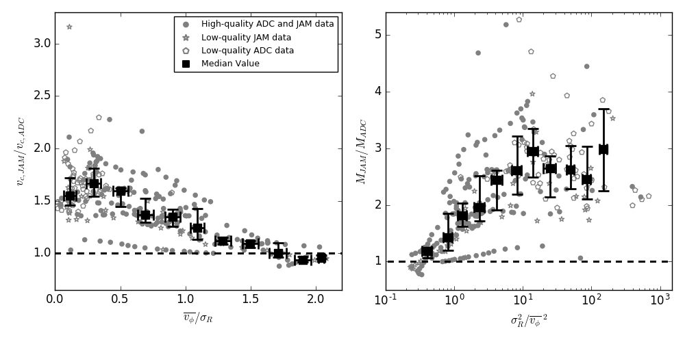
Figure 5: Velocity and mass ratios of the two models. The grey filled circles correspond to the velocity and mass ratios of high-quality ADC and JAM model fits data, while the open pentagon and the open star correspond to low-quality ADC and JAM data, respectively. The black filled squares show the median of the distribution of the data per bin with error bar corresponding to the uncertainties at the 25th and 75th percentiles. Left: The ordered-over-random motion $\overline{v_{\phi}}/\sigma_{R}$ (from the deprojected rotation and radial velocity dispersion profiles) as derived at different radii versus the velocity ratio $v_{c,\mathrm{JAM}}/v_{c,\mathrm{ADC}}$ at the same radii. The discrepancy between the ADC and JAM velocities becomes gradually larger for decreasing $\overline{v_{\phi}}/\sigma_{R}$ $\lesssim 1.5$, consistent with the presence of a dynamically hot bulge in the inner parts and/or a dynamically hot(ter) and thick(er) disc in the latest-type spiral galaxies. Right: The ratio $\sigma^{2}_{R}/\overline{v_{\phi}}^{2}$ (from the radial velocity dispersion profiles and deprojected rotation) as measured at different radii versus the mass ratio $M_{\mathrm{JAM}}/M_{\mathrm{ADC}}$ at the same radii. The discrepancy between the ADC and JAM inferred enclosed masses becomes gradually larger for increasing $\sigma^{2}_{R}/\overline{v_{\phi}}^{2}$, which has the same order of magnitude as the expected error in the epicycle approximation by Vandervoort (1975).

The differences we found between the circular velocity curves from the two modelling approaches can have a strong impact on the inferred total mass distribution and thus also on any follow-up inference like the amount of dark matter in the inner parts of these late-type spiral galaxies. We list the different assumptions adopted in both the axisymmetric Jeans models (JAM) and the asymmetric drift correction (ADC), and discuss the possible reasons for their discrepancy.

6 Discussion

6.1 Assumptions in the mass models

Mass-follows-light (JAM): Within the small radial range covered by the stellar kinematics, typically at $<R_{e}/3$, we expect the variations in the mass-to-light ratio to be small. Kent (1986) provides evidence that in a sample of 37 Sb-Sc galaxies, most of their rotation curves computes from the luminosity profiles assuming constant mass-to-light ratio provide a good match to the observed curve out to the radius where the predicted curve turns over. Additionally, Kregel & van der Kruit (2005) investigate the effects of realistic radially varying mass-to-light ratios and find the overall effect to only be $\sim$ 10% variations on the derived kinematic properties within $R_{e}/2$.

Constant anisotropy in the meridional plane (JAM): Whereas the velocity anisotropy $\sigma_{\phi}/\sigma_{R}$ in the equatorial plane is inherent in the solution of the axisymmetric Jeans equations (Section 3.1), the velocity anisotropy $\sigma_{z}/\sigma_{R}$ in the meridional plane is a free parameter, given as $\beta_{z}=1-\sigma^{2}_{z}/\sigma^{2}_{R}$. There is little evidence for strong variation of $\beta_{z}$. For example, Bottema (1993) already argued that for spirals the $\sigma_{z}/\sigma_{R}$ is constant at approximately 0.6, close to the measured value of $0.53\pm 0.07$ in the solar neighbourhood (Dehnen & Binney, 1998; Mignard, 2000). This ratio of the anisotropy is measured in a few spirals of type Sa to Sbc (Gerssen, Kuijken & Merrifield, 1997, 2000; Shapiro, Gerssen & van der Marel, 2003), yielding slightly larger constant values between 0.6 and 0.8. Based on long-slit spectra for a sample of 17 edge-on Sb–Scd spirals, Kregel & van der Kruit (2005) also adopt constant values, although slightly lower: 0.5 to 0.7. While radial variation of the anisotropy is not excluded, a constant value of $\beta_{z}$ should be sufficient for our analysis.

Shape of the velocity ellipsoid (JAM, ADC): The ADC and JAM models in our study assume that the velocity ellipsoid in the meridional plane is aligned with the cylindrical coordinate system so that $\overline{v_{R}v_{z}}=0$. Additionally, the ADC approach may allow for a tilt of the velocity ellipsoid through the parameter $\kappa$ having intermediate values between $\kappa=0$ and $\kappa=1$, corresponding to the cylindrical and spherical coordinate system, respectively. However, we expect that the resulting circular velocity curve is only weakly dependent on this tilt, because most of the stellar mass is concentrated toward the equatorial plane, particularly for late-type spiral galaxies. In that case, the assumption of axisymmetry gives $\overline{v_{R}v_{z}}=0$.

Dust (JAM, ADC): The surface brightness distribution of the spiral galaxies that is used in both JAM and ADC modelling approaches can be strongly affected by extinction due to dust. We have tried to minimise the effects of dust in various ways (G09): (i) selecting galaxies with intermediate inclinations so that they are not edge-on (where dust extinction is strongest) or face-on (where the stellar velocity dispersion would be significantly below the spectral resolution), (ii) inferring the surface brightness distribution from images in the near-infrared where the extinction is significantly smaller than in the optical, and (iii) fitting smooth, analytical MGE profiles to the radial surface brightness profile after azimuthally averaging over annuli to suppress deviations caused by bars, spiral arms, and regions obscured by dust. The stellar kinematics are obtained from integral-field spectroscopy in the optical and thus could also be affected if the (giant) stars that contribute along the line-of-sight with different motions are affected by the dust in different ways. For example, if dynamically colder stars closer to the disc plane are relatively more obscured than dynamically hotter stars above the disc plane, the resulting combined ordered-over-random motion could be biased to lower values. The effects of dust are strongly reduced for lines of sight only a few degrees away from edge-on (Baes et al. 2003) and the effects of extinction on the line-of-sight velocity are negligible: the change in $\sigma_{z}$ is only 1.3% higher from the dustless case (Bershady et al. 2010). Given the selection in our sample, the effects of dust on the inferred circular velocity curves from both modelling approaches are expected to be minimal.

Thin-disc (ADC): Circular velocity curves of spirals nearly always come from (cold) gas, which is naturally in a thin disc. The stellar discs of these late-type spiral galaxies are also believed to be thin, with inferred intrinsic flattening $q\sim 0.14$ (e.g., Kregel, van der Kruit & de Grijs, 2002). Even the bulges in late-type spiral galaxies are different from the ’classical’ bulges in lenticular galaxies. Sérsic profile fits to their surface brightness ($I(R)\propto\exp(-R^{1/n})$) show that towards later-types, the bulges are smaller in size, have profiles closer to exponential ($n=1$) than de Vaucouleurs ($n=4$), and are flatter (e.g., G09). Hence, the thin-disc assumption adopted in the ADC approach also seems to be reasonable.

6.2 Bulges and thick discs

Independent of the nature of the dynamically hot stellar (sub)system, it seems that the local value of the ordered-over-random motion is the key for understanding of the ADC and JAM discrepancy.

To explore that, in Fig. 4, we plot the radial velocity ratio $v_{\mathrm{c,JAM}}/v_{\mathrm{c,ADC}}$ of the galaxies, as well as the local luminosity fraction of the fitted exponential disc compared to the total luminosity as a thin solid curve. For the Sb–Sbc galaxies, the discrepancy in the estimated velocity ratio between the JAM and ADC models seems to be larger in the inner parts ($R<R_{e}/5$), where the luminosity is dominated by the presence of the bulge, and decreases outwards. For Scd–Sd galaxies the velocity ratio stays roughly constant and in a few cases increases towards larger radii, which could be due to the presence of a thick(er) disc component.

In the left panel of Fig. 5, we plot the velocity ratios $v_{\mathrm{c,JAM}}/v_{\mathrm{c,ADC}}$ obtained from Fig.4 for all galaxies as measured at different radii versus the ordered-over-random motion $\overline{v_{\phi}}/\sigma_{R}$ (the deprojected rotation vs. radial velocity dispersion) at the same radii. In the right panel of Fig. 5, we also show the ratio $\sigma^{2}_{R}/\overline{v_{\phi}}^{2}$ (from the radial velocity dispersion profiles and deprojected rotation) as measured at different radii versus the mass ratio $M_{\mathrm{JAM}}/M_{\mathrm{ADC}}=v_{c,\mathrm{JAM}}^{2}/v_{c,\mathrm{ADC}}^{2}$ at the same radii. The discrepancy between the ADC and JAM inferred enclosed masses becomes gradually larger for increasing $\sigma^{2}_{R}/\overline{v_{\phi}}^{2}$. The impact of the models’ discrepancy is larger when is converted into mass ratio. It also has the same order of magnitude as the expected uncertainty of the epicycle approximation ($\Delta\sim\sigma^{2}_{R}/\overline{v_{\phi}}^{2}$, Vandervoort 1975), which is actually applied in ADC (but not in JAM) approach.

We see that the circular velocity measurement of both modelling approaches are consistent for $\overline{v_{\phi}}/\sigma_{R}$ $\gtrsim 1.5$, corresponding to those radii in the Sb–Sbc galaxies where the disc luminosity is dominating over the bulge luminosity, i.e., where the thin solid curve in Fig. 4 approaches unity.

Since some of our galaxies do not have well fitting models, we mark their data with a different symbol in order to check for possible biases. However, even after their removal, the general trends of the velocity and mass ratios are preserved. The grey filled circles correspond to high-quality ADC and JAM model fits data, while the open pentagon and the open star correspond to low-quality ADC and JAM data, respectively. The black filled squares show the median of the distribution of the data per bin. The error bar corresponds to the uncertainties of the median value at the 25th and 75th percentiles of the distribution at each bin (see also Table 4).

Table 4: Median values of the velocity and mass ratios with corresponding (25th and 75th percentile) uncertainties at each bin in Fig.5: (1) Ratio between the deprojected rotation and radial velocity dispersion; (2) Velocity ratio between JAM and ADC model and their uncertainty at fixed $\overline{v_{\phi}}/\sigma_{R}$ ratio; (3) Ratio between the deprojected velocity and radial velocity dispersion; (4) Mass ratio between JAM and ADC model and their uncertainty at fixed $\sigma^{2}_{R}/\overline{v_{\phi}}^{2}$ ratio;

JAM-ADC conversion factors
$\overline{v_{\phi}}/\sigma_{R}$	$\frac{v_{\mathrm{c,JAM}}}{v_{\mathrm{c,ADC}}}$	$\sigma^{2}_{R}/\overline{v_{\phi}}^{2}$	$\frac{M_{\mathrm{JAM}}}{M_{\mathrm{ADC}}}$
(1)	(2)	(3)	(4)
0.1	$1.550_{-0.089}^{+0.168}$	0.4	$1.187_{-0.123}^{+0.055}$
0.3	$1.666_{-0.123}^{+0.147}$	0.8	$1.425_{-0.224}^{+0.424}$
0.5	$1.593_{-0.146}^{+0.025}$	1.3	$1.809_{-0.184}^{+0.227}$
0.7	$1.370_{-0.073}^{+0.157}$	2.4	$1.959_{-0.243}^{+0.551}$
0.9	$1.345_{-0.089}^{+0.072}$	4.2	$2.446_{-0.536}^{+0.162}$
1.1	$1.244_{-0.112}^{+0.184}$	8.3	$2.606_{-0.414}^{+0.603}$
1.3	$1.116_{-0.031}^{+0.033}$	14.1	$2.948_{-0.455}^{+0.404}$
1.5	$1.090_{-0.036}^{+0.026}$	24.8	$2.648_{-0.504}^{+0.215}$
1.7	$1.004_{-0.044}^{+0.092}$	49.6	$2.627_{-0.349}^{+0.414}$
1.9	$0.933_{-0.020}^{+0.037}$	85.5	$2.448_{-0.347}^{+0.582}$
2.0	$0.953_{-0.007}^{+0.030}$	150.1	$2.982_{-0.730}^{+0.719}$

Since we are probing the inner parts of these spiral galaxies it might well be the presence of bulges and/or thick stellar discs that causes a break-down of the thin-disc/epicycle approximation in ADC. As can be seen from Fig. 3, the stellar rotation (first column) is of the same order and often even lower than the stellar dispersion (second column). The small ordered-over-random motion values implies that the stars are far from dynamically cold.

Detailed photometric studies indicate that most disc galaxies contain a thick disc (e.g. Dalcanton & Bernstein, 2002; Seth, Dalcanton & de Jong, 2005; Comerón et al., 2011), and in low-mass galaxies with circular velocities $<$ 120 km s^-1, like the Scd–Sd galaxies in this sample, thick disc stars can contribute nearly half the luminosity and dominate the stellar mass (Yoachim & Dalcanton 2006). Moreover, recent hydrodynamical simulations that reproduce thick discs show that their typical scale lengths are around 3–5 kpc (e.g. Doménech-Moral et al., 2012), i.e., twice range typically covered by our analysis. Additionally, various earlier studies have qualitatively indicated that the ADC approach might not be suitable in the case of stellar systems that are (locally) not dynamically cold (e.g., Neistein et al., 1999; Bedregal, Aragón-Salamanca & Merrifield, 2006; Williams, Bureau & Cappellari, 2010). We also find that the discrepancy between the two model is proportional to the error of the epicycle approximation in ADC (see Vandervoort 1975), where $\sigma^{2}_{R}/\overline{v_{\phi}}^{2}\sim M_{\mathrm{JAM}}/M_{\mathrm{ADC}}$.

Davis et al. (2013) show that rotation curves of early-type galaxies based on the dynamically cold molecular gas are well traced by the $v_{c,\mathrm{JAM}}$, and that the $H_{\beta}/\mathrm{OIII}$ rotation curves from their SAURON data exhibit noticeable asymmetric drift. They also find the correction of the stellar rotation curve using ADC approach is also consistent with $v_{c,\mathrm{JAM}}$. However, they note that there is some indication that this becomes less true as velocity dispersion approaches the rotation speed, as we find in this study. It is not excluded that there are strong streaming motions in the centers of the SAURON galaxies due to presence of non-axisymmetric features, which prevent an accurate asymmetric-drft correction.

Nevertheless, some of the discrepancy might be arise from JAM overestimation of the M/L ratio. Lablanche et al. (2012) showed that the overestimation can be severe in face-on barred system. Davis et al. (2013) also discussed the possibility of an overestimation of the $M/L$ ratio due to disk averaging over various stellar populations. We do not exclude the latter since the region probed by our data is in the central part of the galaxies, where multiple stellar populations can be present. The former case should not influence some of our measurements, since all of our galaxies have intermediate inclinations.

In future studies, we will explore further this problem using large statistical sample of galaxies and morphologies.

7 Summary

The rotation curves of spiral galaxies, traced by atomic gas, provide the most direct path to estimate the total galaxy masses outside the stellar disc. However, it is not straightforward to measure the rotation curve in the central parts of the galaxies, where the ionized and molecular gas dominate. Gas settles in the equatorial or polar plane and is thus less sensitive to the mass distribution perpendicular to it. Gas is also dissipative and easily disturbed by perturbations in the plane from features like bars or spiral arms. Thus, stars appear to be a better tracer as they are distributed in all three dimensions and, being collisionless, they are less sensitive to perturbations. However, stars are not cold tracers as they move in orbits that are neither circular nor confined to a single plane. We therefore need to measure both velocity dispersions and line-of-sight velocities to recover the total mass distribution of galaxies.

In this paper we compare two different approaches for inferring dynamical masses of spiral galaxies: the commonly used asymmetric drift correction (ADC) and the axisymmetric Jeans equations. We used the stellar kinematics derived by integral field spectroscopy of a sample of 18 Sb – Sd galaxies, observed with the SAURON spectrograph. We obtained stellar mean velocity and velocity dispersion maps and derived the galaxies’ circular velocity curves by fitting solutions to the Jeans equations. Using the same data we also derived the circular velocity curves via the ADC technique. We use Markov Chain Monte Carlo methods to determine credible values for model parameters and their associated uncertainties.

The ADC approach gives systematically lower values than JAM for the circular velocity curves, and hence the enclosed mass, when $\overline{v_{\phi}}/\sigma_{R}$ $\lesssim 1.5$. The velocity ratio $v_{c,\mathrm{JAM}}/v_{c,\mathrm{ADC}}$ for Sb–Sbc galaxies is larger in the inner parts ($R<R_{e}/5$) and decreases outwards. However, for Scd–Sd galaxies the mass ratio stays roughly constant and in a few cases increases towards larger radii.

The complete Python codes, implementing MCMC analysis on both JAM and ADC models, described in this paper, can be downloaded from https://github.com/Kalinova/Dyn_models. These codes provide a robust way to estimate the uncertainties in the derived mass distribution of galaxies through their circular velocity curves.

Appendix A MGE Models

Here we provide a table with the parameters of our MGE models for each galaxy, where $I_{0,j}$ is the central surface brightness, $\xi^{\prime}_{j}$ is the the dispersion along the major $x^{\prime}$-axis, and $q^{\prime}_{j}$ is the flattening. Additionally, ind indicates the gaussians of the central, bulge or disc component of the galaxies with respective values of 0,1 and 2.

$j$	$I_{0,j}$	$\xi^{\prime}_{j}$	$q^{\prime}_{j}$	ind	$I_{0,j}$	$\xi^{\prime}_{j}$	$q^{\prime}_{j}$	ind	$I_{0,j}$	$\xi^{\prime}_{j}$	$q^{\prime}_{j}$	ind
	(L⊙ pc${}^{-2})$	(arcsec)			(L⊙ pc${}^{-2})$	(arcsec)			(L⊙ pc${}^{-2})$	(arcsec)
	NGC1042				NGC2805				NGC2964
1	29277.46	0.23	1.000	0	12769.80	0.12	1.000	0	78000.01	0.20	1.000	0
2	23.49	0.11	0.950	1	96.40	0.10	0.800	1	2617.84	0.10	0.950	1
3	54.40	0.26	0.950	1	134.25	0.24	0.800	1	4856.21	0.20	0.950	1
4	111.36	0.54	0.950	1	177.19	0.51	0.800	1	7703.26	0.35	0.950	1
5	200.80	1.00	0.950	1	213.89	1.01	0.800	1	10286.09	0.53	0.950	1
6	305.64	1.67	0.950	1	229.57	1.88	0.800	1	10381.19	0.74	0.950	1
7	361.53	2.53	0.950	1	212.94	3.31	0.800	1	6767.80	0.98	0.950	1
8	301.09	3.54	0.950	1	165.32	5.52	0.800	1	2380.00	1.23	0.950	1
9	162.48	4.62	0.950	1	103.93	8.75	0.800	1	379.76	1.48	0.950	1
10	51.72	5.76	0.950	1	51.22	13.28	0.800	1	24.00	1.73	0.950	1
11	7.95	6.98	0.950	1	19.17	19.38	0.800	1	0.54	1.98	0.950	1
12	0.15	7.97	0.950	1	5.24	27.40	0.800	1	0.00	2.24	0.950	1
13	0.32	8.37	0.950	1	0.98	37.78	0.800	1	0.00	2.52	0.950	1
14	0.00	9.78	0.950	1	0.12	51.15	0.800	1	0.00	17.76	0.950	1
15	0.00	11.44	0.950	1	0.01	68.32	0.800	1	343.25	1.00	0.550	2
16	0.00	23.70	0.950	1	0.00	90.34	0.800	1	847.42	4.13	0.550	2
17	0.00	77.53	0.950	1	0.00	118.84	0.800	1	1253.73	10.52	0.550	2
18	5.20	0.60	0.710	2	0.00	157.50	0.800	1	996.24	20.19	0.550	2
19	14.74	2.50	0.710	2	0.00	560.32	0.800	1	374.58	32.24	0.550	2
20	32.41	7.13	0.710	2	0.00	588.15	0.800	1	61.23	45.79	0.550	2
21	57.25	16.36	0.710	2	2.97	0.62	0.760	2	4.04	60.39	0.550	2
22	77.62	31.83	0.710	2	8.35	2.55	0.760	2	0.09	76.14	0.550	2
23	73.91	54.04	0.710	2	18.29	7.25	0.760	2	0.00	93.57	0.550	2
24	44.78	82.45	0.710	2	31.88	16.58	0.760	2	0.00	114.06	0.550	2
25	15.40	116.63	0.710	2	41.75	32.02	0.760	2	…	…	…	…
26	2.41	157.63	0.710	2	37.57	53.88	0.760	2	…	…	…	…
27	0.10	210.10	0.710	2	21.02	81.47	0.760	2	…	…	…	…
28	…	…	…	…	6.51	114.33	0.760	2	…	…	…	…
29	…	…	…	…	0.90	153.37	0.760	2	…	…	…	…
30	…	…	…	…	0.03	202.87	0.760	2	…	…	…	…
$j$	$I_{0,j}$	$\xi^{\prime}_{j}$	$q^{\prime}_{j}$	ind	$I_{0,j}$	$\xi^{\prime}_{j}$	$q^{\prime}_{j}$	ind	$I_{0,j}$	$\xi^{\prime}_{j}$	$q^{\prime}_{j}$	ind
	(L⊙ pc${}^{-2})$	(arcsec)			(L⊙ pc${}^{-2})$	(arcsec)			(L⊙ pc${}^{-2})$	(arcsec)
	NGC3346				NGC3423				NGC3949
1	8592.16	0.12	1.000	0	13792.68	0.12	1.000	0	33147.01	0.12	1.000	0
2	5.52	0.10	0.750	1	123.67	0.10	0.870	1	247.94	0.10	0.700	1
3	12.93	0.21	0.750	1	180.26	0.23	0.870	1	415.67	0.22	0.700	1
4	23.81	0.36	0.750	1	250.35	0.47	0.870	1	648.53	0.45	0.700	1
5	52.10	0.59	0.750	1	322.26	0.89	0.870	1	915.74	0.81	0.700	1
6	127.03	0.95	0.750	1	372.27	1.58	0.870	1	1122.66	1.37	0.700	1
7	257.57	1.47	0.750	1	374.59	2.64	0.870	1	1141.20	2.17	0.700	1
8	358.46	2.04	0.750	1	317.69	4.20	0.870	1	911.23	3.25	0.700	1
9	266.26	2.59	0.750	1	219.51	6.36	0.870	1	534.22	4.61	0.700	1
10	81.56	3.06	0.750	1	119.93	9.18	0.870	1	209.63	6.30	0.700	1
11	7.86	3.49	0.750	1	50.95	12.73	0.870	1	48.61	8.33	0.700	1
12	0.17	3.88	0.750	1	16.66	17.08	0.870	1	5.69	10.75	0.700	1
13	0.00	4.25	0.750	1	3.89	22.51	0.870	1	0.28	13.60	0.700	1
14	0.00	30.87	0.750	1	0.55	29.44	0.870	1	0.00	16.93	0.700	1
15	20.03	1.12	0.840	2	0.04	38.25	0.870	1	0.00	20.87	0.700	1
16	54.82	4.86	0.840	2	0.00	49.35	0.870	1	0.00	25.54	0.700	1
17	102.72	13.39	0.840	2	0.00	63.23	0.870	1	0.00	31.02	0.700	1
18	125.36	28.07	0.840	2	0.00	80.66	0.870	1	0.00	190.20	0.700	1
19	88.40	48.50	0.840	2	0.00	103.25	0.870	1	255.39	1.02	0.640	2
20	32.26	73.22	0.840	2	0.00	588.15	0.870	1	619.84	4.19	0.640	2
21	5.54	101.15	0.840	2	20.07	1.09	0.770	2	886.68	10.58	0.640	2
22	0.38	132.44	0.840	2	55.32	4.74	0.770	2	663.27	20.12	0.640	2
23	0.01	169.72	0.840	2	105.74	13.13	0.770	2	227.58	31.90	0.640	2
24	0.00	588.15	0.840	2	134.74	27.78	0.770	2	32.95	45.07	0.640	2
25	…	…	…	…	101.83	48.48	0.770	2	1.87	59.22	0.640	2
26	…	…	…	…	40.74	73.85	0.770	2	0.04	74.44	0.640	2
27	…	…	…	…	7.85	102.70	0.770	2	0.00	91.29	0.640	2
28	…	…	…	…	0.62	135.13	0.770	2	0.00	111.07	0.640	2
29	…	…	…	…	0.01	173.88	0.770	2	…	…	…	…
30	…	…	…	…	0.00	588.15	0.770	2	…	…	…	…

$j$	$I_{0,j}$	$\xi^{\prime}_{j}$	$q^{\prime}_{j}$	ind	$I_{0,j}$	$\xi^{\prime}_{j}$	$q^{\prime}_{j}$	ind	$I_{0,j}$	$\xi^{\prime}_{j}$	$q^{\prime}_{j}$	ind
	(L⊙ pc${}^{-2})$	(arcsec)			(L⊙ pc${}^{-2})$	(arcsec)			(L⊙ pc${}^{-2})$	(arcsec)
	NGC4030				NGC4102				NGC4254
1	48113.13	0.13	1.000	0	0.00	1.52	1.000	0	55276.68	0.21	1.000	0
2	6683.20	0.10	0.850	1	780479.16	0.10	0.800	1	2360.27	0.10	0.900	1
3	6306.38	0.23	0.850	1	430239.29	0.23	0.800	1	2650.37	0.23	0.900	1
4	5769.43	0.44	0.850	1	225993.57	0.44	0.800	1	2884.28	0.48	0.900	1
5	5280.87	0.77	0.850	1	105795.77	0.79	0.800	1	2932.75	0.93	0.900	1
6	4689.74	1.30	0.850	1	41165.86	1.37	0.800	1	2689.19	1.71	0.900	1
7	3905.92	2.13	0.850	1	12914.85	2.25	0.800	1	2177.31	2.97	0.900	1
8	2987.56	3.39	0.850	1	3209.39	3.58	0.800	1	1527.83	4.96	0.900	1
9	2069.12	5.26	0.850	1	623.15	5.52	0.800	1	912.72	7.94	0.900	1
10	1282.12	7.99	0.850	1	93.51	8.24	0.800	1	456.20	12.23	0.900	1
11	702.74	11.89	0.850	1	10.74	12.00	0.800	1	187.78	18.20	0.900	1
12	336.43	17.36	0.850	1	0.93	17.08	0.800	1	63.06	26.20	0.900	1
13	138.18	24.94	0.850	1	0.06	23.90	0.800	1	17.31	36.60	0.900	1
14	47.39	35.41	0.850	1	0.00	33.05	0.800	1	3.86	50.03	0.900	1
15	13.07	49.82	0.850	1	0.00	45.35	0.800	1	0.64	67.87	0.900	1
16	2.76	69.65	0.850	1	0.00	61.94	0.800	1	0.07	92.37	0.900	1
17	0.42	97.03	0.850	1	0.00	84.36	0.800	1	0.00	127.13	0.900	1
18	0.04	135.26	0.850	1	0.00	115.03	0.800	1	0.00	180.77	0.900	1
19	0.00	190.51	0.850	1	0.00	159.32	0.800	1	0.00	588.15	0.900	1
20	0.00	279.53	0.850	1	0.00	317.40	0.800	1	41.78	0.67	0.730	2
21	94.59	0.79	0.760	2	417.54	0.99	0.555	2	116.76	2.77	0.730	2
22	257.16	3.32	0.760	2	1034.48	4.11	0.555	2	247.55	7.80	0.730	2
23	490.15	9.09	0.760	2	1546.11	10.50	0.555	2	402.28	17.44	0.730	2
24	622.90	19.14	0.760	2	1252.87	20.20	0.555	2	465.56	32.71	0.730	2
25	471.99	33.32	0.760	2	484.60	32.33	0.555	2	345.32	53.37	0.730	2
26	190.98	50.64	0.760	2	82.09	46.01	0.555	2	148.27	78.49	0.730	2
27	37.79	70.24	0.760	2	5.66	60.77	0.555	2	32.87	107.57	0.730	2
28	3.26	91.86	0.760	2	0.14	76.67	0.555	2	3.02	141.30	0.730	2
29	0.10	116.04	0.760	2	0.00	94.30	0.555	2	0.07	183.07	0.730	2
30	0.00	144.89	0.760	2	0.00	115.01	0.555	2	…	…	…	…
$j$	$I_{0,j}$	$\xi^{\prime}_{j}$	$q^{\prime}_{j}$	ind	$I_{0,j}$	$\xi^{\prime}_{j}$	$q^{\prime}_{j}$	ind	$I_{0,j}$	$\xi^{\prime}_{j}$	$q^{\prime}_{j}$	ind
	(L⊙ pc${}^{-2})$	(arcsec)			(L⊙ pc${}^{-2})$	(arcsec)			(L⊙ pc${}^{-2})$	(arcsec)
	NGC4487				NGC4775				NGC0488
1	29433.24	0.17	1.000	0	21385.18	0.12	1.000	0	24161.14	0.38	1.000	0
2	128.29	0.11	0.600	1	85.94	0.12	0.830	1	16980.54	0.10	0.900	1
3	205.54	0.29	0.600	1	104.35	0.28	0.830	1	14945.13	0.23	0.900	1
4	289.40	0.67	0.600	1	70.83	0.43	0.830	1	12930.46	0.46	0.900	1
5	350.12	1.40	0.600	1	137.73	0.65	0.830	1	10797.95	0.84	0.900	1
6	338.21	2.63	0.600	1	156.92	0.98	0.830	1	8245.04	1.48	0.900	1
7	256.84	4.48	0.600	1	206.29	1.49	0.830	1	5595.02	2.53	0.900	1
8	154.95	6.99	0.600	1	231.29	2.26	0.830	1	3318.18	4.17	0.900	1
9	79.42	10.36	0.600	1	231.40	3.42	0.830	1	1694.88	6.66	0.900	1
10	27.00	14.96	0.600	1	176.99	5.18	0.830	1	734.89	10.33	0.900	1
11	6.26	20.87	0.600	1	86.68	7.85	0.830	1	266.76	15.61	0.900	1
12	0.82	28.64	0.600	1	18.69	11.90	0.830	1	79.95	23.02	0.900	1
13	0.05	38.42	0.600	1	0.96	18.03	0.830	1	19.44	33.25	0.900	1
14	0.00	50.53	0.600	1	0.00	27.32	0.830	1	3.72	47.28	0.900	1
15	0.00	65.51	0.600	1	0.00	41.39	0.830	1	0.53	66.51	0.900	1
16	0.00	84.25	0.600	1	0.00	62.71	0.830	1	0.05	93.11	0.900	1
17	0.00	108.71	0.600	1	0.00	330.56	0.830	1	0.00	130.94	0.900	1
18	0.00	588.15	0.600	1	50.98	0.92	0.865	2	0.00	189.04	0.900	1
19	21.17	1.08	0.630	2	131.09	3.83	0.865	2	0.00	307.69	0.900	1
20	58.35	4.71	0.630	2	216.63	10.04	0.865	2	0.00	323.27	0.900	1
21	111.87	13.06	0.630	2	209.75	19.96	0.865	2	30.42	0.69	0.770	2
22	143.33	27.67	0.630	2	104.72	32.85	0.865	2	84.00	2.87	0.770	2
23	109.17	48.36	0.630	2	24.46	47.73	0.865	2	176.60	8.01	0.770	2
24	44.17	73.72	0.630	2	2.48	64.00	0.865	2	287.49	17.80	0.770	2
25	8.66	102.54	0.630	2	0.10	81.62	0.865	2	340.68	33.29	0.770	2
26	0.71	134.83	0.630	2	0.00	101.14	0.865	2	267.03	54.34	0.770	2
27	0.02	173.29	0.630	2	0.00	124.14	0.865	2	125.56	80.14	0.770	2
28	0.00	588.15	0.630	2	…	…	…	…	31.53	110.27	0.770	2
29	…	…	…	…	…	…	…	…	3.38	145.59	0.770	2
30	…	…	…	…	…	…	…	…	0.09	189.76	0.770	2

$j$	$I_{0,j}$	$\xi^{\prime}_{j}$	$q^{\prime}_{j}$	ind	$I_{0,j}$	$\xi^{\prime}_{j}$	$q^{\prime}_{j}$	ind	$I_{0,j}$	$\xi^{\prime}_{j}$	$q^{\prime}_{j}$	ind
	(L⊙ pc${}^{-2})$	(arcsec)			(L⊙ pc${}^{-2})$	(arcsec)			(L⊙ pc${}^{-2})$	(arcsec)
	NGC5585				NGC5668				NGC5678
1	5628.53	0.27	1.000	0	10359.16	0.12	1.000	0	34754.46	0.32	1.000	0
2	4.28	0.12	0.800	1	86.95	0.10	0.800	1	25905.05	0.10	0.800	1
3	8.11	0.28	0.800	1	126.05	0.24	0.800	1	17168.58	0.22	0.800	1
4	1.55	0.43	0.800	1	173.70	0.51	0.800	1	12031.87	0.42	0.800	1
5	18.27	0.65	0.800	1	220.00	1.01	0.800	1	8529.89	0.76	0.800	1
6	5.84	0.98	0.800	1	249.90	1.89	0.800	1	4679.15	1.39	0.800	1
7	38.14	1.49	0.800	1	247.84	3.34	0.800	1	1949.35	2.47	0.800	1
8	23.61	2.26	0.800	1	207.79	5.58	0.800	1	629.79	4.20	0.800	1
9	72.02	3.42	0.800	1	142.25	8.86	0.800	1	156.65	6.86	0.800	1
10	70.47	5.18	0.800	1	76.86	13.45	0.800	1	29.61	10.81	0.800	1
11	112.16	7.85	0.800	1	31.67	19.61	0.800	1	4.21	16.44	0.800	1
12	95.48	11.90	0.800	1	9.54	27.69	0.800	1	0.45	24.24	0.800	1
13	45.38	18.03	0.800	1	1.97	38.11	0.800	1	0.04	34.80	0.800	1
14	3.29	27.32	0.800	1	0.25	51.47	0.800	1	0.00	48.82	0.800	1
15	0.00	41.39	0.800	1	0.02	68.50	0.800	1	0.00	67.20	0.800	1
16	0.00	62.71	0.800	1	0.00	90.18	0.800	1	0.00	90.83	0.800	1
17	0.00	330.56	0.800	1	0.00	117.92	0.800	1	0.00	121.04	0.800	1
18	3.22	0.59	0.640	2	0.00	154.81	0.800	1	0.00	164.61	0.800	1
19	9.10	2.43	0.640	2	0.00	588.15	0.800	1	0.00	309.03	0.800	1
20	20.23	6.96	0.640	2	10.14	0.75	0.845	2	0.00	588.15	0.800	1
21	36.28	16.06	0.640	2	27.94	3.13	0.845	2	168.11	0.89	0.525	2
22	50.54	31.49	0.640	2	55.57	8.68	0.845	2	439.46	3.72	0.525	2
23	50.21	53.94	0.640	2	77.06	18.68	0.845	2	749.06	9.87	0.525	2
24	32.24	82.97	0.640	2	67.35	33.27	0.845	2	769.26	19.83	0.525	2
25	11.93	118.18	0.640	2	33.11	51.61	0.845	2	418.84	32.99	0.525	2
26	2.05	160.73	0.640	2	8.34	72.73	0.845	2	109.35	48.32	0.525	2
27	0.09	215.52	0.640	2	0.96	96.26	0.845	2	12.68	65.17	0.525	2
28	…	…	…	…	0.04	122.79	0.845	2	0.57	83.47	0.525	2
29	…	…	…	…	0.00	154.70	0.845	2	0.01	103.77	0.525	2
30	…	…	…	…	…	…	…	…	0.00	127.71	0.525	2
$j$	$I_{0,j}$	$\xi^{\prime}_{j}$	$q^{\prime}_{j}$	ind	$I_{0,j}$	$\xi^{\prime}_{j}$	$q^{\prime}_{j}$	ind	$I_{0,j}$	$\xi^{\prime}_{j}$	$q^{\prime}_{j}$	ind
	(L⊙ pc${}^{-2})$	(arcsec)			(L⊙ pc${}^{-2})$	(arcsec)			(L⊙ pc${}^{-2})$	(arcsec)
	NGC0628				NGC0772				NGC0864
1	32854.43	0.16	1.000	0	96530.87	0.32	1.000	0	834.18	1.90	1.000	0
2	125.78	0.10	0.950	1	11343.60	0.10	0.830	1	26446.20	0.10	0.950	1
3	225.98	0.24	0.950	1	8973.63	0.23	0.830	1	12341.46	0.22	0.950	1
4	374.32	0.52	0.950	1	7132.09	0.46	0.830	1	6151.01	0.41	0.950	1
5	564.49	1.04	0.950	1	5671.02	0.85	0.830	1	3110.85	0.72	0.950	1
6	758.45	1.91	0.950	1	4271.96	1.50	0.830	1	1406.19	1.21	0.950	1
7	876.39	3.27	0.950	1	2958.77	2.58	0.830	1	526.61	2.02	0.950	1
8	831.86	5.26	0.950	1	1857.68	4.33	0.830	1	160.13	3.31	0.950	1
9	616.02	7.97	0.950	1	1046.19	7.08	0.830	1	38.78	5.33	0.950	1
10	336.16	11.49	0.950	1	523.09	11.31	0.830	1	7.30	8.43	0.950	1
11	125.58	15.89	0.950	1	229.91	17.66	0.830	1	1.05	13.08	0.950	1
12	28.95	21.29	0.950	1	88.03	27.01	0.830	1	0.11	19.87	0.950	1
13	3.59	27.84	0.950	1	29.12	40.50	0.830	1	0.01	29.56	0.950	1
14	0.20	35.71	0.950	1	8.24	59.73	0.830	1	0.00	43.04	0.950	1
15	0.00	45.12	0.950	1	1.95	87.17	0.830	1	0.00	61.32	0.950	1
16	0.00	56.40	0.950	1	0.37	127.32	0.830	1	0.00	85.89	0.950	1
17	0.00	70.00	0.950	1	0.05	190.42	0.830	1	0.00	120.15	0.950	1
18	0.00	86.58	0.950	1	0.00	307.88	0.830	1	0.00	173.33	0.950	1
19	0.00	489.20	0.950	1	0.00	587.78	0.830	1	0.00	303.66	0.950	1
20	9.91	0.57	0.810	2	20.98	0.65	0.660	2	0.00	588.15	0.950	1
21	28.13	2.32	0.810	2	58.45	2.67	0.660	2	49.80	0.77	0.680	2
22	63.36	6.67	0.810	2	125.53	7.53	0.660	2	137.00	3.23	0.680	2
23	117.06	15.56	0.810	2	212.58	16.98	0.660	2	265.67	8.90	0.680	2
24	173.22	30.99	0.810	2	268.28	32.34	0.660	2	352.74	18.92	0.680	2
25	190.87	54.10	0.810	2	228.94	53.78	0.660	2	287.21	33.30	0.680	2
26	143.02	84.87	0.810	2	119.18	80.57	0.660	2	128.14	51.11	0.680	2
27	65.22	123.15	0.810	2	33.60	112.23	0.660	2	28.60	71.43	0.680	2
28	14.54	170.51	0.810	2	4.11	149.61	0.660	2	2.85	93.96	0.680	2
29	0.89	232.94	0.810	2	0.12	196.62	0.660	2	0.10	119.25	0.680	2
30	…	…	…	…	…	…	…	…	0.00	149.53	0.680	2

Appendix B JAM-MCMC burn-in chains, posterior chains and corner plots

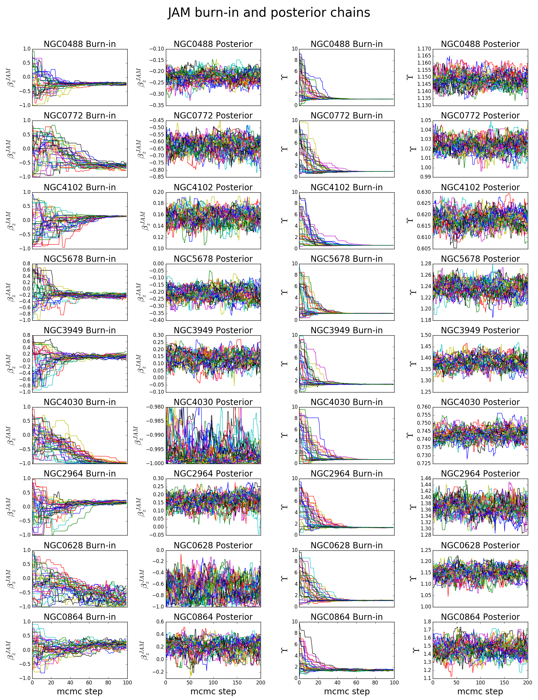
Figure 6: Burn-in and posterior chain plots of the velocity anisotropy ($\beta^{\mathrm{JAM}}_{z}$) and mass-to-light ratio ($\Upsilon$) in JAM-MCMC method.

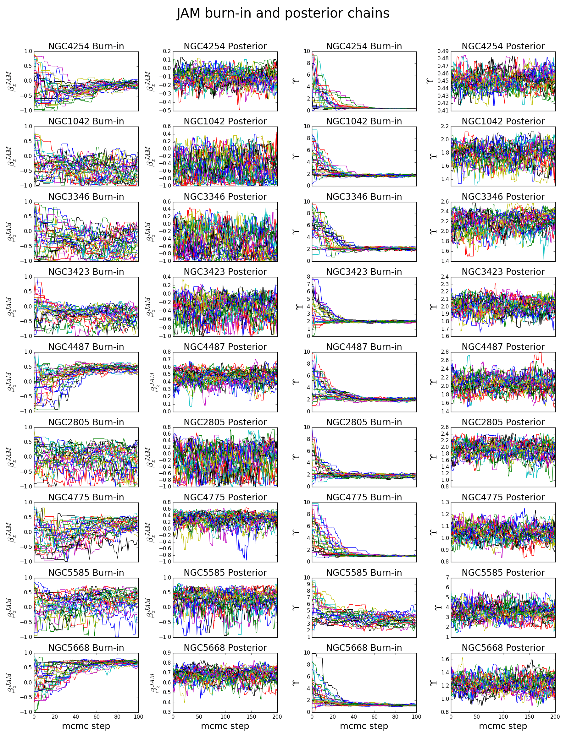
Figure 6: – continuation

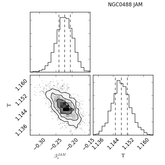
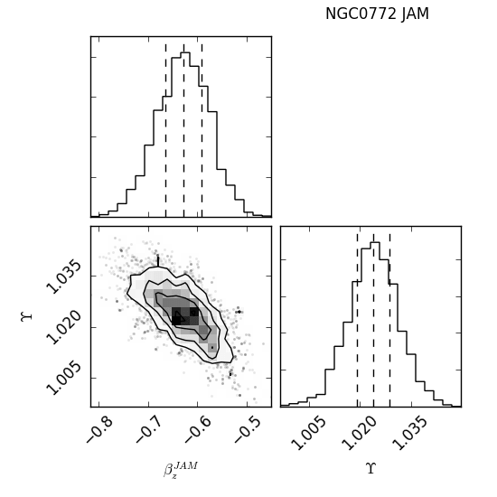
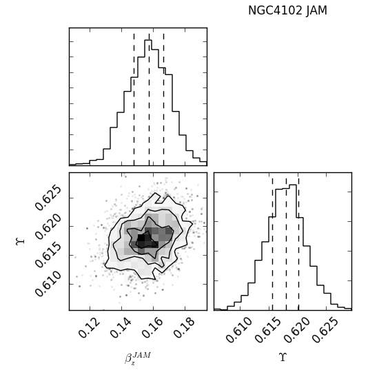
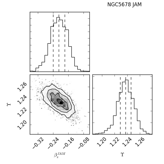
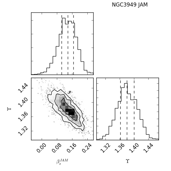
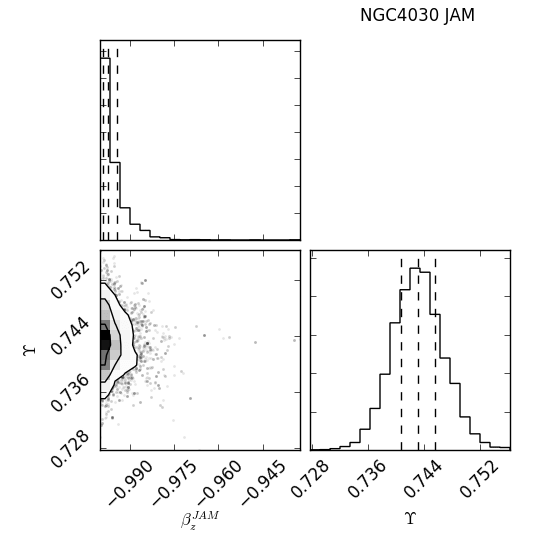
Figure 7: Corner plot that shows the covariance between the model parameters of the 18 galaxies from the JAM-MCMC method. Overplotted are the median value of the distributions related to the fitted parameters, together with their uncertainties at 25 and 75 percentiles.

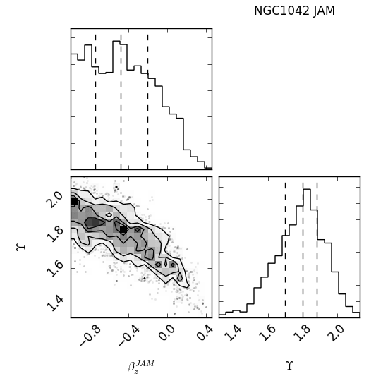
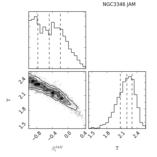
Figure 7: – continuation

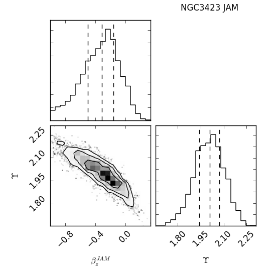
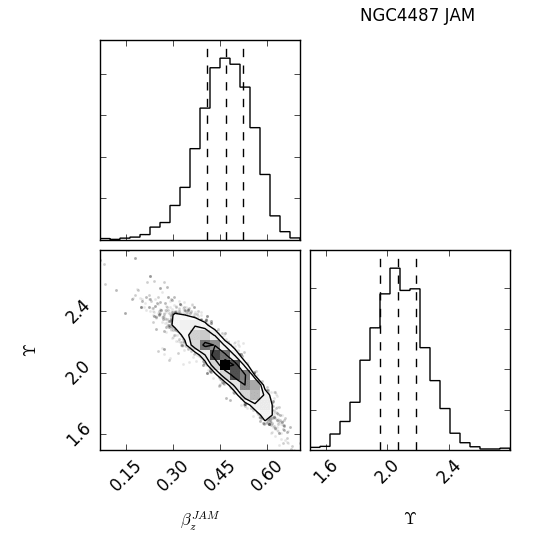
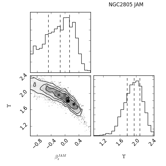
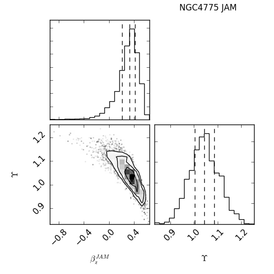
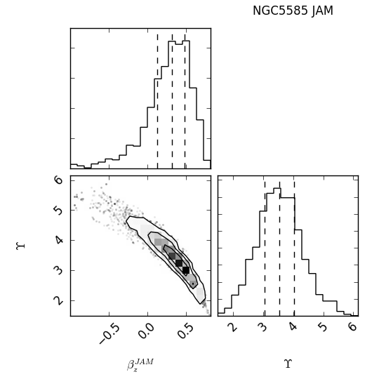
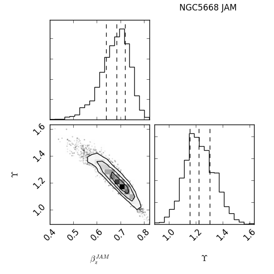
Figure 7: – continuation

Appendix C ADC-MCMC burn-in chains, posterior chains and corner plots

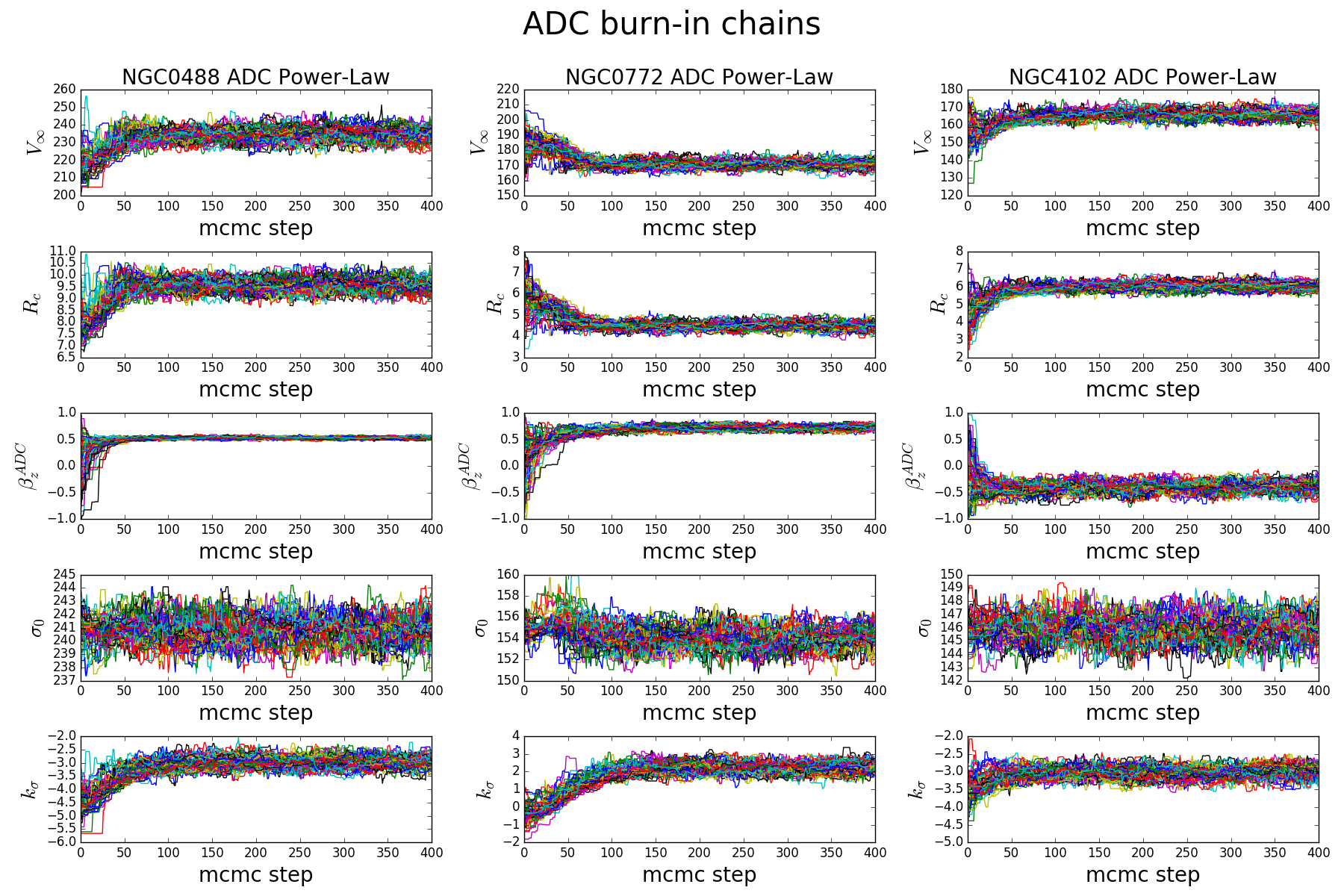
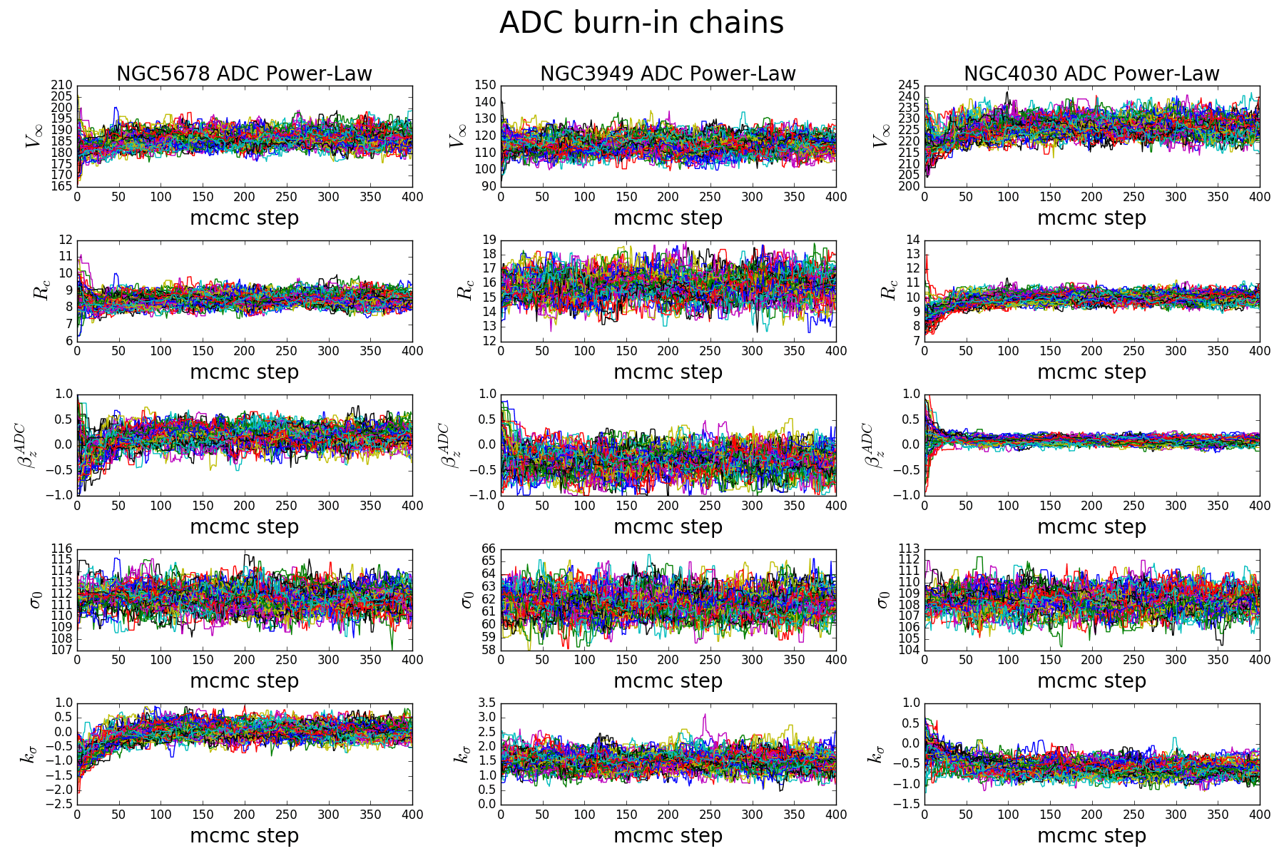
Figure 8: Burn-in chain plots of model parameters for the 18 galaxies from ADC-MCMC method.

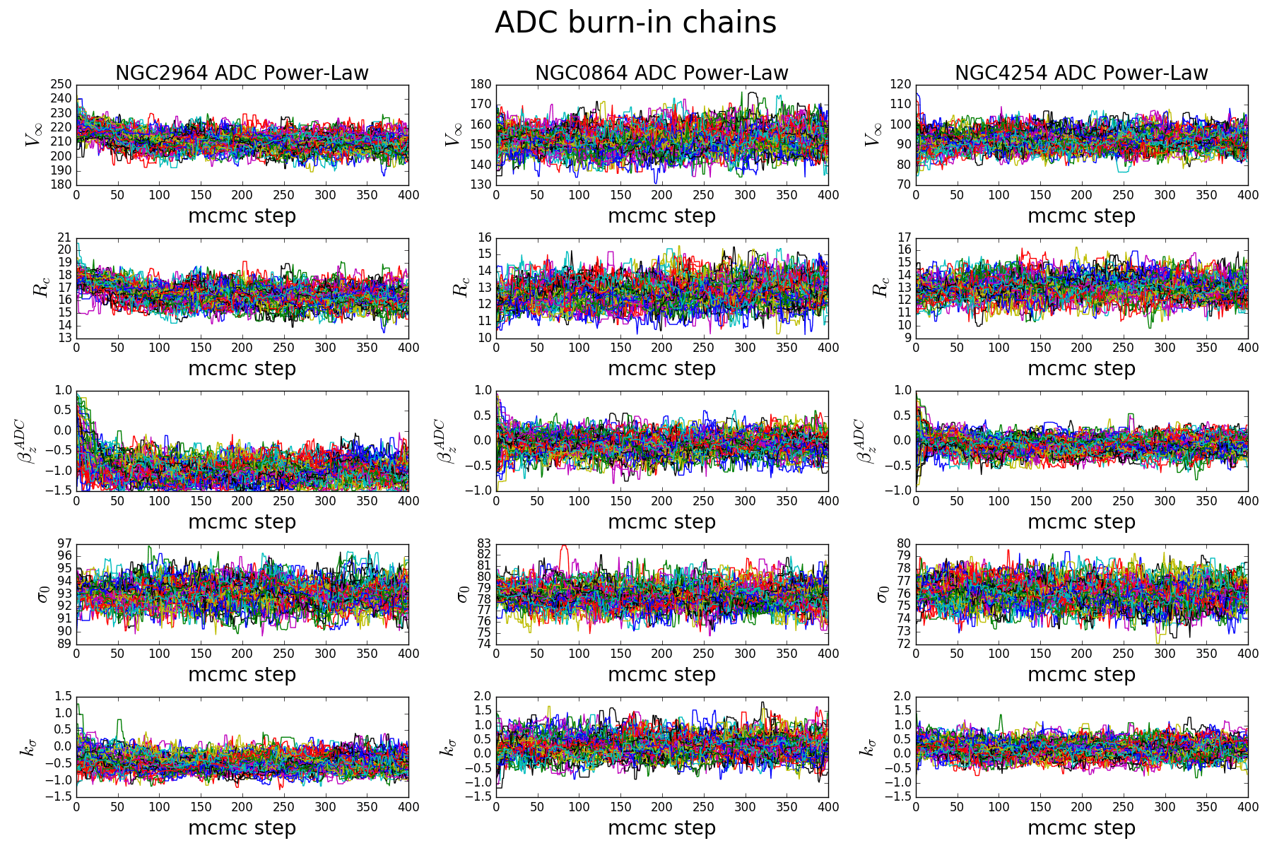
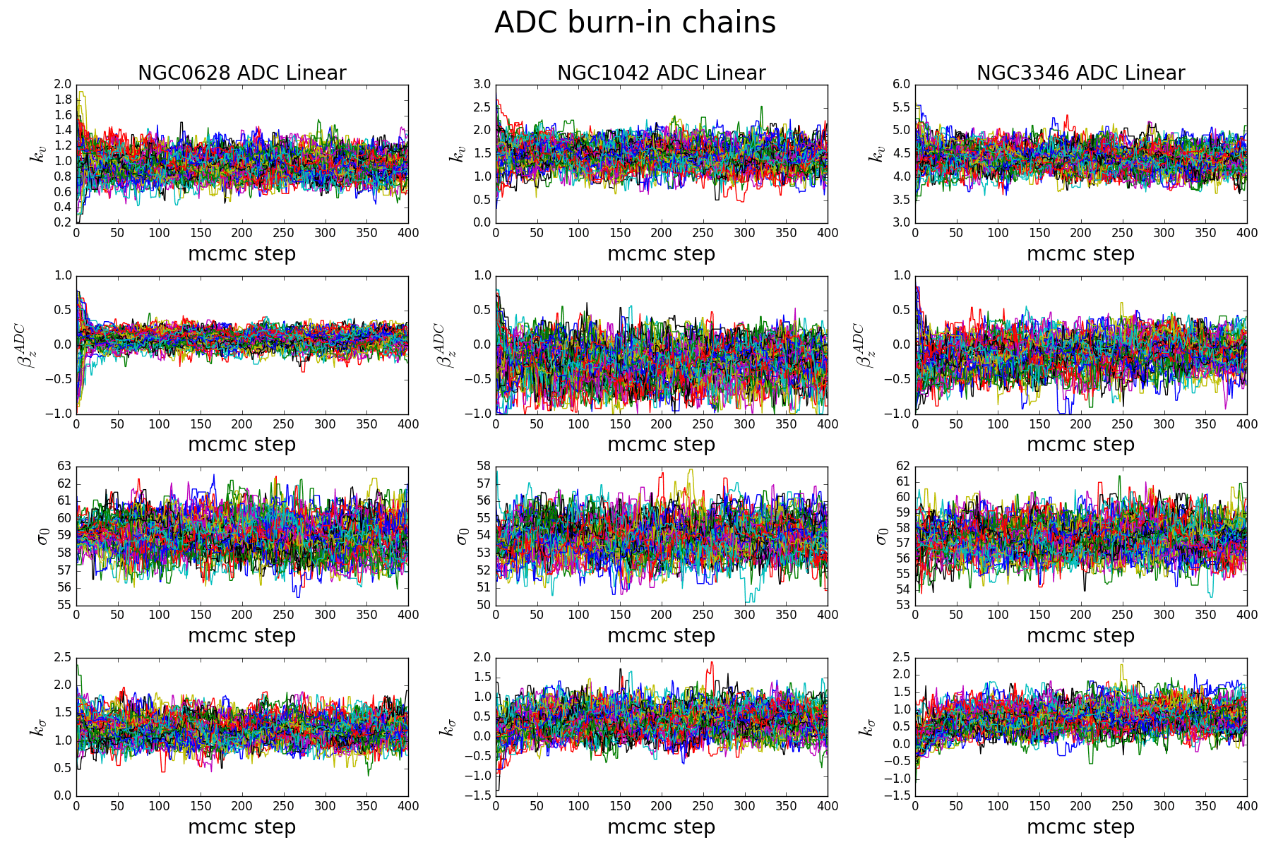
Figure 8: – continuation

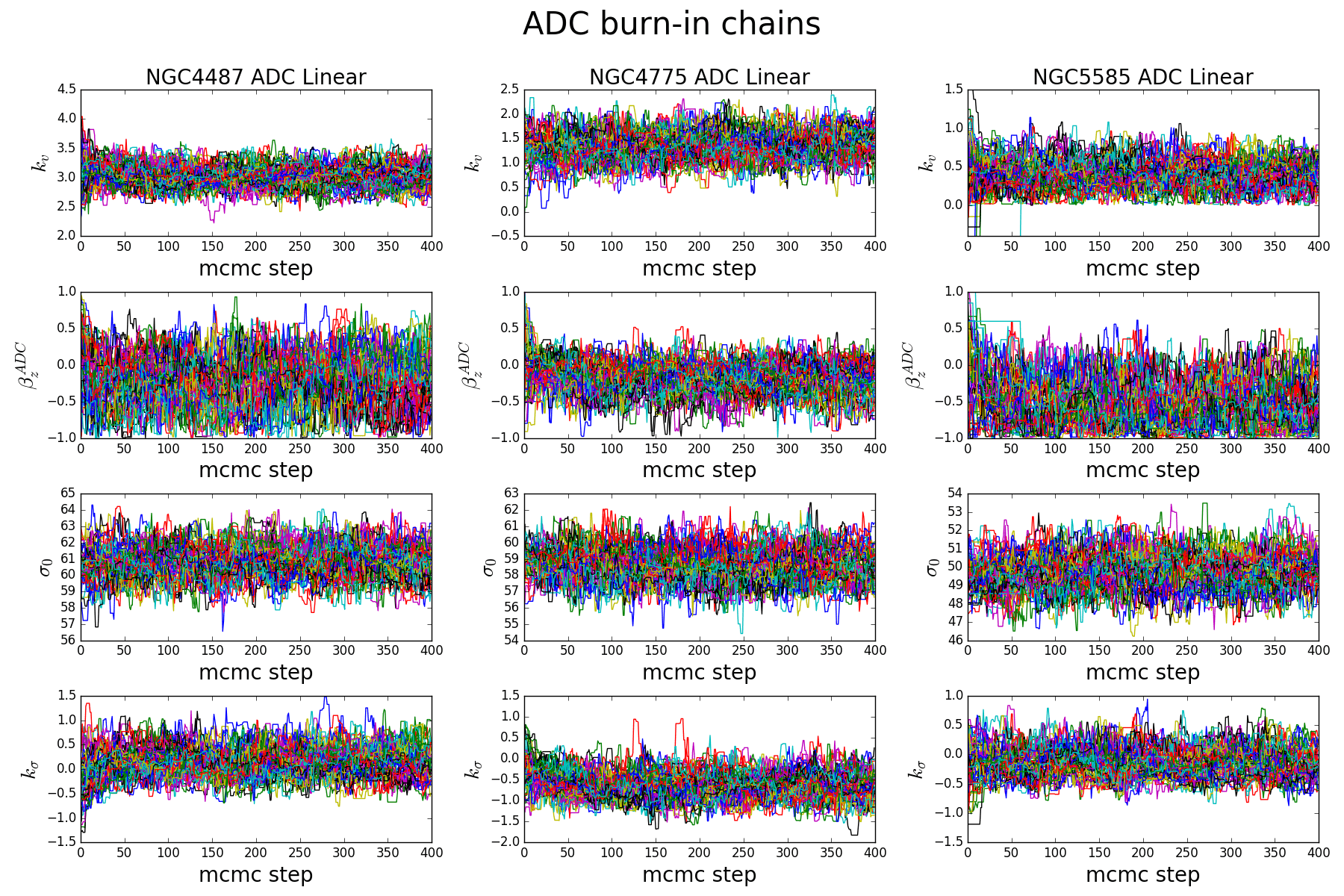
Figure 8: – continuation

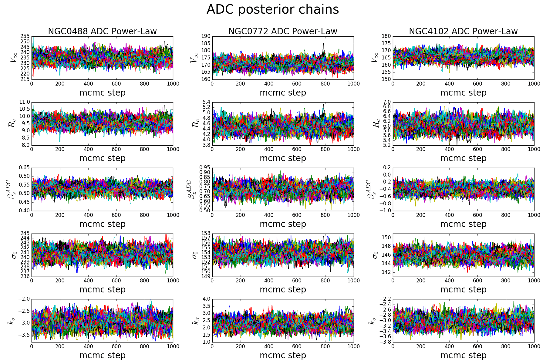
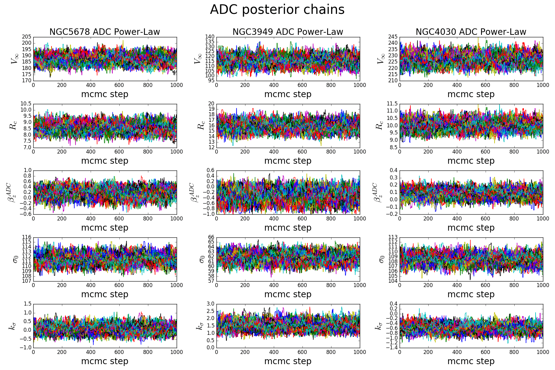
Figure 9: Posterior chain plots of model parameters for the 18 galaxies from ADC-MCMC method.

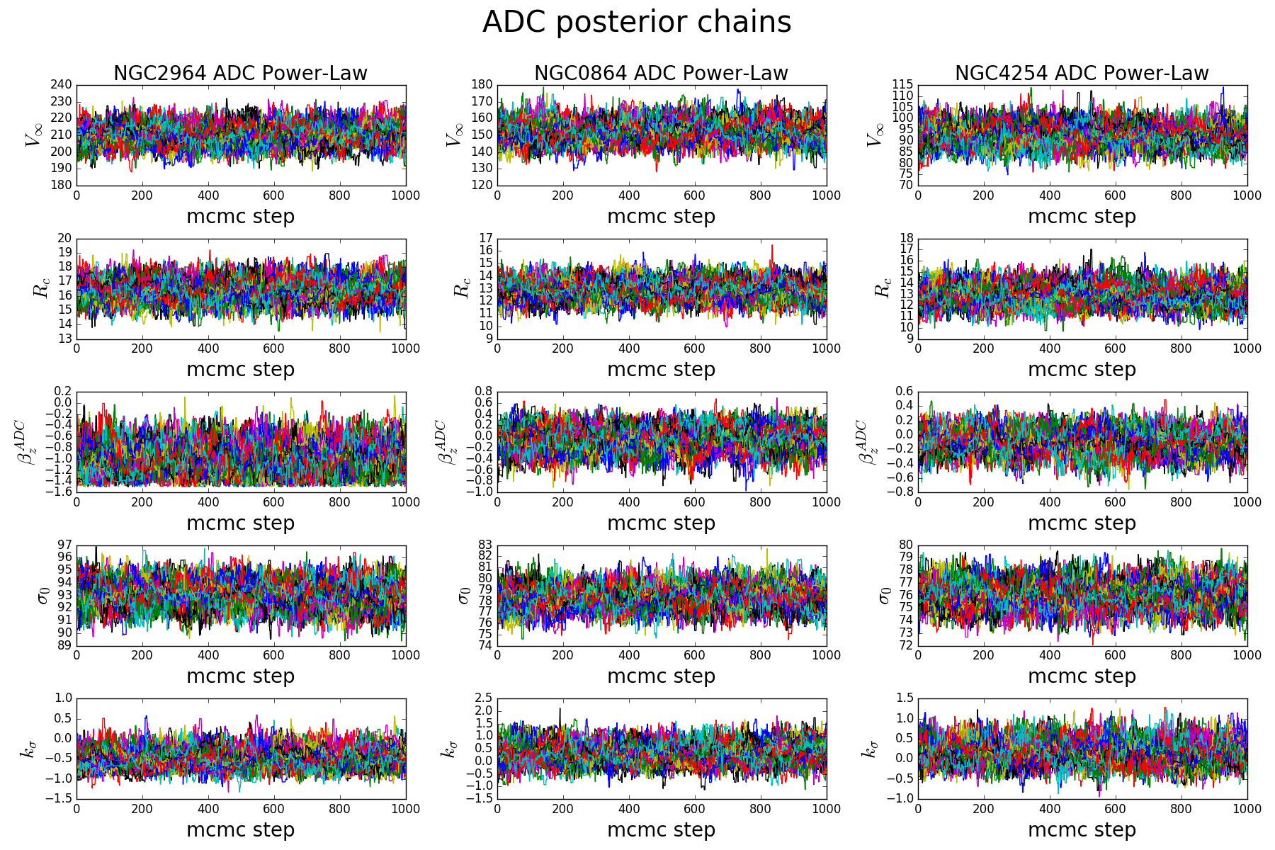
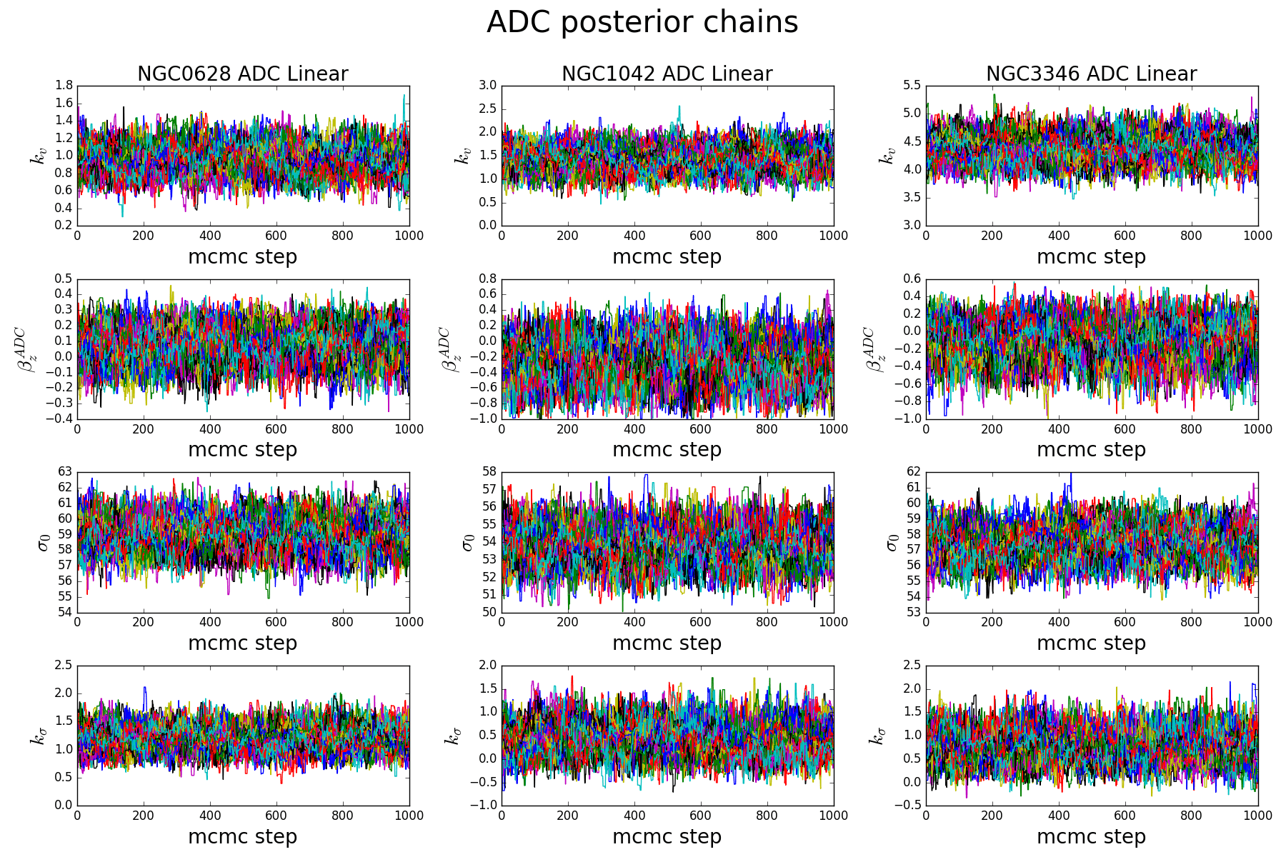
Figure 9: – continuation

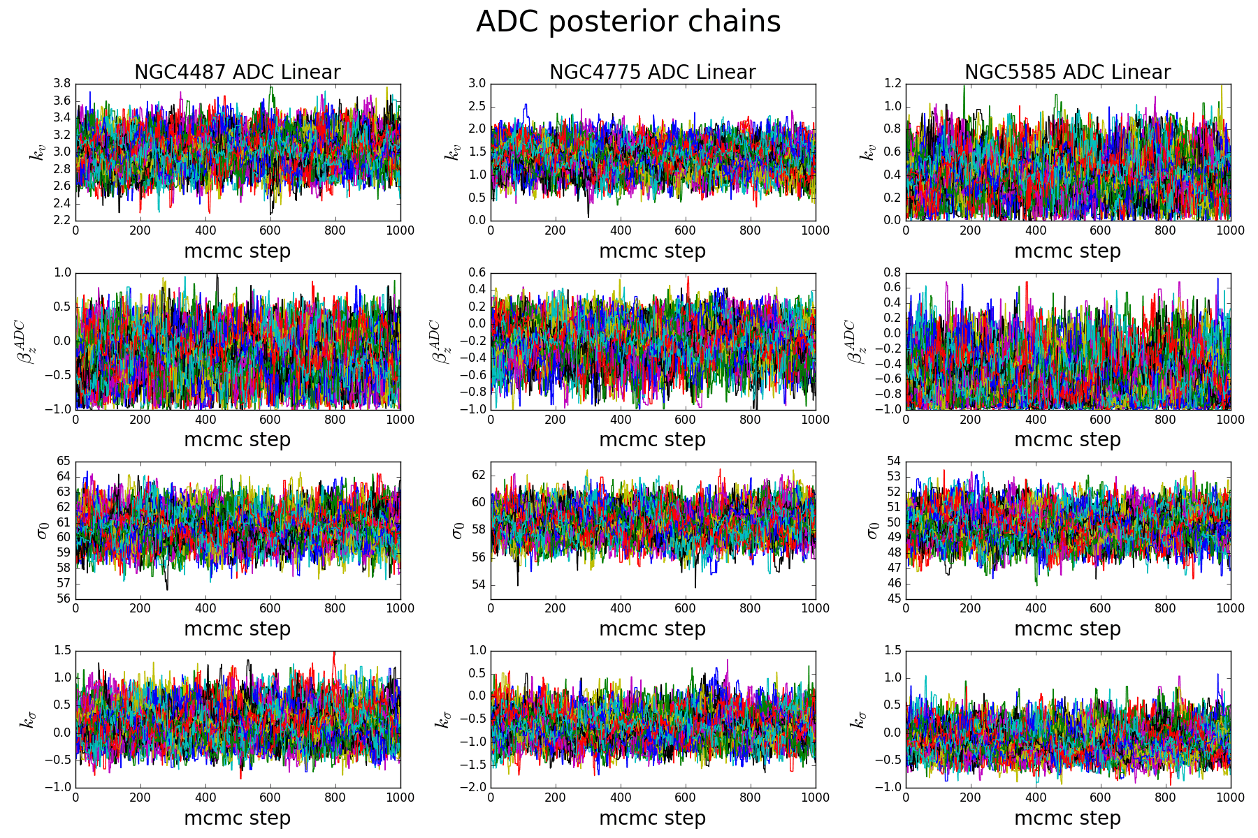
Figure 9: – continuation

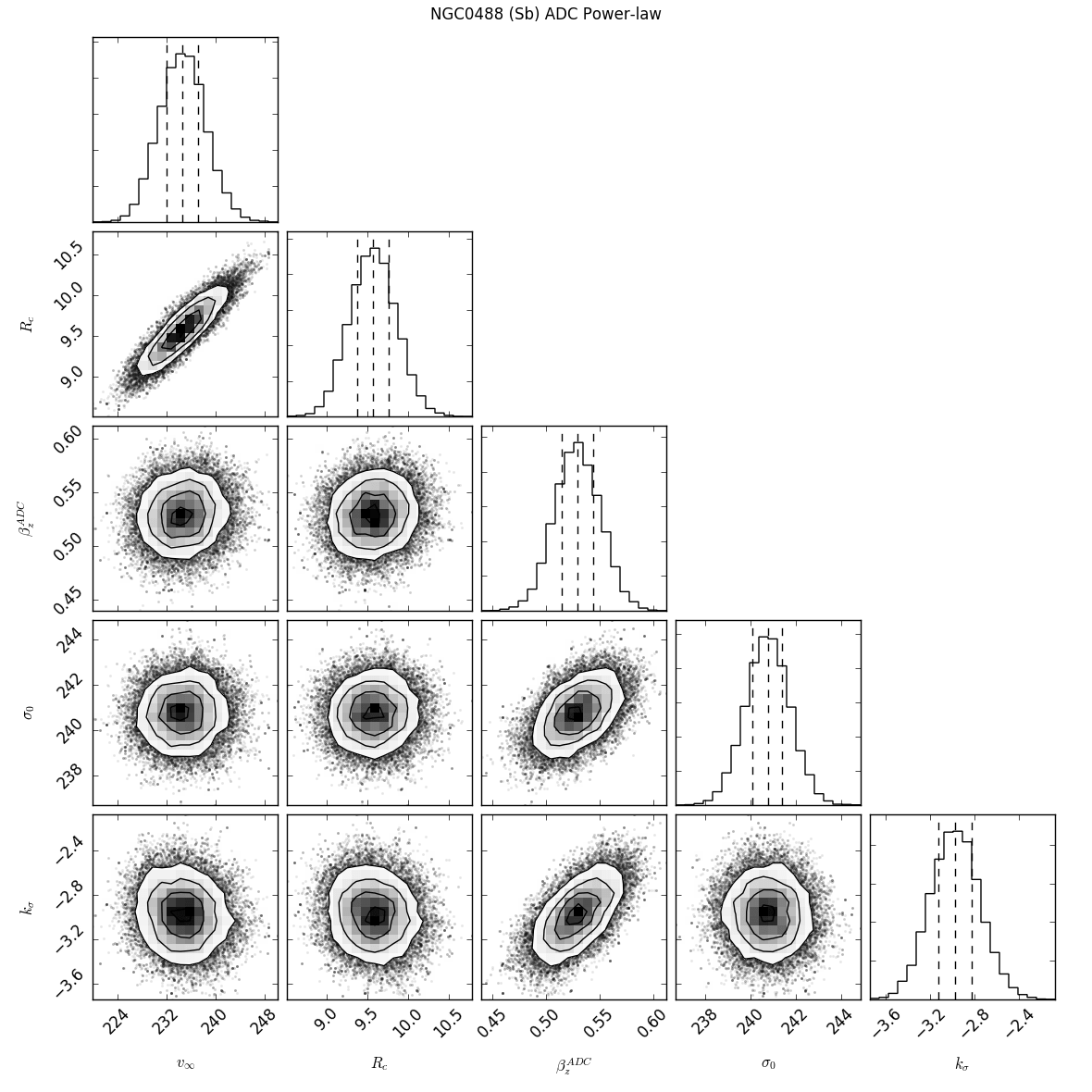
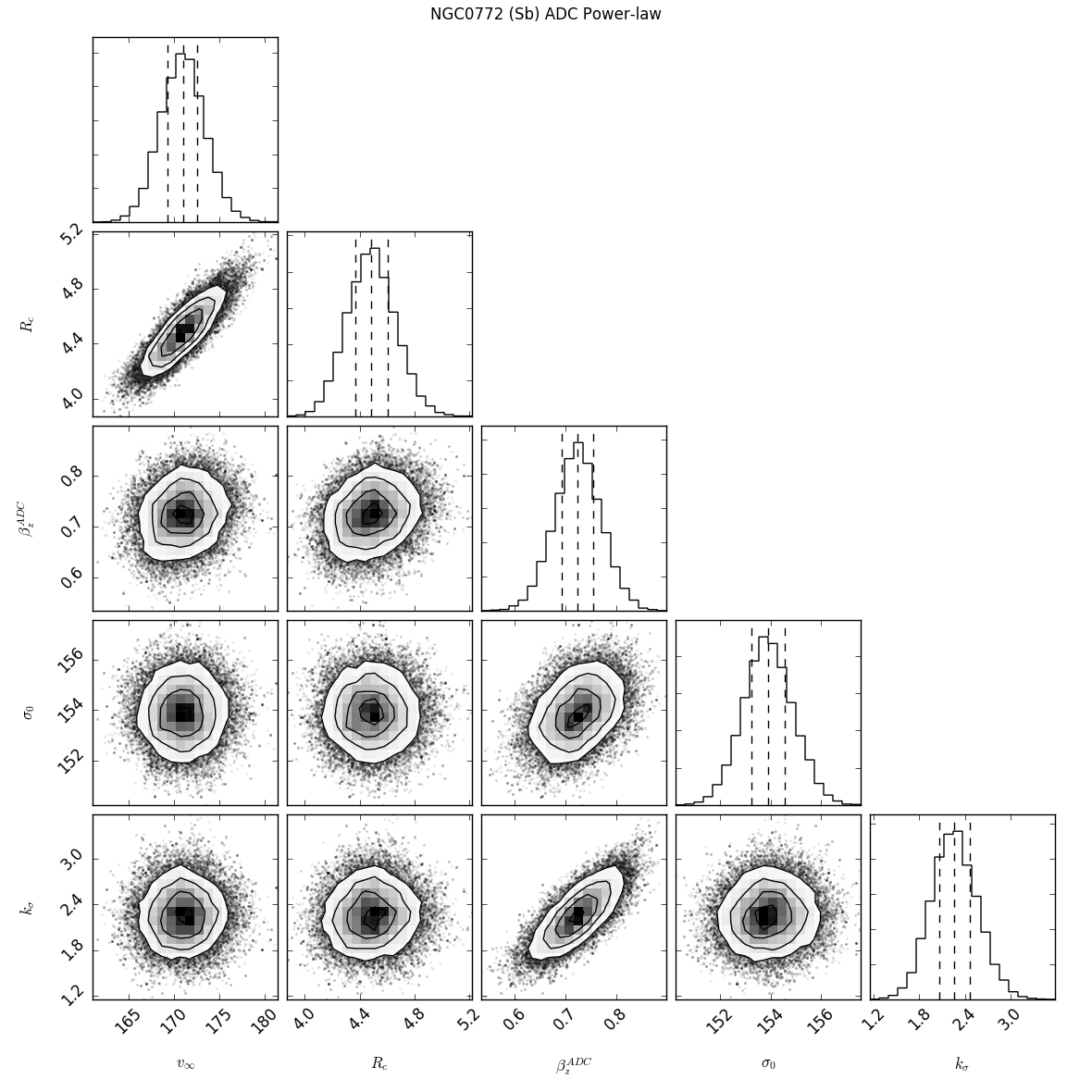
Figure 10: Corner plot shows the covariance between the model parameters of the 18 galaxies from ADC-MCMC method. Overplotted are the median value of the distributions related to the fitted parameters, together with their uncertainties at 25 and 75 percentiles.

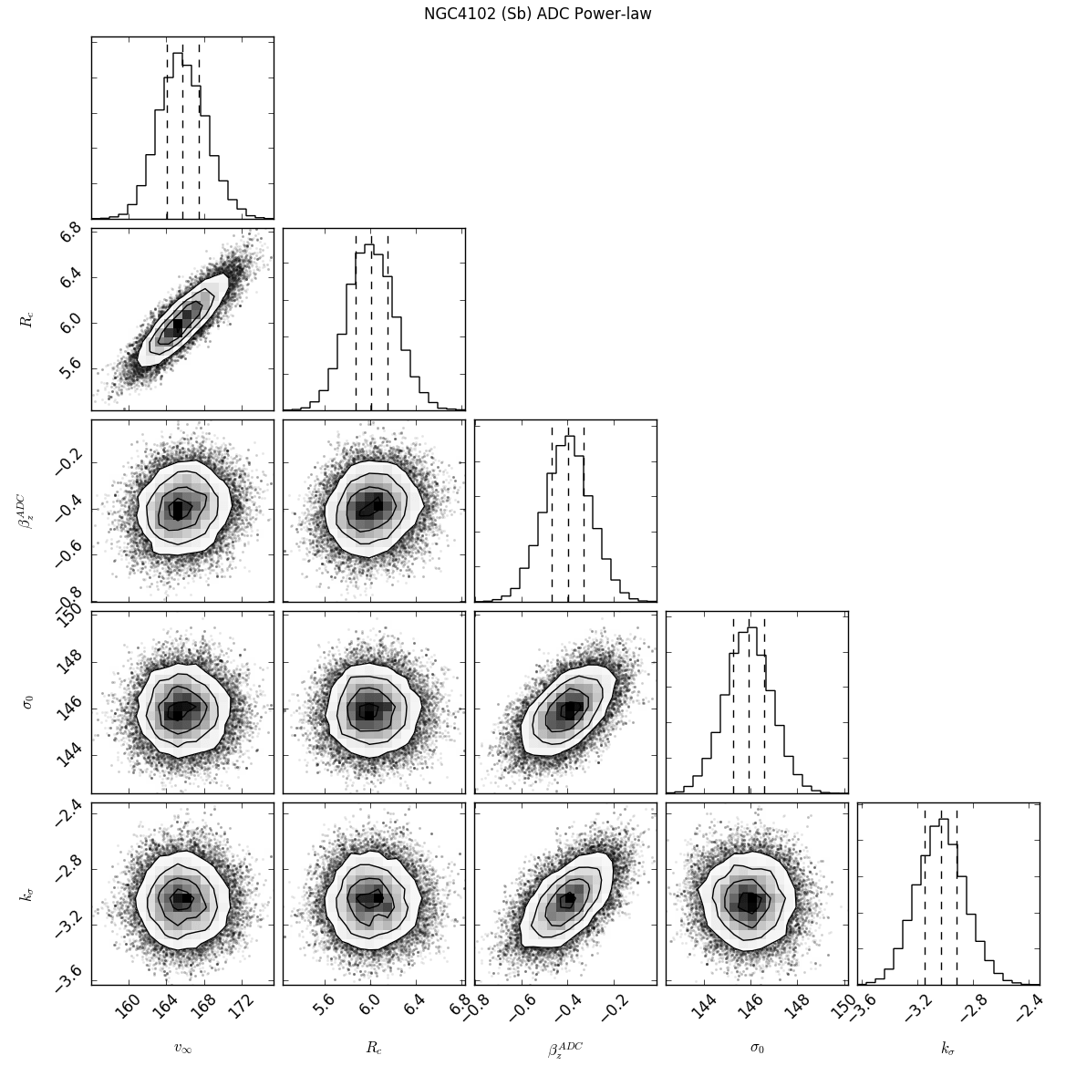
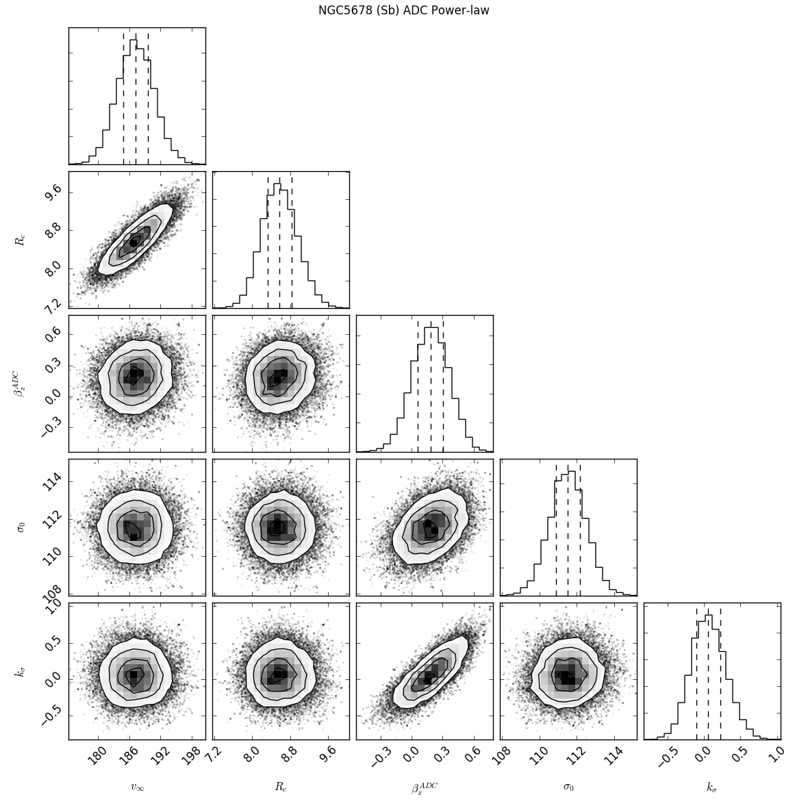
Figure 10: – continuation

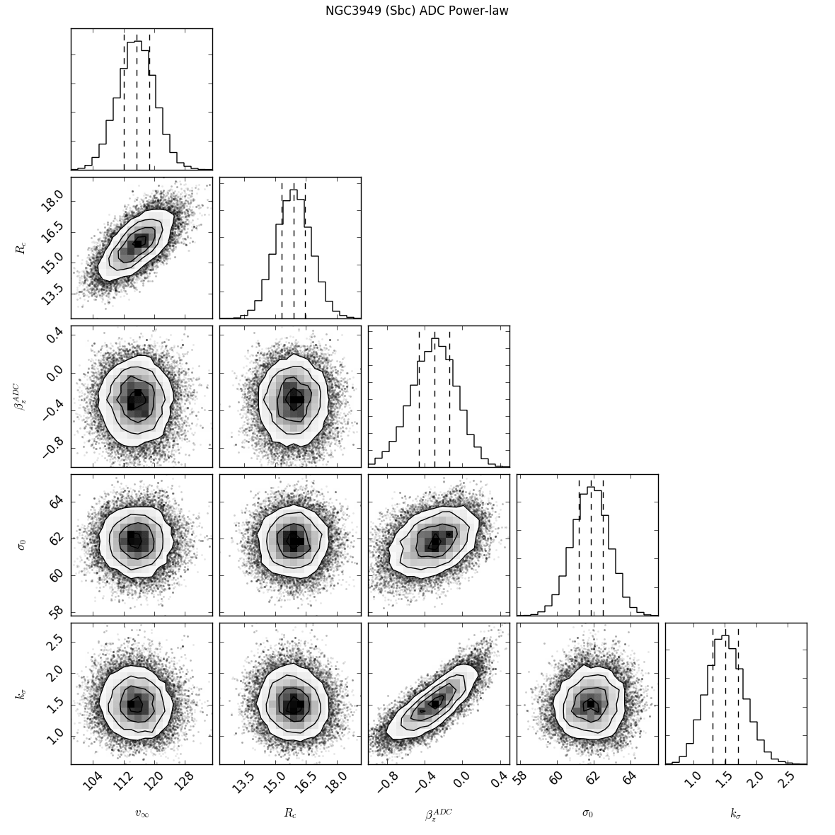
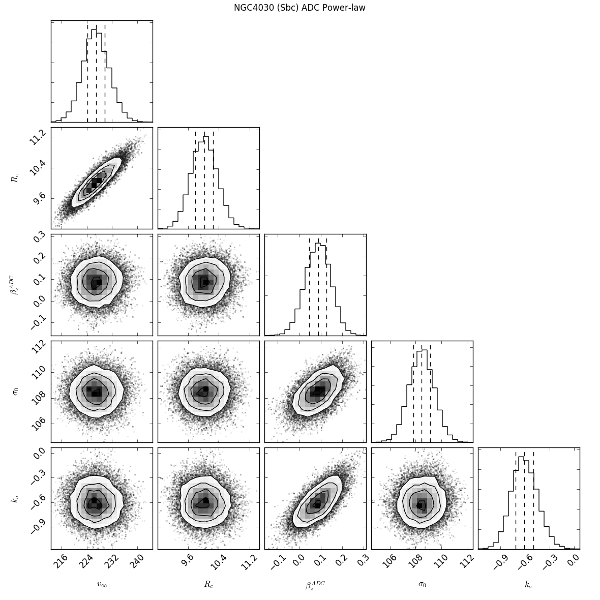
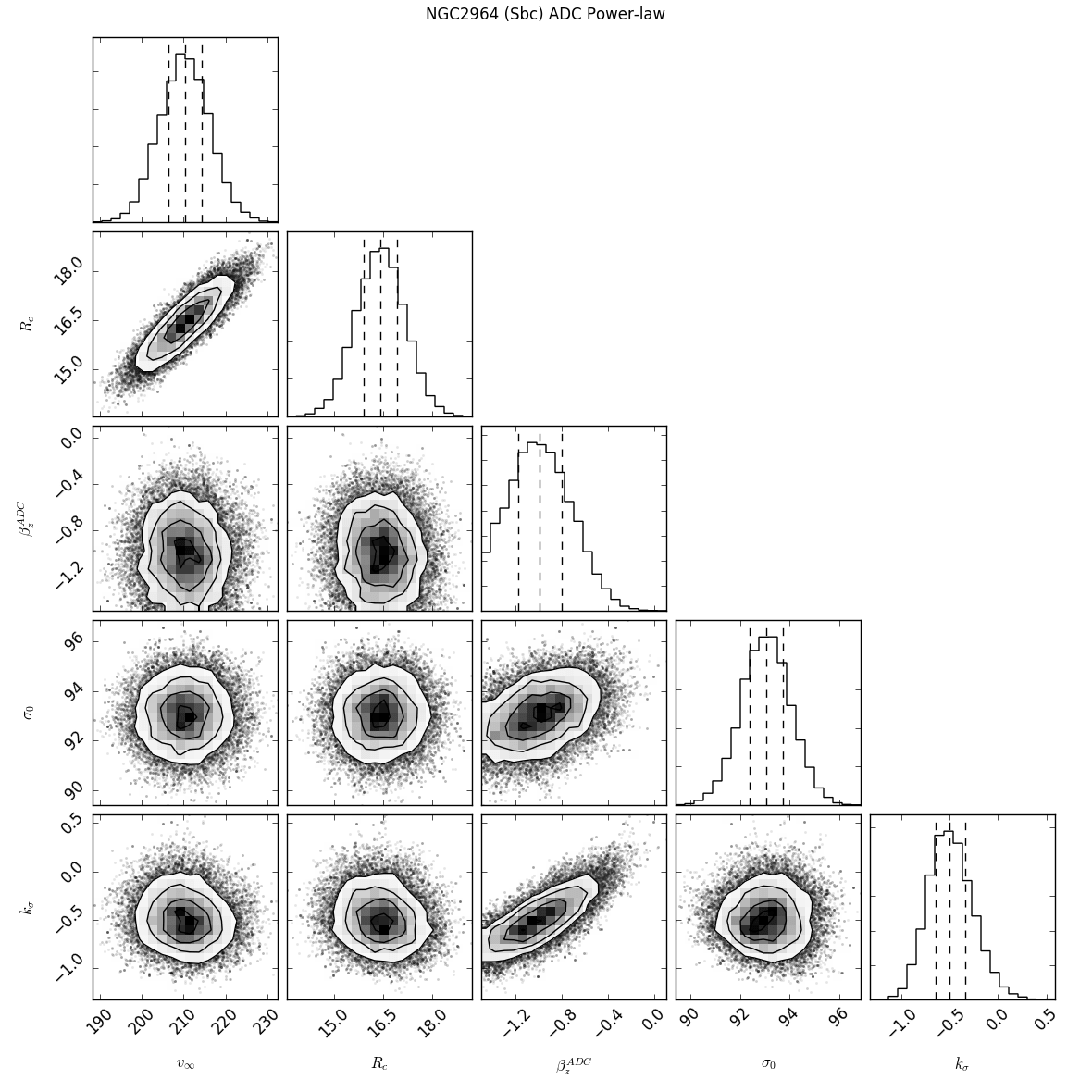
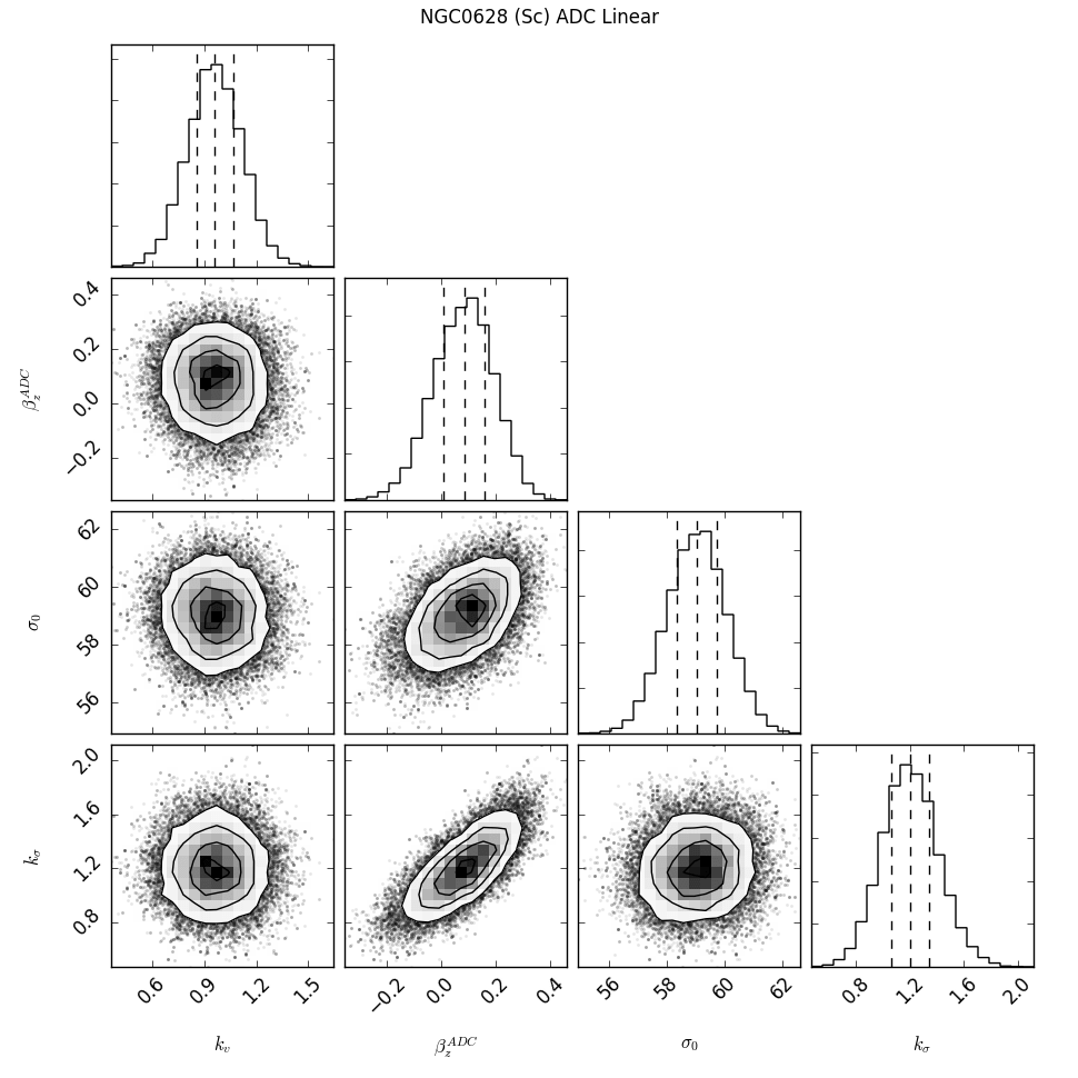
Figure 10: – continuation

Figure 10: – continuation

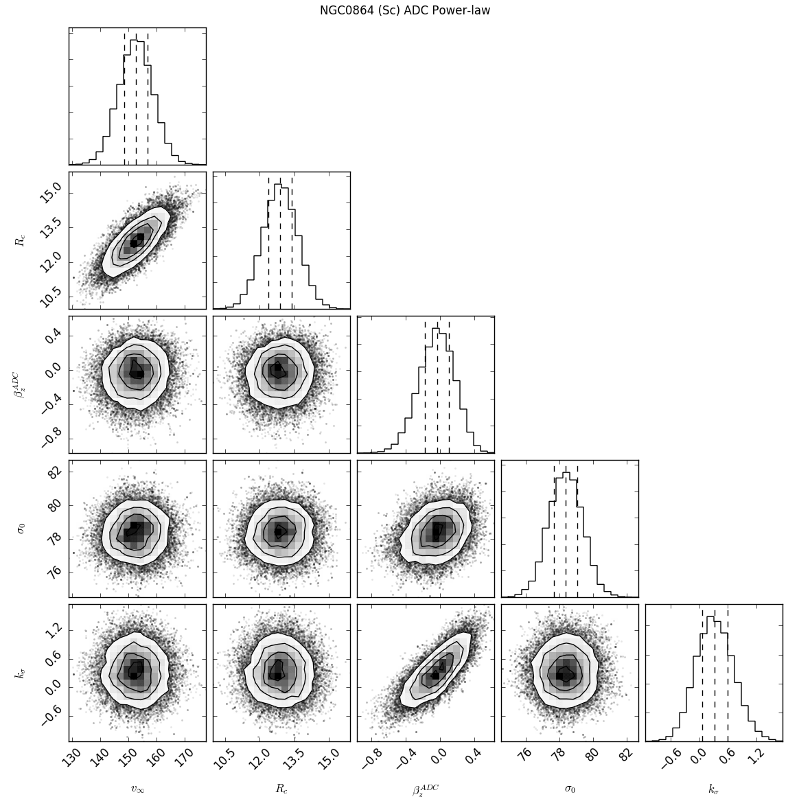
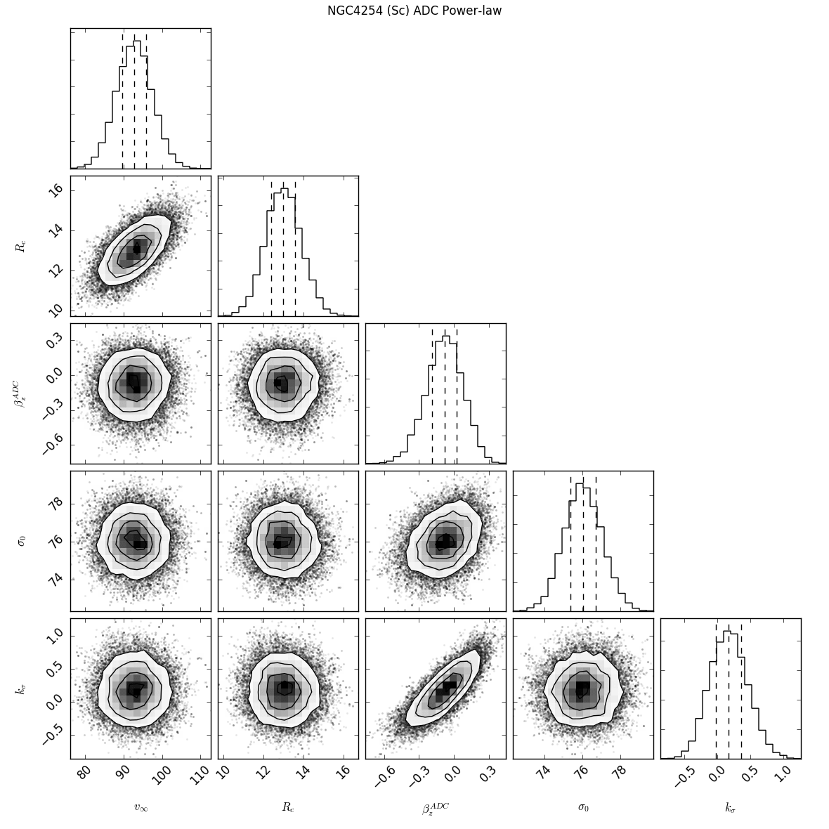
Figure 10: – continuation

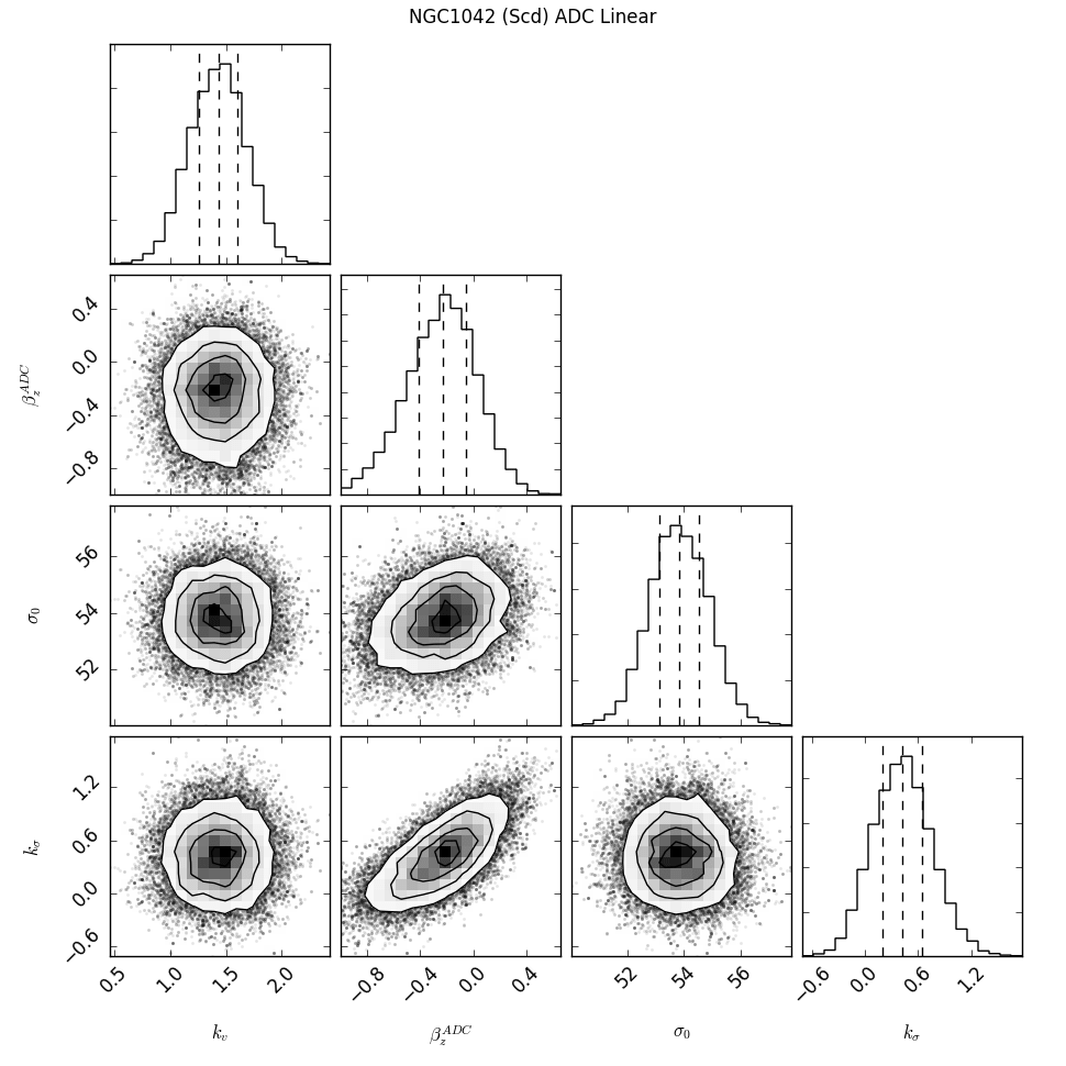
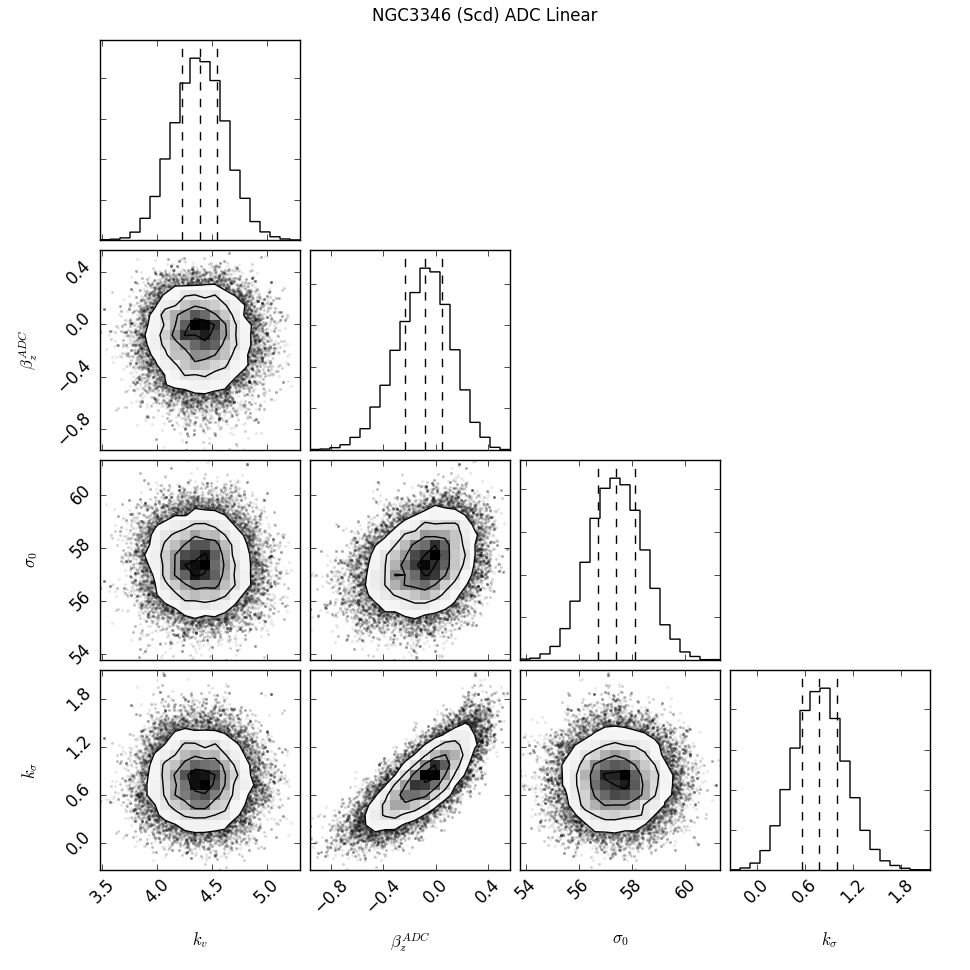
Figure 10: – continuation

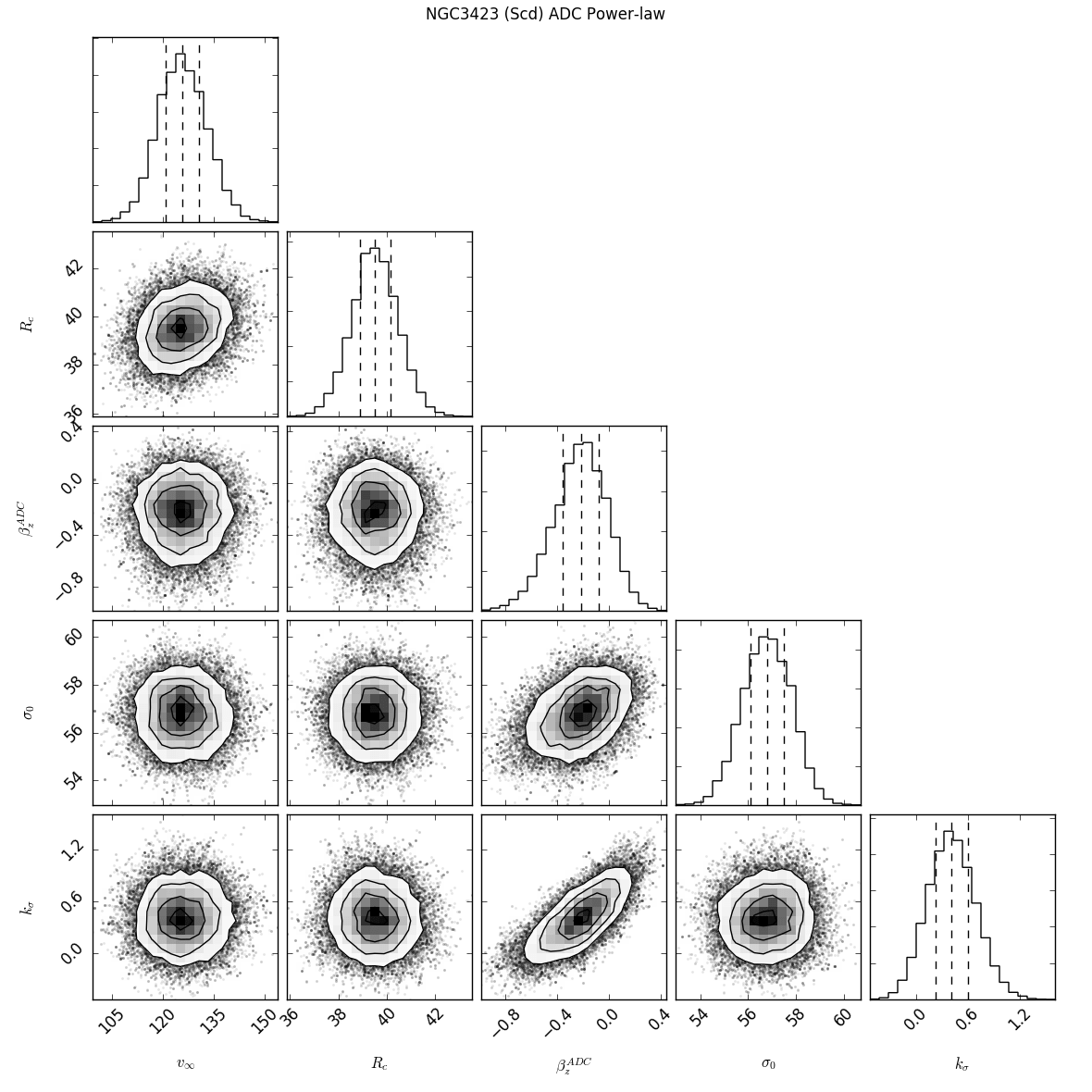
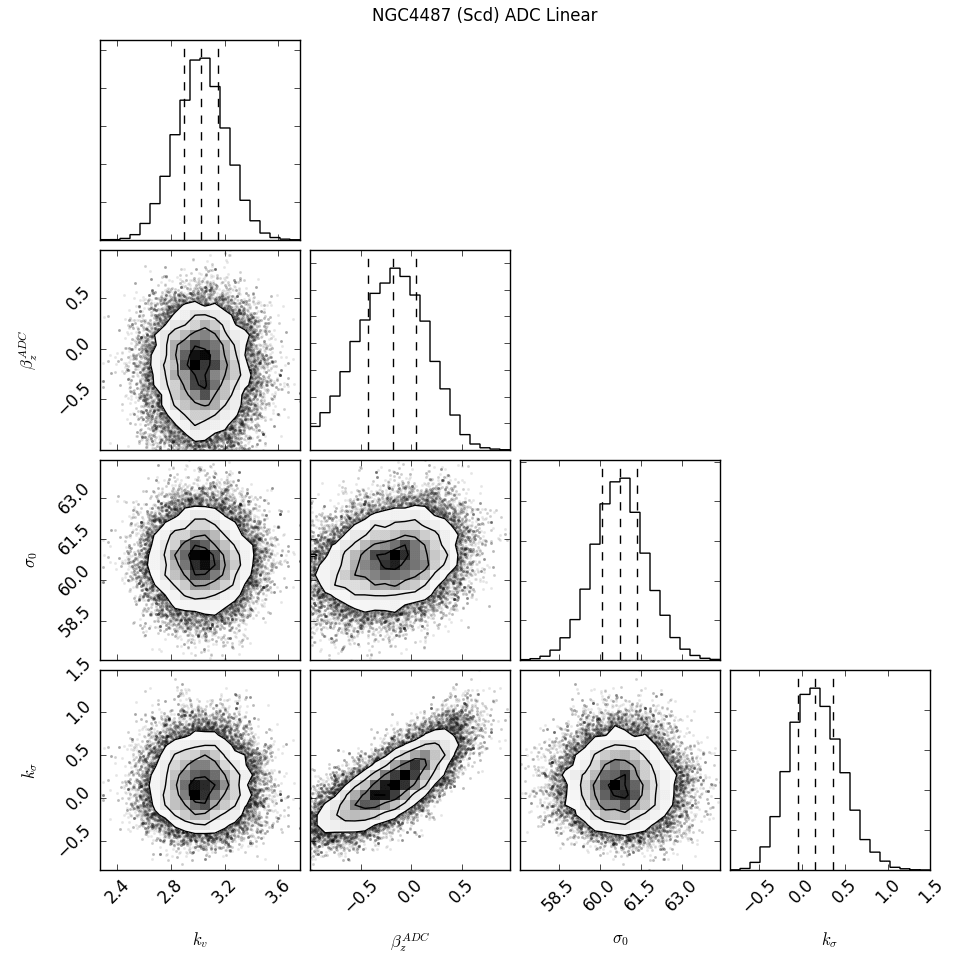
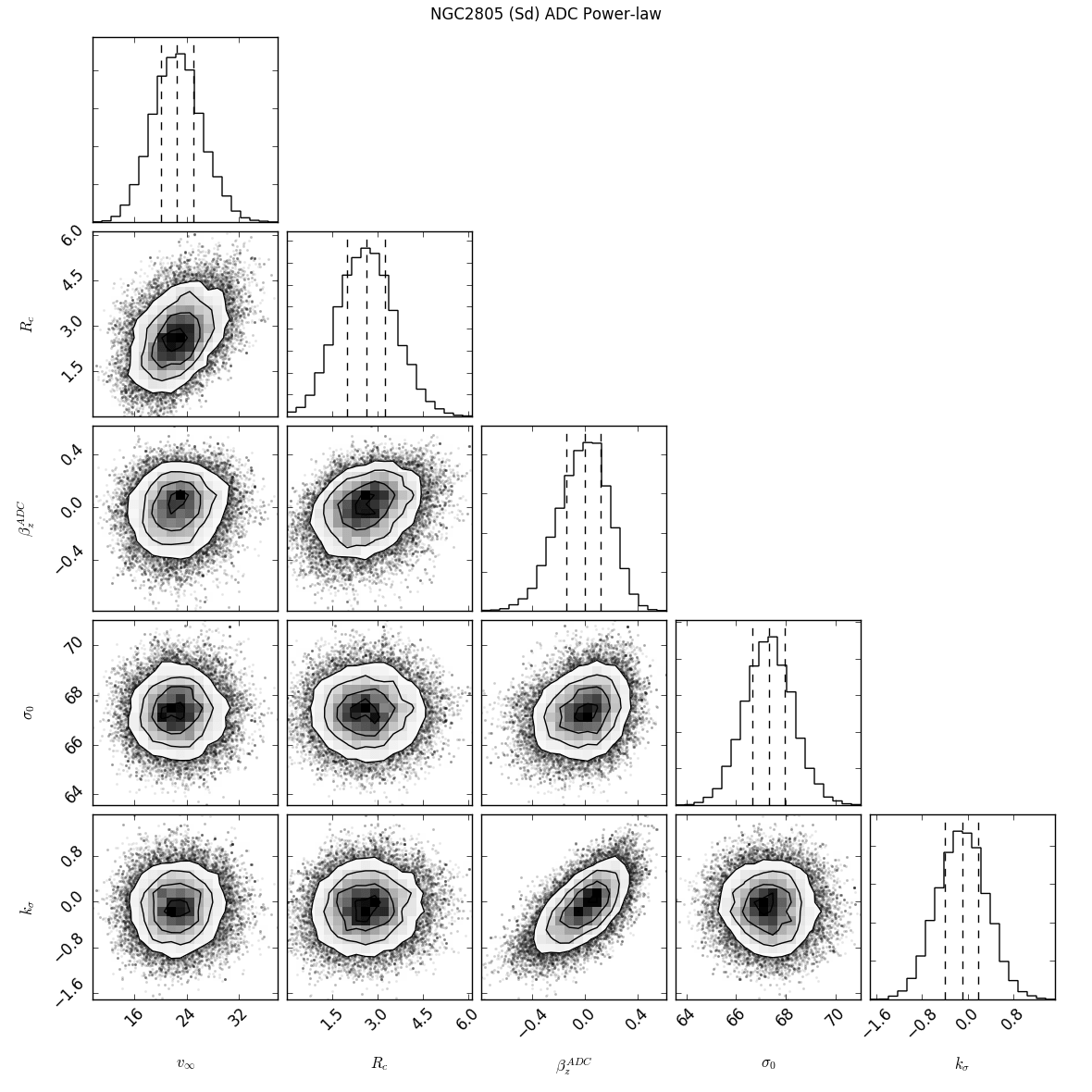
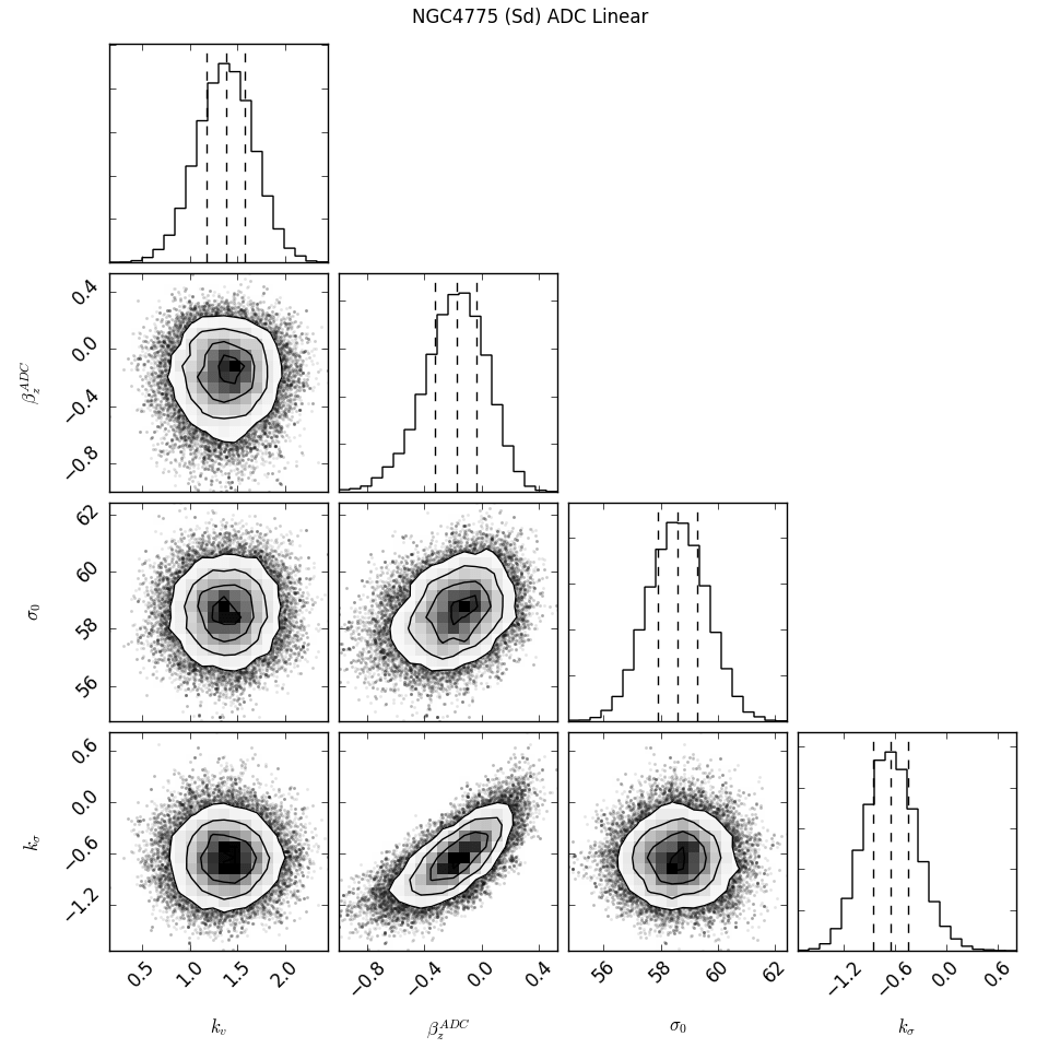
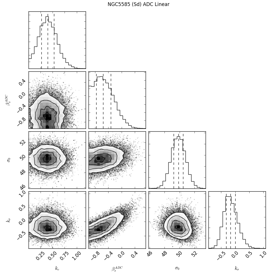
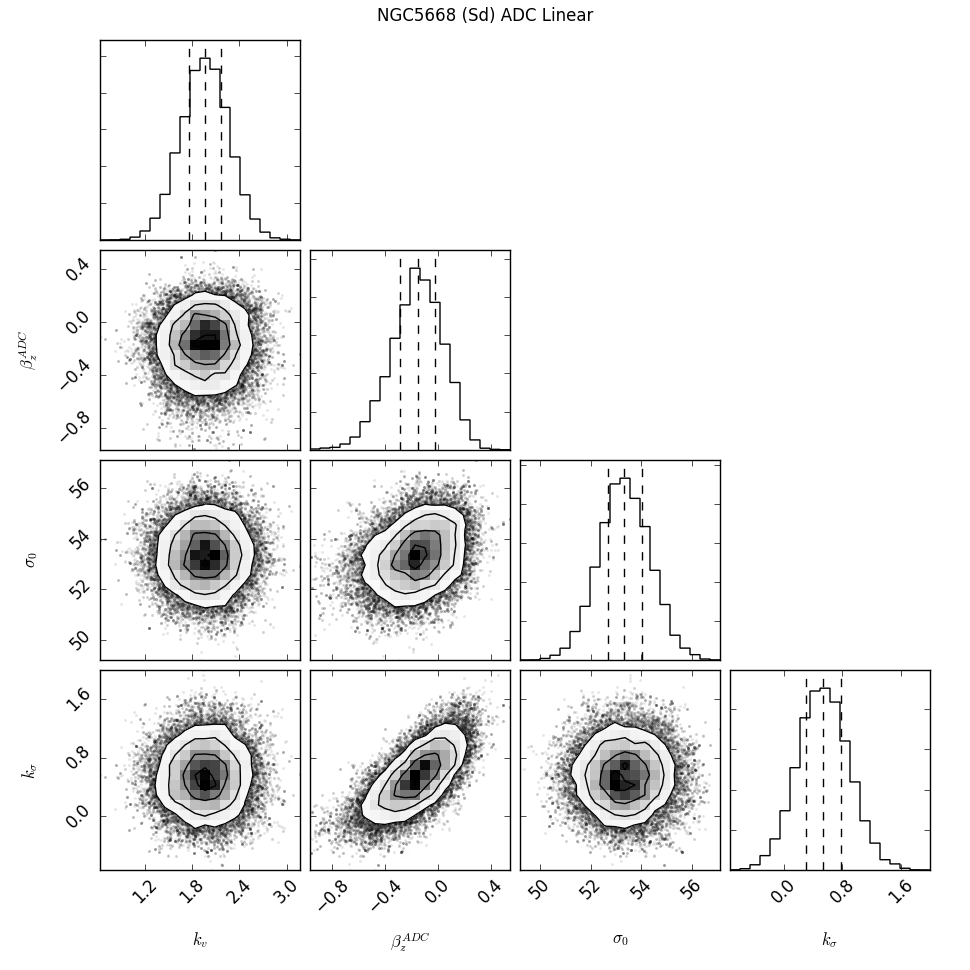
Figure 11: – continuation

Figure 11: – continuation

Figure 11: – continuation

References

- Aguerri, Beckman & Prieto (1998) Aguerri J. A. L., Beckman J. E., Prieto M., 1998, AJ, 116, 2136
- Bacon et al. (2001) Bacon R. et al., 2001, MNRAS, 326, 23
- Baes et al. (2003) Baes M. et al., 2003, MNRAS, 343, 1081
- Bedregal, Aragón-Salamanca & Merrifield (2006) Bedregal A. G., Aragón-Salamanca A., Merrifield M. R., 2006, MNRAS, 373, 1125
- Begeman (1987) Begeman K. G., 1987, PhD thesis, , Kapteyn Institute, (1987)
- Bershady et al. (2010) Bershady M. A., Verheijen M. A. W., Westfall K. B., Andersen D. R., Swaters R. A., Martinsson T., 2010, ApJ, 716, 234
- Binney & Merrifield (1998) Binney J., Merrifield M., 1998, Galactic Astronomy
- Binney & Tremaine (2008) Binney J., Tremaine S., 2008, Galactic Dynamics: Second Edition. Princeton University Press
- Blanc et al. (2013) Blanc G. A. et al., 2013, ApJ, 764, 117
- Böker et al. (2002) Böker T., Laine S., van der Marel R. P., Sarzi M., Rix H.-W., Ho L. C., Shields J. C., 2002, AJ, 123, 1389
- Bosma (1978) Bosma A., 1978, PhD thesis, PhD Thesis, Groningen Univ., (1978)
- Bottema (1993) Bottema R., 1993, A&A, 275, 16
- Buta & Zhang (2009) Buta R. J., Zhang X., 2009, ApJS, 182, 559
- Caldú-Primo et al. (2013) Caldú-Primo A., Schruba A., Walter F., Leroy A., Sandstrom K., de Blok W. J. G., Ianjamasimanana R., Mogotsi K. M., 2013, AJ, 146, 150
- Cappellari (2002) Cappellari M., 2002, MNRAS, 333, 400
- Cappellari (2008) Cappellari M., 2008, MNRAS, 390, 71
- Cappellari et al. (2006) Cappellari M. et al., 2006, MNRAS, 366, 1126
- Cappellari & Copin (2003) Cappellari M., Copin Y., 2003, MNRAS, 342, 345
- Cappellari & Emsellem (2004) Cappellari M., Emsellem E., 2004, PASP, 116, 138
- Cappellari et al. (2013) Cappellari M. et al., 2013, MNRAS, 432, 1862
- Cappellari et al. (2015) Cappellari M. et al., 2015, ApJ, 804, L21
- Carollo et al. (1997) Carollo C. M., Stiavelli M., de Zeeuw P. T., Mack J., 1997, AJ, 114, 2366
- Carollo, Stiavelli & Mack (1998) Carollo C. M., Stiavelli M., Mack J., 1998, AJ, 116, 68
- Carollo et al. (2002) Carollo C. M., Stiavelli M., Seigar M., de Zeeuw P. T., Dejonghe H., 2002, AJ, 123, 159
- Casertano (1983) Casertano S., 1983, MNRAS, 203, 735
- Colombo et al. (2014) Colombo D. et al., 2014, ApJ, 784, 4
- Comerón et al. (2011) Comerón S. et al., 2011, ApJ, 741, 28
- Conroy, Gunn & White (2009) Conroy C., Gunn J. E., White M., 2009, ApJ, 699, 486
- Dalcanton & Bernstein (2002) Dalcanton J. J., Bernstein R. A., 2002, AJ, 124, 1328
- Davis et al. (2013) Davis T. A. et al., 2013, MNRAS, 429, 534
- de Blok et al. (2008) de Blok W. J. G., Walter F., Brinks E., Trachternach C., Oh S.-H., Kennicutt, Jr. R. C., 2008, AJ, 136, 2648
- de Vaucouleurs (1991) de Vaucouleurs G., 1991, Science, 254, 1667
- Dehnen & Binney (1998) Dehnen W., Binney J. J., 1998, MNRAS, 298, 387
- Doménech-Moral et al. (2012) Doménech-Moral M., Martínez-Serrano F. J., Domínguez-Tenreiro R., Serna A., 2012, MNRAS, 421, 2510
- D’Onofrio et al. (1995) D’Onofrio M., Zaggia S. R., Longo G., Caon N., Capaccioli M., 1995, A&A, 296, 319
- Emsellem et al. (2004) Emsellem E. et al., 2004, MNRAS, 352, 721
- Emsellem, Monnet & Bacon (1994) Emsellem E., Monnet G., Bacon R., 1994, A&A, 285, 723
- Englmaier & Gerhard (1999) Englmaier P., Gerhard O., 1999, MNRAS, 304, 512
- Evans & de Zeeuw (1994) Evans N. W., de Zeeuw P. T., 1994, MNRAS, 271, 202
- Falcón-Barroso et al. (2006) Falcón-Barroso J. et al., 2006, MNRAS, 369, 529
- Falcón-Barroso et al. (2011) Falcón-Barroso J., Sánchez-Blázquez P., Vazdekis A., Ricciardelli E., Cardiel N., Cenarro A. J., Gorgas J., Peletier R. F., 2011, A&A, 532, A95
- Fathi et al. (2007) Fathi K., Beckman J. E., Zurita A., Relaño M., Knapen J. H., Daigle O., Hernandez O., Carignan C., 2007, A&A, 466, 905
- Foreman-Mackey et al. (2013) Foreman-Mackey D., Hogg D. W., Lang D., Goodman J., 2013, PASP, 125, 306
- Frogel (1988) Frogel J. A., 1988, ARA&A, 26, 51
- Fuchs et al. (2009) Fuchs B. et al., 2009, AJ, 137, 4149
- Ganda (2007) Ganda K., 2007, PhD thesis, University of Groningen
- Ganda et al. (2006) Ganda K., Falcón-Barroso J., Peletier R. F., Cappellari M., Emsellem E., McDermid R. M., de Zeeuw P. T., Carollo C. M., 2006, MNRAS, 367, 46
- Ganda et al. (2009) Ganda K., Peletier R. F., Balcells M., Falcón-Barroso J., 2009, MNRAS, 395, 1669
- Gerssen, Kuijken & Merrifield (1997) Gerssen J., Kuijken K., Merrifield M. R., 1997, MNRAS, 288, 618
- Gerssen, Kuijken & Merrifield (2000) Gerssen J., Kuijken K., Merrifield M. R., 2000, MNRAS, 317, 545
- Hubble (1926) Hubble E. P., 1926, ApJ, 64, 321
- Hunter (1977) Hunter C., 1977, AJ, 82, 271
- Ianjamasimanana et al. (2015) Ianjamasimanana R., de Blok W. J. G., Walter F., Heald G. H., Caldú-Primo A., Jarrett T. H., 2015, AJ, 150, 47
- Jeans (1915) Jeans J. H., 1915, MNRAS, 76, 70
- Kent (1986) Kent S. M., 1986, AJ, 91, 1301
- Koyama & Ostriker (2009) Koyama H., Ostriker E. C., 2009, ApJ, 693, 1346
- Krajnović et al. (2006) Krajnović D., Cappellari M., de Zeeuw P. T., Copin Y., 2006, MNRAS, 366, 787
- Kranz, Slyz & Rix (2003) Kranz T., Slyz A., Rix H.-W., 2003, ApJ, 586, 143
- Kregel & van der Kruit (2005) Kregel M., van der Kruit P. C., 2005, MNRAS, 358, 481
- Kregel, van der Kruit & de Grijs (2002) Kregel M., van der Kruit P. C., de Grijs R., 2002, MNRAS, 334, 646
- Kregel, van der Kruit & Freeman (2005) Kregel M., van der Kruit P. C., Freeman K. C., 2005, MNRAS, 358, 503
- Lablanche et al. (2012) Lablanche P.-Y. et al., 2012, MNRAS, 424, 1495
- Laine et al. (2002) Laine S., Shlosman I., Knapen J. H., Peletier R. F., 2002, ApJ, 567, 97
- Leroy et al. (2008) Leroy A. K., Walter F., Brinks E., Bigiel F., de Blok W. J. G., Madore B., Thornley M. D., 2008, AJ, 136, 2782
- Lilly (1989) Lilly S. J., 1989, ApJ, 340, 77
- Lynden-Bell (1962) Lynden-Bell D., 1962, MNRAS, 123, 447
- Maraston (2005) Maraston C., 2005, MNRAS, 362, 799
- Martinsson et al. (2013a) Martinsson T. P. K., Verheijen M. A. W., Westfall K. B., Bershady M. A., Schechtman-Rook A., Andersen D. R., Swaters R. A., 2013a, A&A, 557, A130
- Martinsson et al. (2013b) Martinsson T. P. K., Verheijen M. A. W., Westfall K. B., Bershady M. A., Schechtman-Rook A., Andersen D. R., Swaters R. A., 2013b, A&A, 557, A130
- Melbourne et al. (2012) Melbourne J. et al., 2012, ApJ, 748, 47
- Mignard (2000) Mignard F., 2000, A&A, 354, 522
- Monnet, Bacon & Emsellem (1992) Monnet G., Bacon R., Emsellem E., 1992, A&A, 253, 366
- Morganti et al. (2013) Morganti L., Gerhard O., Coccato L., Martinez-Valpuesta I., Arnaboldi M., 2013, MNRAS, 431, 3570
- Neistein et al. (1999) Neistein E., Maoz D., Rix H.-W., Tonry J. L., 1999, AJ, 117, 2666
- Noordermeer et al. (2007) Noordermeer E., van der Hulst J. M., Sancisi R., Swaters R. S., van Albada T. S., 2007, MNRAS, 376, 1513
- Rieke & Lebofsky (1985) Rieke G. H., Lebofsky M. J., 1985, ApJ, 288, 618
- Rix et al. (1997) Rix H.-W., de Zeeuw P. T., Cretton N., van der Marel R. P., Carollo C. M., 1997, ApJ, 488, 702
- Rix & Zaritsky (1995) Rix H.-W., Zaritsky D., 1995, ApJ, 447, 82
- Rodríguez & Padilla (2013) Rodríguez S., Padilla N. D., 2013, MNRAS, 434, 2153
- Rubin & Ford (1983) Rubin V. C., Ford, Jr. W. K., 1983, ApJ, 271, 556
- Ryś, Falcón-Barroso & van de Ven (2013) Ryś A., Falcón-Barroso J., van de Ven G., 2013, MNRAS, 428, 2980
- Sánchez-Blázquez et al. (2006) Sánchez-Blázquez P. et al., 2006, MNRAS, 371, 703
- Schwarzschild (1979) Schwarzschild M., 1979, ApJ, 232, 236
- Seth, Dalcanton & de Jong (2005) Seth A. C., Dalcanton J. J., de Jong R. S., 2005, AJ, 130, 1574
- Shapiro, Gerssen & van der Marel (2003) Shapiro K. L., Gerssen J., van der Marel R. P., 2003, AJ, 126, 2707
- Toloba et al. (2011) Toloba E., Boselli A., Cenarro A. J., Peletier R. F., Gorgas J., Gil de Paz A., Muñoz-Mateos J. C., 2011, A&A, 526, A114
- Tully & Pierce (2000) Tully R. B., Pierce M. J., 2000, ApJ, 533, 744
- van Albada et al. (1985) van Albada T. S., Bahcall J. N., Begeman K., Sancisi R., 1985, ApJ, 295, 305
- van de Ven et al. (2010) van de Ven G., Falcón-Barroso J., McDermid R. M., Cappellari M., Miller B. W., de Zeeuw P. T., 2010, ApJ, 719, 1481
- van de Ven et al. (2006) van de Ven G., van den Bosch R. C. E., Verolme E. K., de Zeeuw P. T., 2006, A&A, 445, 513
- van den Bosch et al. (2006) van den Bosch R., de Zeeuw T., Gebhardt K., Noyola E., van de Ven G., 2006, ApJ, 641, 852
- van den Bosch & de Zeeuw (2010) van den Bosch R. C. E., de Zeeuw P. T., 2010, MNRAS, 401, 1770
- van den Bosch et al. (2008) van den Bosch R. C. E., van de Ven G., Verolme E. K., Cappellari M., de Zeeuw P. T., 2008, MNRAS, 385, 647
- Vandervoort (1975) Vandervoort P. O., 1975, ApJ, 195, 333
- Vorobyov & Theis (2008) Vorobyov E. I., Theis C., 2008, MNRAS, 383, 817
- Wada & Koda (2004) Wada K., Koda J., 2004, MNRAS, 349, 270
- Weijmans et al. (2008) Weijmans A.-M., Krajnović D., van de Ven G., Oosterloo T. A., Morganti R., de Zeeuw P. T., 2008, MNRAS, 383, 1343
- Weiner, Sellwood & Williams (2001) Weiner B. J., Sellwood J. A., Williams T. B., 2001, ApJ, 546, 931
- Williams, Bureau & Cappellari (2010) Williams M. J., Bureau M., Cappellari M., 2010, MNRAS, 409, 1330
- Yoachim & Dalcanton (2006) Yoachim P., Dalcanton J. J., 2006, AJ, 131, 226
- Zibetti, Charlot & Rix (2009) Zibetti S., Charlot S., Rix H.-W., 2009, MNRAS, 400, 1181
- Zibetti et al. (2013) Zibetti S., Gallazzi A., Charlot S., Pierini D., Pasquali A., 2013, MNRAS, 428, 1479