Kinetics of Ferromagnetic Ordering in 3D Ising Model: Do we understand the case of zero temperature quench?

Abstract

We study phase ordering dynamics in the three-dimensional nearest-neighbor Ising model, following rapid quenches from infinite to zero temperature. Results on various aspects, viz., domain growth, persistence, aging and pattern, have been obtained via the Glauber Monte Carlo simulations of the model on simple cubic lattice. These are analyzed via state-of-the-art methods, including the finite-size scaling, and compared with those for quenches to a temperature above the roughening transition. Each of these properties exhibit remarkably different behavior at the above mentioned final temperatures. Such a temperature dependence is absent in the two-dimensional case for which there is no roughening transition.

I Introduction

When a paramagnetic system is quenched inside the ferromagnetic region, by a change of the temperature from $T_{i}$ ($>T_{c}$) to $T_{f}$ ($<T_{c}$), $T_{c}$ being the critical temperature, it becomes unstable to fluctuations onuki ; bray_phase ; puri . Such an out-of-equilibrium system moves towards the new equilibrium via the formation and growth of domains onuki ; bray_phase ; puri . These domains are rich in atomic magnets aligned in the same direction and grow with time ($t$) via the curvature driven motion of the interfaces bray_phase ; Allen_cahn ; puri . The interface velocity scales with $\ell$, the average domain size, as bray_phase ; Allen_cahn

$$\frac{d\ell}{dt}\sim\frac{1}{\ell}.$$ (1)

This provides a power-law growth bray_phase ; Allen_cahn

$$\ell\sim t^{\alpha},$$ (2)

with $\alpha=1/2$. Depending upon the order-parameter symmetry and system dimensionality ($d$), there may exist corrections to this growth law bray_phase .

Apart from the above mentioned change in the characteristic length scale, the domain patterns at different times, during the growth process, are statistically self-similar bray_phase ; puri . This is reflected in the scaling property bray_phase ,

$$C(r,t)\equiv\tilde{C}(r/\ell),$$ (3)

of the two-point equal-time correlation function $C$, where $r$ ($=|{\vec{r}_{1}-\vec{r}_{2}}|$) is the scalar distance between two space points and $\tilde{C}$ is a master function, independent of time. A more general correlation function involves two space points and two times, and is defined as puri

$$C(\vec{r}_{1},t_{w};\vec{r}_{2},t)=~{}~{}~{}~{}~{}~{}~{}~{}~{}~{}~{}~{}~{}~{}~{}~{}~{}$$

$$\langle\psi(\vec{r}_{1},t_{w})\psi(\vec{r}_{2},t)\rangle-\langle\psi(\vec{r}_{1},t_{w})\rangle\langle\psi(\vec{r}_{2},t)\rangle,$$ (4)

where $\psi$ is a space and time dependent order parameter. The total value of the order parameter, obtained by integrating $\psi$ over the whole system, is not time invariant for a ferromagnetic ordering bray_phase . Thus, the coarseing in this case belongs to the category of “nonconserved” order parameter dynamics bray_phase . For $\vec{r}_{1}=\vec{r}_{2}$, the definition in Eq. (I) corresponds to the two-time autocorrelation function, frequently used for the study of aging property puri ; fisher_huse ; cor_lippi of an out-of-equilibrium system, $t_{w}(\leq t)$ being referred to as the waiting time or the age of the system. For the two point equal-time case, on the other hand, $t_{w}=t$. The autocorrelation will henceforth be denoted as $C_{\rm ag}(t,t_{w})$. This quantity usually scales as puri ; fisher_huse ; cor_lippi ; liu ; satya_huse ; yrd ; henkel

$$C_{\rm ag}(t,t_{w})=\tilde{C}_{\rm ag}(\ell/\ell_{w}),$$ (5)

where $\tilde{C}_{\rm ag}$ is another master function, independent of $t_{w}$, and $\ell_{w}$ is the value of $\ell$ at $t_{w}$. Another interesting quantity, in the context of phase ordering dynamics, is the persistence probability $P$ bray_per ; satya_sire ; satya_bray ; derrida ; stauffer ; manoj_1 ; godreche ; stauffer_jpa . This is defined as the fraction of unaffected atomic magnets (or spins) and decays in a power-law fashion with time as bray_per

$$P\sim t^{-\theta}.$$ (6)

In the area of nonequilibrium statistical physics, there has been immense interest in estimating the exponents $\alpha$ and $\theta$, as well as in obtaining the functional forms of $\tilde{C}$ and $\tilde{C}_{\rm ag}$, via analytical theories and computer simulations bray_phase ; puri ; bray_per .

In this work, we study all these properties for the nonconserved coarsening dynamics in the Ising model d_landau ,

$$H=-J\sum_{<ij>}S_{i}S_{j},~{}J>0,~{}S_{i}=\pm 1,$$ (7)

via Monte Carlo (MC) simulations d_landau . We focus on $d=3$ and study ordering at $T_{f}=0$, for rapid quenches from $T_{i}=\infty$. This dimension, particularly for $T_{f}=0$, received less attention compared to the $d=2$ case. In $d=2$, the MC results for $C(r,t)$ are found to be in nice agreement with the Ohta-Jasnow-Kawasaki (OJK) function bray_phase ; ojk ; puri ($D$ being a diffusion constant)

$$C(r,t)=\frac{2}{\pi}\sin^{-1}\bigg{[}\exp\bigg{(}-\frac{r^{2}}{8Dt}\bigg{)}\bigg{]}.$$ (8)

This expression also implies $\alpha=1/2$, validity of which has been separately checked bray_phase ; puri . For the latter dimension, in the long time limit, the autocorrelation is understood to scale with $x$ ($=\ell/\ell_{w}$) as fisher_huse ; liu ; henkel ; jia_suman

$$C_{\rm ag}(t,t_{w})\sim x^{-\lambda},$$ (9)

with $\lambda$ following a lower bound,

$$\lambda\geqslant\frac{d}{2},$$ (10)

predicted by Fisher and Huse (FH) fisher_huse . In this case, also the persistence exponent $\theta$ has been estimated stauffer ; manoj_1 ; blanchard ; saikat for quenches to $T_{f}=0$. Furthermore, a few of these aspects, viz., the equal-time correlation function and domain growth, are understood to be independent of the value of $T_{f}$.

Our interest in the zero temperature quench for $d=3$ was drawn by a controversy amar_family ; holzer ; cueille_jpa ; corberi , following reports from computer simulations that observed $\alpha=1/3$ for this particular case, while the theoretical prediction is independent of $d$ and $T_{f}$. While addressing this issue, via simulations with large system sizes over long period, we made further interesting observations in other quantities. In this paper, we present these results on pattern, growth, aging and persistence. While our studies for pattern and aging are new, the results for growth and persistence are presented in forms different from a previous work saikat_pre , to bring completeness to the discussion. It appears, previous conclusion on the value of $\alpha$ was led by the presence of an exceptionally long transient period, which was later hinted in Ref. corberi . In the “true” long time limit, the growth exponent is indeed $1/2$. Such a trend we observe in the decay of the persistence probability as well. On the other hand, the pattern and aging properties do not exhibit any crossover. These results are very much different from those obtained for quenches to a temperature above the roughening temperature. Such temperature dependence does not exist in the $d=2$ case. Wherever necessary we presented results from the latter dimension as well.

The rest of the paper is organized as follows. In section II we describe the methods. Results are presented in section III. Finally, we conclude the paper in section IV by presenting a summary.

II Methods

All our results were obtained via MC simulations of the Ising model using Glauber kinetics d_landau ; glauber , where, in each trial move the sign of a randomly chosen spin was changed. For $T_{f}=0$, the move was accepted if it brought a negative change in the energy. On the other hand, for $T_{f}>0$, whenever a trial move brought a higher energy contribution, the acceptance was decided by comparing the corresponding Boltzmann factor with a random number (drawn from an uniform distribution), a standard practice followed in the Metropolis algorithm d_landau .

In $d=2$ we have used square lattice and for $d=3$ the results are from simple cubic lattice. All simulations were performed in periodic boxes of volume $V=L^{d}$, $L$ being the linear dimension of a box, in units of the lattice constant. For this model, the $d$-dependent critical temperatures d_landau are $T_{c}\simeq 2.269J/k_{B}$ ($d=2$) and $T_{c}\simeq 4.51J/k_{B}$ ($d=3$), $k_{B}$ being the Boltzmann constant. Time in our simulations was measured in units of MC step (MCS), each MCS consisting of $L^{d}$ trial moves d_landau . Unless otherwise mentioned, all results are presented after averaging over at least $10$ independent initial configurations, with $L=512$. For the rest of the paper we set $k_{B}$, tha lattice constant and the interaction strength ($J$) to unity.

The average domain size was calculated in two different ways: (i) from the first moment of the domain size distribution $P_{d}(\ell_{d},t)$ as suman

$$\ell=\int{\ell_{d}P_{d}(\ell_{d},t)d\ell_{d}},$$ (11)

$\ell_{d}$ being the distance between two successive interfaces along any direction, and (ii) using the scaling property of the correlation function as bray_phase

$$C(\ell,t)=0.1.$$ (12)

Unless otherwise mentioned, presented results are from Eq. (11). For this purpose, we have eliminated the noise in the configurations at nonzero temperatures, by applying a majority spin rule suman . Note that the order-parameter $\psi$ here is equivalent to the Ising spin variable $S_{i}$. Thus, further discussions on the calculation of the other quantities are not needed.

III Results

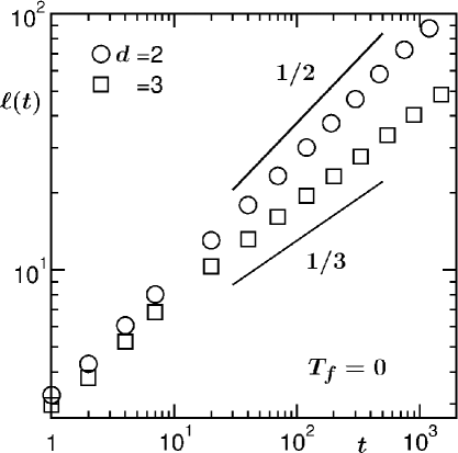
Figure 1: Log-log plots of the average domain length, $\ell(t)$, vs time, for $T_{f}=0$. Results from both $d=2$ and $3$ are presented. In both the cases linear dimension of the system is $L=200$. The solid lines correspond to two different power-law growths, exponents being mentioned in the figure.

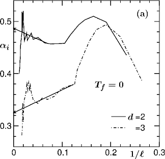
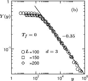
Figure 2: (a) Plots of the instantaneous exponent, $\alpha_{i}$, vs $1/\ell$, obtained from the data in Fig. 1. (b) Finite-size scaling exercise for the $d=3$ results for $\ell(t)$. Here we have shown the scaling function $Y$ with the variation of the dimensionless quantity $y$. $Y$ was obtained from the best collapse of data from three different system sizes (mentioned in the figure). The solid line corresponds to a power law decay with exponent $0.35$. All results are from $T_{f}=0$.

We start by showing the plots of $\ell$ vs $t$, for $d=2$ and $3$, at $T_{f}=0$, on a log-log scale, in Fig. 1. The system size considered here is comparable to the early studies amar_family ; holzer in $d=3$. The data for $d=2$ is clearly consistent with the exponent $\alpha=1/2$, for the whole time range bray_phase ; puri . On the other hand, after $t=10$ the $d=3$ data appear parallel to $\alpha=1/3$. For accurate estimation of the exponent for a power-law behavior it is useful to calculate the instantaneous exponent huse_1986

$$\alpha_{i}=\frac{d\ln\ell}{d\ln t},$$ (13)

as well as perform finite size scaling (FSS) analysis d_landau ; m_fisher . In Fig. 2(a) we plot $\alpha_{i}$ as a function of $1/\ell$. Clearly, for $d=3$, the convergence of the data set, in the limit $\ell=\infty$, is consistent with $\alpha=1/3$, while the $d=2$ data converge to $\alpha=1/2$. Since the data for large $\ell$ in this figure are noisy, to understand the stability of the $d=3$ exponent over long period, we perform the FSS analysis (see Fig. 2(b)). We do not perform this exercise for $d=2$, since, in this case we have already seen that the data are consistent with the theoretical expectation, as established previously bray_phase ; puri . In fact, from here on, unless otherwise mentioned, all results are from $d=3$ and $T_{f}=0$.

In analogy with the critical phenomena m_fisher , a finite-size scaling method in the domain growth problems can be constructed as suman ; heermann_binder ; das_epl

$$\ell(t)=LY(y),$$ (14)

where the finite-size scaling function $Y$ is independent of the system size but depends upon $y$ $(=L^{1/\alpha}/t)$, a dimensionless scaling variable. In the long time limit $(y\rightarrow 0)$, when $\ell\simeq L$, $Y$ should be a constant. At early time $(y>>0)$, on the other hand, the behavior of $Y$ should be such that Eq. (2) is recovered (since the finite-size effects in this limit are non-existent). Thus

$$Y(y>>0)\sim y^{-\alpha}.$$ (15)

In the FSS analysis, $\alpha$ is treated as an adjustable parameter. For appropriate choice of $\alpha$, in addition to observing the behavior in Eq. (15), data from all different values of $L$ should collapse onto a single master curve. In Fig. 2(b) we have used $\alpha=0.35$. The quality of collapse and the consistency of the power-law decay of the scaling function with the above quoted exponent, over several decades in $y$, confirm the stability of the value. Thus, it was not inappropriate for the previous studies amar_family ; holzer to conclude that the value of $\alpha$ is $1/3$. Nevertheless, given the increase of computational resources over last two decades, it is instructive to simulate larger systems over longer periods corberi , to check if a crossover to the theoretically expected exponent occurs at very late time.

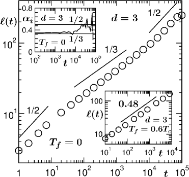
Figure 3: Log-log plot of $\ell(t)$ vs $t$, for $d=3$ and $T_{f}=0$, with $L=512$. The rest of the results are presented for this particular system size. The solid lines indicate different power-law growths, the exponents being mentioned. The upper inset shows instantaneous exponent $\alpha_{i}$ as a function of $t$, the $x$-axis being in log scale, for the data presented in the main frame. The horizontal solid lines there correspond to $\alpha=1/3$ and $1/2$. The lower inset is same as the main frame but for $T_{f}=0.6T_{c}$. The continuous line there corresponds to a power-law growth with exponent $0.48$.

In Fig. 3 we present the $\ell$ vs $t$ data, on a log-log scale, from a much larger system size saikat_pre than the ones considered in Figs. 1 and 2. Interestingly, three different regimes are clearly visible. A very early time regime shows consistency with $\alpha=1/2$. This is followed by an exponent $1/3$, that stays for about three decades in time. Finally, the expected $\alpha=1/2$ behavior is visible, for nearly a decade, before the finite size effects appear. In this case, an appropriate FSS analysis, to confirm the later time exponent, requires even bigger systems with runs over much longer times, which, given the resources available to us, was not possible. Thus, for an accurate quantification of the asymptotic value of $\alpha$, we restrict ourselves to the analysis via the instantaneous exponent huse_1986 . In the upper inset of Fig. 3, we have plotted $\alpha_{i}$ as a function of $t$. The qunatity shows a nice late time oscillation around the value $1/2$. This is at variance with the data at high temperature. See the $\ell$ vs $t$ data, on a log-log scale, from $T_{f}=0.6T_{c}$, in the lower inset of Fig. 3. Here we observe $\alpha=1/2$ for the whole time range. For this data set as well we avoid presenting results from further analyses.

For $T_{f}=0$, the crossover that occurs in the time dependence of $\ell$, may be present in other properties as well saikat_pre . These we check next. For the persistence probability, the value of $\theta$ was previously estimated manoj_1 , also from smaller system sizes, to be $\simeq 0.17$.

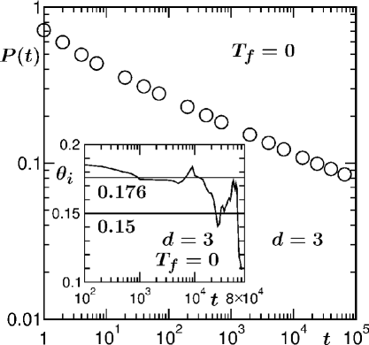
Figure 4: Log-log plot of the persistence probability, $P(t)$, as a function of $t$, for $d=3$ and $L=512$. The inset shows corresponding instantaneous exponent, $\theta_{i}$, vs $t$, $x$-axis being in a log scale. The horizontal solid lines there correspond to the ordinate values $0.176$ and $0.15$. The figure has resemblance with Fig. 7(b) of Physical Review E 93, 032139 (2016). These results are from $T_{f}=0$.

In Fig. 4 we show a log-log plot of $P$ vs $t$ and the corresponding instantaneous exponent $\theta_{i}$ (see the inset), calculated as huse_1986

$$\theta_{i}=-\frac{d\ln P}{d\ln t},$$ (16)

vs $t$, for the same (large) system as in Fig. 3. The early time data is consistent with the previous estimate. At late time there is a crossover saikat_pre to a smaller value $\simeq 0.15$, the crossover time being the same as that for the average domain size. Here note that, despite improvements derrida ; cueille_jpa ; saikat_pre , the situation with respect to the calculation of persistence at non-zero temperature may not be problem free. Thus, for this quantity we avoid presenting results from $T_{f}=0.6T_{c}$.

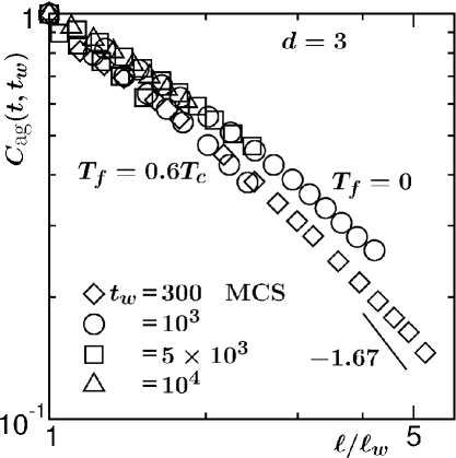
Figure 5: Log-log plots of the autocorrelation function, $C_{\rm ag}(t,t_{w})$, vs $\ell/\ell_{w}$, for $T_{f}=0$ and $0.6T_{c}$. For each value of $T_{f}$, results from multiple ages are presented. The solid line corresponds to a power-law decay, exponent for which is mentioned on the figure.

In Fig. 5 we show the plots of $C_{\rm ag}(t,t_{w})$, vs $\ell/\ell_{w}$, from $T_{f}=0$ and $0.6T_{c}$, on a log-log scale, for different values of $t_{w}$. Good collapse of data, for both the values of $T_{f}$, are visible over the whole range of the abscissa variable. This, in addition to establishing the scaling property of Eq. (5), implies the absence of the finite-size effects jia_suman ; jia_pre . On the issue of the finite size effects for the nonconserved Ising model, a previous study jia_suman showed that such effects become important only for $\ell>0.4L$. The length of our simulations were set in such a way that we are on the edge of this limit. For $T_{f}=0$, this can be appreciated from the $\ell$ vs $t$ data in the main frame of Fig. 3.

From a Gaussian auxiliary field ansatz, in the context of the time dependent Ginzburg-Landau model bray_phase , Liu and Mazenko (LM) liu constructed a dynamical equation for $C(\vec{r}_{1},t_{w};\vec{r}_{2},t)$. For $t\gg t_{w}$, from the solution of this equation, they obtained $\lambda\simeq 1.67$ in $d=3$. The solid line in Fig. 5 represents a power-law decay with the above mentioned value of the exponent. The simulation data, for both values of $T_{f}$, appear inconsistent with this exponent. Rather, the simulation results on the log-log scale exhibit continuous bending. Such bending may be due to the presence of correction to the power law decay at small values of $x$. Thus, more appropriate analysis is needed to understand these results.

In Fig. 6 we plot the instantaneous exponent liu ; huse_1986 ; jia_suman

$$\lambda_{i}=-\frac{d\ln C_{\rm ag}}{d\ln x},$$ (17)

as a function of $1/x$, for $T_{f}=0.6T_{c}$. A linear behavior is visible, extrapolation of which, to $x\rightarrow\infty$, leads to $\lambda\simeq 1.62$. The latter number follows the FH bound fisher_huse and is in good agreement with the theoretical prediction of LM liu . Such a linear trend provides an empirical full form for the autocorrelation function to be jia_suman

$$C_{\rm ag}=C_{0}{\exp\bigg{(}-\frac{B}{x}\bigg{)}}x^{-\lambda},$$ (18)

where $C_{0}$ and $B$ are constants. A finite-size scaling analysis jia_suman using this expression provided a value even closer to the LM one. Here note that there already exists henkel a full form, derived from the local scale invariance, for the decay of $C_{\rm ag}$ during coarsening in the ferromagnetic Ising model. Validity of this has been demonstrated in studies lorenz of $q(>2)$-state Potts model. Even though derived from a rigorous theoretical method, this expression contains a large number of unknowns. Thus, analyses of the simulation results by assuming this form is a tedius process. However, it will be an useful exercise to check how close an approximation Eq. (18) is to this form.

The decay of $C_{\rm ag}$, as seen in Fig. 5, for $T_{f}=0$ appears slower than that for $T_{f}=0.6T_{c}$. To confirm that, in Fig. 7 we plot the ratio $R$, between $C_{\rm ag}$ for $T_{f}=0.6T_{c}$ and $T_{f}=0$, on a log-log scale, vs $x$. Over the whole range of $x$, that covers pre- as well as post-crossover regimes for domain growth, the data exhibit power-law behavior that can be captured by a single exponent $\simeq 0.15$. This implies an absence of crossover in the decay of this quantity and $\lambda\simeq 1.5$, a number significantly smaller than that for $T_{f}=0.6T_{c}$. Whether or not the FH lower bound has actually been violated, such small value of $\lambda$ calls for further discussion and calculation of the structural properties.

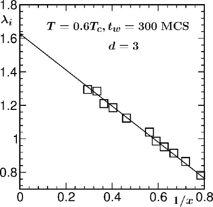
Figure 6: Plot of the instantaneous exponent, $\lambda_{i}$, vs $1/x$, for $T_{f}=0.6T_{c}$, with $t_{w}=300$ MCS. The solid line is a guide to the eyes.

Yeung, Rao and Desai (YRD) made a more general prediction of the lower bound yrd , viz.,

$$\lambda\geqslant\frac{d+\beta}{2},$$ (19)

where $\beta$ is the exponent yeung ; lubachev for the small wave-number ($k$) power-law enhancement of the structure factor (the Fourier transform of $C(r,t)$):

$$S(k)\sim k^{\beta}.$$ (20)

Here note that $S(k,t)$ has the scaling form (for a self-similar pattern) bray_phase

$$S(k,t)\equiv\ell^{d}\tilde{S}(k\ell),$$ (21)

where $\tilde{S}$ is a time independent master function. For nonconserved order parameter yrd , as in the present case, $\beta=0$. Thus the YRD lower bound in this case is same as the FH lower bound. The latter bound can as well be appreciated from the OJK expression for the general correlation function ojk ; puri in Eq. (I). This has the form

$$C(r;t,t_{w})=\frac{2}{\pi}\sin^{-1}\gamma,$$ (22)

with

$$\gamma=\bigg{(}\frac{2\sqrt{tt_{w}}}{t+t_{w}}\bigg{)}^{d/2}{\rm exp}\bigg{[}-\frac{r^{2}}{4D(t+t_{w})}\bigg{]}.$$ (23)

For $t=t_{w}$, this leads to Eq. (8). For $r=0$ and $t>>t_{w}$, Eq. (23) provides

$$C_{\rm ag}(t,t_{w})\sim\bigg{(}\frac{t}{t_{w}}\bigg{)}^{-d/4}.$$ (24)

For $\alpha=1/2$, the exponent in Eq. (24) provides $\lambda=d/2$, which coincides with the FH lower bound. Since the latter bound is embedded in Eq. (22) and the violation of it for $T_{f}=0$ is a possibility, it is instructive to calculate the structural quantities, viz., $C(r,t)$ and $S(k,t)$, given that Eq. (22) contains expressions for the latter quantities as well.

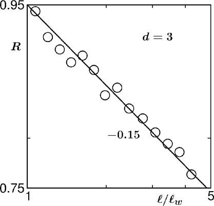
Figure 7: Log-log plot of the ratio, $R$, between the master curves for the autocorrelations at $T_{f}=0.6T_{c}$ and $0$, as a function of $x$.

In Fig. 8 we show a scaling plot of $C(r,t)$, vs $r/\ell$, for $T_{f}=0$, $\ell$ being extracted from Eq. (12). Nice collapse is visible for data from wide time range. Given that no crossover in $C(r,t)$ is observed and aging property is strongly related to the structure, it is understandable why a crossover in the autocorrelation is nonexistent. The continuous line in this figure is the OJK function bray_phase ; ojk ; puri of Eq. (8). There exists significant discrepancy between the analytical function and the simulation results. In the inset of this figure we plot the corresponding MC results for $T=0.6T_{c}$ which, on the other hand, shows nice agreement with Eq. (8). Here note that in $d=2$ such temperature dependence does not exist puri . For the sake of completeness, this we have demostrated in Fig. 9. Data from all the temperatures in this case are nicely described by the OJK function.

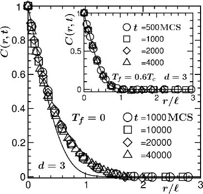
Figure 8: Scaling plot of the two-point equal time correlation functions from $T_{f}=0$. The distance along the abscissa has been scaled by the average domain sizes at different times from which data are presented. Inset: Same as the main frame, but for $T_{f}=0.6T_{c}$. In both the cases the solid curves represent the OJK form (see Eq. (8)).

In Fig. 10 we show a comparison between the structure factors from $T_{f}=0$ and $T_{f}=0.6T_{c}$, in $d=3$. The $k^{-4}$ line in this figure corresponds to the Porod law bray_phase ; puri ; porod for the long wave-number decay of $S(k,t)$, a consequence of scattering at sharp interfaces. Data from both the temperatures show reasonable consistency with this decay, even in intermediate range of $k$. For the sake of bringing clarity in the small $k$ region, we did not present the results for the whole range of $k$. Disagreement between the two cases is visible in the smaller wave-number region. This may provide explanation for the small value of $\lambda$ for $T_{f}=0$. For this purpose, below we provide a further discussion on the derivation of YRD. Starting from the equal-time structure factors at $t_{w}$ and $t$, YRD arrived at yrd

$$C_{\rm ag}(t,t_{w})\leq\ell^{d/2}\int_{0}^{2\pi/\ell}dkk^{d-1}S(k,t_{w})\tilde{S}(k\ell).$$ (25)

To obtain the lower bound, they used the small $k$ form for $S(k,t_{w})$, as quoted in Eq. (20). In Fig. 10 we see that, compared to $T_{f}=0.6T_{c}$, the the structure factor for $T_{f}=0$ starts decaying at a smaller value of $k$, providing an effective negative value for $\beta$. This is the reason for such a small value of $\lambda$.

Given that $T_{f}=0.6T_{c}$ lies above the roughening transition temperature $T_{R}$ ($\simeq 0.57T_{c}$), possibility exists corberi that the observed differences between kinetics at the two different values of $T_{f}$ may be related to this transition nolden . Our preliminary results for other values of $T_{f}$ ($<T_{R}$) are suggestive of this. However, more systematic study is needed. Here note that at the roughening transition the inteface thickness diverges. We mention here, most of the previous studies with Glauber glauber Ising model focused on $d=2$, for which there is no roughening transition. Nevertheless, question remains, why the crossovers, exhibited by the growth of domains and the decay of persistence, are missing in the structure and aging?

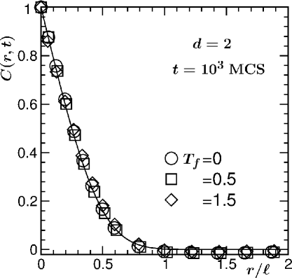
Figure 9: Scaled correlation functions from different $T_{f}$ in $d=2$. The continuous curve is the the OJK function of Eq. (8).

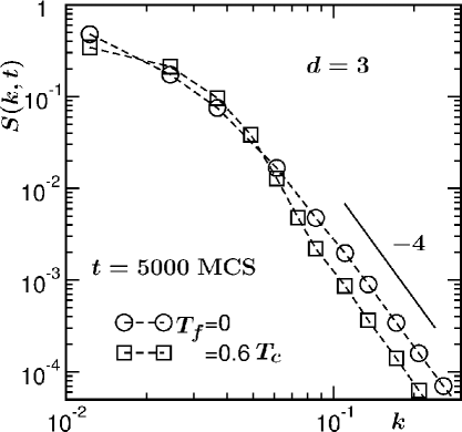
Figure 10: Plots of the structure factors, from $T_{f}=0$ and $0.6T_{c}$, vs $k$. The solid line represents the Porod law. For both the temperatures, we have presented results from $t=5000$.

IV Conclusion

We have studied kinetics of phase transition in $3D$ Ising model via the Glauber Monte Carlo simulations d_landau ; glauber , following quench from $T_{i}=\infty$ to $T_{f}=0$. Results are presented for domain growth, persistence probability, aging and pattern, all of which exhibit new features, compared to studies in $d=2$ and quenches to higher temperature for $d=3$. The time dependence of the average domain size shows consistency with the expected theoretical behavior only after an exceptionally long transient period saikat_pre ; corberi . This is reflected in the persistence probability saikat_pre . However, there is no such transient above the roughening transition.

The two-point equal time correlation function does not follow the Ohta-Jasnow-Kawasaki form ojk , derived for the nonconserved order-parameter dynamics with scalar order parameter. The latter form, however, is found to be consistent with the simulation data above the roughening transition temperature. Unlike the domain growth and persistence, we did not observe any time dependence (crossover) for this observable. This is reflected in the decay of the autocorrelation function. The latter quantity appears to have a power-law decay exponent marginally satisfying the Fisher-Huse lower bound. These results are at deviation with those from $d=2$ for which there is no roughening transition.

It will be important to understand the temperature dependence in all these quantities via more systematic studies. This may as well provide information on the deficiencies in the inputs for the derivation of the OJK function. One needs to check whether the roughening transition has any role to play with the Gaussian approximation, used in the calculation of the structure function. Furthermore, the reason for long transient in domain growth and persistence deserves attention. These we aim to address in future works.

References

- (1) A. Onuki, Phase Transition Dynamics, Cambridge University Press, Cambridge, UK (2002).
- (2) A.J. Bray, Adv. Phys. 51, 481 (2002).
- (3) S. Puri and V. Wadhawan (ed.), Kienetics of Phase Transitions (Boca Raton: CRC Press, 2009).
- (4) S.M. Allen and J.W. Cahn, Acta Metall. 27, 1085 (1979).
- (5) D.S. Fisher and D.A. Huse, Phys. Rev. B 38, 373 (1988).
- (6) F. Corberi, E. Lippiello and M. Zannetti, Phys. Rev. E 74, 041106 (2006).
- (7) F. Liu and G.F. Mazenko, Phys. Rev. B 44, 9185 (1991).
- (8) S.N. Majumdar and D.A. Huse, Phys. Rev. E 52, 270 (1995).
- (9) C. Yeung, M. Rao and R.C. Desai, Phys. Rev. E 53, 3073 (1996).
- (10) M. Henkel, A. Picone and M. Pleimling, Europhys. Lett. 68,191 (2004).
- (11) A.J. Bray, S.N. Majumdar and G. Schehr, Adv. Phys. 62, 225 (2013).
- (12) S.N. Majumdar, C. Sire, A.J. Bray and S.J. Cornell, Phys. Rev. Lett. 77, 2867 (1996).
- (13) S.N. Majumdar, A.J. Bray, S.J. Cornell and C. Sire, Phys. Rev. Lett. 77, 3704 (1996).
- (14) B. Derrida, Phys. Rev. E 55, 3705 (1997).
- (15) D. Stauffer, Int. J. Mod. Phys. C 8, 361 (1997).
- (16) G. Manoj and P. Ray, Phys. Rev. E 62, 7755 (2000).
- (17) B. Derrida, A.J. Bray and C. Godrèche, J. Phys. A 27, L357 (1994).
- (18) D. Stauffer, J. Phys. A 27, 5029 (1994).
- (19) D.P. Landau and K. Binder, A Guide to Monte Carlo Simulations in Statistical Physics, Cambridge University Press, Cambridge (2009).
- (20) T. Ohta, D. Jasnow and K. Kawasaki, Phys. Rev. Lett. 49, 1223 (1982).
- (21) J. Midya, S. Majumder and S.K. das, J. Phys. : Condens. Matter 26, 452202 (2014).
- (22) T. Blanchard, L.F. Cugliandolo and M. Picco, J. Stat. Mech. P12021 (2014).
- (23) S. Chakraborty and S.K. Das, European Phys. J. B 88, 160 (2015).
- (24) J.G. Amar and F. Family, Bull. Am. Phys. Soc. 34, 491 ͑(1989͒).
- (25) J.D. Shore, M. Holzer, and J.P. Sethna, Phys. Rev. B 46, 11376 ̵͑(1992͒).
- (26) S. Cueille and C. Sire, J. Phys. A 30, L791 (1997).
- (27) F. Corberi, E. Lippiello and M. Zannetti, Phys. Rev. E 78, 011109 (2008).
- (28) S. Chakraborty and S.K. Das, Phys. Rev. E 93, 032139 (2016).
- (29) R.J. Glauber, J. Math. Phys. 4, 294 (1963).
- (30) S. Majumder and S.K. Das, Phys. Rev. E 81, 050102 (2010).
- (31) D.A. Huse, Phys. Rev. B, 34, 7845 (1986).
- (32) M.E. Fisher, in Critical Phenomena, edited by M.S. Green (Academic, London, 1971).
- (33) D.W. Heermann, L. Yixue and K. Binder, Physica A 230, 132 (1996).
- (34) S.K. Das, S. Roy, S. Majumder and S. Ahmad, EPL 97, 66006 (2012).
- (35) J. Midya, S. Majumder and S.K. das, Phys. Rev. E 92, 022124 (2015).
- (36) E. Lorenz and W. Janke, EPL 77, 10003 (2007).
- (37) C. Yeung, Phys. Rev. Lett. 61, 1135 (1988).
- (38) S.N. Majumdar, D.A. Huse and B.D. Lubachevsky, Phys. Rev. Lett. 73, 182 (1994).
- (39) G. Porod, in Small-Angle X-ray scattering, edited by O. Glatter and O. Kratky, Academic press, New York, 42 (1982).
- (40) H. van Beijeren and I. Nolden, in Structures and Dynamics of Surfaces II: Phenomena, Models and Methods, Topics in Current Physics vol. 43, edited by W. Schommers and P. von Blanckenhagen (Berlin: Springer, 1987).