KCL-MTH-16-05

KCL-PH-TH-2016-39

The Two-Parameter Brane $\sigma$-model: $M^{*}$, $M^{\prime}$ solutions and $M$-theory solutions dependent on exotic coordinates
Paul P. Cook
Department of Mathematics, King’s College London
Strand, London WC2R 2LS, UK
and
Sarben Sarkar
Theoretical Particle Physics and Cosmology Group, Department of Physics, King’s College London
Strand, London WC2R 2LS, UK

We investigate two-parameter solutions of $\sigma$-models on two dimensional symmetric spaces contained in $E_{11}$. Embedding such $\sigma$-model solutions in space-time gives solutions of $M^{*}$ and $M^{\prime}$-theory where the metric depends on general travelling wave functions, as opposed to harmonic functions typical in general relativity, supergravity and M-theory. Weyl reflection allows such solutions to be mapped to M-theory solutions where the wave functions depend explicitly on extra coordinates contained in the fundamental representation of $E_{11}$.

1 Introduction

Fifteen years ago, just after the turn of the century, the Kac-Moody algebra $E_{11}$ was conjectured to encode symmetries of M-theory in its eleven dimensional form [1]. Around the same time it was shown that the dynamics of eleven-dimensional supergravity near a space-like singularity are encoded in a one-parameter $\sigma$-model invariant under the action of a coset group associated with a Kac-Moody algebra $E_{10}$ [2, 3]. The Lagrangian of the sigma-model is defined in terms of scalar fields on a coset space and solutions to the equations of motion define a null geodesic on a symmetric space which may be used to reconstruct space-time solutions. In the work of [2, 3] the fields were parameterised by time, a truncation sensible in the vicinity of a space-like singularity, but at the expense of equivalent roles for the spatial and temporal coordinates. The Lorentz symmetry was re-introduced into the $\sigma$-model construction in [4] and used to construct solutions dependent on space-time from $\sigma$-models on symmetric spaces embedded within the Kac-Moody algebra $E_{11}$. This formulation of constructing space-time solutions from sub-algebras of a Kac-Moody algebra came to be known as the ‘brane $\sigma$-model’ and was used more recently to reconstruct bound state solutions in $M$-theory and string theory [5, 6] following observations made in [7]. In all these cases the solutions of supergravity, superstring theory and $M$-theory that were constructed were encoded in the path traversed by a massless particle on the coset space.

The symmetric spaces used in these brane $\sigma$-models are constructed using the Kac-Moody algebras $E_{10}$ and $E_{11}$. These algebras have long been argued to encode hidden symmetries of supergravity relevant to $M$-theory [8, 1] and the coset construction provides a dictionary relating the path of a massless particle on a coset to brane solutions in space-time. The $\sigma$-model action on the coset for a massless particle is a simpler and, arguably, more fundamental setting to investigate $M$-theory and the high-energy description of space-time. Consequently it is of interest to consider simple extensions of the massless particle motion on cosets of subgroups of $E_{10}$ and $E_{11}$. In this paper, instead of the motion of a massless particle, we consider the motion of a string on the cosets of subgroups of $E_{11}$.

The simple symmetric spaces related to brane solutions are two-dimensional manifolds and our aim is to investigate two-parameter solutions on these manifolds and consider their embedding in space-time. The symmetric spaces we consider will be pseudo-Riemannian and a consequence of developing two-parameter solutions is that, upon embedding the parameters in space-time, the transverse space to the “brane” world-volume will contain both timelike and spacelike coordinates. The resulting two-parameter metrics and gauge-fields will be solutions of $M^{*}$ and $M^{\prime}$ theories [9]. The $E_{11}$ conjecture leads to an enhancement of $M$-theory which contains both $M^{*}$ and $M^{\prime}$-theories [10]: sub-algebras of $E_{11}$ related to the three theories are mapped into each other under $E_{11}$ Weyl reflections. As solutions of $\sigma$-models are preserved under Weyl reflections this leads to the question: what are the two-parameter solutions of $M^{*}$ and $M^{\prime}$-theories mapped to in $M$-theory? We will argue that the solutions are $M$-theory solutions which depend on the extra $E_{11}$ coordinates $y_{\mu_{1}\mu_{2}}$, $z_{\mu_{1}\mu_{2}\mu_{3}\mu_{4}\mu_{5}}$, $w_{\mu_{1}\mu_{2}\mu_{3}\mu_{4}\mu_{5}\mu_{6}\mu_{7}|\nu}$, $w_{\mu_{1}\mu_{2}\mu_{3}\mu_{4}\mu_{5}\mu_{6}\mu_{7}\mu_{8}}$ and so on which are contained in the first fundamental, or $l_{1}$, representation of $E_{11}$ [11]. These are the same extra coordinates central to the internal symmetries of double field theory [12, 13] and exceptional field theory [14] which were first introduced in [15, 16]. The extra coordinates will require an extension of the brane $\sigma$-model which we will discuss in our concluding remarks.

It should be mentioned that there is another aspect of hidden symmetries and duality, based on the study of Einstein’s theory of general relativity, which has stimulated the study of cosets of subgroups of $E_{10}$ and other Kac-Moody algebras. In an early work Buchdahl [17] noticed a transformation between two static solutions of Einstein’s equations which can now be interpreted as T-duality. Subsequently Ehlers [18] uncovered a symmetry which generated solutions of Einstein’s equations. A significant breakthrough came with the work of Geroch [19, 20] who extended Ehlers’ $SL(2,\mathbb{R})$ symmetry to the (infinite dimensional) affine $SL(2,\mathbb{R})$ Kac-Moody algebra for axi-symmetric stationary solutions. These ideas were developed and used in general relativity for the generation of solutions. Such hidden symmetries were later discovered to be present in supergravity. In particular for $N=8$ supergravity there is a continuous global group $E{{}_{7(7)}}$ which is a symmetry [21, 22]. ($E{{}_{7(7)}}$ is a non-compact version of $E_{7}$; it is spontaneously broken in supergravity.) These observations led to the study of the groups, and their generalisations, encoding the symmetries. The symmetry groups above were found for special classes of solutions of Einstein’s equation. There has been a quest for larger symmetries associated with the full theory. For Einstein’s equations generically there are singularities in four space-time dimensions. For a space-like singularity Belinskii, Khalitnikov and Lifshitz pointed out that near such a singularity, the spatial metrics at each spatial point are decoupled and they satisfy non-linear second order ordinary differential equations in time. Misner [23, 24] initiated the study of such space-like singularities using Hamiltonian theory and this led to a billiard description [3] in hyperbolic space. Pure gravity billiards have an underlying hidden Kac-Moody algebra as a symmetry. Such symmetries can be studied with the help of geodesic sigma-models. It is in the consideration of $\sigma$-models that our approach overlaps with the billiards approach.

We will now give a more detailed description of the brane $\sigma$-model and the $E_{11}$ conjecture. The one-parameter brane $\sigma$-model was developed in [4] as a way to associate a covariant Lagrangian density with sub-algebras of the very-extended Kac-Moody algebra $E_{11}$. The model gives a dictionary in which brane solutions of supergravity are identified with the worldline of a particle moving on a null geodesic on the coset manifold $\frac{SL(2,\mathbb{R})}{SO(1,1)}$ embedded within $\frac{E_{11}}{{\cal K}(E_{11})}$, where the algebra ${\cal K}(E_{11})$ is the part of the algebra $E_{11}$ invariant under an involution determined by the signature of space-time and the sign of the four-form in the supergravity action. The dictionary defines the embedding of the null geodesic on the symmetric space into space-time; for brane solutions the parameter on the worldline is identified with a single transverse direction. In this manner the brane $\sigma$-model reconstructs a one-dimensional action for a single brane solution from a sub-algebra of $E_{11}$ and the one-dimensional action may be oxidised to the bosonic supergravity action in eleven-dimensions where only diagonal components of the metric $g_{\mu\nu}$ and the six related components of the three-form $A_{\mu\nu\rho}$ (defined by fixed $\mu$, $\nu$ and $\rho$) are non-trivial. The brane $\sigma$-model has been used to construct bound state solutions, identified in [7], associated with null geodesics on the symmetric spaces $\frac{G}{{\cal K}(G)}$ where $G$ is a finite Lie group, larger than $SL(2,\mathbb{R})$ such that $G\subset E_{11}$ [5], these techniques were used to find further bound states in string theory in [6] and in dual graviton theories in [25]. All of the solutions found in this way are stationary solutions. By introducing a second parameter to the brane $\sigma$-model on the symmetric space $\frac{SL(2,\mathbb{R})}{SO(1,1)}$, time-dependent solutions will be constructed, albeit solutions to $M^{*}$ and $M^{\prime}$-theories. The algebra $E_{11}$ was conjectured to encode the symmetries underlying $M$-theory in [1], it was made manifest there by applying the Borisov-Ogievetsky construction [26] used to generate the diffeomorphism algebra of gravity (by finding the closure of the conformal group and the Poincaré group) to find the closure of the conformal group with the bosonic part of the supergravity algebra in eleven dimensions. Its appearance in dimensional reduction was anticipated [8] as the end of the $E_{11-d}$ sequence of ‘hidden’ symmetries that act on the scalar fields of a Kaluza-Klein reduction of bosonic supergravity in eleven dimensions to $d$-dimensions. In other words, $E_{11}$ was expected to be related to the theory in zero dimensions, but it was conjectured by West [1] that it was already present in an eleven dimensional theory which was an extension of supergravity called $M$-theory. It was subsequently shown that $E_{11}$ has a very simple relationship to the type IIA and type IIB string theories: the gauge fields of the bosonic parts of these string theories which source the string, the $Dp$-branes as well as the NSNS fields all emerge from the representation theory of $E_{11}$ [27]; the brane solutions of the string theories as well $M$-theory are all straightforwardly encoded in a solution-generating group element [28] and basic properties relating fundamental dimensionful quantities in each theory have also been derived from the Kac-Moody algebra [1]. There is now a wealth of literature supporting the $E_{11}$ conjecture; it has been used in a variety of settings. There has also been a great deal of work investigating the over-extended algebra $E_{10}\subset E_{11}$ whose importance in dynamics in the vicinity of cosmological singularities [2] was the motivation for first investigating $\sigma$-models in this context: brane solutions were constructed and $E_{10}$ has been used to construct the fermionic terms expected in supergravity. For a review of $E_{10}$ and cosmological billiards see [29]. In this paper we will work with $E_{11}$.

The $E_{11}$ conjecture can be stated as the idea that the fields of $M$-theory parameterise a symmetric space $\frac{E_{11}}{{\cal{K}}(E_{11})}$ and the coordinates of space-time parameterise the first fundamental, or $l_{1}$, representation of $E_{11}$. The solutions describing single and bound states of branes which have been constructed using the one-parameter $\sigma$-model have given fields which parameterise finite dimensional symmetric spaces embedded in $\frac{E_{11}}{{\cal{K}}(E_{11})}$ and depend on only one parameter. That parameter has been identified with one of the eleven space-time coordinates $x^{\mu}$ via a supergravity dictionary. The procedure, successful though it has been, has left questions about the role of the topology of $\frac{E_{11}}{{\cal{K}}(E_{11})}$, a geometric origin in space-time of the symmetric space and the dependence on the extra coordinates. Let us describe these three problems in more detail:

1. The Borel or upper-triangular gauge is used for group elements when constructing the Lagrangians in the brane $\sigma$-models. It was observed in [10] that the use of this gauge results in the loss of closed compact cycles in the coset spaces, effectively reducing the topology of the coset $\frac{SL(2,\mathbb{R})}{SO(1,1)}$ from $S^{1}\times\mathbb{R}^{1}$ to $\mathbb{R}^{2}$. Information related to closed loops within the coset is lost by using the Borel gauge for the massless particle, however by considering the motion of closed strings which surround the closed cycles of the coset the full group structure may be able to play a role in the space-time theory.

2. The possibility of constructing solutions dependent upon two parameters, one spacelike and the other timelike on the coset raises interesting questions for the embedding of such cosets in space-time. The supergravity dictionary used for the massless particle model associates the single parameter of the solution on the coset with the radial coordinate in a space-time with rotational symmetry group $SO(D-p-1)$ transverse to a p-brane solution. The string solutions we will describe here depend on two-coordinates $\sigma$ and $\tau$ which may elucidate the geometrical meaning of the coset within space-time.

3. The identification of the parameter in the brane $\sigma$-model with a coordinate $x^{\mu}$ of space-time informs the embedding of the $\sigma$-model solution in space-time. At the same time it precludes the appearance of solutions which depend upon the extra coordinates of space-time necessary for $E_{11}$. The natural extension of considering particle worldlines and string worldsheets on symmetric spaces within $E_{11}$ is to consider $p$-brane worldvolumes where the dimension of the symmetric space is $p$. However this invites questions as to how this will be embedded in space-time when $p>11$ (e.g. for the symmetric space $\frac{SL(5,\mathbb{R})}{SO(1,4)}$ which is a 14-dimensional manifold). It will be necessary in such cases to invoke the extra coordinates of $E_{11}$, however there is no supergravity dictionary to inform the construction of these solutions. The two-parameter brane $\sigma$-model describes $M$-theory solutions dependent upon extra coordinates, hence its construction will shed some light on solutions dependent on extra space-time coordinates. In appendix B we will show that starting point for the study of gravity in the vicinity of a space-like symmetry is replicated in a natural way if the $3$-metric obtained in a foliation of space-time depends on a space-like as well as a time-like parameter.

The work in the present paper will construct two-parameter solutions, and is an initial step towards addressing the last two points listed above. To directly address the first point requires a closed string worldsheet wrapping the cycle of $\frac{SL(2,\mathbb{R})}{SO(1,1)}$, which is not possible using the Borel gauge adopted in this paper. However such a construction would allow the topology of $\frac{E_{11}}{{\cal{K}}(E_{11})}$ to play a role in the space-time fields.

In section 2 we will review the construction of $\frac{1}{2}$-BPS brane solutions of supergravity as null geodesic motions of a particle on cosets of $SL(2,\mathbb{R})$ embedded in $E_{11}$. Our aim in this section will be to familiarise the reader with all aspects of the construction of the one-parameter brane $\sigma$-model before presenting the two-parameter $\sigma$-model in section 3. We will present simple solutions to this model dependent on two-parameters, some of which are only solutions in two-dimensions, but other more general solutions which are described by wavefunctions. In section 4 we will embed the two-parameter solutions into space-times with multiple time coordinates and show some examples of solutions to bosonic $M^{*}$-theory and $M^{\prime}$-theory described in terms of wavefunctions. We will apply Weyl reflections to map these solutions into $M$-theory and see that they depend on extra coordinates. We will conclude in section 5.

2 Brane solutions and the brane $\sigma$-model

In this section we will review the one-parameter brane $\sigma$-models and show how given an involution $\Omega$ defined on the algebra of $E_{11}$ we may define the “group” ${\cal K}(E_{11})$ whose algebra is fixed under $\Omega$. We will then review how any real root of $E_{11}$ may be associated with a sigma-model on the symmetric spaces $\frac{SL(2,\mathbb{R})}{SO(1,1)}$ or $\frac{SL(2,\mathbb{R})}{SO(2)}$. In the former case the solutions of the equations of motion encode electric brane solutions of $M$-theory, or one of its counterparts $M^{*}$ or $M^{\prime}$-theory [9], while there are no real solutions to the equations of motion in the latter case. Our principal example will be the solution of the $\frac{SL(2,\mathbb{R})}{SO(1,1)}$ model associated with the exceptional root ${\underline{\alpha}}_{11}$ of $E_{11}$, which encodes the $M2$-brane of $M$-theory. We commence by defining the involution $\Omega$ which leaves the algebra of ${\cal{K}}(E_{11})$ invariant before constructing the $\sigma$-models on $\frac{SL(2,\mathbb{R})}{SO(1,1)}$ and $\frac{SL(2,\mathbb{R})}{SO(2)}$. The involution $\Omega$ encodes the signature of the background space-time. The equations of motion on each symmetric space will be presented, and it will be observed that the $\sigma$-model on the first space has real solutions which will be embedded into space-time while the $\sigma$-model on the second space does not possess real solutions.

2.1 The signature of space-time.

The algebra $E_{11}$ is infinite dimensional, and is associated with the extension of eleven-dimensional supergravity by singling out an $SL(11,\mathbb{R})$ sub-algebra. This sub-algebra is formed of the nodes $1,2\ldots 10$ labelled on the Dynkin diagram of $E_{11}$ as depicted in figure 1 and sometimes called the gravity line.

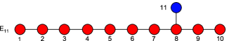
Figure 1: The Dynkin diagram of $E_{11}$, the line of red nodes indicate the Dynkin diagram of $SL(11,\mathbb{R})$ associated with the eleven dimensional space-time.

The decomposition of the algebra $E_{11}$ with respect to the gravity line gives an infinite set of tensor representations of $SL(11,\mathbb{R})$. Any root ${\underline{\beta}}$ within the root space of $E_{11}$ may be written as a sum of simple, positive roots: ${\underline{\beta}}=\sum_{i=1}^{11}m_{i}{\underline{\alpha}}_{i}$ and the decomposition into representations of $SL(11,\mathbb{R})$ may be understood as splitting the root ${\underline{\beta}}$ into a weight in the weight space of $SL(11,\mathbb{R})$, denoted ${\underline{\Lambda}}$, and a part ${\underline{x}}$ orthogonal to the weights of $SL(11,\mathbb{R})$, i.e. ${\underline{\beta}}={\underline{\Lambda}}+m_{11}{\underline{x}}$. The coefficient $m_{11}$ is called the level and labels sets of representations of $SL(11,\mathbb{R})$ defined by a lowest (equivalent to the highest weight labelling) weight ${\underline{\Lambda}}$. For example at level $m_{11}=0$, we find the roots of $SL(11,\mathbb{R})$, at level one ($m_{11}=1$) we find an antisymmetric three-tensor representation $R^{a_{1}a_{2}a_{3}}$, at level two we have an antisymmetric six-tensor $R^{a_{1}\ldots a_{6}}$, at level three we find a mixed symmetry tensor $R^{a_{1}\ldots a_{8}|b}$ and so on.

The signature of space-time is derived from the quadratic form invariant under $SO(1,10)$. The algebra of this group is invariant under the (temporal) involution $\Omega$ which acts on the positive generators $E_{i}$ of $\mathfrak{sl}(11,\mathbb{R})$ as

$$\Omega(E_{i})=-\epsilon_{i}(F_{i}),$$ (1)

where $F_{i}$ are the negative generators and $\epsilon_{i}=\pm 1$ where $i\in\{1,2,\ldots 10\}$. The sub-algebra of $\mathfrak{sl}(11,\mathbb{R})$ invariant under $\Omega$ is $\mathfrak{so}(p,q)$ where $p,q\in\mathbb{Z}_{0}^{+}$ such that $p+q=11$, having generators $Q_{i}\equiv E_{i}-\epsilon_{i}F_{i}$ (where there is no summation over the repeated indices). The remainder of the algebra (the anti-fixed set of generators under $\Omega$) consists of $P_{i}\equiv E_{i}+\epsilon_{i}F_{i}$ and the generators of the Cartan sub-algebra $H_{i}$. For example if $\epsilon_{1}=\epsilon_{2}=\ldots\epsilon_{10}=1$ then the sub-algebra fixed under $\Omega$ is spanned by the generators $Q_{i}\equiv E_{i}-F_{i}$, or in other words $\mathfrak{so}(11)$. Alternatively if $\epsilon_{1}=-1$, while $\epsilon_{2}=\ldots\epsilon_{10}=1$ the fixed sub-algebra is $\mathfrak{so}(1,10)$. By appropriate choice of $\epsilon_{i}$ the sub-algebra $\mathfrak{so}(t,11-t)$ may be constructed. Extending the action of $\Omega$ to the generator $R^{9\,10\,11}$ associated with the exceptional node of the $E_{11}$ Dynkin diagram (the blue eleventh node shown in figure 1) as $\Omega(R^{9\,10\,11})=\epsilon_{11}R_{9\,10\,11}$, one may define ${\cal K}(E_{11})$ as the exponentiation of the sub-algebra invariant under the involution $\Omega$. The role of $\epsilon_{11}$ is to control the sign in front of the kinetic term for the three-form gauge field in the supergravity action [30]. In summary $\Omega$ is defined by a choice of eleven numbers $\epsilon_{i}$ and encodes the space-time signature and the sign of the kinetic term in the action.

It was shown in [30] that the signature of space-time defined by the choice of $\Omega$ is not invariant under the Weyl reflections of $E_{11}$. This may be understood as follows: the signature of space-time depends on the action of $\Omega$ on the generators of $\mathfrak{sl}(11,\mathbb{R})$ given by the gravity line (the red nodes numbered from one to ten in figure 1), but under a Weyl reflection the generators associated with the gravity line may be mapped to another $\mathfrak{sl}(11,\mathbb{R})$ sub-algebra within $E_{11}$ and vice-versa, so that the gravity line is formed of a different set of $\mathfrak{sl}(11,\mathbb{R})$ generators before and after a Weyl reflection. Consequently the sub-algebra of the gravity line algebra which is invariant under $\Omega$ may change under a Weyl reflection. For example, commencing with a choice of $\Omega$ which leaves $\mathfrak{so}(1,10)$ fixed within the gravity line algebra following an $E_{11}$ Weyl reflection the gravity line sub-algebra fixed by $\Omega$ may be one of $\mathfrak{so}(1,10)$, $\mathfrak{so}(2,9)$, $\mathfrak{so}(5,6)$, $\mathfrak{so}(6,5)$, $\mathfrak{so}(9,2)$ or $\mathfrak{so}(10,1)$ [30]. This potential change of signature highlights the unnatural manner in which $E_{11}$ is associated with an eleven-dimensional space-time by an essentially arbitrary choice of $\mathfrak{sl}(11,\mathbb{R})$ sub-algebra. It would be more natural to consider $E_{11}$ as the symmetries of a theory on an infinite dimensional space-time with the background isometry group ${\cal K}(E_{11})$. A Weyl reflection in such a setting would leave the isometry group unaltered and would map active fields in one sector to another, preserving solutions. With the restriction to an eleven dimensional space-time the effect of a Weyl reflection is to change the signature of space-time while preserving solutions between theories.

While $\epsilon_{i}$ for $i=1,\ldots 10$ define the signature of space-time, $\epsilon_{11}$ is associated with the sign of the four-form kinetic term [30]. We will adopt the following conventions for the gravity-matter action associated with low levels of $E_{11}$ and a choice of involution $\Omega$,

$$S=\int R\star 1-(-1)^{(\epsilon_{0}+<{\underline{f}},{\underline{\gamma}}>)}\frac{1}{2}F_{\alpha_{11}}\wedge\star F_{\alpha_{11}}+\ldots$$ (2)

where $\epsilon_{0}\equiv 1$ if $x^{1}$ is a temporal coordinate and $\epsilon_{0}\equiv 0$ if $x^{1}$ is a spatial coordinate and ${\underline{\gamma}}\equiv{\underline{\alpha}}_{2}+{\underline{\alpha}}_{4}+{\underline{\alpha}}_{6}+{\underline{\alpha}}_{8}+{\underline{\alpha}}_{10}+{\underline{\alpha}}_{11}$; the ellipsis denotes other terms including the Chern-Simons term and generalisations of supergravity; and ${\underline{f}}$, known as the signature function and introduced in [30], is a function on the weight space of $E_{11}$ defined from the involution $\Omega$ by

$$\epsilon_{k}=e^{i\pi<{\underline{\alpha}}_{k},{\underline{f}}>}$$ (3)

where upon writing ${\underline{f}}\equiv\sum p_{i}{\underline{\lambda}}_{i}$, ${\underline{\lambda}}_{i}$ are the fundamental weights of $E_{11}$, we have $\epsilon_{k}=e^{i\pi p_{k}}$ and as $\epsilon_{k}\in\{0,1\}$ then $p_{k}\in\{0\mod 2,1\mod 2\}$. The Weyl reflections in real roots ${\underline{\beta}}$ of $E_{11}$ denoted $W_{{\underline{\beta}}}$ and defined by

$$W_{{\underline{\beta}}}({\underline{\alpha}})={\underline{\alpha}}-2\frac{<{\underline{\alpha}},{\underline{\beta}}>}{<{\underline{\beta}},{\underline{\beta}}>}{{\underline{\beta}}}$$ (4)

map the signature function from ${\underline{f}}$ to $\hat{f}\equiv W_{{\underline{\beta}}}({\underline{f}})$. This has the consequence of not only changing the signature of space-time but also the sign of the kinetic term in the action in equation (2). The involution $\Omega$ and hence the algebra of ${\cal K}(E_{11})$, or equivalently the signature function ${\underline{f}}$, is the first ingredient which must be specified before the brane $\sigma$-model may be constructed.

2.2 The one-parameter brane $\sigma$-model

For $G$, a semisimple Lie group embedded in $E_{11}$, $\sigma$-models constructed on the symmetric space $\frac{G}{{\cal K}(G)}$ have solutions which encode half-BPS brane solutions [4] and bound states of these brane solutions [7, 5, 6]. We restrict our attention in this paper to single brane solutions which correspond to identifying $G=SL(2,\mathbb{R})$ embedded in $E_{11}$. The truncation of the algebra $E_{11}$ to $\mathfrak{sl}(2,\mathbb{R})$ gives an associated truncation of the algebra of ${\cal K}(E_{11})$ to ${\cal K}(SL(2,\mathbb{R}))$ which is defined using the involution $\Omega$ on $E_{11}$. Taking $G=SL(2,\mathbb{R})$ whose single positive root ${\underline{\beta}}$ is a real root in the root lattice of $E_{11}$, ${\cal K}(G)$ is either $SO(2)$ or $SO(1,1)$. Given a signature function ${\underline{f}}$ then if $<{\underline{f}},{\underline{\beta}}>=1\mod{2}$ then ${\cal K}(G)=SO(1,1)$, while if $<{\underline{f}},{\underline{\beta}}>=0\mod{2}$ then ${\cal K}(G)=SO(2)$ [30]. We will observe in the construction of the $\sigma$-models how the sign choices of the kinetic term of the action in eleven dimensions above are related to the signs appearing in the one-dimensional action of the $\sigma$-models.

2.2.1 The Lagrangian density

The one-parameter $\sigma$-model has an action which is invariant under the symmetries of the coset $\frac{G}{{\cal K}(G)}$ and is defined by

$$S=\int d\xi\,{\cal L}$$ (5)

where $\xi$ is a single coordinate on the coset manifold on which the Lagrangian density ${\cal L}$ depends. The Lagrangian density is defined in terms of an inner product by

$${\cal L}=\eta^{-1}(P_{\mu}|P_{\mu})$$ (6)

where $P_{\mu}$ is derived by decomposing the Maurer-Cartan form $\nu\equiv dgg^{-1}$ for $g\in G$ as follows

$$\nu_{\mu}=(\partial_{\mu}g)g^{-1}=P_{\mu}+Q_{\mu}\in\mathfrak{g},$$ (7)

the inner product is the Cartan-Killing form, the generators denoted $Q_{\mu}$ are in the algebra of ${\cal K}(G)$, $P_{\mu}$ are the complementary generators in the Lie algebra of $G$ and the field $\eta$ is included to guarantee the reparameterisation invariance of the action $S$.

The Lagrangian density ${\cal L}$ is invariant under the symmetry transformations of the coset. Specifically the global transformation

$$g\rightarrow gg_{0}$$ (8)

where $g_{0}$ is independent of coordinates on the coset manifold leaves the Maurer-Cartan form unchanged:

$$\nu_{\mu}\rightarrow\partial_{\mu}(gg_{0})(gg_{0})^{-1}=\nu_{\mu}.$$ (9)

While the transformation under the local sub-group element $k(x^{\mu})\in K(G)$ given by

$$g\rightarrow kg$$ (10)

leaves the Lagrangian density ${\cal L}$ unchanged as

$$\nu_{\mu}\rightarrow\partial_{\mu}(kg)(kg)^{-1}=\partial_{\mu}(k)k^{-1}+k\nu_{\mu}k^{-1}$$ (11)

hence

$$P_{\mu}\rightarrow kP_{\mu}k^{-1}\qquad\mbox{and}\qquad Q_{\mu}\rightarrow kQ_{\mu}k^{-1}+\partial_{\mu}(k)k^{-1},$$ (12)

which leaves ${\cal L}$ unchanged. We now construct the Lagrangians for $G=SL(2,\mathbb{R})$.

2.3 The $\frac{SL(2,\mathbb{R})}{SO(1,1)}$ brane $\sigma$-model.

Let $g\in\frac{SL(2,\mathbb{R})}{SO(1,1)}$ be the coset representative written, in the Borel gauge (upper triangular gauge), in terms of $H$, the Cartan sub-algebra element of the algebra $sl(2,\mathbb{R})$ and $E$, the positive generator of $sl(2,\mathbb{R})$, as follows:

$$g=\exp(\phi H)\exp(CE)$$ (13)

where $\phi\equiv\phi(\tau,\sigma)$ and $C\equiv C(\tau,\sigma)$ and $\tau$ and $\sigma$ are local coordinates on the manifold chosen such that the local metric in these coordinates is Minkowskian with $\tau$ being a timelike coordinate and $\sigma$ spacelike.The single coordinate $\xi$ of the one-dimensional coset model action will be a function of $\sigma$ and $\tau$ singled out by the equations of motion. $H$ and $E$ are simply represented by two-by-two matrices:

$$H=\left(\begin{array}[]{cc}1&0\\ 0&-1\end{array}\right)\qquad\mbox{and}\qquad E=\left(\begin{array}[]{cc}0&1\\ 0&0\end{array}\right).$$ (14)

Hence

$$g=\left(\begin{array}[]{cc}e^{\phi}&e^{\phi}C\\ 0&e^{-\phi}\end{array}\right)$$ (15)

and therefore

$$\nu_{\mu}=\partial_{\mu}\phi H+\partial_{\mu}C\exp(2\phi)E.$$ (16)

The $so(1,1)$ sub-algebra is the part of $sl(2,\mathbb{R})$ which is invariant under the involution $\Omega$ defined by $\Omega(H)=-H$ and $\Omega(E)=F$ where $F\equiv E^{T}$ is the negative (lower triangular) generator of $sl(2,R)$. The sub-algebra of $so(1,1)$ contains a single generator $q=\frac{1}{2}(E+F)$, the remainder of the algebra of $sl(2,R)$ is spanned by $H$ and $p\equiv\frac{1}{2}(E-F)$. We have normalised $q$ and $p$ so that $E=q+p$. We have

$$\nu_{\mu}=\partial_{\mu}\phi H+\partial_{\mu}C\exp(2\phi)(p+q)\equiv P_{\mu}+Q_{\mu}$$ (17)

and

$$P_{\mu}=\left(\begin{array}[]{cc}\partial_{\mu}\phi&\frac{1}{2}e^{(2\phi)}\partial_{\mu}C\\ -\frac{1}{2}e^{(2\phi)}\partial_{\mu}C&-\partial_{\mu}\phi\end{array}\right).$$ (18)

This gives us the following Lagrangian density

$${\cal L}=\eta^{-1}(2(\partial\phi)^{2}-\frac{1}{2}e^{4\phi}(\partial C)^{2})$$ (19)

whose equations of motion are

$$\partial^{2}\phi+\frac{1}{2}(\partial C)^{2}e^{4\phi}=0\,,\quad\partial_{\mu}(\partial^{\mu}Ce^{4\phi})=0\quad\mbox{and}\quad(\partial\phi)^{2}-\frac{1}{4}e^{4\phi}(\partial C)^{2}=0.$$ (20)

These are the equations of motion for $\phi$, $C$ and $\eta$ resepectively.

The final equation of motion above may be written as $(P_{\mu}|P_{\mu})=0$ and hence the path of $P_{\mu}$ described on the group manifold will be a null geodesic on the coset. The solution will therefore be described by a single parameter, which we have chosen to be $\xi$. Let us see how the solution emerges.

As $\partial_{\mu}(\partial^{\mu}Ce^{4\phi})=0$, then $(\partial^{\mu}C)e^{4\phi}=\epsilon^{\mu\nu}\partial_{\nu}A$ where $A\equiv A(\sigma,\tau)$. In components this gives

$$(\partial^{\sigma}C)e^{4\phi}=\partial_{\tau}A\quad\mbox{and}\quad(\partial^{\tau}C)e^{4\phi}=-\partial_{\sigma}A.$$ (21)

Substitution of these into the equation of motion for $\phi$ gives

$$\partial^{2}\phi+\frac{1}{2}(\partial A)^{2}e^{-4\phi}=0.$$ (22)

Solutions of these equations where the fields depend only on a single coordinate $\xi$ which parameterises null geodesics on the coset i.e. $\phi\equiv\phi(\xi)$ and $C\equiv C(\xi)$ are found by integration. The solutions give $\phi=\frac{1}{2}\ln(N)$ where $N=a\xi+b$ is a harmonic function in one of the coset coordinates. Substituting this form of $\phi$ transforms the equations of motion into (where $\partial$ now denotes $\frac{\partial}{\partial\xi}$)

$$-\frac{(\partial N)^{2}}{2N^{2}}+\frac{1}{2}(\partial C)^{2}N^{2}=0\qquad\mbox{and}\qquad(\partial C)N^{2}=A$$ (23)

where $A$ is a constant. Hence $C=-N^{-1}+B$ solves both equations where $B$ is a constant and $A=\partial N=a$.

2.3.1 Example: The M2 branes

Let the algebra $\mathfrak{sl}(2,\mathbb{R})$ used in the coset construction have the following embedding in $E_{11}$:

$$E =E_{\alpha_{11}}\equiv R^{9\,10\,11},\quad F=E_{-\alpha_{11}}\equiv R_{9\,10\,11}\quad\mbox{and}$$ (24)

$$H =H_{11}=-\frac{1}{3}({K^{1}}_{1}+\ldots+{K^{8}}_{8})+\frac{2}{3}({K^{9}}_{9}+{K^{10}}_{10}+{K^{11}}_{11}).$$ (25)

A dictionary is used to construct the bosonic part of the brane solution in supergravity. The dictionary is defined in a natural way: active components of the four-form field strength written in flat space are related to the field $C$ in the coset construction by $F_{\xi 9\,10\,11}\equiv e^{2\phi}\partial_{\xi}C$ (the index structure on the field strength is inherited from the index structure of the $E_{11}$ generator, i.e. $CE=C_{9\,10\,11}R^{9\,10\,11}$) and the diagonal components of the elfbein are related to $\phi$ by ${e_{\mu}}^{m}\equiv\exp(-\phi{h_{m}}^{m})$ where repeated indices are not summed over and ${h_{m}}^{m}$ is defined by $H_{\alpha_{11}}=\sum_{m}{h_{m}}^{m}{K^{m}}_{m}$. The coset parameter $\xi$ is embedded in the space-time such that the four-form structure of $F_{\xi 9\,10\,11}$ is respected, i.e. $\xi$ may be chosen to be any of the eight coordinates ${x^{1},\ldots x^{8}}$. There remains the choice of the time coordinate which may be on the brane worldvolume or transverse to it.

2.3.2 The electric brane

For this example, without loss of generality, we will choose $t=x^{9}$ and $\xi=x^{1}$. This gives the metric:

$$ds^{2}=N^{\frac{1}{3}}(d\Sigma_{8}^{2})+N^{-\frac{2}{3}}(-dt^{2}+(dy^{1})^{2}+(dy^{2})^{2})$$ (26)

where $d\Sigma_{8}^{2}=\sum_{i=1}^{8}(dx^{i})^{2}$ and $N=Ax^{1}+B$. The non-trivial four-form field strength components are $F_{\hat{1}\,9\,10\,11}\equiv AN^{-1}$ and its antisymmetrisations. Where we use a hat to differentiate between curved and flat space indices, the hat denoting a curved space index. The field strength is embedded in the curved space-time using the elfbein, so that

$$F_{\hat{1}\,\hat{9}\,\hat{10}\,\hat{11}}={e_{\hat{9}}}^{9}{e_{\hat{10}}}^{10}{e_{\hat{11}}}^{11}F_{\hat{1}\,9\,10\,11}=-\partial_{\hat{1}}N^{-1}.$$ (27)

For the resulting space-time to be asymptotically Minkowski space corresponds to the limit $\lim_{x^{1}\rightarrow 0}(g_{\mu\nu})=\eta_{\mu\nu}$, i.e. that $B=1$. Integrating $F_{\mu_{1}\mu_{2}\mu_{3}\mu_{4}}$ over a spatial seven-sphere leads us to interpret $A$ as the electric charge due to the presence of a membrane, hence we will let $A\equiv q$ herein.

The resultant solution differs from the supergravity membrane solution [31] as the harmonic function $N=1+qx^{\hat{1}}$ depends on one coordinate in the transverse space. The supergravity membrane solution has an $SO(8)$ isometry in its transverse space, which is not respected by the dependence of $N$ on only $x^{\hat{1}}$. The choice of embedding $\xi$ in space-time as $x^{\hat{1}}$ was arbitrary, any of the eight transverse $x^{\hat{i}}$ ($i\in\{1,2,\ldots 8\}$) would have been as effective. To lift the one-parameter solution to eleven dimensions one has to ensure that $N$ respects the $SO(8)$ symmetry, so that $\xi=r$ where $r^{2}=(x^{\hat{1}})^{2}+(x^{\hat{2}})^{2}+\ldots+(x^{\hat{8}})^{2}$ and $N$ remains harmonic: $\partial^{\hat{i}}\partial_{\hat{i}}N=0$. This leads to $N=1+\frac{q}{r^{6}}$: in this manner the one-parameter $M$-theory solution is “unsmeared” to an eleven dimensional solution.

2.3.3 The magnetic brane: a no-go condition

We might expect that one can choose a signature function such that $t$ is transverse to the brane. However such a choice is prohibited by ensuring that Poincaré duality is consistent for the theory [10]. A simple condition found in [10] for a solution which respects the Poincaré duality is that

$$i_{0}({\underline{f}})\equiv<{\underline{\alpha_{1}}}+{\underline{\alpha_{3}}}+{\underline{\alpha_{5}}}+{\underline{\alpha_{7}}}+{\underline{\alpha_{11}}},{\underline{f}}>=1\mod{2}.$$ (28)

For any choice of signature function such that the space-time signature is $(1,10)$, the kinetic term has the usual sign $-F^{2}$ in the action, the temporal coordinate, $t$, is transverse to the brane world volume, i.e. $t\in\{x^{1},\ldots x^{8}\}$, it is easy to verify that (28) is not satisfied.

2.4 The $\frac{SL(2,\mathbb{R})}{SO(2)}$ brane $\sigma$-model

Let $g\in\frac{SL(2,\mathbb{R})}{SO(2)}$ be the coset representative written in the Borel gauge (upper triangular gauge) as defined in equation (13). The procedure to construct the $\sigma$-model Lagrangian density is the same as in the preceding section, the only change is that the sub-algebra $so(2)$ is generated by the algebra element $q^{\prime}=E-F$ while the remaining part of the algebra is spanned by the Cartan element $H$ and $p^{\prime}=E+F$ (i.e. $q^{\prime}=p$ and $p^{\prime}=q$ compared to the previous section). Computation of the Maurer-Cartan form allows $P_{\mu}$ to be read off as

$$P_{\mu}=\left(\begin{array}[]{cc}\partial_{\mu}\phi&\frac{1}{2}e^{(2\phi)}\partial_{\mu}C\\ \frac{1}{2}e^{(2\phi)}\partial_{\mu}C&\partial_{\mu}\phi\end{array}\right).$$ (29)

This gives a change in sign of the kinetic term for $C$ in the $\sigma$-model Lagrangian density. We now have

$${\cal L}=\eta^{-1}(2(\partial\phi)^{2}+\frac{1}{2}e^{4\phi}(\partial C)^{2})$$ (30)

and the equations of motion are

$$\partial^{2}\phi-\frac{1}{2}(\partial C)^{2}e^{4\phi}=0,\quad\partial(\partial Ce^{4\phi})=0\quad\mbox{and}\quad(\partial\phi)^{2}+\frac{1}{2}e^{4\phi}(\partial C)^{2}=0.$$ (31)

These equations are not solved by the ansatz $\phi=\frac{1}{2}\ln(N)$ where $C$ is a real field. From the second equation, we have $(\partial C)e^{4\phi}=A$, a constant, so the last equation becomes

$$(\partial\phi)^{2}+\frac{1}{2}A^{2}e^{-4\phi}=0$$ (32)

which has no real solution.

3 The Two-Parameter Brane $\sigma$-model

We will set out the two-parameter brane $\sigma$-models and equations of motion for the symmetric spaces $\frac{SL(2,\mathbb{R})}{SO(1,1)}$ and $\frac{SL(2,\mathbb{R})}{SO(2)}$, before finding simple solutions to the equations of motion. The embedding of the solutions in space-time will be left for the following section.

3.1 A two-parameter $\sigma$-model on $\frac{SL(2,\mathbb{R})}{SO(1,1)}$

In this section we will seek a solution on the symmetric space which depends on two parameters and solves the equations of motion of the corresponding $\sigma$-model. The generalisation of the one-dimensional $\sigma$-model action to a two-dimensional space-time action is

$$S=\int d\sigma d\tau\sqrt{-h}(P_{\alpha}|P_{\beta})h^{\alpha\beta}$$ (33)

where $h_{\alpha\beta}$ is a metric on the coset $\frac{SL(2,\mathbb{R})}{SO(1,1)}$, $h$ is its determinant and locally a choice of coordinates on the coset allows $h_{\alpha\beta}=\eta_{\alpha\beta}$ ($\eta_{\alpha\beta}$ being the Minkowski metric). Using the parameterisation of the coset group element $g=\exp(\phi H)\exp(CE)$, where $\phi=\phi(\sigma,\tau)$ and $C=C(\sigma,\tau)$, the action becomes

$$S=\int d\sigma d\tau\sqrt{-h}(2\partial_{\alpha}\phi\partial^{\alpha}\phi-\frac{1}{2}e^{4\phi}\partial_{\alpha}C\partial^{\alpha}C).$$ (34)

The equations of motion are

$$\partial_{\alpha}\partial^{\alpha}\phi+\frac{1}{2}e^{4\phi}\partial_{\alpha}C\partial^{\alpha}C =0$$ (35)

$$\partial_{\alpha}(e^{4\phi}\partial^{\alpha}C) =0$$ (36)

$$-\eta_{\alpha\beta}(\partial_{\gamma}\phi\partial^{\gamma}\phi-\frac{1}{4}e^{4\phi}\partial_{\gamma}C\partial^{\gamma}C)+2\partial_{\alpha}\phi\partial_{\beta}\phi-\frac{1}{2}e^{4\phi}\partial_{\alpha}C\partial_{\beta}C =0.$$ (37)

where we have set $h_{\alpha\beta}=\eta_{\alpha\beta}$. They differ from the equations in (20) with the last equation (37).

Equations (35-37) admit simple solutions which depend on only one coset coordinate which we list in cases $(i)-(iv)$ below. In case $(v)$ we exhibit the solution for which both the fields $\phi$ and $C$ depend on both coset coordinates.

3.1.1 Case (i): $\phi\equiv\phi(\sigma),C\equiv C(\sigma)$

The equations $(\ref{phieom}-\ref{heom})$ reduce to those in equation $(\ref{nullgeodesic})$ where the derivative $\partial_{\mu}=\partial_{\sigma}$. As described earlier the solutions of this form, once embedded in space-time and oxidised, include the $\frac{1}{2}$-BPS brane solutions.

3.1.2 Case (ii): $\phi\equiv\phi(\tau),C\equiv C(\tau)$

The equations $(\ref{phieom}-\ref{heom})$ reduce to those in equation $(\ref{nullgeodesic})$ where the derivative $\partial_{\mu}=\partial_{\tau}$. The equations are solved by

$$\phi=\frac{1}{2}\ln(N),\quad C=-N^{-1}+a$$ (38)

where $N=b+q\tau$; $a$, $b$ and $q$ are constants. We will embed a solution of this type into eleven dimensional space-time in the following section.

3.1.3 Case (iii): $\phi\equiv\phi(\tau),C\equiv C(\sigma)$

The equations $(\ref{phieom}-\ref{heom})$ are solved by

$$\phi=-\frac{1}{2}\ln(N),\quad C=a+q\sigma$$ (39)

where $N=b+q\tau$; $a$, $b$ and $q$ are constants. This solution relies upon the linearity of $N$ and $C$ in the coordinates $\sigma$ and $\tau$ respectively and is a solution only in two dimensions. To be convinced of this, consider embedding $(\ref{phieom}-\ref{heom})$ in $\mathbb{R}^{2,1}$ with $x^{\alpha}\in\{\tau,\sigma_{1},\sigma_{2}\}$ and seeking solutions such that $C\equiv C(\sigma_{1},\sigma_{2})$ and $\phi\equiv\phi(\tau)$. Equation $(\ref{Ceom})$ implies that $\partial_{i}\partial_{i}C=0$ where $x^{i}\in\{\sigma_{1},\sigma_{2}\}$ while equation $(\ref{phieom})$ implies that $(\partial_{i}C)(\partial_{i}C)$ is a constant - giving $C=a+{\underline{k}}\cdot{\underline{\sigma}}$ where ${\underline{k}}\cdot{\underline{\sigma}}=k_{1}\sigma_{1}+k_{2}\sigma_{2}$ and $k_{1}$, $k_{2}$ are constants. Setting $\phi=-\frac{1}{2}\ln(N)$ where $N=b+|{\underline{k}}|\tau$ gives a solution to both equations $(\ref{phieom})$ and $(\ref{Ceom})$. However equation $(\ref{heom})$ constrains the solution to be intrinsically two-dimensional, the $\alpha=2$, $\beta=3$ equation reduces to $\partial_{2}C\partial_{3}C=k_{1}k_{2}=0$, requiring $C$ to be a function of only one of the two spatial coordininates. Furthermore if we set $k_{2}=0$, the $\alpha=3$, $\beta=3$ equation is only solved if $k_{1}=0$ too. This solution is intrinsic to its embedding in a two-dimensional space-time and does not have a corresponding solution in eleven dimensions.

3.1.4 Case (iv): $\phi\equiv\phi(\sigma),C\equiv C(\tau)$

The equations $(\ref{phieom}-\ref{heom})$ are solved by

$$\phi=-\frac{1}{2}\ln(N),\quad C=a+q\tau$$ (40)

where $N=1+b\sigma$, $a$ and $q$ are constants and the form of $N$ is fixed by assuming the background space-time is Minkowski in the limit $\sigma\rightarrow 0$. As for case (iii) above this solution is intrinsic to a two-dimensional space-time and does not have a corresponding solution in eleven dimensions.

3.1.5 Case (v): $\phi\equiv\phi(\sigma,\tau),C\equiv C(\sigma,\tau)$

Let $\partial^{\alpha}A\equiv e^{4\phi}\partial^{\alpha}C$ then equation (36) reduces to the wave equation in one spatial dimension for $A$:

$$\partial_{\sigma}^{2}A-\partial_{\tau}^{2}A=0$$ (41)

and $A=f(\sigma+\tau)+g(\sigma-\tau)$, where $f$ and $g$ are arbitrary functions. Rewriting $\phi(\sigma,\tau)\equiv\frac{1}{2}\ln(u(\sigma+\tau)+v(\sigma-\tau))$ and substituting this and the expression for $A$ into equation (35) gives

$$f^{\prime}g^{\prime}=u^{\prime}v^{\prime}$$ (42)

where a prime denotes a derivative with respect to the argument. There are three independent equations contained in equation (37):

$$-\partial_{\gamma}\phi\partial^{\gamma}\phi+\frac{1}{4}e^{4\phi}\partial_{\gamma}C\partial^{\gamma}C+2\partial_{\sigma}\phi\partial_{\sigma}\phi-\frac{1}{2}e^{4\phi}\partial_{\sigma}C\partial_{\sigma}C =0$$ (43)

$$\partial_{\gamma}\phi\partial^{\gamma}\phi-\frac{1}{4}e^{4\phi}\partial_{\gamma}C\partial^{\gamma}C+2\partial_{\tau}\phi\partial_{\tau}\phi-\frac{1}{2}e^{4\phi}\partial_{\tau}C\partial_{\tau}C =0$$ (44)

$$2\partial_{\sigma}\phi\partial_{\tau}\phi-\frac{1}{2}e^{4\phi}\partial_{\sigma}C\partial_{\tau}C =0.$$ (45)

Addition of equations (43) and (44) yields

$$2\partial_{\sigma}\phi\partial_{\sigma}\phi+2\partial_{\tau}\phi\partial_{\tau}\phi-\frac{1}{2}e^{4\phi}(\partial_{\sigma}C\partial_{\sigma}C+\partial_{\tau}C\partial_{\tau}C)=0$$ (46)

while their difference is trivial. Rewriting the equation above in terms of $u$, $v$, $f$ and $g$ gives

$$(u^{\prime})^{2}+(v^{\prime})^{2}=(f^{\prime})^{2}+(g^{\prime})^{2}.$$ (47)

Hence a simple solution is described by the two travelling wave functions $f(\sigma+\tau)$ and $g(\sigma-\tau)$, i.e. by the fields

$$\phi=\frac{1}{2}\ln(f+g)\qquad\mbox{and}\qquad C=-\frac{1}{f+g}.$$ (48)

3.2 No non-trivial two-parameter solutions to the brane $\sigma$-model on $\frac{SL(2,\mathbb{R})}{SO(2)}$

Let

$$S_{E}=\int d\sigma_{1}d\sigma_{2}\sqrt{h}(P_{\alpha}|P_{\beta})h^{\alpha\beta}$$ (49)

where $h_{\alpha\beta}$ is a metric on the coset $\frac{SL(2,\mathbb{R})}{SO(2)}$, and we will work in local coordinates such that $h_{\alpha\beta}=\delta_{\alpha\beta}$. The action becomes

$$S_{E}=\int d\sigma_{1}d\sigma_{2}\sqrt{h}(2\partial_{\alpha}\phi\partial^{\alpha}\phi+\frac{1}{2}e^{4\phi}\partial_{\alpha}C\partial^{\alpha}C).$$ (50)

The equations of motion are

$$\partial_{\alpha}\partial^{\alpha}\phi-\frac{1}{2}e^{4\phi}\partial_{\alpha}C\partial^{\alpha}C =0$$ (51)

$$\partial_{\alpha}(e^{4\phi}\partial^{\alpha}C) =0$$ (52)

$$-\delta_{\alpha\beta}(\partial_{\gamma}\phi\partial^{\gamma}\phi+\frac{1}{4}e^{4\phi}\partial_{\gamma}C\partial^{\gamma}C)+2\partial_{\alpha}\phi\partial_{\beta}\phi+\frac{1}{2}e^{4\phi}\partial_{\alpha}C\partial_{\beta}C =0$$ (53)

where we have set $h_{\alpha\beta}=\delta_{\alpha\beta}$.

Let $\partial^{\alpha}B\equiv e^{4\phi}\partial^{\alpha}C$ then equation (52) reduces to the Laplace equation in two dimensions for $B(\sigma_{1},\sigma_{2})$:

$$\partial_{\sigma_{1}}^{2}B+\partial_{\sigma_{2}}^{2}B=0$$ (54)

and $B=\hat{f}(\sigma_{1}+i\sigma_{2})+\hat{g}(\sigma_{1}-i\sigma_{2})$ is a real function. Rewriting $\phi(\sigma_{1},\sigma_{2})\equiv\frac{1}{2}\ln(\hat{u}(\sigma_{1}+i\sigma_{2})+\hat{v}(\sigma_{1}-i\sigma_{2}))$, such that $\phi$ remains a real function, and substituting this and the expression for $B$ into equation (51) gives

$$\hat{u}^{\prime}\hat{v}^{\prime}=\hat{f}^{\prime}\hat{g}^{\prime}$$ (55)

where a prime denotes a derivative with respect to the argument. There are three independent equations contained in equation (53):

$$-\partial_{\gamma}\phi\partial^{\gamma}\phi-\frac{1}{4}e^{4\phi}\partial_{\gamma}C\partial^{\gamma}C+2\partial_{\sigma_{i}}\phi\partial_{\sigma_{i}}\phi+\frac{1}{2}e^{4\phi}\partial_{\sigma_{i}}C\partial_{\sigma_{i}}C =0\quad\mbox{for }i\in\{1,2\}$$ (56)

$$2\partial_{\sigma_{1}}\phi\partial_{\sigma_{2}}\phi+\frac{1}{2}e^{4\phi}\partial_{\sigma_{1}}C\partial_{\sigma_{2}}C =0.$$ (57)

Subtracting the $i=2$ equation of (56) from the $i=1$ equations yields

$$(\hat{u}^{\prime})^{2}+(\hat{v}^{\prime})^{2}=-((\hat{f}^{\prime})^{2}+(\hat{g}^{\prime})^{2})$$ (58)

while their sum is trivial. Hence we have

$$((e^{2\phi})^{\prime})^{2}=(\hat{u}^{\prime}+\hat{v}^{\prime})^{2}=-(\hat{f}^{\prime}+\hat{g}^{\prime})^{2}=-(B^{\prime})^{2}$$ (59)

which has no real solutions for $B(\sigma_{1},\sigma_{2})$ and $\phi(\sigma_{1},\sigma_{2})$.

There do exist some simple solutions to these equations which are of the form $\phi\equiv\phi(\sigma_{1}),C\equiv C(\sigma_{2})$. The equations (51 - 53) are then solved by

$$\phi=-\frac{1}{2}\ln(N),\quad C=a+q\sigma_{2}$$ (60)

where $N=b+q\sigma_{1}$; $a$, $b$ and $q$ are constants. However these solutions are intrinsic to two dimensions and do not admit an embedding in higher dimensions for reasons similar to those given earlier in section 3.1.3.

4 $M$-theory, $M^{*}$-theory and $M^{\prime}$-theory Solutions

The solutions found in the preceding section are not simple to embed in the eleven-dimensional space-time of $M$-theory. The local Lorentz group of $M$-theory is $SO(1,10)$; space-time consists of a single temporal coordinate and ten spatial coordinates. The symmetric space $\frac{SL(2,\mathbb{R})}{SO(1,1)}$ is a non-compact, pseudo-Riemannian manifold and any map from this manifold into a two-dimensional sub-space of space-time, transverse to the world volume of the space-time solution must preserve the $SO(1,1)$ isometries. This presents some immediate problems in applying this method to the standard (electric) branes of $M$-theory. Consider the $M2$-brane: to construct the coset $\frac{SL(2,\mathbb{R})}{SO(1,1)}$, the three-form generator $E_{\alpha}$ must transform under the involution $\Omega(E_{\alpha})=F_{\alpha}$. Consistency under Poincaré duality implies that the $M2$-brane world-volume must have an odd number of temporal coordinates on its world-volume and consistency with $M$-theory means there is only a single temporal direction in space-time and that it lies on the worldvolume of the brane. In short, the transverse space for standard (electric $\frac{1}{2}$-BPS branes) $M$-theory solutions is a Riemannian manifold. How might one introduce a pseudo-Riemannian transverse space? In the context of $E_{11}$ there is the possibility to consider the $M^{*}$ and $M^{\prime}$-theories [32] which have two and five temporal coordinates respectively. The solutions presented in the previous section will be embedded into both $M^{*}$ and $M^{\prime}$- theories, for cases where the transverse space admits a two-dimensional sub-space with $SO(1,1)$ isometry. Both $M^{*}$-theory and $M^{\prime}$-theory are consistent with an $E_{11}$ symmetry of $M$-theory; they correspond to particular Weyl reflections of $M$-theory solutions. Consequently solutions in $M^{*}$ and $M^{\prime}$-theories that we construct will be related by an $E_{11}$ Weyl reflection to sectors of $M$-theory. In this section we will first present the embedding in space-time of a set of particular solutions to the two-parameter $\sigma$-model described earlier, before presenting a method for embedding the most general solutions we have found in $M^{*}$ and $M^{\prime}$-theories. Finally we will investigate the possibility of Weyl-reflecting $M^{*}$ and $M^{\prime}$ solutions to $M$-theory.

4.1 Particular solutions

In section 3 we constructed solutions to the equations of motion of (34) and (49). The special solutions to the $\sigma$-model on $\frac{SL(2,\mathbb{R})}{SO(1,1)}$, discussed case-by-case in section 3.1.2, will be investigated here.

4.1.1 Cosmological Collapsing Solutions in $M^{*}$-theory

The solution to the $\sigma$-model defined on $\frac{SL(2,\mathbb{R})}{SO(1,1)}$ in section 3.1.2 is given in equation (38). The fields depend only on the temporal coordinate: $\phi\equiv\phi(\tau)$ and $C\equiv C(\tau)$. In this example we identify the global symmetry group of the $\sigma$-model with the truncation of $E_{11}$ to $SL(2,\mathbb{R})$ given in (24) and (25). Compared to the reconstruction of the M2-brane, via the supergravity dictionary, described in section 2.3.2 we now expect two-parameter solutions to have an $SO(1,1)$ isometry in a subspace transverse to the brane, i.e. these solutions require there to be at least one temporal coordinate and one spatial coordinate transverse to the brane. This example is a special case, as the solution depends only on the temporal coordinate on the symmetric space, hence we require the signature of space-time to have a time coordinate transverse to the brane. In addition we require the signature function to correspond to a temporal involution $\Omega$ which picks out ${\cal K}(G)=SO(1,1)$ when the $E_{11}$ algebra is truncated to $E_{\beta}$, $H_{\beta}$ and $F_{\beta}$. The action of the temporal involution and the signature function are related by

$$\Omega(E_{\beta})=-\epsilon_{\beta}F_{\beta}\qquad\mbox{where}\qquad\epsilon_{\beta}=(-1)^{<{\underline{\beta}},{\underline{f}}>}.$$ (61)

Hence $E_{\beta}-(-1)^{<{\underline{\beta}},{\underline{f}}>}F_{\beta}\in\mathfrak{so}(1,1)$ when $<{\underline{\beta}},{\underline{f}}>=1\mod 2$. Additionally we require that $i_{0}({\underline{F}})=1\mod 2$, where $i_{0}$ is defined in equation (28) to guarantee Poincaré duality [10] and furthermore that the signature function ${\underline{f}}$ is in the $E_{11}$ Weyl orbit of the $M$-theory signature function ${\underline{f}}=\lambda_{1}$. These conditions constrain the roots ${\underline{\beta}}$ and signatures for which the solutions may be embedded in space-time.

The M2-root: ${\underline{\beta}}={\underline{\alpha_{11}}}$ in background signature $(2,9)$. There are three classes of signature function which may be distinguished by the number of temporal directions among the brane world-volume coordinates $\{x^{9},x^{10},x^{11}\}$. The signature functions which lie in the Weyl orbit of the $M$-theory signature function ${\underline{f}}={\underline{\lambda_{1}}}$ and for which $\epsilon_{\beta}=-1$ requires the pair of temporal coordinates to be either both longitudinal to the brane (e.g. ${\underline{f}}={\underline{\lambda_{8}}}+{\underline{\lambda_{10}}}+{\underline{\lambda_{11}}}$, where $x^{9}$ and $x^{10}$ are temporal coordinates so that $\epsilon_{0}=0$) or both transverse to the brane (e.g. $f={\underline{\lambda_{2}}}+{\underline{\lambda_{11}}}$ where $x^{1}$ and $x^{2}$ are timelike coordinates, so that $\epsilon_{0}=1$). As we require that the transverse space contain a temporal coordinate we take our signature function from the second example. Let us identify the coset model parameters with space-time coordinates according to $\tau=x^{1}$, a temporal coordinate transverse to the brane. The $\phi$ and $C$ fields of the coset will be associated with the elfbein and the membrane gauge field $A_{91011}$ to give

$${e_{\hat{1}}}^{1} ={e_{\hat{2}}}^{2}=\ldots={e_{\hat{8}}}^{8}=e^{\frac{1}{6}\ln(N)}=N^{\frac{1}{6}},$$ (62)

$${e_{\hat{9}}}^{9} ={e_{\hat{10}}}^{10}={e_{\hat{11}}}^{11}=e^{-\frac{1}{3}\ln(N)}=N^{-\frac{1}{3}}$$ (63)

$$F_{\hat{1}\hat{9}\hat{10}\hat{11}} =N^{-2}\partial_{\hat{1}}(N)$$ (64)

where $N=b+qx^{1}$ and the hatted index denotes a space-time index (the field strength components have been constructed from the dictionary $P_{\alpha}=e^{2\phi}\partial_{\alpha}C\equiv F_{\alpha 91011}$). The space-time metric is

$$ds^{2}=N^{1/3}(-(dx^{1})^{2}-(dx^{2})^{2}+\ldots+(dx^{8})^{2})+N^{-2/3}((dx^{9})^{2}+(dx^{10})^{2}+(dx^{11})^{2})$$ (65)

which is a solution to the equations of motion derived from the eleven-dimensional action

$$S_{M^{*}}=\int R\star 1+\frac{1}{2}F\wedge\star F$$ (66)

with space-time signature $(2,9)$, obtained by substituting ${\underline{f}}={\underline{\lambda_{2}}}+{\underline{\lambda_{11}}}$ and $\epsilon_{0}=1$ (so that both $x^{1}$ and $x^{2}$ are temporal coordinates) into the first terms of equation (2). We observe that, as $\tau=x^{1}$ (one of the two time coordinates) evolves, $1/N$ is suppressed, which, in terms of the metric, corresponds to the shrinking of the three-dimensional brane world-volume, and the expansion of an eight-dimensional space-time with symmetry $SO(2,6)$. While this results in an emergent space-time far from the physical universe, the process through which part of the eleven dimensional space-time collapses may be interesting. Examples using other low-level roots of $E_{11}$ follow a similar path: a root associated with the $M5$ brane solution gives rise to a space-time with an $SO(2,3)$ isometry, with a shrinking six-dimensional space as the second time coordinate evolves. The construction associated with the dual elfbein at level 3 in the decomposition of $E_{11}$ is more slightly more involved and of interest:

The dual elfbein root in background signature $(2,9)$. The relevant symmetric space is constructed by taking the root ${\underline{\beta}}={\underline{\alpha_{4}}}+2{\underline{\alpha_{5}}}+3{\underline{\alpha_{6}}}+4{\underline{\alpha_{7}}}+5{\underline{\alpha_{8}}}+3{\underline{\alpha_{9}}}+{\underline{\alpha_{10}}}+3{\underline{\alpha_{11}}}$ as the single real positive root of the root system of $SL(2,\mathbb{R})$. The $SL(2,\mathbb{R})$ generators are

$$H =-({K^{1}}_{1}+{K^{2}}_{2}+{K^{3}}_{3})+{K^{11}}_{11},$$ (67)

$$E =R^{4567891011|11}\mbox{ and }F=R_{4567891011|11}.$$ (68)

There are five classes of signature function to consider which may be distinguished by the number of temporal directions among the coordinates $\{x^{1},x^{2},x^{3}\}$, $\{x^{4},x^{5},\ldots,x^{10}\}$ and $\{x^{11}\}$. Of these only two classes of signature function lie in the Weyl orbit of the $M$-theory signature function ${\underline{f}}={\underline{\lambda_{1}}}$ and satisfy $\epsilon_{\beta}=(-1)^{<{\underline{\beta}},{\underline{f}}>}=-1$. The first signature function requires one of the temporal coordinates to be $x^{11}$ and the other to be one of the coordinates $\{x^{1},x^{2},x^{3}\}$ (e.g. ${\underline{f_{1}}}={\underline{\lambda_{1}}}+{\underline{\lambda_{10}}}$ where $x^{1}$ and $x^{11}$ are temporal coordinates if $\epsilon_{0}=1$). The second possible class of signature function contain both temporal coordinates in the set $\{x^{1},x^{2},x^{3}\}$ (e.g. ${\underline{f_{2}}}={\underline{\lambda_{2}}}+{\underline{\lambda_{11}}}$ where $x^{1}$ and $x^{2}$ are timelike coordinates if $\epsilon_{0}=1$). In this example the coordinates $\{x^{1},x^{2},x^{3}\}$ form the “transverse” space so we may consider both signature functions ${\underline{f_{1}}}$ and ${\underline{f_{2}}}$ defined above.

For the first signature function ${\underline{f_{1}}}={\underline{\lambda_{1}}}+{\underline{\lambda_{10}}}$ (where $x^{1}$ and $x^{11}$ are temporal coordinates) we identify the coset model parameters with space-time coordinates by $\tau=x^{1}$. The $\phi$ and $C$ fields of the $\sigma$-model are associated with the elfbein and the dual elfbein gauge field $A_{4567891011|11}$ which is dual to an off-diagonal component of the metric:

$${e_{\hat{1}}}^{1} ={e_{\hat{2}}}^{2}={e_{\hat{3}}}^{3}=e^{\frac{1}{2}\ln(N)}=N^{\frac{1}{2}},$$ (69)

$${e_{\hat{4}}}^{4} ={e_{\hat{5}}}^{5}=\ldots={e_{\hat{10}}}^{10}=1$$ (70)

$${e_{\hat{11}}}^{11} =N^{-\frac{1}{2}}$$ (71)

$${e_{\hat{2}}}^{11} =\frac{1}{2}qx^{3}N^{-\frac{1}{2}}\qquad\mbox{ and }\qquad{e_{\hat{3}}}^{11}=-\frac{1}{2}qx^{2}N^{-\frac{1}{2}}$$ (72)

where $N=b+qx^{1}$. The space-time metric is

$$ds^{2} =Nd\Sigma_{(1,2)}^{2}+d\Omega_{7}^{2}-N^{-1}(dx^{11}-\frac{1}{2}qx^{3}dx^{2}+\frac{1}{2}qx^{2}dx^{3})^{2}$$ (73)

which is a solution of the vacuum Einstein equations derived from varying the action given in equation (66) where $x^{1}$ and $x^{11}$ are temporal coordinates. The temporal coordinate $x^{1}$ interpolates between $\mathbb{R}^{2,9}$ when $x^{1}=0$ and $\mathbb{R}^{1,2}\times\mathbb{R}^{7}$ when $x^{1}\to\infty$, where due to the evolution of the solution under one temporal coordinate $x^{1}$ we find that the second temporal coordinate $x^{11}$ is suppressed.

The solution above corresponds to a one-dimensional version of the Taub-NUT solution in eleven dimensions with two time-coordinates. It can be unsmeared to give one version of the Taub-NUT solution in a background with two times (the second version, which is derived from the alternative signature function, will be given below):

$$ds^{2}=N(dr^{2}-r^{2}d\phi^{2}+r^{2}\cosh^{2}{\phi}d\theta^{2})-N^{-1}(dx^{11}-q\sinh{\phi}d\phi)^{2}+d\Omega_{7}^{2}$$ (74)

where $N=1+\frac{q}{r}$ and we have changed to (single-sheeted) hyperbolic coordinates according to $x^{1}=r\sinh{\phi}$, $x^{2}=r\cosh{\phi}\cos{\theta}$ and $x^{3}=r\cosh{\phi}\sin{\theta}$, so that $r^{2}=-(x^{1})^{2}+(x^{2})^{2}+(x^{3})^{2}$. To remove the conical singularity apparent as $\phi\to 0$ and $r\to 0$, $\theta$ has period $4\pi$.

For the second signature function ${\underline{f_{2}}}={\underline{\lambda_{2}}}+{\underline{\lambda_{11}}}$ (where $x^{1}$ and $x^{2}$ are temporal coordinates) we again identify the coset model parameter in the solution with space-time coordinates by $\tau=x^{1}$. The non-zero elfbein components are the same as those in equations (69-72), but due to the change of signature the space-time metric is altered to

$$ds^{2} =Nd\Sigma_{(2,1)}^{2}+d\Omega_{7}^{2}+N^{-1}(dx^{11}-\frac{1}{2}qx^{3}dx^{2}+\frac{1}{2}qx^{2}dx^{3})^{2}$$ (75)

which is a solution of the vacuum Einstein equations in the $(2,9)$ signature where $x^{1}$ and $x^{2}$ are the temporal coordinates. The temporal coordinate $x^{1}$ interpolates between $\mathbb{R}^{(2,9)}$ when $x^{1}=0$ and $\mathbb{R}^{2,1}\times\mathbb{R}^{7}$ when $x^{1}\to\infty$. This one-dimensional solution of the vacuum equations can be unsmeared to give a second type of Taub-NUT in a space-time with two temporal coordinates:

$$ds^{2}=N(dr^{2}-r^{2}d\phi^{2}-r^{2}\sinh^{2}{\phi}d\theta^{2})+N^{-1}(dx^{11}-q\cosh{\phi}d\phi)^{2}+d\Omega_{7}^{2}$$ (76)

where $N=1+\frac{q}{r}$ and we have changed to (two-sheeted) hyperbolic coordinates according to $x^{1}=r\sinh{\phi}\cos{\theta}$, $x^{2}=r\sinh{\phi}\sin{\theta}$ and $x^{3}=r\cosh{\phi}$, so that $r^{2}=-(x^{1})^{2}-(x^{2})^{2}+(x^{3})^{2}$. When $r\to\infty$ the solution is asymptotically locally flat. To remove the conical singularity apparent as $r\to 0$, $\theta$ has period $4\pi$.

4.2 General solutions

In this section we will embed in space-time the two-parameter $\sigma$-model solutions given in case (v) in section 3.1.5 in which both fields of the $\sigma$-model depend on $\sigma$ and $\tau$. We will restrict our attention to the example of the membrane in $M^{*}$-theory and in $M^{\prime}$-theory, although generalisations of the pp-wave, the five-brane, the KK6-brane and other exotic $E_{11}$ branes, as well as bound states, may be constructed in this way. The principal new feature of the solutions is that they are defined in terms of wavefunctions rather than harmonic functions.

4.2.1 The $M2^{*}$ brane

Let the $\frac{SL(2,\mathbb{R})}{SO(1,1)}$ coset be defined by the $E_{11}$ generators associated with the supergravity membrane as given in equations (24) and (25). As described earlier we will be interested in the signature function ${\underline{f}}={\underline{\lambda_{2}}}+{\underline{\lambda_{11}}}$ (where $x^{1}$ and $x^{2}$ are the two temporal coordinates and are transverse to the membrane’s world-volume). For the embedding we identify the coset coordinates $(\sigma,\tau)$ with space-time coordinates transverse to the brane world-volume e.g. $\tau=x^{1}$, $\sigma=x^{3}$. The non-zero elfbein components have the same form as given in equations (62) and (63), but where now $N=f(x^{1}+x^{3})+g(x^{1}-x^{3})$. The non-zero field strength components are

$$F_{\hat{1}\hat{9}\hat{10}\hat{11}} =\frac{f^{\prime}+g^{\prime}}{(f+g)^{2}}$$ (77)

$$F_{\hat{3}\hat{9}\hat{10}\hat{11}} =\frac{f^{\prime}-g^{\prime}}{(f+g)^{2}}.$$ (78)

The full, unsmeared solution, which respects the $SO(2,6)$ isometry of the transverse space is found by modifying the wavefunctions $f$ and $g$ to be $f({\underline{x}}\cdot{\underline{k}}+{\underline{\omega}}\cdot{\underline{t}})$ and $g({\underline{x}}\cdot{\underline{k}}-{\underline{\omega}}\cdot{\underline{t}})$, where ${\underline{\omega}}=(\omega_{1},\omega_{2})^{T}$, ${\underline{k}}=(k_{1},k_{2},\ldots,k_{6})^{T}$, ${\underline{t}}=(x^{1},x^{2})^{T}$ and ${\underline{x}}=(x^{3},x^{4},\ldots,x^{8})^{T}$. The dispersion relation is ${\underline{\omega}}^{2}={{\underline{k}}}^{2}$. The space-time metric is

$$ds^{2}= (f+g)^{1/3}(-(dx^{1})^{2}-(dx^{2})^{2}+(dx^{3})^{2}\ldots+(dx^{8})^{2})+$$

$$(f+g)^{-2/3}((dx^{9})^{2}+(dx^{10})^{2}+(dx^{11})^{2})$$ (79)

and the non-zero components of the four-form are

$$F_{\hat{\mu}\hat{9}\hat{10}\hat{11}}=\partial_{\hat{\mu}}(\frac{-1}{f+g})$$ (80)

and its antisymmetrisations. The metric and field strength given in equations (79) and (80) solve the equations of the bosonic $M^{*}$-theory action given in equation (66). The special case where $f+g=1+\frac{q}{r^{6}}$ with $r^{2}=-(x^{1})^{2}-(x^{2})^{2}+(x^{3})^{2}+\ldots+(x^{8})^{2}$ reproduces the analogue of the $M2$ brane in $M^{*}$-theory found in [32].

4.2.2 The $M2^{\prime}$ brane

The embedding of the two-parameter $\sigma$-model solution in space-time that gives the $M2^{\prime}$ brane proceeds in the same manner as for the $M2^{*}$ brane above. The main difference is the choice of signature function. There are now four distinct classes of signature function, distinguished by the signature on the membrane which may be $(3,0)$, $(2,1)$, $(1,2)$ or $(0,3)$. Subject to the constraints that the signature function lies in the Weyl orbit of the M-theory class of signature functions, that Poincaré duality is satisfied $i_{0}({\underline{f}})=1\mod{2}$ and that ${\cal K}(G)=SO(1,1)$ for $\alpha_{11}$ (i.e. that $\epsilon_{11}=(-1)^{<{\underline{f}},{\underline{\alpha_{11}}}>}=-1$), only two of the classes of signature functions remain: those with an odd number of time directions on the brane. The representative signature functions from these classes that we will use are ${\underline{f^{\prime}_{1}}}={\underline{\lambda}}_{6}+{\underline{\lambda}}_{11}$ (for which $\{x^{7},x^{8},x^{9},x^{10},x^{11}\}$ are the five time-like coordinates) and ${\underline{f^{\prime}_{2}}}={\underline{\lambda}}_{4}+{\underline{\lambda}}_{9}+{\underline{\lambda}}_{11}$ (for which $\{x^{5},x^{6},x^{7},x^{8},x^{9}\}$ are the five time-like coordinates). In both cases $\epsilon_{0}=0$ and the form of the eleven-dimensional action determined from (2) is that of bosonic $M^{\prime}$-theory:

$$S_{M^{\prime}}=\int R\star 1-\frac{1}{2}F\wedge\star F.$$ (81)

Compared to the $M2^{*}$-brane considered above, there is a difference; here both the signature functions permit a transverse space with an $SO(1,1)$ isometry, so that we find two types of $M2^{\prime}$-solution. In both cases the $\frac{SL(2,\mathbb{R})}{SO(1,1)}$ coset is defined by the $E_{11}$ generators associated with the supergravity membrane as given in equations (24) and (25).

Case (i) The $M2^{\prime}$-brane with world-volume signature $(3,0)$. A representative signature function is ${\underline{f^{\prime}_{1}}}={\underline{\lambda}}_{6}+{\underline{\lambda}}_{11}$ and $(\sigma,\tau)$ are identified with space-time coordinates by $\tau=x^{7}$, $\sigma=x^{6}$, for example, before unsmearing so that the solution carries the $SO(2,6)$ isometries. The non-zero elfbein components have the same form as given in equations (62) and (63) and the non-trivial field strength components take the same form as in (80), but where now $N=f({\underline{x}}\cdot{\underline{k}}+{\underline{\omega}}\cdot{\underline{t}})+g({\underline{x}}\cdot{\underline{k}}-{\underline{\omega}}\cdot{\underline{t}})$, where ${\underline{\omega}}=(\omega_{1},\omega_{2})^{T}$, ${\underline{k}}=(k_{1},k_{2},\ldots,k_{6})^{T}$, ${\underline{t}}=(x^{7},x^{8})^{T}$ and ${\underline{x}}=(x^{1},x^{2},\ldots,x^{6})^{T}$. The dispersion relation is ${\underline{\omega}}^{2}={{\underline{k}}}^{2}$ and the space-time metric is

$$ds^{2}= (f+g)^{1/3}((dx^{1})^{2}+(dx^{2})^{2}+\ldots+(dx^{6})^{2}-(dx^{7})^{2}-(dx^{8})^{2})+$$

$$(f+g)^{-2/3}(-(dx^{9})^{2}-(dx^{10})^{2}-(dx^{11})^{2}).$$ (82)

Case (ii) The $M2^{\prime}$-brane with worldvolume signature $(1,2)$. A representative signature function is ${\underline{f^{\prime}_{2}}}={\underline{\lambda}}_{4}+{\underline{\lambda}}_{9}+{\underline{\lambda}}_{11}$ and $(\sigma,\tau)$ are identified with space-time coordinates by $\tau=x^{4}$, $\sigma=x^{5}$, for example, before unsmearing so that the solution carries the $SO(4,4)$ isometries. The non-zero elfbein components have the same form as given in equations (62) and (63) and the non-trivial field strength components take the same form as in (80), but where now $N=f({\underline{x}}\cdot{\underline{k}}+{\underline{\omega}}\cdot{\underline{t}})+g({\underline{x}}\cdot{\underline{k}}-{\underline{\omega}}\cdot{\underline{t}})$, where ${\underline{\omega}}=(\omega_{1},\omega_{2},\omega_{3},\omega_{4})^{T}$, ${\underline{k}}=(k_{1},k_{2},k_{3},k_{4})^{T}$, ${\underline{t}}=(x^{5},x^{6},x^{7},x^{8})^{T}$ and ${\underline{x}}=(x^{1},x^{2},x^{3},x^{4})^{T}$. The dispersion relation is ${\underline{\omega}}^{2}={{\underline{k}}}^{2}$ and the space-time metric is

$$ds^{2}= (f+g)^{1/3}((dx^{1})^{2}+\ldots+(dx^{4})^{2}-(dx^{5})^{2}-\ldots-(dx^{8})^{2})+$$

$$(f+g)^{-2/3}(-(dx^{9})^{2}+(dx^{10})^{2}+(dx^{11})^{2}).$$ (83)

4.3 Mapping $M^{*}$ and $M^{\prime}$-theory solutions to $M$-theory.

In order to construct a two-parameter solution from a symmetric space it was necessary to embed the solution in a multiple-time space-time, where at least one temporal coordinate was transverse to the brane. In $M$-theory electric-brane solutions are defined in terms of harmonic functions solving the Laplace equation in the coordinates transverse to the brane, while, in backgrounds with multiple time-coordinates, solutions are defined in terms of wavefunctions (i.e. the Laplace equation is modified to a wave equation when there are temporal transverse coordinates). Solutions of the $\sigma$-models that we have considered are preserved by Weyl reflections. Consider a Weyl reflection, $S_{\beta}$, a reflection in the plane perpendicular to a root ${\underline{\beta}}$, it acts on a group element $g$ by $g\to U_{\beta}\,g\,U_{\beta}^{-1}$ where $U_{\beta}=\exp(F_{\beta})\exp(-E_{\beta})\exp(F_{\beta})$. For truncations of $E_{11}$ to finite matrix subgroups, this transformation of a group element $g$ is straightforward to compute. Note that the Weyl reflection leaves the brane $\sigma$-model invariant as $S_{\beta}(\nu_{\mu})=S_{\beta}(\partial_{\mu}g\,g^{-1})=U_{\beta}\nu_{\mu}U_{\beta}^{-1}$ and hence $(\nu|\nu)$ is invariant. Consequently, if a group element encodes a solution of the brane $\sigma$-model, then so does its Weyl reflection.

The Weyl reflections of $E_{11}$ do not preserve the signature of the background space-time, while the Weyl reflections do map solutions in $M^{*}$ and $M^{\prime}$-theory to solutions in $M$-theory. Consequently the solutions found in section 4.2, which are parameterised by arbitrary travelling wave functions $f({\underline{k}}\cdot{\underline{x}}+{\underline{\omega}}\cdot{\underline{t}})$ and $g({\underline{k}}\cdot{\underline{x}}-{\underline{\omega}}\cdot{\underline{t}})$, are mapped under the appropriate Weyl reflections to a solution in $M$-theory. The action of the Weyl reflections is to map one choice of an $SL(2,\mathbb{R})$ sub-group in $E_{11}$ to another but it does not change the wavefunctions apparent in the $M^{*}$ and $M^{\prime}$-theory solutions. It is natural to wonder where these solutions are mapped to in $M$-theory, since the known brane solutions are not dressed with travelling wave functions.

Let us focus on our prototype solution of the $M2^{*}$ brane given in equations (79) and (80). The signature function was ${\underline{f}}={\underline{\lambda_{2}}}+{\underline{\lambda_{11}}}$ and we observe that the Weyl reflection $S_{\beta_{129}}$ where

$${\underline{\beta}}_{129}={\underline{e_{1}}}+{\underline{e_{2}}}+{\underline{e_{9}}}={\underline{\alpha_{1}}}+2({\underline{\alpha_{2}}}+\ldots+{\underline{\alpha_{9}}})+{\underline{\alpha_{10}}}+{\underline{\alpha_{11}}}$$ (84)

maps ${\underline{f}}$ to

$${\underline{f}}^{\prime}\equiv{\underline{\beta}}_{129}({\underline{f}})={\underline{\lambda_{8}}}-{\underline{\lambda_{9}}}+{\underline{\lambda_{11}}}$$ (85)

which corresponds to an $M$-theory background space-time where $x^{9}$ is the sole temporal coordinate. Hence we may apply this Weyl reflection to the $M2^{*}$ solution given in equation (79) to map it into an $M$-theory solution. However the $M2$ root, ${\underline{\alpha}}_{11}$, is invariant under this Weyl reflection as $<{\underline{\alpha}}_{11},{\underline{\beta}}_{129}>=0$. Consequently the Weyl reflection has a trivial action on the group element encoding the $M2^{*}$ solution but it does change the background signature of space-time. While we have observed that the background signature is modified by the Weyl reflection’s action on the signature function, it will be useful to emphasise this in more detail. The isometries of space-time are encoded in the level zero involution invariant sub-algebra of $K(E_{11})$ whose generators are $Q^{0}_{i}\equiv{K^{i}}_{i+1}-\epsilon_{i}{K^{i+1}}_{i}$, where $\epsilon_{i}$ are defined in equation (1). When one of $x^{i}$ and $x^{i+1}$ is temporal and the other is spatial $\exp{(\theta Q^{0}_{i})}$ is a (non-compact) boost parameterised by $\theta$, while, if both coordinates are temporal or both are spatial, the corresponding group element is a (compact) rotation. Under a Weyl reflection the generators of $E_{11}$ may be interchanged and the properties of the $Q^{0}_{i}$ generators may be changed; specifically, in the local group, if a boost is mapped to a rotation or vice-versa then there is a change in the signature of the space-time. Under the Weyl reflection $S_{\beta_{129}}$ the $Q^{0}_{i}$ are unchanged apart from:

$$Q^{0}_{2}={K^{2}}_{3}+{K^{3}}_{2} \to R_{139}+R^{139}$$ (86)

$$Q^{0}_{8}={K^{8}}_{9}-{K^{9}}_{8} \to R^{128}-R_{128}$$ (87)

$$Q^{0}_{9}={K^{9}}_{10}-{K^{10}}_{9} \to R_{1210}-R^{1210}.$$ (88)

The generators of boosts and rotations in space-time are mapped to elements of ${\cal K}(E_{11})$ appearing at level one, and, while the space-time signature is changed, the compact or non-compact nature of each algebraic element is unchanged by the Weyl reflection. The level one local transformation $Q^{1}_{k}$ acts on the 55 coordinates $y_{ab}$ at level one in the $l_{1}$ representation of $E_{11}$. The extra coordinates have been interchanged with the usual space-time coordinates as

$$x^{1} \longleftrightarrow y_{29}$$ (89)

$$x^{2} \longleftrightarrow y_{19}$$ (90)

$$x^{9} \longleftrightarrow y_{12}.$$ (91)

The wavefunctions of the $M2^{*}$ solution depend on ${\underline{k}}\cdot{\underline{x}}+{\underline{\omega}}\cdot{\underline{t}}$ where ${\underline{t}}=(x^{1},x^{2})^{T}$ and ${\underline{x}}=(x^{3},x^{4},\ldots x^{8})^{T}$; under the reflection $S_{\beta_{129}}$, ${\underline{t}}\to(y_{29},y_{19})^{T}$ and ${\underline{x}}\to{\underline{x}}$. Note that, following the change in signature, both $y_{29}$ and $y_{19}$ are timelike coordinates. Hence the $M2^{*}$-brane is mapped to an $M$-theory solution in an extension of supergravity which depends explicitly upon three of the extra coordinates $y_{\mu_{1}\mu_{2}}$ and defined by wavefunctions rather than harmonic functions. The part of the metric in the usual eleven-dimensional spacetime is:

$$ds^{2}= (f+g)^{1/3}((dx^{1})^{2}+(dx^{2})^{2}+(dx^{3})^{2}\ldots+(dx^{8})^{2})+$$

$$(f+g)^{-2/3}(-(dx^{9})^{2}+(dx^{10})^{2}+(dx^{11})^{2})$$ (92)

where now $f({\underline{x}}\cdot{\underline{k}}+\omega\cdot{\underline{t}})$ and $g({\underline{x}}\cdot{\underline{k}}-\omega\cdot{\underline{t}})$, where ${\underline{\omega}}=(\omega_{1},\omega_{2})^{T}$, ${\underline{k}}=(k_{1},k_{2},\ldots,k_{6})^{T}$, ${\underline{t}}=(y_{29},y_{19})^{T}$ and ${\underline{x}}=(x^{3},x^{4},\ldots,x^{8})^{T}$. The dispersion relation is ${\underline{\omega}}^{2}={{\underline{k}}}^{2}$ and the non-trival components of the field strength are

$$F_{\hat{\Sigma}\hat{9}\hat{10}\hat{11}}=\partial_{\hat{\Sigma}}(\frac{-1}{f+g})$$ (93)

where $\partial_{\hat{\Sigma}}$ denotes derivatives with respect to the coordinates $\{y_{29},y_{19}\}$ and $\{x^{3},x^{4},x^{5},x^{6},x^{7},x^{8}\}$.

5 Conclusions

In this paper we have used the brane-$\sigma$-model on $\frac{SL(2,\mathbb{R})}{SO(1,1)}$ to construct solutions dependent on two parameters, one of which is temporal and the other spatial. The original, one-parameter brane $\sigma$-model derived brane solutions of $M$-theory from the root system of $E_{11}$: the brane solutions in space-time had an alternative description as the null geodesic worldline of a particle on the symmetric space. In the extension presented here, solutions of $M*$-theory and $M^{\prime}$-theory are derived from open string worldsheets on the symmetric space. The extension of the model admits solutions described in terms of two wavefunctions, one for left-moving waves and the other for right-moving waves. These solutions can be embedded into space-time to construct space-time solutions of $M^{*}$-theory and $M^{\prime}$-theory. A necessary condition for these solutions is that the wavefunctions depend on both temporal and spatial coordinates in the transverse space, and hence the mapping of these solutions into the $M$-theory sector of $E_{11}$ (where the associated membrane solution has a Euclidean transverse space) was investigated. By following the action of a suitable Weyl reflection on the $M2^{*}$ brane we argued that the corresponding $M$-theory solution, instead of depending upon only the usual space-time coordinates $x^{\mu}$, depends on both $x^{\mu}$ and $y_{\mu\nu}$ coordinates which arise in the $l_{1}$ representation of $E_{11}$. It is expected that the solutions presented here in terms of wavefunctions are admitted within $M$-theory once the extended coordinate system of $E_{11}$ is used, for among the $y_{\mu\nu}$ coordinates are ten which are timelike and can play the role of the extra temporal coordinates in $M^{*}$ and $M^{\prime}$-theory. To test the conjecture that $M$-theory solutions dependent upon extra coordinates are dual to the $M^{*}$ and $M^{\prime}$-theory solutions requires an extension of the supergravity action to include spacetime constructed out of eleven $x^{\mu}$ and fifty-five $y_{\mu\nu}$ coordinates. Such a theory would be sufficient to unify the $M$, $M^{*}$ and $M^{\prime}$-theories into a single theory carrying the low-level symmetries of $\frac{E_{11}}{{\cal K}(E_{11})}$. The solutions presented in this paper offer a guide for constructing the enlarged theory.

The extension of supergravity to incorporate $y_{\mu\nu}$ leads to a sixty-six-dimensional theory. The temporal and spatial interpretation of the $y_{\mu\nu}$ coordinates are derived from the properties of the coordinates $x^{\mu}$, hence for a background spacetime with an $SO(1,10)$ isometry on the $x^{\mu}$ coordinates the $y_{\mu\nu}$ background has an $SO(10,45)$ isometry. There are no rotations of $x^{\mu}$ coordinates into $y_{\mu\nu}$ coordinates, so the isometries of the background space-time are $SO(1,10)\times SO(10,45)$. If we assume that the theory is translation invariant in both $x^{\mu}$ and $y_{\mu\nu}$ and carries the Lorentz symmetries $SO(1,10)$ and $SO(10,45)$ in the two sets of coordinates then we may make some initial observations about the structure of the theory. We adopt the commutators suggested by the canonical embedding of the $l_{1}$ representation into the algebra of $E_{12}$, namely,

$$[P_{a},{K^{b}}_{c}] =\delta^{b}_{a}P_{c},$$ (94)

$$[P_{a},R^{bcd}] =3\delta_{a}^{[b}Z^{cd]},$$ (95)

$$[{K^{a}}_{b},Z^{cd}] =2\delta_{b}^{[c}Z^{|a|d]}$$ (96)

$$[P_{a},P_{b}] =0,\quad[Z^{ab},Z^{cd}]=0\quad\mbox{ and }\quad[P_{a},Z^{bc}]=0.$$ (97)

Under translations and rotations on the coordinates $(x^{\mu},y_{\mu\nu})$ are mapped to $(x^{\prime\mu},y^{\prime}_{\mu\nu})$ according to

$$\exp(a^{\mu}P_{\mu}+{u_{\mu}}^{\nu}{(Q_{0})^{\mu}}_{\nu}+b_{\mu\nu}Z^{\mu\nu}+v_{\mu\nu\rho}(Q_{1})^{\mu\nu\rho})\exp(x^{\mu}P_{\mu}+y_{\mu\nu}Z^{\mu\nu})$$

$$=\exp(x^{\prime\mu}P_{\mu}+y^{\prime}_{\mu\nu}Z^{\mu\nu})\exp({u^{\prime}_{\mu}}^{\nu}{(Q_{0})^{\mu}}_{\nu}+v^{\prime}_{\mu\nu\rho}(Q_{1})^{\mu\nu\rho})$$ (98)

where ${(Q_{0})^{\mu}}_{\nu}\equiv{K^{\mu}}_{\nu}-\Omega({K^{\mu}}_{\nu})$ and $(Q_{1})^{\mu\nu\rho}\equiv R^{\mu\nu\rho}-\Omega(R^{\mu\nu\rho})$ and $\Omega$ is the temporal involution defined on $E_{11}$. Hence, for infinitesimal transformations, we find the action must be invariant under

$$\delta x^{\mu} =a^{\mu}-{u_{\nu}}^{\mu}x^{\nu}$$ (99)

$$\delta y_{\mu\nu} =b_{\mu\nu}+2{u_{\mu}}^{\kappa}y_{\kappa\nu}-3x^{\kappa}v_{\kappa\mu\nu}.$$ (100)

The final term in $\delta y_{\mu\nu}$ is novel, the other terms arise from the $SO(1,10)$ Lorentz transformations and translations. We note that this transformation (associated with the $SO(10,45)$ Lorentz transformation) leads to a variation of the Lagrangian density for kinetic terms, i.e. under $\delta y_{\mu\nu}=x^{\kappa}v_{\kappa\mu\nu}$ the Lagrangian density

$$L=\frac{1}{2}\partial_{\mu}\phi\partial^{\mu}\phi+\frac{1}{2}\partial_{\mu\nu}\phi\partial^{\mu\nu}\phi$$ (101)

has a non-vanishing variation

$$\delta L=v_{\kappa\mu\nu}\partial^{\kappa\nu}\phi\partial^{\mu}\phi$$ (102)

upto total derivative terms. In two-dimensions, as on the coset manifolds we have looked at in this paper, the shift parameter $v_{\kappa\mu\nu}$ is zero as it is an antisymmetric tensor. However when working on larger symmetric spaces, such as $\frac{SL(3)}{SO(2,1)}$ which is used to reconstruct bound states of supergravity branes [7, 5] and whose dimension is greater than three, corrections to the $\sigma$-model Lagrangian will be needed to ensure invariance under tranlsations in $y_{\mu\nu}$. Generalising the $\sigma$-model construction so that it depends on more than two parameters and may be used to construct solutions in M-theory dependent on the extended coordinates in the $l_{1}$ representation of $E_{11}$ ($x^{\mu}$, $y_{\mu\nu}$, $z_{\mu\nu\rho\sigma\tau}$ and so on) is an interesting direction for future work.

Our work argues in favour of an extension to M-theory to a theory which includes M*-theory and M’-theory as well and set in a space-time constructed from the coordinates derived from the $l_{1}$ representation of $E_{11}$. A necessary consequence of our observations is that solutions in M-theory must exist which depend non-trivially on the “exotic coordinates” $y_{\mu\nu}$, $z_{\mu\nu\rho\sigma\tau}$ and so on. Recently there has been significant progress in constructing solutions which depend on extra coordinates in the settings of double field theory (DFT) and exceptional field theory (EFT), large parts of each construction may be understood as being derivable from the $E_{11}$ framework for M-theory. A large class of solutions to these theories have been investigated in [35, 36, 37, 38, 39] where solutions have been constructed which depend on an extra coordinate. The search for solutions to DFT and EFT benefits from the ‘section condition’ which projects out extra coordinates dependent upon the choice of duality frame. There remains some work to do to relate the construction of solutions from a brane $\sigma$-model to the solutions found from DFT and EFT. Firstly, while the idea of the duality frame can be interpreted naturally as singling out the sub-algebra of $E_{11}$ used to define the symmetric space on which the $\sigma$-model is constructed, there has yet to be any work done on investigating the brane $\sigma$-model when the coordinates of the $\sigma$-model are identified with exotic coordinates. Secondly there is no obvious requirement for the section-condition from the $E_{11}$ point of view, while in DFT and EFT it plays a crucial role in simplifying the dependence of the theory on the extra coordinates to the point that solutions to the equations of motion may be constructed [35, 36, 37]. It seems crucial for future work that the section-condition is given an interpretation within the brane $\sigma$-model setting. There remains a great deal of work to do in investigating the role of exotic coordinates in physical theory, the prime challenge being to construct and interpret a greater variety of brane solutions dependent on the enlarged space-time.

Appendix A The Borel Gauge and $\frac{SL(2,\mathbb{R})}{SO(1,1)}$

In this appendix we describe the topology of the coset space $\frac{SL(2,\mathbb{R})}{SO(1,1)}$ and illustrate the paths traversed by the one-parameter brane solutions with a focus on how constrained these paths are by the use of the Borel gauge.

First consider a matrix $M\in SL(2,\mathbb{R})$ given by

$$M\equiv\exp(aH+b(E-F))=\left(\begin{array}[]{cc}\cosh(r)+\frac{a}{r}\sinh(r)&\frac{b}{r}\sinh(r)\\ -\frac{b}{r}\sinh(r)&\cosh(r)-\frac{a}{r}\sinh(r)\end{array}\right)$$ (103)

where $r^{2}=a^{2}-b^{2}$. The elements of the coset $\frac{SL(2,\mathbb{R})}{SO(1,1)}$ are given by

$$g^{\prime}=M\exp(c(E+F)).$$

Now writing $x=\frac{b}{r}\sinh(r)$, $y=\frac{a}{r}\sinh(r)$ and $z=\cosh(r)$ then from $\det(M)=1$ we have $x^{2}-y^{2}+z^{2}=1$ which is a single-sheeted hyperboloid.

Our aim is to illustrate the null geodesic which encodes the brane solution on the representative hyperboloid for the coset. Recall that each brane solution is given by a representative group element for the coset in the Borel (upper triangular) gauge, explicitly,

$$g =\exp\left(\begin{array}[]{cc}\frac{1}{2}\ln(N)&0\\ 0&-\frac{1}{2}\ln(N)\end{array}\right)\exp\left(\begin{array}[]{cc}0&1-N^{-1}\\ 0&0\end{array}\right)$$

$$=\sqrt{N}\left(\begin{array}[]{cc}1&1-N^{-1}\\ 0&N^{-1}\end{array}\right)$$

where $N=1+q\xi$. In the above presentation of the group element one of the constants of integration in the generic solution has been chosen such that when $\xi=0$ $g=\mathbb{I}$, the identity element - which upon embedding the group element into space-time corresponds to Minkowski space.

The matrix $M$ above parameterises the hyperboloid $x^{2}-y^{2}+z^{2}=1$ and compared with the brane solution group element $g$ it is written in a different gauge. The action of $SO(1,1)$ in the coset may allow $M$ to be written in the Borel gauge, this amounts to choosing $c$ above such that $g^{\prime}$ is an upper triangular matrix,

$$g^{\prime} =\left(\begin{array}[]{cc}z+y&x\\ -x&z-y\end{array}\right)\left(\begin{array}[]{cc}\cosh(c)&\sinh(c)\\ \sinh(c)&\cosh(c)\end{array}\right)$$

$$=\left(\begin{array}[]{cc}(z+y)\cosh(c)+x\sinh(c)&(z+y)\sinh(c)+x\cosh(c)\\ (z-y)\sinh(c)-x\cosh(c)&(z-y)\cosh(c)-x\sinh(c)\end{array}\right)$$

i.e. to put $g^{\prime}$ in Borel gauge requires choosing $c$ such that

$$(z-y)\sinh(c)-x\cosh(c)=0$$

that is,

$$\tanh(c)=\frac{x}{z-y}.$$

Hence the coordinates ${x,y,z}$ on the hyperboloid $x^{2}-y^{2}+z^{2}=1$ are constrained such that $\frac{x}{z-y}\in(-1,1)$ when the representative group element is in the Borel gauge. For example, in the plane $y=0$ the hyperboloid is given by $x^{2}+z^{2}=1$ and the coordinates are constrained by the Borel gauge such that $-z<x<z$. This gives two disconnected line elements, one of which includes the identity element (the point $x=0$, $y=0$, $z=0$). In general for non-zero $y=y_{0}$, the cross-section of the hyperboloid is the circle $x^{2}+z^{2}=1+y_{0}^{2}$ and the choice of Borel gauge constrains the $x$ and $z$ coordinates to satisfy $-(z-y_{0})<x<(z-y_{0})$. The Borel gauge constrains the group elements to two disconnected set of points each topologically equivalent to $\mathbb{R}^{2}$, only one of which is connected to the identity element. As observed in [10], the use of the Borel gauge means that the topology of $\frac{SL(2,\mathbb{R})}{SO(1,1)}$ is reduced to $\mathbb{R}^{2}$. The loss of information from closed cycles in cosets embedded in $E_{11}$ motivates considering the string coset model described in the present paper.

We now identify the path of the brane solution, parameterised by $\xi$, on the hyperboloid $x^{2}-y^{2}+z^{2}=1$. To do this we first write $g^{\prime}$ in Borel gauge by subsituting $\cosh(c)=\frac{\pm(z-y)}{\sqrt{2z(z-y)-1}}$ and $\sinh(c)=\frac{\pm x}{\sqrt{2z(z-y)-1}}$ to obtain

$$g^{\prime}=\frac{\pm 1}{\sqrt{2z(z-y)-1}}\left(\begin{array}[]{cc}1&2xz\\ 0&2z(z-y)-1\end{array}\right).$$

By comparing this matrix with that for the solution encoding group element $g$ we find

$$N^{-1}=2z(z-y)-1\qquad\mbox{and}\qquad 2xz=1-N^{-1}.$$

Hence the solution is given by the intersection of

$$x-y=\frac{1-z^{2}}{z}$$

and the hyperboloid $x^{2}-y^{2}+z^{2}=1$. The intersection points satisfy

$$(z-1)(z+1)(2z^{2}-2yz-1)=0$$

and only the solution where $z=1$ for which $x=y$ passes through the identity element and this corresponds to the brane solution. We note that the line of points on the hyperboloid such that $2z^{2}-2yz-1=0$ corresponds to a constant gauge field (as $z=\frac{1}{2x}$) but gives an infinite value to the harmonic function $N$. We have illustrated the lines of intersection on the hyperboloid in figure 2.

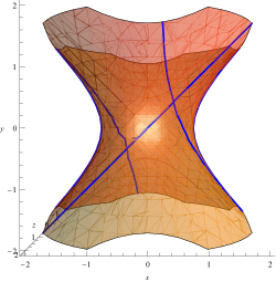
Figure 2: The lines of intersection of $x^{2}-y^{2}+z^{2}=1$ and $x-y=\frac{1-z^{2}}{z}$: $x=y$ and $z=-1$ or $z=1$, and $2z^{2}-2yz=1$. The brane solution corresponds to points on the line $x=y$ in the plane $z=1$, and the point $(0,0,1)$ corresponds to Minkowski space.

Returning to the brane solution, given by the line of points $x=y$ in the plane $z=1$, we note that from $N=1+q\xi$ we may read off $\xi(x,y,z)$ as $N^{-1}=2z(z-y)-1=1-2y$, hence $q\xi=\frac{2x}{1-2x}$. The map between coordinates is ill-defined at $x=\frac{1}{2}$ and as $x\to\pm\infty$ then $q\xi\to-1$. The range $x\in[0,\frac{1}{2})$ corresponds to $\xi\in[0,\infty]$, with $\xi=0$ being Minkowski space. In summary the brane solution corresponds to the points $(x,x,1)$ where $x\in[0,\frac{1}{2})$, which lie on the hyperboloid $x^{2}-y^{2}+z^{2}=1$ representing the coset $\frac{SL(2,\mathbb{R})}{SO(1,1)}$.

Appendix B The reduction of the $4-$dimensional Einstein action to an action in terms of the $3$-metric

In $4$-dimensional space-time the Einstein-Hilbert action can be written as

$$\int d^{4}x\sqrt{-g}L\left(g_{\mu\nu},\partial_{\gamma}g_{\mu\nu}\right)$$ (104)

where $L$ is written as

$$L=R$$ (105)

where $R$ is the Ricci scalar (and we have excluded any cosmological constant and constant of proportionality). Moreover

$$R=q_{\mu}\,^{\nu\lambda\delta}R^{\mu}\,_{\nu\lambda\delta}$$ (106)

with $q_{\mu}\,^{\nu\lambda\delta}=\frac{1}{2}(\delta_{\mu}^{\lambda}g^{\nu\delta}-\delta_{\mu}^{\delta}g^{\nu\lambda})$. We note that

$$\sqrt{-g}L=2\partial_{\gamma}\left[\sqrt{-g}q_{\alpha}\,^{\beta\gamma\delta}\Gamma^{\alpha}_{\beta\delta}\right]+2\sqrt{-g}q_{\alpha}^{\beta\gamma\delta}\Gamma^{\alpha}_{\delta\kappa}\Gamma^{\kappa}_{\beta\gamma}.$$ (107)

We shall ignore the total derivative term in (107) and so the new form of the the Einstein-Hilbert action (which does not contain any terms which contain second derivatives in the metric) is

$$-\int d^{4}x\sqrt{-g}\mathcal{G}$$ (108)

where

$$\mathcal{G}=g^{\mu\nu}\left(\Gamma^{\alpha}_{\mu\beta}\Gamma^{\beta}_{\nu\alpha}-\Gamma^{\alpha}_{\mu\nu}\Gamma^{\beta}_{\alpha\beta}\right).$$ (109)

In order to rewrite $\mathcal{G}$ in terms of metrics on space-like foliations of space-time it is convenient to work in Gaussian co-ordinates. Any space-like hypersurface $S$ in this foliation will be intersected orthogonally by a family of geodesics. The length along these geodesics will give the time. It is then consistent to write the metric in terms of a $3$-metric $\gamma_{ij}$ ($1\leqslant i,j\leqslant 3$) as follows:

$$\left(\begin{array}[]{cccc}1&0&0&0\\ 0&\gamma_{11}&\gamma_{12}&\gamma_{13}\\ 0&\gamma_{21}&\gamma_{22}&\gamma_{23}\\ 0&\gamma_{31}&\gamma_{32}&\gamma_{33}\end{array}\right).$$

In earlier work, considering the vicinity of a space-like singularity, the $\gamma_{ij}$ were taken to be functions of time $t$. In this work we are allowing $\gamma_{ij}$ to be functions of two parameters, time $t$ and space $x$. In both cases $\mathcal{G}$ leads to a similar structure in terms of $\gamma_{ij}$. Explicitly, for the case of two parameters,

$$\mathcal{G}=\frac{1}{4}\left((Tr\left[\gamma^{-1}\partial_{t}\gamma\right])^{2}+(Tr\left[\gamma^{-1}\partial_{x}\gamma\right])^{2}-Tr\left[\gamma^{-1}\partial_{t}\gamma\right]^{2}-Tr\left[\gamma^{-1}\partial_{x}\gamma\right]^{2}\right)$$ (110)

which reduces to the one parameter result when $\gamma_{ij}$ is a function of $t$ only.

References

- [1] P. C. West, “E(11) and M theory,” Class.Quant.Grav. 18 (2001) 4443–4460, arXiv:hep-th/0104081 [hep-th].
- [2] T. Damour, M. Henneaux, and H. Nicolai, “E(10) and a ’small tension expansion’ of M theory,” Phys.Rev.Lett. 89 (2002) 221601, arXiv:hep-th/0207267 [hep-th].
- [3] T. Damour, M. Henneaux, and H. Nicolai, “Cosmological billiards,” Class. Quant. Grav. 20 (2003) R145–R200, arXiv:hep-th/0212256 [hep-th].
- [4] F. Englert and L. Houart, “G+++ invariant formulation of gravity and M theories: Exact BPS solutions,” JHEP 0401 (2004) 002, arXiv:hep-th/0311255 [hep-th].
- [5] L. Houart, A. Kleinschmidt, and J. L. Hornlund, “Some Algebraic Aspects of Half-BPS Bound States in M-Theory,” JHEP 1003 (2010) 022, arXiv:0911.5141 [hep-th].
- [6] P. P. Cook, “Bound States of String Theory and Beyond,” JHEP 1203 (2012) 028, arXiv:1109.6595 [hep-th].
- [7] P. P. Cook, “Exotic E(11) branes as composite gravitational solutions,” Class.Quant.Grav. 26 (2009) 235023, arXiv:0908.0485 [hep-th].
- [8] B. Julia, “GROUP DISINTEGRATIONS,” Conf.Proc. C8006162 (1980) 331–350.
- [9] C. M. Hull, “Duality and the signature of space-time,” JHEP 11 (1998) 017, arXiv:hep-th/9807127 [hep-th].
- [10] A. Keurentjes, “Poincare duality and G+++ algebra’s,” Commun. Math. Phys. 275 (2007) 491–527, arXiv:hep-th/0510212 [hep-th].
- [11] A. Kleinschmidt and P. C. West, “Representations of G+++ and the role of space-time,” JHEP 02 (2004) 033, arXiv:hep-th/0312247 [hep-th].
- [12] W. Siegel, “Superspace duality in low-energy superstrings,” Phys. Rev. D48 (1993) 2826–2837, arXiv:hep-th/9305073 [hep-th].
- [13] C. Hull and B. Zwiebach, “Double Field Theory,” JHEP 09 (2009) 099, arXiv:0904.4664 [hep-th].
- [14] O. Hohm and H. Samtleben, “Exceptional Form of D=11 Supergravity,” Phys. Rev. Lett. 111 (2013) 231601, arXiv:1308.1673 [hep-th].
- [15] M. J. Duff, “Duality Rotations in String Theory,” Nucl. Phys. B335 (1990) 610.
- [16] M. J. Duff and J. X. Lu, “Duality Rotations in Membrane Theory,” Nucl. Phys. B347 (1990) 394–419.
- [17] H. A. Buchdahl, “Reciprocal Static Solutions of the Equations ,” The Quarterly Journal of Mathematics 5 (1954) no. 1, 116–119.
- [18] J. Ehlers, Konstruktionen und Charakterisierung von Losungen der Einsteinschen Gravitationsfeldgleichungen. PhD thesis, Universitat Hamburg, 1957.
- [19] R. P. Geroch, “A Method for generating solutions of Einstein’s equations,” J. Math. Phys. 12 (1971) 918–924.
- [20] R. P. Geroch, “A Method for generating new solutions of Einstein’s equation. 2,” J. Math. Phys. 13 (1972) 394–404.
- [21] E. Cremmer and B. Julia, “The N=8 Supergravity Theory. 1. The Lagrangian,” Phys. Lett. B80 (1978) 48.
- [22] E. Cremmer and B. Julia, “The SO(8) Supergravity,” Nucl. Phys. B159 (1979) 141–212.
- [23] C. W. Misner, “Quantum cosmology. 1.,” Phys. Rev. 186 (1969) 1319–1327.
- [24] C. W. Misner, MINISUPERSPACE, vol. Magic Without Magic: John Archibald Wheeler edited by John R. Klauder, p. 441. W. H. Freeman and Company Ltd, 1972.
- [25] P. P. Cook and M. Fleming, “Gravitational Coset Models,” JHEP 1407 (2014) 115, arXiv:1309.0757 [hep-th].
- [26] A. Borisov and V. Ogievetsky, “Theory of Dynamical Affine and Conformal Symmetries as Gravity Theory,” Theor.Math.Phys. 21 (1975) 1179.
- [27] A. Kleinschmidt, I. Schnakenburg, and P. C. West, “Very extended Kac-Moody algebras and their interpretation at low levels,” Class.Quant.Grav. 21 (2004) 2493–2525, arXiv:hep-th/0309198 [hep-th].
- [28] P. C. West, “The IIA, IIB and eleven-dimensional theories and their common E(11) origin,” Nucl.Phys. B693 (2004) 76–102, arXiv:hep-th/0402140 [hep-th].
- [29] M. Henneaux, D. Persson, and P. Spindel, “Spacelike Singularities and Hidden Symmetries of Gravity,” Living Rev.Rel. 11 (2008) 1, arXiv:0710.1818 [hep-th].
- [30] A. Keurentjes, “E(11): Sign of the times,” Nucl. Phys. B697 (2004) 302–318, arXiv:hep-th/0402090 [hep-th].
- [31] M. J. Duff and K. S. Stelle, “Multimembrane solutions of D = 11 supergravity,” Phys. Lett. B253 (1991) 113–118.
- [32] C. M. Hull and R. R. Khuri, “Branes, times and dualities,” Nucl. Phys. B536 (1998) 219–244, arXiv:hep-th/9808069 [hep-th].
- [33] M. P. Blencowe and M. J. Duff, “Supermembranes and the Signature of Space-time,” Nucl. Phys. B310 (1988) 387–404.
- [34] A. Kleinschmidt and H. Nicolai, “E(10) cosmology,” JHEP 01 (2006) 137, arXiv:hep-th/0511290 [hep-th].
- [35] J. Berkeley, D. S. Berman, and F. J. Rudolph, “Strings and Branes are Waves,” JHEP 06 (2014) 006, arXiv:1403.7198 [hep-th].
- [36] D. S. Berman and F. J. Rudolph, “Strings, Branes and the Self-dual Solutions of Exceptional Field Theory,” JHEP 05 (2015) 130, arXiv:1412.2768 [hep-th].
- [37] D. S. Berman and F. J. Rudolph, “Branes are Waves and Monopoles,” JHEP 05 (2015) 015, arXiv:1409.6314 [hep-th].
- [38] I. Bakhmatov, A. Kleinschmidt, and E. T. Musaev, “Non-geometric branes are DFT monopoles,” JHEP 10 (2016) 076, arXiv:1607.05450 [hep-th].
- [39] C. D. A. Blair, “Doubled strings, negative strings and null waves,” arXiv:1608.06818 [hep-th].