The time evolution of HH 2 from four epochs of HST images

Abstract

We have analyzed four epochs of H$\alpha$ and [S II] HST images of the HH 1/2 outflow (covering a time interval from 1994 to 2014) to determine proper motions and emission line fluxes of the knots of HH 2. We find that our new proper motions agree surprisingly well with the motions measured by Herbig & Jones (1981), although there is partial evidence for a slight deceleration of the motion of the HH 2 knots from 1945 to 2014. We also measure the time-variability of the H$\alpha$ intensities and the [S II]/H$\alpha$ line ratios, and find that knots H and A have the largest intensity variabilities (in $1994\to 2014$). Knot H (which now dominates the HH 2 emission) has strengthened substantially, while keeping an approximately constant [S II]/H$\alpha$ ratio. Knot A has dramatically faded, and at the same time has had a substantial increase in its [S II]/H$\alpha$ ratio. Possible interpretations of these results are discussed.

1 Introduction

The HH 1/2 system is probably the best studied Herbig-Haro flow from a young star (see the review of Raga et al. 2011). This object consists of a central source seen at radio wavelengths (Pravdo et al. 1985; Rodríguez et al. 2000), a bipolar jet/counter jet system (seen in the IR, Noriega-Crespo & Raga 2012), and two “heads” (HH 1 to the NW and HH 2 to the SE) at approximately $1^{\prime}$ from the outflow source. The HH 1/2 outflow axis lies within $\sim 5^{\circ}$ from the plane of the sky (see, e. g., Böhm & Solf 1985).

There are now four epochs of Hubble Space Telescope (HST) images of the HH 1/2 system, covering a $\sim 20$ yr time span. These images were used by Raga et al. (2016a) to measure the proper motions and the time-evolution of the line intensities of HH 1. In the present paper we use the same set of images to study the time-evolution of HH 2.

While HH 1 is a relatively compact collection of knots (with an angular size of $\sim 15^{\prime\prime}$), showing a general organization into a bow-like structure, HH 2 is angularly more extended ($\sim 30^{\prime\prime}$), and has a relatively chaotic condensation structure (see, e.g., Raga et al. 2015b). Because of this, it is more complex to untangle the time-evolution of this object.

In this paper, we calculate the proper motions of the HH 2 condensations. This represents a continuation of the work of Herbig & Jones (1981), Eislöffel et al. (1994) and Bally et al. (2002), who have previously studied the motions of HH 2.

We also calculate the time-evolution of the H$\alpha$ intensities and the [S II]/H$\alpha$ ratios of the HH 2 condensations. This is to some extent an extension of the work of Herbig (1969), who studied the time-evolution of the broad-band emission of of the HH 2 knots, and of the work of Raga et al. (2016b), who compared the angularly integrated emission of HH 2 obtained from HST images and the spectrophotometric observations of Brugel et al. (1981).

The paper is organized as follows. In Section 2 we describe the available set of four epochs of HST images of HH 2. In Section 3, we describe the qualitative time-evolution of the morphology of HH 2. In Section 4, we present the proper motion determinations. In Section 5, we discuss the time evolution of the H$\alpha$ intensity and [S II]/H$\alpha$ line ratios of the HH 2 condensations. Section 6 discusses possible interpretations of the motions and intensity variabilities of the HH 2 knots. Finally, the results are summarized in Section 7.

2 The observations

There are now four epochs of HST H$\alpha$ images (obtained with the F656N filter) and red [S II] images (with the F673N filter) of the HH 1/2 outflow, which we label:

• 1994: the 1994.61 images of Hester et al. (1998),

• 1997: the 1997.58 images of Bally et al. (2002),

• 2007: the 2007.63 images of Hartigan et al. (2011),

• 2014: the 2014.63 images of Raga et al. (2015a, b).

The first three epochs were obtained with the WFPC2 camera, and the fourth epoch with the WFC3. The F656N and F673N filters in of the two cameras are roughly equivalent. A description of the characteristics of these images is given by Raga et al. (2016a), who used them to study the time-evolution of HH 1. In the present paper we use the same images (not corrected for reddening), with the flux calibration and the alignment (between the successive epochs) described by Raga et al. (2016a). All of the images have a $0^{\prime\prime}.1$ per pixel scale.

As discussed by Raga et al. (2015a, 2016a), the H$\alpha$ filters include a contribution of the [N II] 6548 line at a level of $\sim 2$% and a continuum flux at a level of $\sim 1$%  (of the H$\alpha$ flux). The [S II] filters are contaminated by the continuum emission at a level of $\sim 1$% of the [S II] flux. As the initial images have a good signal-to-noise ratio and because additionally our flux measurements are done in decreased angular resolution images (which were convolved with a $1^{\prime\prime}$ wavelet, see section 5), the errors due to photon statistics are small compared to the line and continuum contamination of the filters.

The main contribution to the errors in the line fluxes lies in the flux calibration of the filters. As described by Raga et al. (2016a), the standard continuum calibration of the filters (see, e.g., the WFC3 Instrument Handbook) has been converted into a calibration for the line fluxes using the full width of the filters (see the discussion of O’Dell et al. 2013). This gives an “exact” calibration only for a “box car” filter transmission function, but of course has errors that depend on the exact position within the filter of the emission line for the actual curved filter transmissions. The errors associated with this effect can be estimated by calculating the standard deviation from a box car function of the actual filter transmission curves (given in the WFPC2 and WFC3 Instrument Handbook). From the plotted curves, we obtain standard deviations of $(8.5,3.2)$% (as a percentage of the mean transmission) for the F656N filter and $(6.1,4.8)$% for the F673N filter (the first of the values within the parentheses corresponding to the WFPC2 camera filters and the second one to the WFC3 camera).

We then estimate the errors in the H$\alpha$ and [S II] line fluxes considering the line/continuum contamination and the flux calibration errors. In this way we obtain estimates of $(9,4)$% for the line flux errors of the F656N frames (as percentages of the H$\alpha$ fluxes) and $(6,5)$% for the F673N filters (as percentages of the [S II] line fluxes), with the first and second values in the parentheses corresponding to the WFPC2 and WFC3 cameras, respectively.

The four epochs of H$\alpha$ images are shown in Figure 1 (with a field that includes all of the HH 2 emission) and in Figure 2 (a smaller field including the brighter knots H and A), and the four [S II] images are shown in Figures 3 and 4. Figures 5 and 6 show the four H$\alpha$ and [S II] images (respectively), convolved with a “Mexican hat” wavelet with a central peak of $1^{\prime\prime}$ radius. These convolved images have a resolution comparable to ground-based images.

We note a particular difficulty that is found when measuring the positions of the knots of HH 2. The images are scaled, rotated and aligned using the positions of the Cohen-Schwartz star (Cohen & Schwartz 1979) and “star no. 4” of Ström et al. (1985). The positions of these two stars (the CS star along the outflow axis and star no. 4 approximately $1^{\prime}$ to the E of the CS star) are closer by a factor of $\sim 3$ to HH 1 than to HH 2. Because of this, the error in the positions of the HH 2 knots (dominated by the effect of the rotation of the frames rather than by the scaling) are considerably larger than the errors for the positions of HH 1 (measured by Raga et al. 2016a). This problem in measuring the positions of the HH 2 knots in CCD frames that only include these two stars was already noted in the first attempt to carry out astrographic measurements of HH objects with CCD frames (Raga et al. 1990).

We find that the errors in the centering/scaling/rotation of the four epochs of images of HH 2 are dominated by offsets perpendicular to the outflow axis (with a PA=325^∘ direction see Bally et al. 2002), with values of $\sim 0^{\prime\prime}.2$. These errors result in systematic shifts (between the successive epochs) of all of the HH 2 knots in the direction perpendicular to the outflow axis. One could in principle apply a small correction to the rotations of the successive frames in order to minimize these systematic offsets, but we feel that it is better not to apply such a correction.

3 Morphological changes of HH 2

In Figure 1, we show the H$\alpha$ emission of HH 2 in the four epochs. In the 1994 frame (top left frame), we show the identifications of the emitting knots of Herbig & Jones (1981) and Eislöffel et al. (1994). It is clear that while the knots in the periphery of HH 2 (knots T, E, L and D) have a similar morphology in the four frames, the knots in the brighter, central region of HH 2 (knots G, H and A) have rather dramatic changes. Knot K is a peripheral knot, and it shows considerable intensity changes while preserving its general morphology.

The time-evolution of part of the central region of HH 2 (i.e., the region shown with a white box in the bottom right frame of Figure 1) is shown in Figure 2. In this figure, we see that condensation H has dramatic morphological changes (as well as a strong brightening) and condensation A an also dramatic fading during the period covered by the four HST frames.

The four [S II] frames are shown in Figure 3. We find a behaviour similar to the H$\alpha$ images, with the knots on the periphery of HH 2 preserving their morphological characteristics, and with large variabilities in the central knots. This effect is clearly seen in Figure 4, which shows the [S II] emission of the central region of HH 2.

4 The proper motions

Given the large morphological changes in the HH 2 knots at subarcsecond scales (see Figures 2 and 4), in order to obtain proper motions, following Raga et al. (2016a) we first convolve the images with a “Mexican hat” wavelet with a central peak of radius $\sigma=1^{\prime\prime}$ (see equation 1 of Raga et al. 2016a). The resulting H$\alpha$ (see Figure 5) and [S II] (see Figure 6) convolved images show well defined peaks for the condensations L, E, G, H, I, T, A and D. In the convolved images, Knot K has two peaks which we call K1 (the E peak) and K2 (the W peak, see Figures 5 and 6).

We then carry out paraboloidal fits to $3\times 3$ pixel regions centered on these peaks and measure offsets with respect to the knot positions in the 1994 frame. We adopt a PA=145^∘ position angle for the outflow axis of HH 2 (with a direction opposite to the PA=325^∘ direction of the HH 1 jet obtained by Bally et al. 2002) and calculate the offsets parallel ($\Delta x$) and perpendicular ($\Delta y$) to the outflow axis (with positive values of $\Delta y$ directed to the W of the outflow axis) between the knots in the successive frames and their positions in the 1994 frame. The offsets obtained in the H$\alpha$ and in the [S II] frames are shown in Figures 7 and 8.

In Figures 7 and 8 we see that:

• the H$\alpha$ and [S II] offsets are consistent for all knots, except for the offsets along the outflow axis ($\Delta x$) of knot I and the $\Delta y$ offsets of knot L,

• the largest offsets along the outflow axis ($\Delta x$) are seen for knot I (with inconsistent H$\alpha$ and [S II] offsets), and are therefore somewhat suspect,

• the central knots of HH 2 (knots G, H and A) have $\Delta x\sim 5\Delta y$ and the peripheral knots (knots E, K1, K2, T and D) have $\Delta x\sim\Delta y$,

• a systematic “down/up” pattern (with an amplitude of $\sim 0^{\prime\prime}.2$) is seen in the successive $\Delta y$ values, which probably results from the frame centering problems discussed in Section 2.

Table 1 shows the velocities parallel ($v_{x}$) and perpendicular ($v_{y}$) to the outflow axis obtained from linear, least squares fits to the H$\alpha$ and [S II] offsets and assuming a distance of 414 pc to HH 2 (Menten et al. 2007). The $\epsilon(v_{x})$ and $\epsilon(v_{y})$ errors computed from the fits are also given. The linear fits are plotted for all of the knots in Figures 7 and 8, showing that the scatter of the measured points is large enough that a fit with a higher order polynomial (as would be needed to estimate an acceleration/deceleration for the knots) would be meaningless.

In Table 1, we also give the proper motion velocity $v_{t}=\sqrt{v_{x}^{2}+v_{y}^{2}}$ and its associated error $\epsilon(v_{t})$, as well as the proper motion velocities $v_{HJ}$ obtained by Herbig & Jones (1981) for some of the knots. The values of $v_{HJ}$ were obtained from the analysis of red photographic plates obtained from 1945 to 1980 of Herbig & Jones (1981), which we have now corrected to a distance of 414 pc to HH 2.

The consistency between our values of $v_{t}$ and the corresponding $v_{HJ}$ values of Herbig & Jones (1981) is quite remarkable:

• for knots E, G, H and D we obtain slightly lower proper motion velocities than the $v_{HJ}$ values of Herbig & Jones (1981), though the difference in velocities is probably only significant for knots G and D,

• for knot A, we obtain a higher proper motion velocity than its $v_{HJ}$ value, but this is probably not a significant result given the problems found by Herbig & Jones (1981) for determining the proper motion of this condensation (for which they did not give an estimated error),

• for knot I (with inconsistent H$\alpha$ and [S II] proper motions, see above), we see that our H$\alpha$ proper motion velocity is somewhat higher than $v_{HJ}$ and that our [S II] velocity is substantially lower.

Therefore, what can be said is that for some of the knots (knots E, G, H and D) we might be seeing a slight slowing down between the $1945\to 1980$ period (analyzed by Herbig & Jones 1981) and the $1994\to 2014$ period that we are now analyzing, but that this effect is rather marginal.

We should also mention that it is not possible to compare our results with the proper motions obtained by Eislöffel et al. (1994) and by Bally et al. (2002), because these authors calculated offsets for small angular scale structures within the larger scale knots of Herbig & Jones (1981). It is not possible to recognize these smaller scale structures in the more recent HST frames that we are analyzing, as a substantial morphological evolution has occurred (see the discussion of section 3).

5 The H$\alpha$ fluxes and the [S II]/H$\alpha$ line ratios

From paraboloidal fits to the peaks of the convolutions of the H$\alpha$ and [S II] images with a $1^{\prime\prime}$ wavelet (see the discussion of Section 4 and Figures 5 and 6), we obtain a peak intensity $I_{p}$ for each knot. We can then calculate the flux associated with the peak of the structure as $F_{p}=\pi\sigma^{2}I_{p}$ (where $\sigma=1^{\prime\prime}$ is the radius of the central peak of the wavelet, see Section 4).

The H$\alpha$ fluxes and the [S II]/H$\alpha$ ratios for the HH 2 knots in the four epochs are shown in Figures 9 and 10. In these Figures, we show the errors for the H$\alpha$ fluxes and for the [S II]/H$\alpha$ line ratios corresponding to the errors discussed in section 2.

Several interesting features can be seen in these plots:

• knot H (which dominates the emission of HH 2) has an H$\alpha$ flux that has grown by a factor of $\approx 2.9$ between 1994 and 2014, while keeping a [S II]/H$\alpha$ ratio with variations of only $\sim 20$%,

• knot A shows a decrease by a factor of $\approx 14$ in its H$\alpha$ flux, and an increase in its [S II]/H$\alpha$ ratio from $\approx 0.2$ (in 1994) to $\approx 0.9$ (in 2014),

• knot D shows a decrease by a factor of $\approx 1.7$ in H$\alpha$, and an approximately constant [S II]/H$\alpha$ ratio,

• knot K1 shows an increase by a factor of $\approx 1.6$ in H$\alpha$, and an increase by a factor of $\approx 1.3$ in the [S II]/H$\alpha$ ratio and knot K2 shows an H$\alpha$ increase of $\approx 2.4$ and a [S II]/H$\alpha$ increase of $\approx 1.8$,

• knot I shows an almost constant H$\alpha$ flux, and a [S II]/H$\alpha$ ratio with relatively strong variations. This latter feature again might be a result of the inconsistent results that we obtain in the H$\alpha$ and [S II] structures for this knot (see Section 3),

• the remaining knots (L, E and T) show H$\alpha$ fluxes and [S II]/H$\alpha$ ratios with only small variations in the period covered by the observations.

The strongest H$\alpha$ variabilities are seen in knots H and A. The implications of these two behaviours will be discussed in the following section.

6 Interpretation

6.1 The dispersion of the proper motions

Raga et al. (1997) considered the proper motions of a system of condensations that form part of a single, bow-shock like structure of velocity $v_{bs}$ travelling into an environment which is moving away from the source at a uniform velocity $v_{a}$ ($<v_{bs}$). They show that the total range of possible proper motion velocities along ($\Delta v_{x}$) and across ($\Delta v_{y}$) the outflow axis are both equal to $v_{bs}-v_{a}$. This result is somewhat counter-intuitive, but is indeed the result obtained for a curved bow shock covering all possible angles between the shock surface and the outflow axis (similar results, but for the radial velocities, were obtained previously by Hartigan et al. 1997). However, because one has a finite (and rather small) number of condensations, the actual values of $\Delta v_{x}$ and $\Delta v_{y}$ can be somewhat smaller than $v_{bs}-v_{a}$. Also, the proper motions along the outflow axis have $v_{a}$ (the outflowing velocity of the pre-bow shock environment) as a minimum possible value.

Considering the H$\alpha$ proper motion velocities of Table 1 (and not considering knot I, which has inconsistent H$\alpha$ and [S II] proper motions), we obtain $\Delta v_{x}=167$ and $\Delta v_{y}=94$ km s^-1. Also, the lowest axial proper motion leads to a $v_{a}\sim 39$ km s^-1 value for a possible outflowing motion of the pre-bow shock environment. These values indicate that a single bow shock interpretation of HH 2 implies that the object is moving at a velocity of $\sim 170$ km s^-1 into a low velocity medium, with a $v_{a}\sim 40$ km s^-1 maximum possible velocity.

However, the factor of $\sim 1.8$ discrepancy between $\Delta v_{x}$ and $\Delta v_{y}$ indicates that the simple, post-bow shock emission model of Raga et al. (1997) is probably incorrect (as it predicts that $\Delta v_{x}\sim\Delta v_{y}$). This could be due to:

• the condensations of HH 2 do not correspond to a single bow shock flow travelling into an outflowing environment with a single velocity $v_{a}$ (which would not be surprising given the complex morphology of the object!),

• the condensations could trace a single bow shock, but the emission could come not from the immediate post-shock gas but from material which has been substantially mixed with the jet material (which would have the effect of re-aligning the velocity of the emitting gas to a direction closer to the outflow axis).

6.2 Condensations H and A

These are the condensations with the strongest H$\alpha$ variabilities, and follow trends of increasing (knot H) and decreasing (knot A) intensities, that can be traced back to at least 1954, when knot A was the dominant knot of HH 2 (see Herbig 1969). Nowadays, condensation H dominates the emission from HH 2, and participates in the long-term trend (from $\sim 1980$ onwards) of increasing intensities and approximately constant line ratios noted by Raga et al. (2016b) for HH 2.

As discussed by Raga et al. (2016b), an emitting knot with an increasing luminosity and at the same time almost constant line ratios could correspond to a high density jet travelling into a region of increasing environmental density (but with smaller values than the jet density). If this scenario is applicable to HH 2H, the condensation should have an almost constant velocity (necessary for obtaining the time-independent line ratios), with a small velocity decrease as a function of time (resulting from the increasing environmental density). As discussed in Section 4, a small decrease in the proper motion of condensation H might be seen in the comparison between our measurements and the ones of Herbig & Jones (1981).

From 1994 to 2014, condensation A has had a dramatic decrease in its H$\alpha$ intensity (by a factor of $\sim 14$), accompanied by a strong increase in its [S II]/H$\alpha$ ratio. During this period, this ratio has changed from a value of $\sim 0.2$ to $\sim 0.9$ . Given the fact that Herbig & Jones (1981) judged their proper motion of condensation A to be quite uncertain, it is not clear whether this knot has decelerated, but if we take their proper motion velocity at face value, it appears that the condensation has mildly accelerated (see Section 4 and Table 1). This combination of decreasing H$\alpha$ intensity, increasing [S II]/H$\alpha$ ratio and basically constant (and possibly slightly growing) velocity cannot be explained with a model of the emission coming from an angularly unresolved cooling region behind a stationary shock (for the predictions from such models see, e.g., Hartigan et al. 1987). However, if knot A had slowed down in a considerable way (which could be possible given the lack of an error estimation in the knot A proper motion of Herbig & Jones 1981), the behaviour of the H$\alpha$ and [S II] emission of knot A might indeed be consistent with plane-parallel shock models.

7 Summary

We have used four epochs of H$\alpha$ and [S II] HST images (covering a time baseline of approximately 20 years) to carry out measurements of the proper motions of the condensations of HH 2. Because the subarcsecond structure has relatively large morphological changes (see Section 3 and Figures 1-4), it is necessary to reduce the resolution of the image in order to have intensity peaks that can clearly be identified in the successive epochs. We have done this by convolving the images with a wavelet function having a central peak of radius $\sigma=1^{\prime\prime}$ (see Section 4 and Figures 5-6).

In these convolved images, we identify 10 knots which can be clearly seen in all of the four epochs, and for these knots we calculate the proper motions (deduced from fits to the positions of the peaks in the four epochs, see Section 4, Figures 7-8 and Table 1). We find that all of the knots have motions consistent with a constant velocity (i.e., an acceleration or deceleration is not seen in a clear way for any of the knots). Also, we see that the H$\alpha$ and [S II] proper motions are consistent for all of the knots except knot I.

We can compare our proper motion velocities with the ones carried out by Herbig & Jones (1981), who measured the velocities of knots E, G, H, I, A, D and C on photographic plates covering the period from 1945 to 1980. For knots E, G, H and D, we find slightly lower proper motion velocities than the ones of Herbig & Jones (1981), and a somewhat higher velocity for knot A (see Table 1). It is not clear that this latter effect is significant, because Herbig & Jones (1981) discuss in detail that their proper motions for knot A are strongly affected by large morphological changes of this knot. For knot I, we find that our H$\alpha$ proper motion is somewhat higher and our [S II] proper motion is substantially lower than the proper motion of Herbig & Jones (1981). For knot C (which was measured by Herbig & Jones 1981) we have been unable to obtain a proper motion because of its present day faintness (in H$\alpha$) and its complex morphological evolution.

The conclusion from this comparison between our proper motions and the ones of Herbig & Jones (1981) is that we might be observing a deceleration of the motion of the HH 2 knots, but that this is a small and somewhat uncertain effect. Taken at face value, this effect could be interpreted either in terms of dense clumps which are being braked by the interaction with the surrounding environment, or as the (broken-up) head of a jet travelling into an ambient medium of increasing density (as a function of distance from the outflow source).

We have also measured the H$\alpha$ intensities and [S II]/H$\alpha$ line ratios (of the knots seen in the convolved images shown in Figures 5 and 6) in the four observed epochs. We find that during 1994-2014 many of the observed knots have small variations in both H$\alpha$ and [S II]/H$\alpha$ (see Figures 10-11). The knots with the largest H$\alpha$ variability are:

• knot H: which has an H$\alpha$ increase by a factor of $\approx 2.4$ and an approximately constant [S II]/H$\alpha$ ratio,

• knot A: which has an H$\alpha$ decrease by a factor of $\approx 14$ and an increase by a factor of $\approx 4$ in its [S II]/H$\alpha$ ratio.

As pointed out by Raga et al. (2016b), who studied the angularly integrated emission of HH 2, the behaviour of knot H could be interpreted as a shock with a time-independent shock velocity travelling into an environment of increasing density. The behaviour of knot A, however, defies an interpretation in terms of a steady shock model.

Table 1: HH 2 proper motions

knot	$v_{x}$a	$\epsilon(v_{x})$a	$v_{y}$a	$\epsilon(v_{y})$a	$v_{t}$a	$\epsilon(v_{t})$a	$v_{HJ}$a	$\epsilon(v_{HJ})$a
L	46.4	4.4	-4.7	20.1	46.7	7.7
	40.3	4.3	47.3	16.6	62.1	14.9
E	27.5	7.1	-47.4	21.7	54.9	20.8	55	20
	30.0	4.8	-41.1	20.8	50.9	19.0
K1	45.6	2.9	-45.8	17.9	64.6	15.3
	49.2	4.5	-49.0	18.1	69.5	15.7
K2	45.6	8.4	-41.1	21.1	61.4	18.7
	44.5	4.3	-45.9	15.4	63.9	13.5
G	97.3	6.9	16.7	20.3	98.7	10.8	138	8
	90.3	5.8	18.0	20.1	92.1	10.6
H	206.6	5.6	-46.5	18.1	211.8	10.1	217	12
	183.5	7.6	-53.9	17.8	191.2	12.0
I	234.9	6.2	-8.9	30.1	235.1	8.5	214	40
	62.3	12.3	5.6	24.5	62.5	14.3
A	144.1	4.9	28.6	15.1	146.9	8.2	138	$\ldots$b
	175.5	10.5	42.8	17.9	180.6	13.5
T	66.0	4.2	-40.9	19.6	77.6	14.7
	65.7	3.9	-42.2	18.8	78.1	14.3
D	39.3	4.7	-12.5	19.2	41.2	11.5	77	20
	32.6	6.0	-6.1	18.9	33.1	10.0

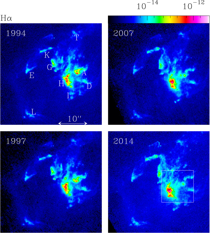
Figure 1: The four available epochs of HST H$\alpha$ frames showing a region including all of the detected HH 2 emission. The four frames are labeled with the year in which the observations were made, and the angular scale is given in the top left frame. The frames are oriented with N on top and E to the left. The emission is shown (in erg s^-1 cm^-2 arcsec^-2) with the logarithmic colour scale given by the top right bar. In the top left frame, the knot identifications are given, following Herbig & Jones (1981). In the bottom right frame, the box shows the region which is covered in the images shown in Figure 2.

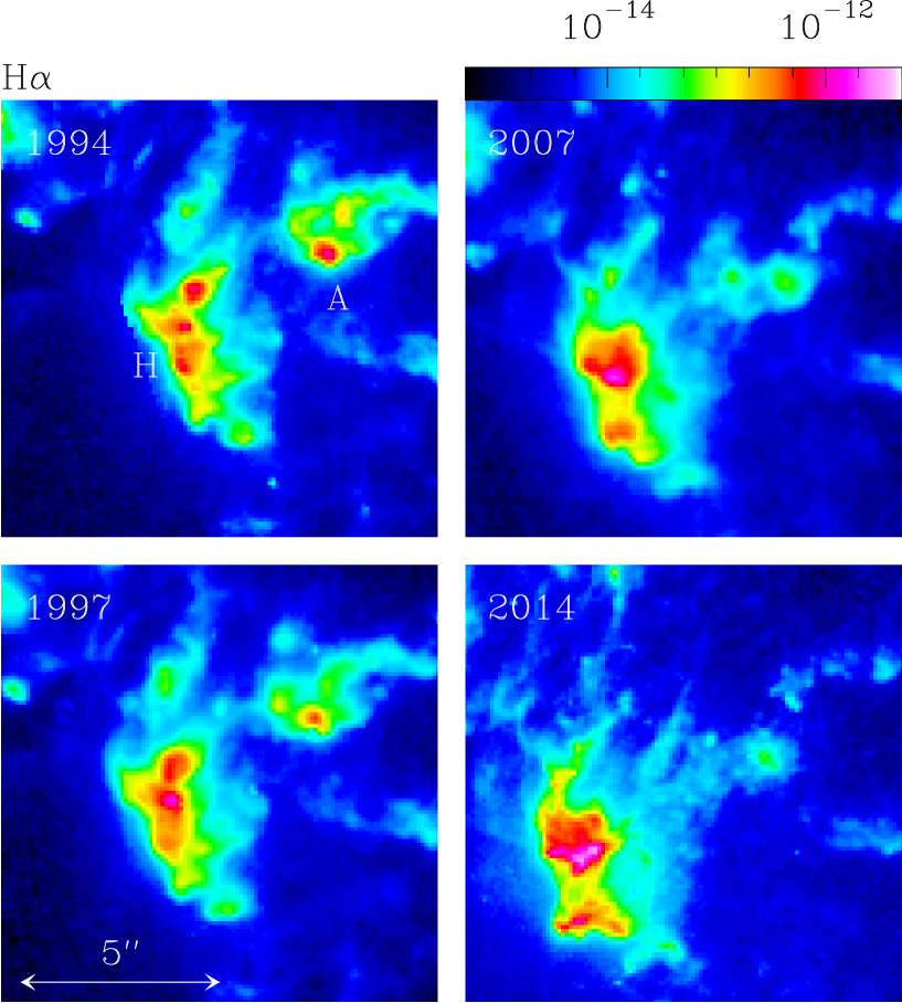
Figure 2: This figure shows the H$\alpha$ emission of the central region of HH 2 (defined by the box in the bottom right frame of Figure 1) in the four epochs of HST images.

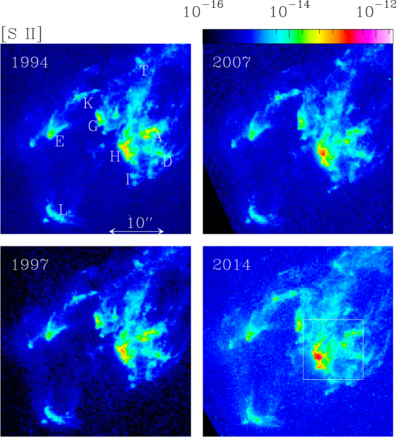
Figure 3: The four available epochs of HST [S II] frames showing a region including all of the detected HH 2 emission. This figure has the same characteristics as Figure 1 (which shows the corresponding H$\alpha$ frames).

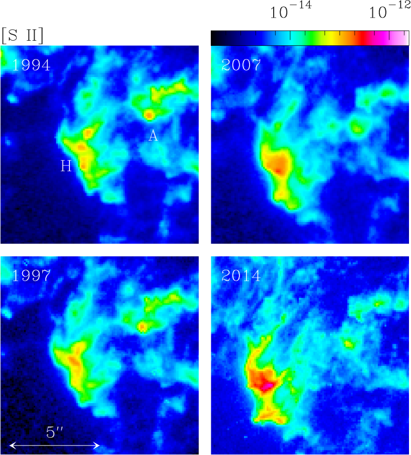
Figure 4: This figure shows the [S II] emission of the central region of HH 2 (defined by the box in the bottom right frame of Figure 3) in the four epochs of HST images.

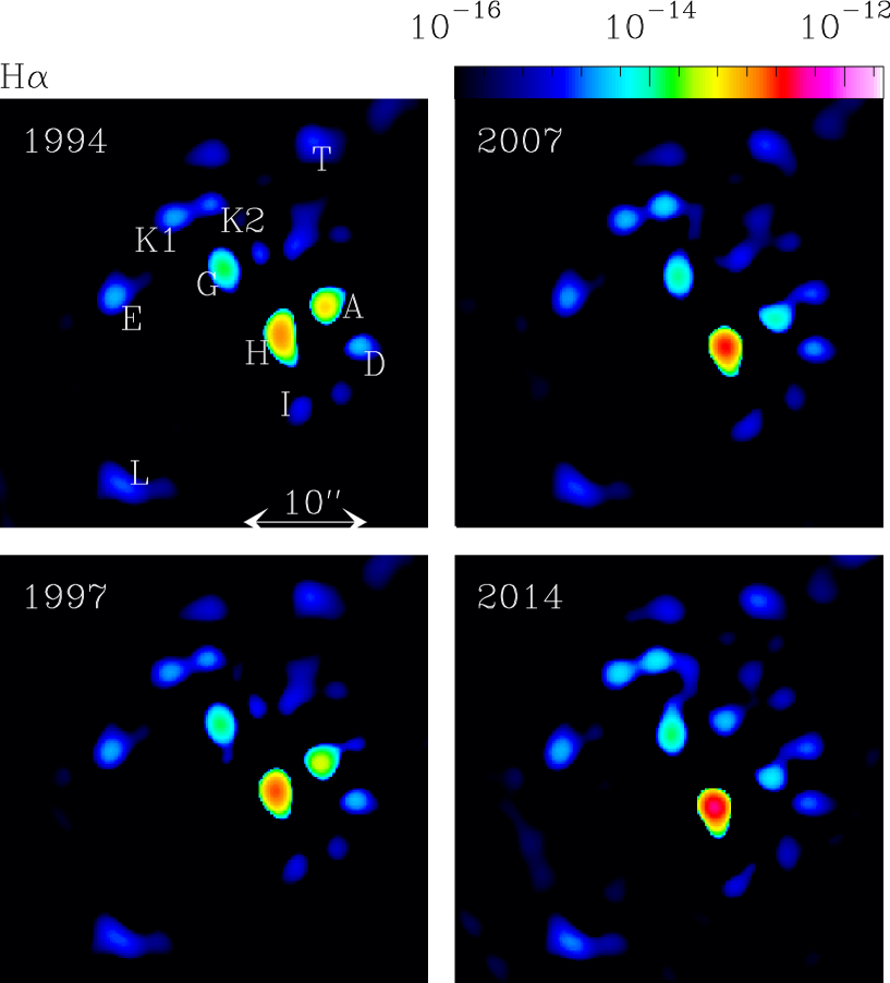
Figure 5: Convolutions of the H$\alpha$ images with a $\sigma=1^{\prime\prime}$ radius “Mexican hat” wavelet. The organization of this figure is the same as the one of Figure 1 (which shows the original H$\alpha$ frames).

Figure 6: Convolutions of the [S II] images with a $\sigma=1^{\prime\prime}$ radius “Mexican hat” wavelet. The organization of this figure is the same as the one of Figure 3 (which shows the original [S II] frames).

Figure 7: Offsets $\Delta x$ (left column, along the outflow axis) and $\Delta y$ (right column, across the outflow axis, with positive values directed to the W) from the 1994 positions as a function of time for knots L, E, K1, K2 and G. The H$\alpha$ offsets are shown with filled circles (and linear fits to the offsets with solid lines) and the [S II] offsets with open circle (and linear fits with dashed lines).

Figure 8: Offsets $\Delta x$ (left column, along the outflow axis) and $\Delta y$ (right column, across the outflow axis, with positive values directed to the W) from the 1994 positions as a function of time for knots H, I, A, T and D. The H$\alpha$ offsets are shown with filled circles (and linear fits to the offsets with solid lines) and the [S II] offsets with open circle (and linear fits with dashed lines).

Figure 9: H$\alpha$ fluxes (left column, in erg s^-1 cm^-2) and [S II]/H$\alpha$ ratios (right column) as a function of time for knots L, E, K1, K2 and G.

Figure 10: H$\alpha$ fluxes (left column, in erg s^-1 cm^-2) and [S II]/H$\alpha$ ratios (right column) as a function of time for knots H, I, A, T and D.

References

- Ballyet al. (2002) Bally, J., Heathcote, S., Reipurth, B., Morse, J., Hartigan, P., & Schwartz, R. D. 2002, AJ, 123, 2627
- Böm & Solf (1985) Böhm, K. H., & Solf, J. 1985, ApJ, 294, 533
- Brugelet al. (1981) Brugel, E. W., Böhm, K. H., & Mannery, E. 1981, ApJS, 47, 117
- auth (year) Cohen, M., & Schwartz, R. D. 1979, ApJ, 233, L77
- auth (year) Eislöffel, J., Mundt, R., & Böhm, K. H. 1994, AJ, 108, 1042
- auth (year) Hartigan, P., Frank, A., Foster, J. M., et al. 2011, ApJ, 736, 29
- auth (year) Hartigan, P., Raymond, J., & Hartmann, L. W. 1987, ApJ, 316, 323
- auth (year) Herbig, G. H. 1969, Comm. of the Konkoly Obs., No. 65 (Vol VI, 1), p. 75
- author (year) Herbig, G. H., & Jones, B. F. 1981, AJ, 86, 1232
- author (year) Hester, J. J., Stapelfeldt, K. R., & Scowen, P. A. 1998, AJ, 116, 372
- author (year) Menten, K. M., Reid, M. J., Forbrich, J., & Brunthaler, A. 2007, A&A, 474, 515
- author (year) Noriega-Crespo, A., & Raga, A. C. 2012, ApJ, 750, 101
- O’Dellet al. (2013) O’Dell, C. R., Ferland, G. J., Henney, W. J., Peimbert, M. 2013, AJ, 145, 92
- author (year) Pravdo, S. H., Rodríguez, L. F., Curiel, S., Cantó, J., Torrelles, J. M., Becker, R. H., & Sellgren, K. 1985, ApJ, 293, L35
- author (year) Raga, A. C., Reipurth, B., Esquivel, A., & Bally, J. 2016a, AJ, 151, 113
- author (year) Raga, A. C., Reipurth, B., Castellanos-Ramírez, A., & Bally, J. 2016b, RMxAA, in press
- author (year) Raga, A. C., Reipurth, B., Castellanos-Ramírez, A., Chiang, H.-F., & Bally, J. 2015a, ApJ, 798, L1
- author (year) Raga, A. C., Reipurth, B., Castellanos-Ramírez, A., Chiang, H.-F., & Bally, J. 2015b, AJ, 150, 105
- author (year) Raga, A. C., Reipurth, B., Cantó, J., Sierra-Flores, M. M., & Guzmán, M. V. 2011, RMxAA, 47, 425
- author (year) Raga, A. C., Cantó, J., Curiel, S., Noriega-Crespo, A., & Raymond, J. C. 1997, RMxAA, 33, 157
- author (year) Raga, A. C., Barnes, P. J., & Mateo, M. 1990, AJ, 99, 1912
- author (year) Rodríguez, L. F., Delgado-Arellano, V. G., Gómez, Y., et al. 2000, AJ, 119, 882
- author (year) Strom, S. E., Strom, K. M., Grasdalen, G. L. et al. 1985, AJ, 90, 2281