Static configurations and evolution of higher dimensional brane-dilaton black hole system

Abstract

Static configurations and a dynamical evolution of the system composed of a higher-dimensional spherically symmetric dilaton black hole and the Dirac-Goto-Nambu brane were investigated. The studies were conducted for three values of the dilaton coupling constant, describing the uncoupled case, the low-energy limit of the string theory and dimensionally reduced Klein-Kaluza theories. When the black hole is nonextremal, two types of static configurations are observed, a brane which intersects the black hole horizon and a brane not having any common points with the accompanying black hole. As the number of spacetime dimensions increases, the brane bend in the vicinity of the black hole disappears closer to its horizon. Dynamical evolution of the system results in an expulsion of the black hole from the brane. It proceeds faster for bigger values of the bulk spacetime dimension and thicker branes. The value of the dilatonic coupling constant does not influence neither the static configurations nor the dynamical behavior of the examined nonextremal system. In the extremal dilaton black hole case one obtains expulsion of the brane which is independent on the spacetime dimensionality and the value of the coupling constant. Dynamical studies of the configurations in the extremal case reveal that the course of evolution of the system is similar to the nonextremal one, except for a slightly earlier expulsion of the black hole from the brane.

1 Introduction

A resurgence of studies of higher-dimensional black holes, black branes and their mutual interactions has been observed recently. These subjects are valid in several different areas of modern theoretical physics. Contemporary candidates of quantum gravity such as the string/M-theory predict that our universe can be described as a brane embedded in a higher-dimensional spacetime. This idea was incorporated in the so-called brane-world models which are composed of a higher-dimensional bulk and a lower-dimensional embedded brane. The first brane-world models were built with a tensionless brane and compactified flat extra dimensions ark98 ; ark99 . Later on, they were extended to the case of a non-zero tension brane and a warped (negatively curved) spacetime ran1 ; ran2 . The Standard Model particles are confined to the brane, while gravity can penetrate the other additional dimensions. In such theories interactions between the brane and black holes were intensively investigated tan11 . Especially, much attention was paid to the problem of higher-dimensional black holes/black objects crossing the brane and the expulsion problem for such systems. In fro06 a toy model for studying a process of merging within the brane-black hole system and a topology change was considered. The higher-dimensional generalizations both in classical general relativity and in certain strongly coupled gauge theories were presented in kol05 ; kol06 ; mat06 ; mat07 . Axisymmetric higher-dimensional systems consisting of stationary test branes interacting with Myers-Perry bulk black holes were examined for arbitrary brane and bulk dimensions czi13 .

One of the predictions of the theories with large extra dimensions is the conjecture that mini black holes with masses of $1$ TeV can be in principle observed in LHC lhc ; lhc1 . Namely, when two particles on the brane collide at the center of mass energy larger than $1$ TeV, the system collapses and the formation of mini black hole begins. With the passage of time the black hole starts to emit Hawking radiation into lower dimensional fields localized on the brane and partly into the higher-dimensional mode, i.e., into the bulk.

The early stages of the evolution of our Universe are also the arenas where primordial black holes and domain walls could have been born. Cosmological density perturbations may have collapsed and led to the formation of small black holes. Next, when the Universe underwent several cooling processes series of phase transitions might occurred leading to the domain wall and other cosmological defects formation vil . In principle, the interaction of black holes with branes (domain walls) should be taken into account when discussing the aforementioned period of the Universe evolution.

In the past few decades, the interactions between black holes and domain walls have been an object of serious studies, both analytical and numerical. A Nambu-Goto membrane in the Reissner-Nordström-de Sitter spacetime was studied in hig00 , while the gravitational system of the Schwarzschild static black hole and a thick domain wall was examined in mor00 ; mor03 . The domain walls were simulated by a scalar field with an adequate potential like $\phi^{4}$ or the sine-Gordon ones. The dilaton black hole-domain wall system was elaborated in rog01 ; mod03 . Among all, it was shown that in the extremal case the expulsion of the scalar field connected with a domain wall took place. In mod04 it was revealed that there was a parameter depending on the black hole mass and the width of a domain wall, which turned out to be an upper limit for the expulsion process. The thick domain wall problem in the anti-de Sitter spacetime was treated in mod06 , while the cosmological brane-black hole system in rog04 . By using the C-metric construction the line element describing an infinitely thin brane intersected by a cosmological black hole was derived.

In fla05 the black hole whose size was small when compared to the extra dimensions was considered (the tension of the brane was negligible). The simulation was conducted by looking for the dynamical evolution of the brane in the fixed background of the black hole. Further studies of the interaction of a black hole with a scalar field domain wall confirm the previously drawn conclusions fla06a . The evolution of the system was also analyzed during the separation process. In fla06b the problem of the influence of the brane tension on the escaping black hole was elaborated. The new challenge was to find if the brane tension might prevent the black hole from escaping for a small recoil velocity. The numerical studies of the interaction of black holes with the field theoretical domain wall, i.e., described by an axion-like field theory with an approximate $U(1)$-gauge symmetry, exploring the topology changing process of a brane perforation was conducted in fla07 . It was revealed that the perforation process depends on the collision velocity and there was a critical value of velocity which suppressed the domain wall perforation.

In cha00 ; sto05 the studies of the domain walls perforation by black holes envisaged that the mechanism is more or less relevant to the cosmological domain wall case. On the other hand, the curvature corrections to the static axisymmetric membrane evolution in the spherically symmetric spacetime of an arbitrary dimensional black hole, were given in czi09 . The problem of a thick brane-black hole system was explored in a series of papers, where perturbative and non-perturbative solutions including the case of a two-brane were studied czi09 ; czi10 ; czi11 . The last moments of a mini black hole escaping from a brane were examined in bal11 . Among all, it was shown that the world sheet becomes isotropic at the reconnection point. It turns out that the higher dimension we examine, the faster the brane becomes isotropic.

A collision of a point particle with an infinitely thin planar domain wall interacting within the linearized gravity in the Minkowski spacetime of an arbitrary dimension was analyzed in gal14 . The energy momentum balance in this system was found in gal14a .

The motivation standing behind our studies is the fact that the classical black hole solutions of Einstein-Maxwell gravity in four or higher dimensions have quite new features when the underlying theory is modified by the introduction of the low-energy string corrections. The key property of the aforementioned correction in the action is connected with the nontrivial coupling of the dilaton field (as well as the other ones like, e.g., axions) with the field strength of the gauge field or gauge fields. There are some models which admit $n$-gauge fields.

In our paper we shall consider static configurations and a dynamical evolution of the higher dimensional spherically symmetric black hole and the Dirac-Goto-Nambu brane (a brane-dilaton black hole (BDBH) system), paying attention to the new features of the system in question. The dilaton black hole was briefly described in section 2 to establish the notations for the bulk spacetime. The studied brane embedded in the black hole spacetime was codimension-one. The theoretical frameworks of the above-mentioned static and dynamical setups, along with computational details and results were presented in sections 3 and 4, respectively. The summary of our findings was presented in section 5.

2 Bulk spacetime containing a higher-dimensional dilaton black hole

The considered black hole was a $d$-dimensional dilaton black hole, whose metric in $\left(t,r,\theta_{i}\right)$ coordinates, where $i=1,...,d-2$, is given by gib88

$$ds^{2} = -\Bigg{[}1-\bigg{(}\frac{r_{+}}{r}\bigg{)}^{d-3}\Bigg{]}\Bigg{[}1-\bigg{(}\frac{r_{-}}{r}\bigg{)}^{d-3}\Bigg{]}^{1-\gamma(d-3)}dt^{2}+$$ (1)

$$+\Bigg{[}1-\bigg{(}\frac{r_{+}}{r}\bigg{)}^{d-3}\Bigg{]}^{-1}\Bigg{[}1-\bigg{(}\frac{r_{-}}{r}\bigg{)}^{d-3}\Bigg{]}^{\gamma-1}dr^{2}+r^{2}\Bigg{[}1-\bigg{(}\frac{r_{-}}{r}\bigg{)}^{d-3}\Bigg{]}^{\gamma}d\Omega_{d-2}^{2},$$

where $r_{+}$ and $r_{-}$ are the radii of two horizons, the outer and inner ones, $r_{+}>r_{-}$. The case when $r_{+}=r_{-}$ is reserved for the extremal higher-dimensional dilaton black hole. $\Omega_{d-2}^{2}$ is the line element of the $d-2$-dimensional unit sphere with coordinates $\theta_{i}$, $i=1,...,d-2$, defined on it by the relations $d\Omega_{i+1}^{2}=d\theta_{i+1}^{2}+\sin^{2}\theta_{i+1}d\Omega_{i}^{2}$. $\gamma$ is an auxiliary constant related to the dilaton coupling constant $\alpha$ and the dimension of the considered spacetime $d$ by the following relation:

$$\gamma=\frac{2\alpha^{2}(d-2)}{(d-3)\left[2(d-3)+\alpha^{2}(d-2)\right]}.$$ (2)

For the brevity, two functions $f_{1}=1-\Big{(}\frac{r_{+}}{r}\Big{)}^{d-3}$ and $f_{2}=1-\Big{(}\frac{r_{-}}{r}\Big{)}^{d-3}$ will be used throughout the paper.

3 Static brane-dilaton black hole system

3.1 Theoretical setup

In this section we shall pay attention to a static brane - higher dimensional static spherically symmetric black hole system. A brane $(D-1)$-dimensional configuration in a gravitational field of a black object will be analyzed having in mind the Dirac-Nambu-Goto action dir62 ; nam70 ; goto71

$$S=\int d^{D}\zeta\sqrt{-\textrm{det}\gamma_{ij}},$$ (3)

where $\zeta^{i}$, $i=0,...,D-1$, are the coordinates on the brane world sheet and the $D$-dimensional metric induced on the world sheet is given by

$$\gamma_{ij}=g_{\mu\nu}X^{\mu}_{,i}X^{\nu}_{,j}$$ (4)

with $X^{\mu}$, $\mu=0,...,d-1$, being the bulk spacetime coordinates. In the case of a codimension-one brane $D=d-1$. The introduced action (3) describes an infinitely thin brane. Thus, the analysis of the static configurations of the studied system is relevant for such a brane present within it. The problem of thick branes within the geometric construction is a subtle one and would require calculations based on perturbative corrections czi09 ; czi10 ; czi11 .

The assumption that the brane is static and spherically symmetric results in an $O(D-1)$ symmetry of its world sheet. The world sheet is thus defined by the function $\theta_{D-1}\equiv\theta(r)$, with $\theta_{i}=\frac{\pi}{2}$ for $i=D,...,d-2$. The metric induced on the brane world sheet has the form

$$ds^{2}=-f_{1}f_{2}^{\;1-\gamma\left(n-3\right)}dt^{2}+\Bigg{[}\frac{f_{2}^{\;\gamma-1}}{f_{1}}+r^{2}f_{2}^{\;\gamma}\left(\frac{d\theta}{dr}\right)^{2}\Bigg{]}dr^{2}+r^{2}f_{2}^{\;\gamma}\sin^{2}\theta\ d\Omega^{2}_{n},$$ (5)

where $n=D-2$. The action (3) reduces to

$$S=\Delta T{\cal A}\int dr\;{\cal L}$$ (6)

with the Lagrange density provided by

$${\cal L}=r^{n}\sin^{n}\theta\;f_{2}^{\frac{\gamma n}{2}}\Bigg{[}f_{2}^{\;\gamma(4-n)}+r^{2}f_{1}f_{2}^{\;1-\gamma(n-4)}\left(\frac{d\theta}{dr}\right)^{2}\Bigg{]}^{\frac{1}{2}},$$ (7)

where $\Delta T$ is the time interval and ${\cal A}$ is the surface of a unit $n$-dimensional sphere.

Static configurations of the brane-dilaton black hole system are determined by the Lagrange equation

$$\frac{d}{dr}\bigg{(}\frac{\partial{\cal L}}{\partial\theta^{\prime}}\bigg{)}-\frac{\partial{\cal L}}{\partial\theta}=0,$$ (8)

where ^′ denotes the differentiation with respect to the $r$-coordinate. An explicit form of the equation is provided by

$$\frac{d^{2}\theta}{dr^{2}}+A_{1}\left(\frac{d\theta}{dr}\right)^{3}+A_{2}\left(\frac{d\theta}{dr}\right)^{2}+A_{3}\left(\frac{d\theta}{dr}\right)+A_{4}=0,$$ (9)

where by $A_{i},~{}i=1,\dots,4$, we have denoted the following:

$$A_{1} = r(n+1)f_{1}f_{2}+\frac{r^{2}}{f_{2}^{\;\gamma(4-n)+\frac{\gamma n}{2}}}~{}\frac{d}{dr}\bigg{(}f_{1}f_{2}^{\;1-\gamma(n-4)+\frac{\gamma n}{2}}\bigg{)}+$$ (10)

$$-\frac{1}{2}~{}\frac{r^{2}}{f_{2}^{\;\gamma(4-n)}}~{}\frac{d}{dr}\bigg{(}f_{1}f_{2}^{\;1-\gamma(n-4)}\bigg{)}=$$

$$= r(n+1)f_{1}f_{2}+\frac{r^{2}}{2}f_{2}\frac{df_{1}}{dr}+\frac{r^{2}}{2}(1+4\gamma)f_{1}\frac{df_{2}}{dr},$$

$$A_{2} = -n\cot\theta,$$ (11)

$$A_{3} = \frac{n+2}{r}+\frac{1}{f_{1}f_{2}^{\;1-\frac{\gamma n}{2}+4\gamma}}~{}\frac{d}{dr}\bigg{(}f_{1}f_{2}^{\;1-\frac{\gamma n}{2}+4\gamma}\bigg{)}-\frac{1}{2~{}f_{2}^{\;\gamma(4-n)}}~{}\frac{d}{dr}\bigg{(}f_{2}^{\;\gamma(4-n)}\bigg{)}=$$ (12)

$$= \frac{n+2}{r}+\frac{1}{f_{1}}\frac{df_{1}}{dr}+(1+2\gamma)\frac{1}{f_{2}}\frac{df_{2}}{dr},$$

$$A_{4} = -\frac{n\cot\theta}{r^{2}f_{1}f_{2}}.$$ (13)

The equation (9) possesses singular points at the black hole horizon and at infinity. In order to derive static configurations of the considered system, the behavior of the brane in the two limiting regions, i.e., $r\rightarrow r_{+}$ and $r\rightarrow\infty$, has to be determined. This behavior gives appropriate boundary conditions for the $\theta$ function, which differ for nonextremal and extremal black holes. The boundary behavior will be discussed for the nonextremal BDBH system and then the differences relevant to the extremal case will be pointed out.

3.2 Brane behavior in the limiting regions

In principle, there exist two possible configurations of the brane in the near horizon limit $r\rightarrow r_{+}$, which are the brane penetrating and not touching the black hole event horizon. The analysis of the penetrating solution reveals the singular coefficients in the equation (9) which are composed of the part of the second expression in (12) and the $A_{4}$ coefficient. Hence, the singular part of the considered equation is of the form

$$\widetilde{A}_{3}\>\theta^{\prime}+A_{4},$$ (14)

where $\widetilde{A}_{3}=f_{1}^{\;-1}f_{1}^{\prime}$. It can be written as

$$\frac{f_{1}^{\prime}\theta^{\prime}-n\frac{\cot\theta}{r^{2}f_{2}}}{f_{1}}\sim\frac{0}{0},$$ (15)

where the right-hand side of the above relation is connected with the regularity demand. The above expression yields

$$\left(f_{1}^{\prime}\theta^{\prime}-n\frac{\cot\theta}{r^{2}f_{2}}\right)\bigg{|}_{r=r_{+}}=0.$$ (16)

Postulating that $\theta|_{r\rightarrow r_{+}}\approx\theta_{0}+\theta_{1}(r-r_{+})$, we get that $\theta_{0}$ is an arbitrary constant and

$$\theta_{1}=\frac{n\cot{\theta_{0}}}{f_{1}^{\prime}r^{2}f_{2}}\bigg{|}_{r=r_{+}}.$$ (17)

The above analysis gives both the form of the boundary condition on the horizon $\theta=const.$ and the near horizon behavior of $\theta$ which is helpful in a numerical integration of the discussed equation.

In the case when the brane does not touch the black hole horizon, the input parameter dictating the boundary condition is the minimal distance between the brane and the origin of the coordinate system, $r_{0}$. Due to the symmetry of the system, this distance should be attained for $\theta=0$, which again leads to the singularity of the equation (9) in the $\cot\theta$ term. Postulating that $\theta|_{r\rightarrow r_{0}}\approx\eta_{0}(r-r_{0})^{\frac{1}{2}}+\eta_{1}(r-r_{0})^{\frac{3}{2}}$, plugging it into the relation (9) and expanding the $\theta$-dependent term around $r=r_{0}$, the following relations for the $\eta_{0}$ and $\eta_{1}$ coefficients arise:

$$\eta_{0} = \pm\sqrt{\frac{2}{A_{1}}(1-a_{2})}\bigg{|}_{r=r_{0}},$$ (18)

$$\eta_{1} = \left.\pm\frac{2\sqrt{2\left(1-a_{2}\right)}\Big{[}a_{2}-2a_{2}^{2}+a_{2}^{3}+3A_{1}a_{2}A_{3}-3A_{1}\left(A_{3}+A_{1}a_{4}\right)\Big{]}}{9A_{1}^{\frac{3}{2}}\left(3-4a_{2}+a_{2}^{2}\right)}\right|_{r=r_{0}},$$ (19)

where $a_{2}$ and $a_{4}$ are the $\theta$-independent parts of $A_{2}$ and $A_{4}$, respectively.

Having specified the behavior of the investigated function in the near horizon limit, we will turn to the $r\rightarrow\infty$ one. Assuming that the brane behaves in this limit as a $d-1$-dimensional plane we may write

$$\theta=\frac{\pi}{2}+\lambda(r).$$ (20)

Moreover, it is assumed that the solution approaches $\theta=\frac{\pi}{2}$ at least as fast as $\frac{1}{r}$. An analysis of the coefficients of the considered equation (10)–(13) leads to the relations

$$A_{1} \sim r^{2},$$ (21)

$$A_{2} \sim n\lambda(r),$$ (22)

$$A_{3} \sim \frac{n+2}{r}-(n-1)r_{+}^{\;n-1}r^{-n}-(n-1)(1+2\gamma)r_{-}^{\;n-1}r^{-n},$$ (23)

$$A_{4} \sim \frac{n}{r^{2}}\lambda(r).$$ (24)

Since $\lambda$ decays like $\frac{1}{r}$ or faster by definition, the equation (9) becomes

$$\lambda^{\prime\prime}+\bigg{[}\frac{n+2}{r}-(n-1)r_{+}^{\;n-1}r^{-n}-(n-1)(1+2\gamma)r_{-}^{\;n-1}r^{-n}\bigg{]}\lambda^{\prime}+\frac{n}{r^{2}}\lambda=0.$$ (25)

The second and third terms in the square bracket are relevant only for $d=3$, as for the bigger number of dimensions they decay as $r^{-2}$ or faster and thus are irrelevant. This implies that for $d\geqslant 4$ a charged brane behaves in the limit of $r\to\infty$ like an uncharged one. In this case the solution to the equation (25) is given by

$$\lambda=c_{1}r^{-1}+c_{2}r^{-n},$$ (26)

where $c_{1}$ and $c_{2}$ are integration constants. In the case of $d=3$ we have $n=1$ and despite the fact that the terms $r^{-n}$ are relevant, the coefficients in front of them vanish. So the solution is again the same as in the uncharged case and is provided by fro06

$$\lambda=c_{1}r^{-1}+c_{2}\frac{\ln r}{r}.$$ (27)

After investigation of the behavior of the coefficients $A_{i}$ of the equation (9) we conclude that in the discussed limit of $r\to\infty$ they differ very little from the uncharged brane case, which is evident from the relations (21)-(24). Moreover, this difference is actually irrelevant in the large $r$ limit. Basing on this, we assume that the decay rate should be polynomial. Inserting $\lambda\sim r^{-\alpha}$ into the equation, where $\alpha$ is a positive number, we obtain the following conclusions. For any $\alpha>0$ the term $A_{2}\lambda^{{}^{\prime}2}$ is always subleading. For $\alpha\geqslant 1$ we have the case discussed above, and on the other hand a closer inspection reveales that for $\alpha>\frac{1}{2}$ the term $A_{1}\lambda^{{}^{\prime}3}$ is also always subleading. Stating this, the only remaining possibility is $\alpha\in\langle\frac{1}{2},0)$, as in this case the $A_{1}\lambda^{{}^{\prime}3}$ term becomes relevant and the equation becomes nonlinear. Moreover, in this case we were unable to find a solution in the form of the known special functions. The same is true also for the uncharged brane discussed in fro06 .

When an extremal dilaton black hole is present in the BDBH system, the behavior of the brane at infinity and near the horizon when the two coexisting objects are separated is the same as discussed above for the nonextremal case. On the other hand, for the brane touching the degenerate horizon the regularity condition implies

$$\frac{\Big{[}f_{2}f_{1}^{\prime}+(1+2\gamma)f_{1}f_{2}^{\prime}\Big{]}\theta^{\prime}-\frac{n\cot\theta}{r^{2}}}{f_{1}f_{2}}\sim\frac{0}{0}.$$ (28)

It was derived analogously to the nonextremal case and it implies that $\cot\theta=0$. Together with an assumption $\theta(r)\approx\theta_{0}+\theta_{1}(r-r_{+})$ it gives that $\theta_{0}=\frac{\pi}{2}$. Using the L’Hospital rule once results in the relation

$$\frac{\Big{[}f_{2}f_{1}^{\prime}+\left(1+2\gamma\right)f_{1}f_{2}^{\prime}\Big{]}\theta^{\prime\prime}}{f_{1}^{\prime}f_{2}+f_{1}f_{2}^{\prime}} +$$ (29)

$$+\frac{\Big{[}f_{2}^{\prime}f_{1}^{\prime}+f_{2}f_{1}^{\prime\prime}+\left(1+2\gamma\right)f_{1}^{\prime}f_{2}^{\prime}+\left(1+2\gamma\right)f_{1}f_{2}^{\prime\prime}\Big{]}\theta^{\prime}+\frac{2n\cot\theta}{r^{3}}+\frac{n}{r^{2}\sin^{2}\theta}\theta^{\prime}}{f_{1}^{\prime}f_{2}+f_{1}f_{2}^{\prime}} \sim \frac{0}{0}.$$

Since $f_{1}(r_{+})=f_{2}(r_{+})=0$, the coefficient in the front of the second derivative of $\theta$, trivially vanishes. Vanishing of the nominator of the second component yields

$$\theta_{1}=-\frac{2n\cot\theta_{0}}{r_{+}^{2}}\left[\frac{n}{r_{+}^{2}\sin^{2}\theta_{0}}+2\left(1+\gamma\right)f_{1}^{\prime}f_{2}^{\prime}\right]^{-1},$$ (30)

where the expansion $\theta|_{r\rightarrow r_{+}}\approx\theta_{0}+\theta_{1}(r-r_{+})$ was employed. The trigonometric functions of $\theta$ were also expanded and only the leading terms were kept. Since $\theta_{0}$ is already fixed to be equal to $\frac{\pi}{2}$, we conclude that $\theta_{1}=0$. Hence, in the extremal case the brane will either not touch the black hole horizon or will touch it precisely at one point on the equator. Moreover, in the last case the brane configuration is given by $\theta=\frac{\pi}{2}$. Due to the near horizon behavior of the brane this is true for any spacetime dimension $d$ and an arbitrary dilatonic coupling constant $\alpha$.

3.3 Spatial configurations

The static spatial arrangements of the BDBH system were investigated for the bulk spacetime dimensions $5$, $6$, $7$ and $8$ and the dilatonic coupling constant equal to $0$, $-1$ and $-\sqrt{3}$. The studied values of $\alpha$-coupling constant referred to the uncoupled dilaton field, the low energy limit of the string theory and the dimensionally reduced Kaluza-Klein theory, respectively. Each brane configuration in the black hole spacetime will be depicted as a function $\theta\left(r\right)$ via cylindrical coordinates $Z=r\cos\theta$, $R=r\sin\theta$.

We would like to stress that the numerical solutions of the full equation (9) were obtained without any assumptions on the behavior of the solution in the limit $r\to\infty$. In other words, integrating this equation from the black hole horizon to very large values of the $r$ coordinate ($r_{max}=10^{4}r_{+}$), we found out that it indeed approaches $\frac{\pi}{2}$.

The configurations of the static nonextremal brane-dilaton black hole system are presented in figures 1 and 2. The nonextremal black hole admits a brane which intersects its horizon and hence both near horizon configurations mentioned in the previous section are observed in this case. The non-penetrating configurations correspond to various values of the parameter $r_{0}$, and the intersecting branes are related to different values of $\theta_{0}$. The value of the dilatonic coupling constant does not impact the static configurations. The number of spacetime dimensions influences the brane location in the black hole spacetime such that the brane bend in the vicinity of the black hole horizon disappears closer to it as $d$ increases. It will be interesting to propose the physical interpretation of the observed property. Because of the fact that gravity can penetrate the additional dimensions, its strength is weaker in the case of the growth of the dimensionality of the underlying spacetime, comparing to the gravity force exerted by black hole in four-dimensions. Therefore the increase of the spacetime dimensions (decrease of the gravity force which should penetrate the additional dimensions) is responsible for the closer to the event horizon disappearance of the brane. The very similar situation was revealed in rog08br ; rog09br ; gib08br , where it was found that the absorption probability of massive Dirac fermions in the spacetime of higher-dimensional Schwarzschild black hole and a tense brane black hole, decreased with the increase of the spacetime dimensionality.

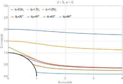
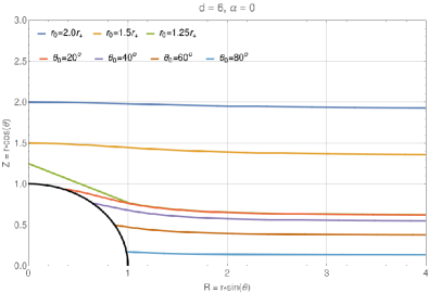
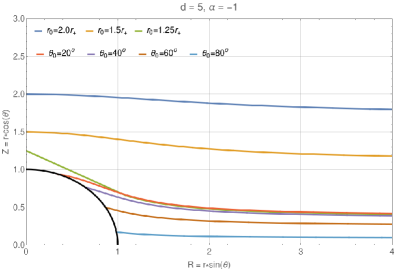
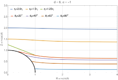
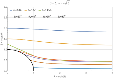
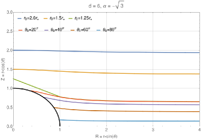
Figure 1: Static configurations of the BDBH system with a nonextremal black hole for $d$ equal to $5$ and $6$. The spacetime dimension and the value of the coupling constant $\alpha$ are presented above each diagram. The parameters $r_{0}$ and $\theta_{0}$ corresponding to the particular brane locations are listed on the plots.

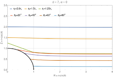
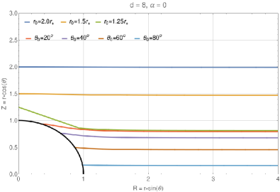
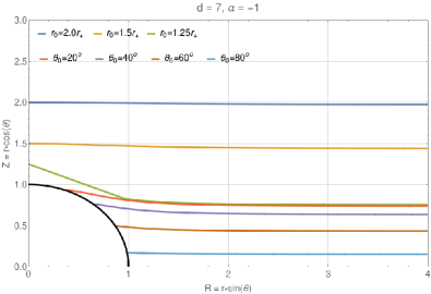
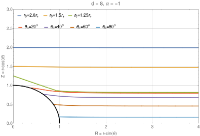
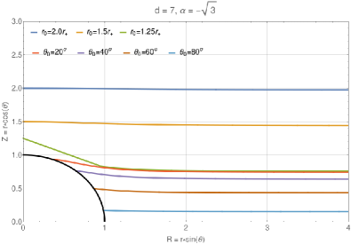
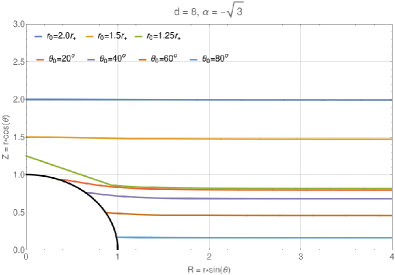
Figure 2: Static configurations of the BDBH system with a nonextremal black hole for $d$ equal to $7$ and $8$. The spacetime dimension and the value of the coupling constant $\alpha$ are presented above each diagram. The parameters $r_{0}$ and $\theta_{0}$ corresponding to the particular brane locations are listed on the plots.

The static configurations of an extremal brane-dilaton black hole system are depicted in figure 3. Disregarding the values of $d$ and $\alpha$, there exists only one brane location which penetrates the horizon and it corresponds to the brane situated on the equator plane of the black hole, with $\theta_{0}=\frac{\pi}{2}$ and hence $\theta=\frac{\pi}{2}$. The remaining arrangements represent branes which do not have any common points with the horizon. Each of these branes is described by a different value of $r_{0}$. Similarly to the nonextremal case, the bend of the brane disconnected with a black hole becomes smaller nearby its event horizon as the dimensionality of the considered spacetime $d$ increases. The above facts are in accord with the conclusions gained in four-dimensions, where the dilaton black hole - domain wall (brane) system was studied mod03 . Using the scalar field with various potentials, i.e., $\phi^{4}$ and sine-Gordon ones, the domain wall behavior in the spacetime of charged dilaton black hole was simulated numerically. The conclusion was that for the extremal charged dilaton black hole one always obtained the expulsion of the domain wall.

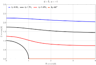
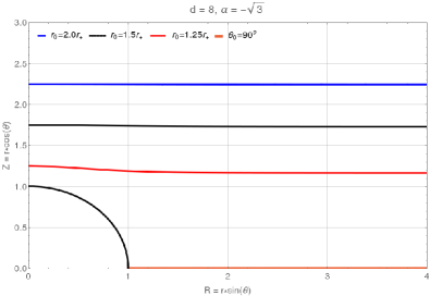
Figure 3: Static configurations of the BDBH system with an extremal black hole. The spacetime dimension $d$ and the value of the coupling constant $\alpha$ are presented above each diagram. The parameters $r_{0}$ and $\theta_{0}$ corresponding to the particular brane locations are listed on the plots.

4 Evolution of the brane-dilaton black hole system

Our further investigations concentrated on the dynamics of the BDBH system. The tension of the domain wall was assumed to be small which allowed us to ignore its self-gravitation effect.

4.1 Theoretical model

When describing the brane, we confined our attention to a scalar effective field theory with a quadratic potential of the scalar field $\Phi$ given by the relation

$$V\left(\Phi\right)=\frac{{\lambda}}{4}\Big{(}\Phi^{2}-\eta^{2}\Big{)}^{2},$$ (31)

where the parameters are related to the tension of a domain wall solution in a flat space $\sigma\approx\sqrt{\lambda}\eta^{3}$ and its thickness $l\approx(\sqrt{\lambda}\eta)^{-1}$. In contrast to the analysis of the static configurations of the examined system conducted in the preceding section, the effective field theory approach employed in investigations of the dynamical case allowed us to study not only an infinitely thin brane, but also branes of bigger thicknesses.

The equation of motion of the domain wall intersecting the dilaton black hole completely immersed in the higher-dimensional spacetime yields

$$\nabla_{\mu}\nabla^{\mu}\Phi-\frac{\partial V}{\partial\Phi}=0.$$ (32)

If one assumes an $O(d-2)$-rotational symmetry around the axis perpendicular to the equatorial plane of the considered black hole, then the following explicit form of the equation of motion arises:

$$\frac{-1}{f_{1}f_{2}^{\;1-\gamma(d-3)}}\;\partial_{t}^{2}\Phi+\frac{1}{r^{d-2}f_{2}^{\;\gamma}}\ \partial_{r}\Big{(}r^{d-2}f_{1}f_{2}\partial_{r}\Phi\Big{)}+\frac{1}{r^{2}\left(\sin\theta\right)^{d-3}}\;\partial_{\theta}\Big{[}\left(\sin\theta\right)^{d-3}\partial_{\theta}\Phi\Big{]}-\frac{\partial V}{\partial\Phi}=0.$$ (33)

Our main aim was to examine the potential recoil of the dilaton black hole from the brane during a dynamical process, at the beginning of which the brane intersecting the black hole acquires an initial velocity. Therefore, $\Phi$ and $\partial_{t}\Phi$ for $t=0$ are given by a static kink profile boosted in the direction of the symmetry axis fla06a . Namely, one has

$$\Phi_{v}=\eta\tanh\Bigg{(}\sqrt{\frac{{\lambda}}{2}}\eta\frac{r\cos\theta-vt}{\sqrt{1-v^{2}}}\Bigg{)},$$ (34)

where $v$ is constant.

At infinity, the field describing the brane reduces to the case of a flat spacetime form given by the relation (34), while the regularity conditions at the symmetry axis and on the black hole event horizon are

$$\frac{\partial\Phi}{\partial\theta} = 0\quad\textrm{at }\theta=0,\pi,$$ (35)

$$\frac{\partial\Phi}{\partial t} = 0\quad\textrm{at }r=r_{+}.$$

4.2 Numerical computations

The equation of motion of the scalar field representing the brane (33) was solved using the collocation spectral method Boyd in the spatial directions $r$ and $\theta$. The temporal evolution was conducted via a finite difference scheme based on three adjacent $t=const.$ hypersurfaces.

The applied pseudospectral method required writing the equation to be solved using a polynomial expansion of an unknown function at the so-called collocation points. The points were spread on a grid, which spanned from $-1$ to $1$ in the spectral directions, which in the considered case were $r$ and $\theta$.

The general form of $\Phi$ was chosen as an expansion in terms of the Chebyshev polynomials of the first kind

$$\Phi\big{(}t,y(r),x(\theta)\big{)} = \sum\limits_{m=0}^{M}\sum\limits_{n=0}^{N}\varphi_{mn}(t)\ T_{m}(y)\ T_{n}(x),$$ (36)

where $y=\frac{r-2r_{+}-1}{r+1}$ and $x=\cos\theta$ are the independent spatial variables rescaled to the range $[-1,1]$, which is necessary for applying the pseudospectral method. The time dependent expansion coefficients were denoted as $\varphi_{mn}$. The applied expansion involved $50$ Chebyshev polynomials in each of the two spatial directions. The collocation points were of the Gauss-Lobatto type, i.e, they were spread on the computational grid, in each of the spectral directions, according to a prescription

$$z_{k} = -\cos\frac{k\pi}{K},$$ (37)

where $k=0,\dots,K$, $z$ stands for either $y$ or $x$ and $K$ denotes $M$ or $N$, respectively.

The equation of motion of $\Phi$ (33) was reduced by applying the expansion (36) to the evolution equation of the expansion coefficients $\varphi_{mn}$ and obtained the form

$$\sum\limits_{m}\sum\limits_{n}\ddot{\varphi}_{mn}(t)\ T_{m}(y)\ T_{n}(x)-\frac{(1-y)^{d}f_{1}f_{2}^{\;1-\gamma(d-2)}}{2(r_{+}+1)(2r_{+}+1+y)^{d-2}}\sum\limits_{m}\sum\limits_{n}\varphi_{mn}(t)\ T_{n}(x)\ L_{m}(y)+$$

$$-\frac{(1-y)^{2}~{}f_{1}f_{2}^{1-\gamma(d-3)}}{(2r_{+}+1+y)^{2}}\sum\limits_{m}\sum\limits_{n}\varphi_{mn}(t)\ T_{m}(y)\ L_{n}(x)+f_{1}f_{2}^{1-\gamma(d-3)}~{}\frac{dV}{d\Phi}=0,\hskip 21.33955pt$$ (38)

where a dot is a derivative with respect to the $t$-coordinate and the auxiliary quantities are the following:

$$L_{m}(y) = \frac{(2r_{+}+1+y)^{d-3}\left[d-2-\frac{(d-4)(2r_{+}+1+y)}{1-y}\right]}{2(r_{+}+1)(1-y)^{d-4}}\ f_{1}f_{2}\ \partial_{y}T_{m}(y)+$$ (39)

$$+\frac{(2r_{+}+1+y)^{d-2}}{2(r_{+}+1)(1-y)^{d-4}}\Big{[}(\partial_{y}f_{1}f_{2}+f_{1}\partial_{y}f_{2})\ \partial_{y}T_{m}(y)+f_{1}f_{2}\ \partial^{2}_{y}T_{m}(y)\Big{]},$$

$$L_{n}(x) = \left(2-d\right)x\ \partial_{x}T_{n}(x)+\left(1-x^{2}\right)\partial_{x}^{2}T_{n}(x).$$ (40)

The equation (38) was written at each of the collocation points (37) separately. The resulting system of algebraic equations for the unknown $\varphi_{mn}$ was solved on each time step with the use of the LU decomposition method nrF .

The pseudospectral method provides an exact solution at the collocation points. Since the overall solution is approximated by a set of polynomials, bumps can appear in the regions between the points. They are an artifact of the numerical scheme. The density of the grid, i.e., the amount of collocation points used in our setup ($50$ in each spatial direction), ensured a very good accuracy of the obtained outcomes and facilitated their interpretation. It was also sufficient for modeling the step-type profile of the scalar field (34), which was necessary for reflecting the existence of the brane in the spacetime.

4.3 Dynamical behavior

The location of the brane in the spacetime was determined taking into account the values of the energy density of the scalar field $\Phi$

$$T_{0}^{\;0}=\frac{1}{f_{1}f_{2}^{\;1-\gamma(d-3)}}\big{(}\partial_{t}\Phi\big{)}^{2}+\frac{1}{4}f_{1}f_{2}^{\;1-\gamma}\big{(}\partial_{r}\Phi\big{)}^{2}+\frac{1}{r^{2}}\big{(}\partial_{\theta}\Phi\big{)}^{2}+\frac{1}{2}V(\Phi).$$ (41)

The results of the computations are presented through series of snapshots of the temporal evolution of the brane-black hole system. Each of the plots shows the energy density of the scalar field (41) within the black hole spacetime in cylindrical coordinates. The locations of the black hole horizons and the number of the evolution time step are shown on each diagram.

The investigated spacetime dimensions were $4$, $5$, $6$, $7$ and $8$. The brane thickness $l$ was set as $0.1$, $0.3$ and $0.4$, while its initial velocity $v$ was assumed to be equal to $0.1$, $0.3$ and $0.7$. Similarly to the case of static configurations of the BDBH system described in section 3, three values of the dilatonic constant $\alpha$ were considered, namely $-\sqrt{3}$, $-1$ and $0$. The constant $\eta$ was equal to $0.1$ in all simulations, which in addition to the value of $l$ determined the tension of the domain wall in each of the investigated cases.

Figures 4–7 present the dependence of the dynamical behavior of the brane-black hole system on $d$, $l$, $v$ and $\alpha$, respectively, in the case of a nonextremal black hole with $r_{-}=0.1$ and $r_{+}=0.5$. In all cases, the plane within which the brane was located initially divided the black hole into two hemispheres. Since the brane acquired a non-zero velocity at the beginning of the investigated process, with the passage of time it moved in a specific direction. Such a situation can also be interpreted as a black hole being expelled from the brane.

(a)

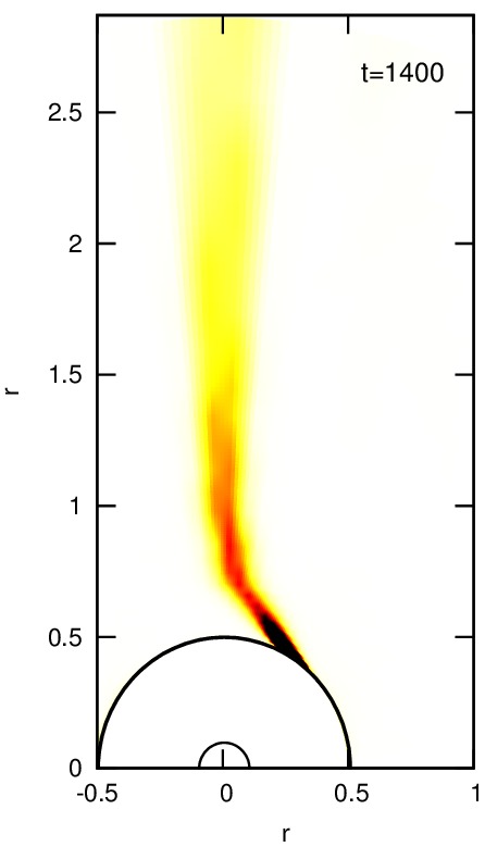
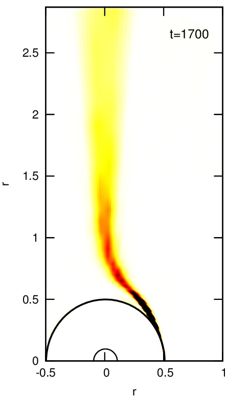
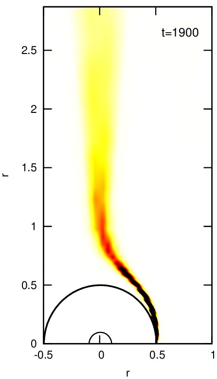
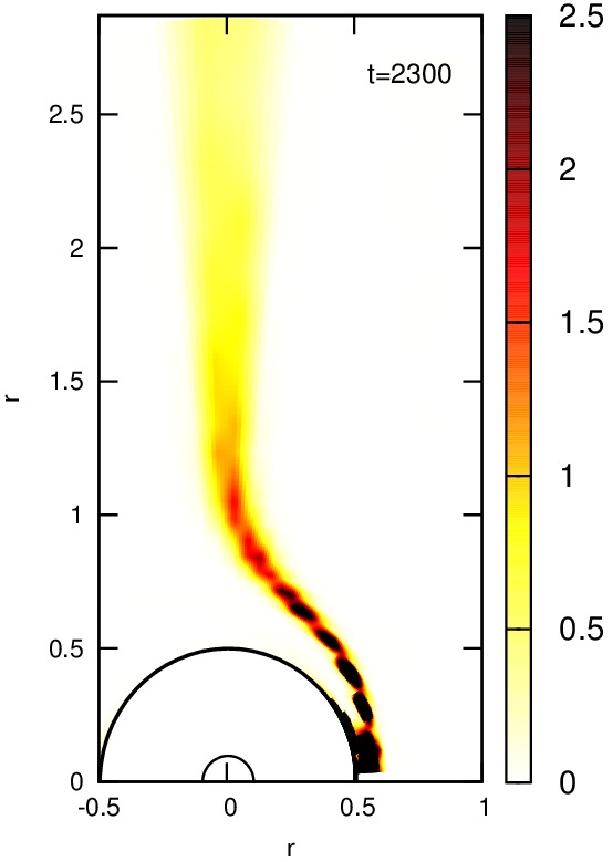
(b)

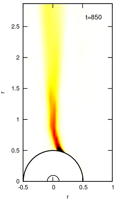
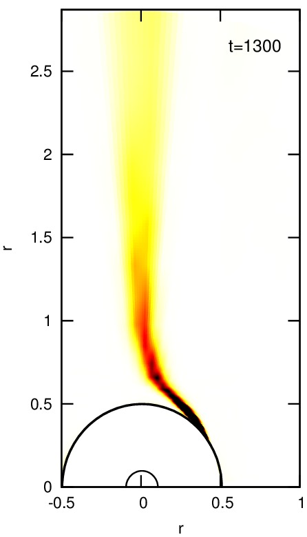
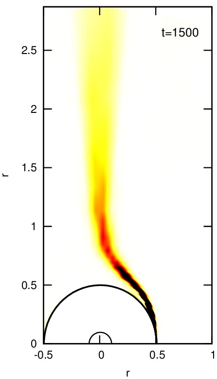
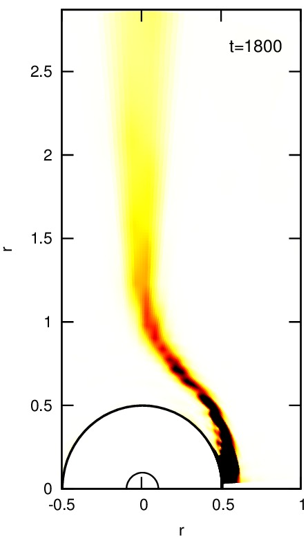
(c)

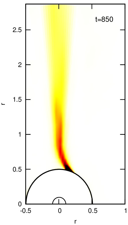
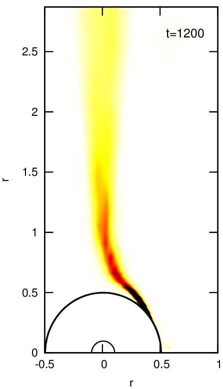
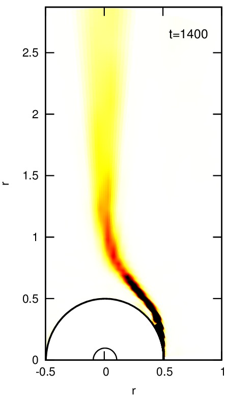
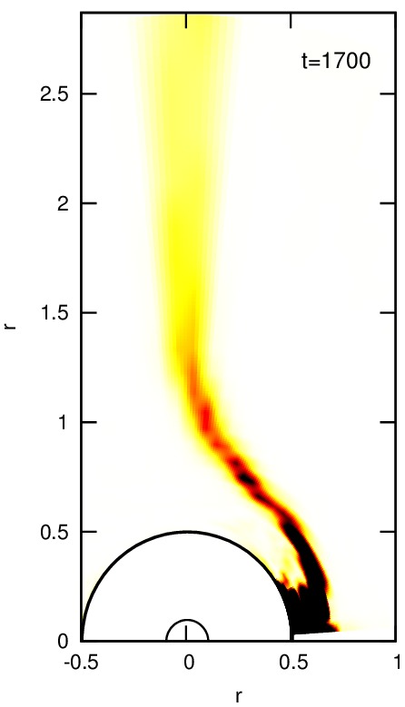
(d)

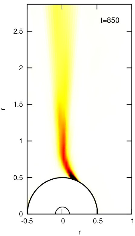
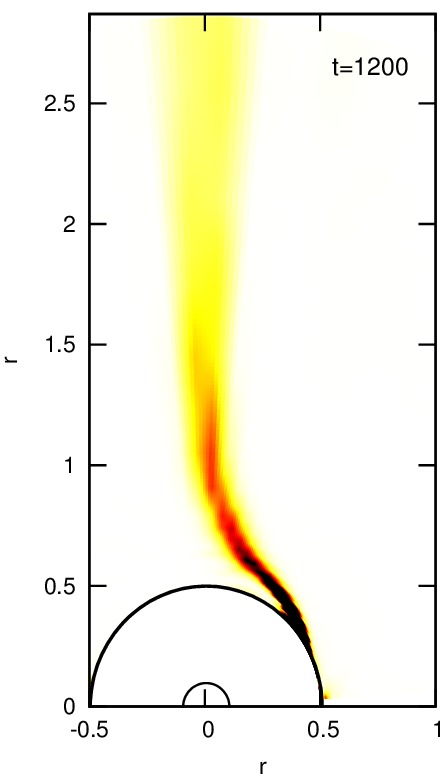
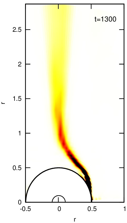
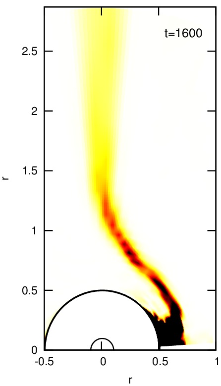
Figure 4: The evolution of the BDBH system with the nonextremal black hole for $d$ equal to (a) $4$, (b) $5$, (c) $6$ and (d) $7$. The remaining parameters were set as $l=0.1$, $v=0.1$ and $\alpha=-1$.

The research conducted for a BDBH system containing a nonextremal black hole revealed that the expulsion appears earlier for larger $d$ and the black hole is expelled earlier from a thicker brane (with bigger $l$). The radius of the area of the brane deformation is bigger for a thicker brane, it moves away from the initial position within a larger distance from the black hole. The energy density associated with a thick brane is smaller in comparison to a thin brane. Bigger initial velocity of the brane results in an earlier expulsion of the black hole and causes an increase of the radius of the area of the brane deformation nearby the black hole. The dynamics of the studied brane-black hole system does not depend on the value of $\alpha$.

(a)

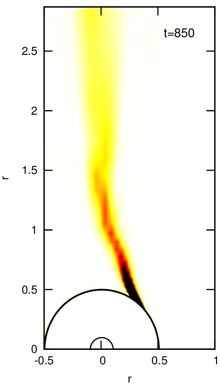
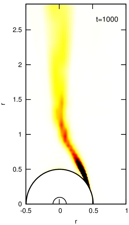
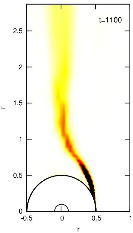
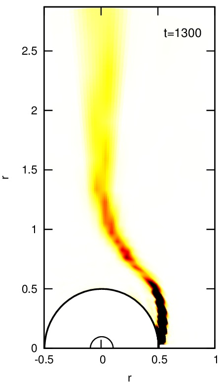
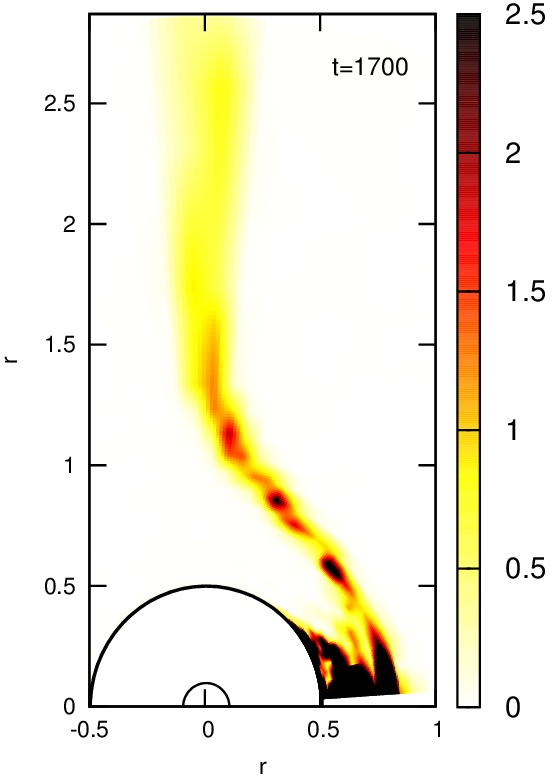
(b)

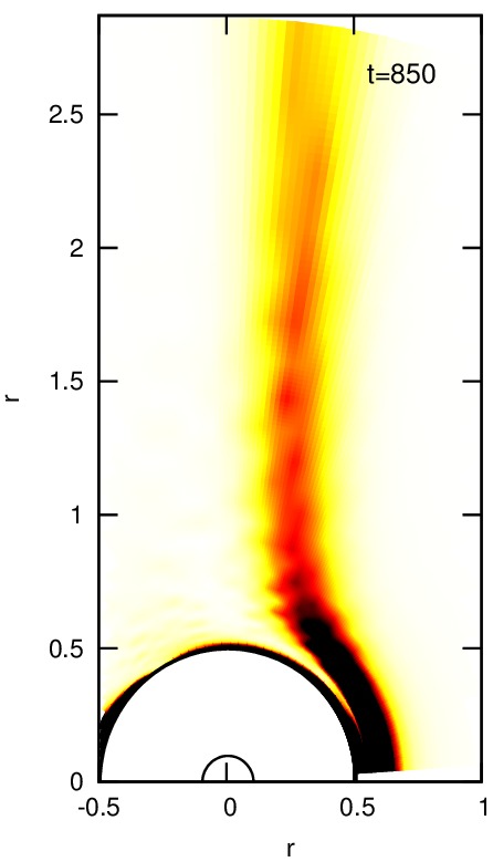
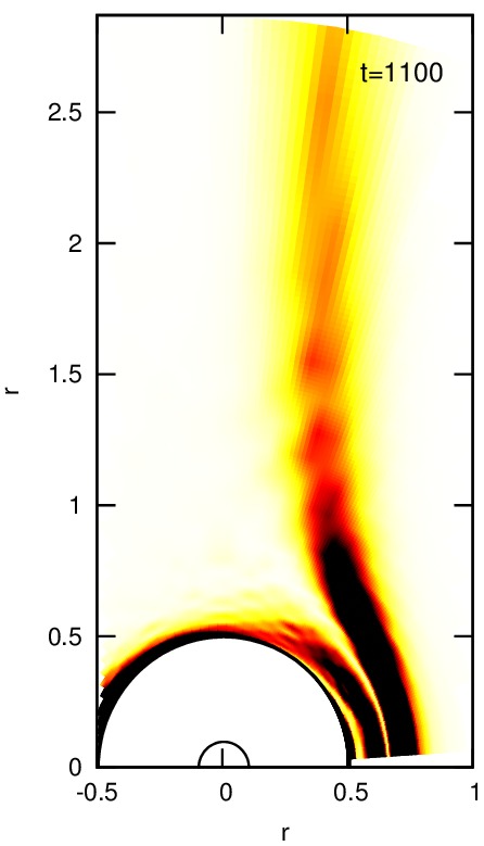
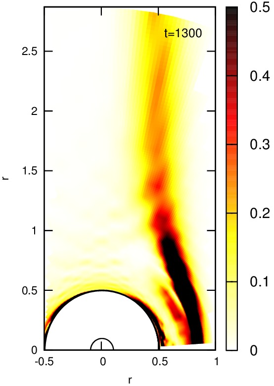
(c)

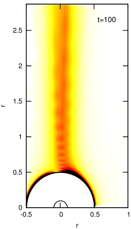
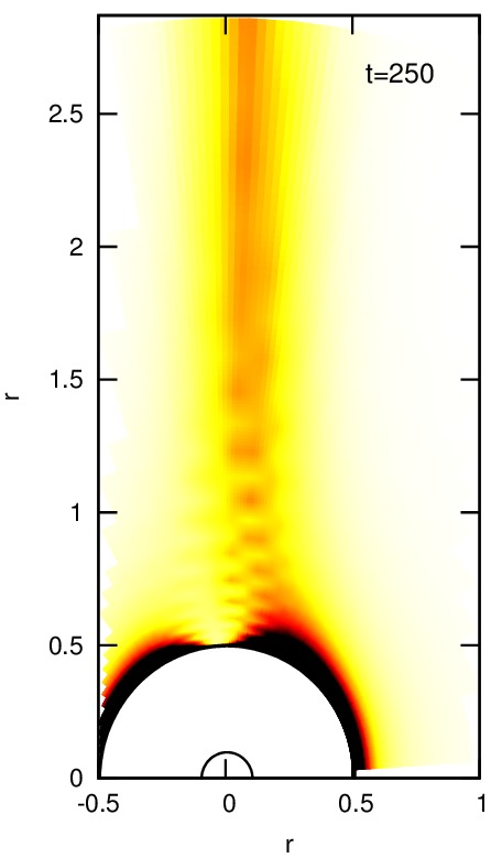
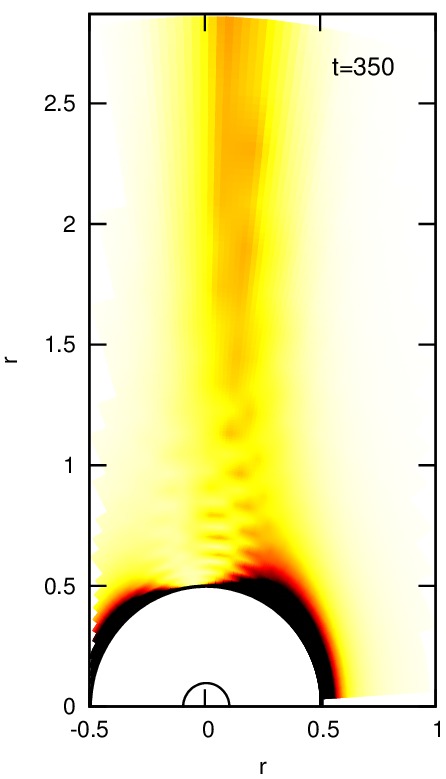
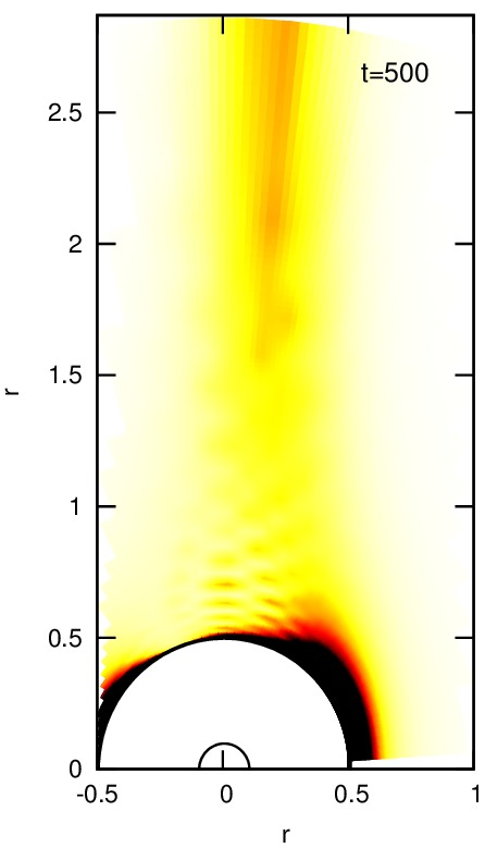
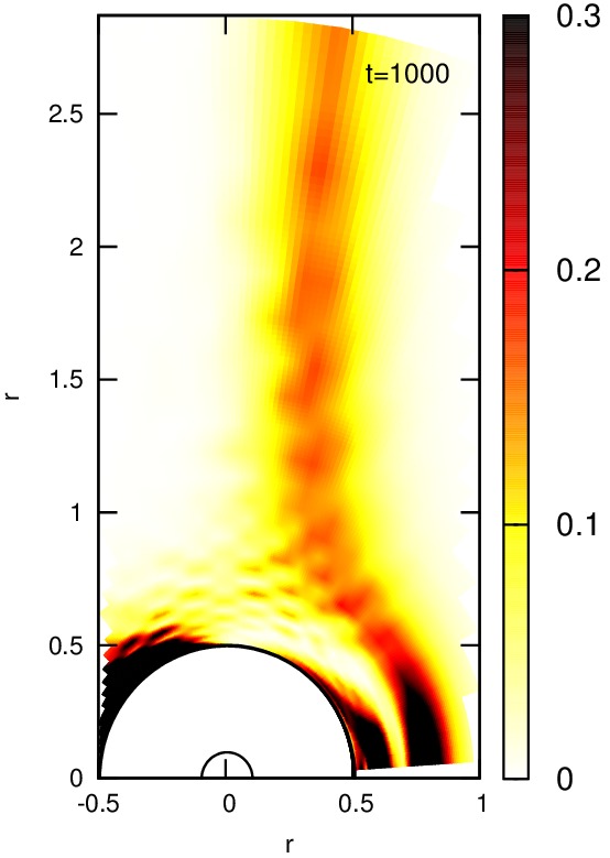
Figure 5: The evolution of the BDBH system with the nonextremal black hole for $l$ equal to (a) $0.1$, (b) $0.3$ and (c) $0.4$. The remaining parameters were set as $d=5$, $v=0.3$ and $\alpha=0$.

(a)

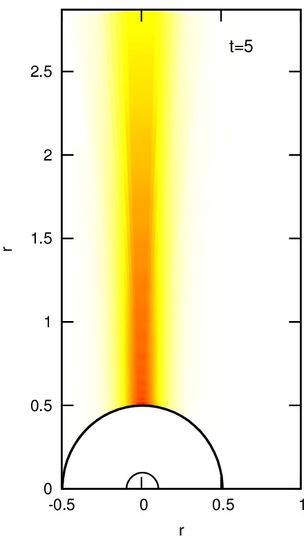
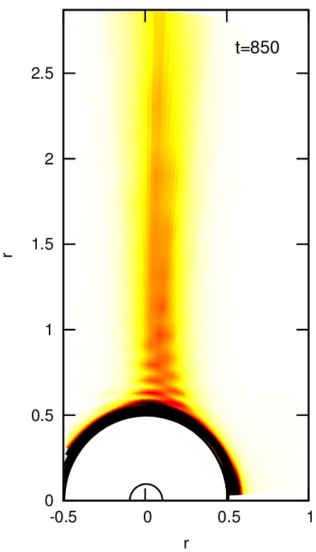
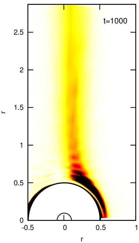
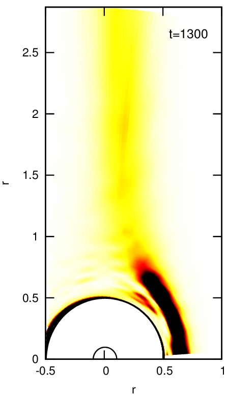
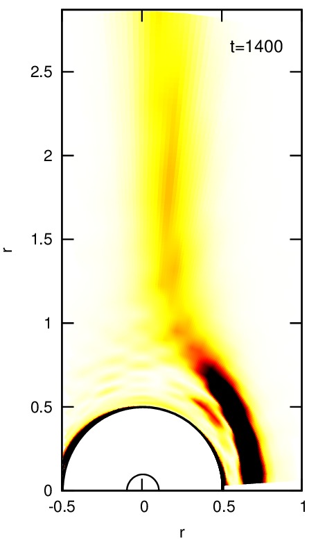
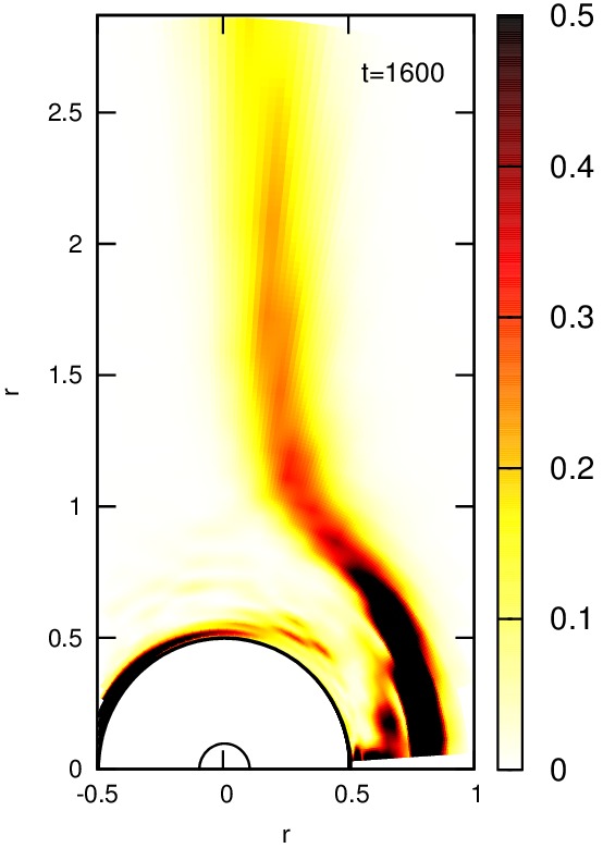
(b)

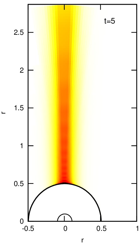
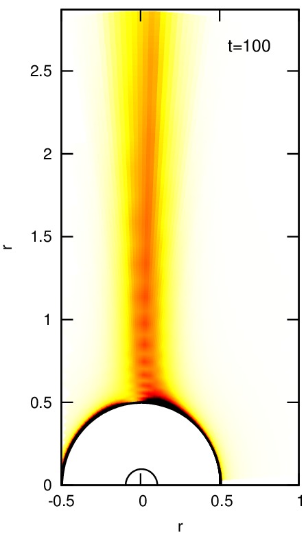
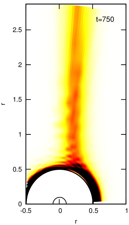
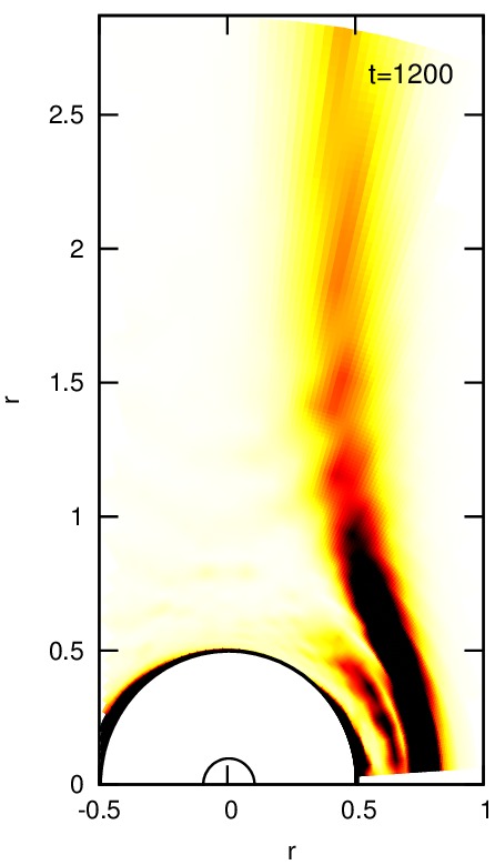
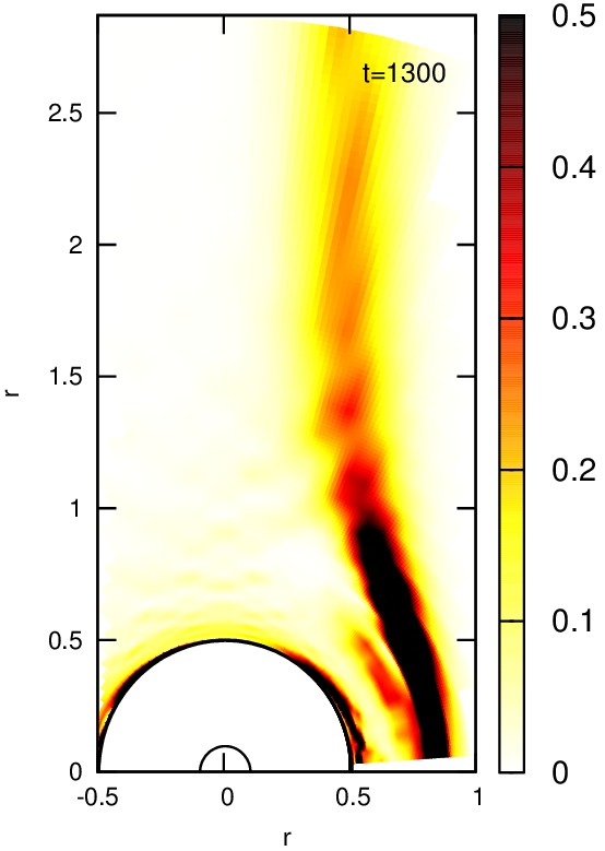
(c)

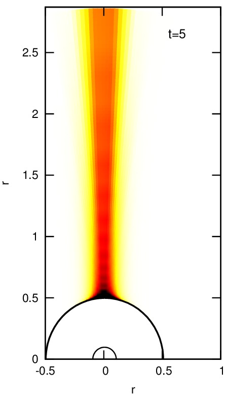
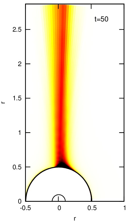
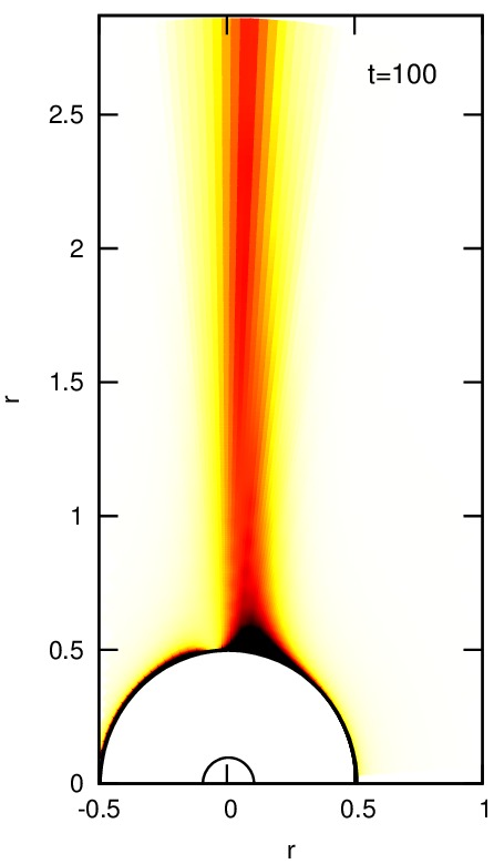
Figure 6: The evolution od the BDBH system with the nonextremal black hole for $v$ equal to (a) $0.1$, (b) $0.3$ and (c) $0.7$. The remaining parameters were set as $d=5$, $l=0.3$ and $\alpha=-1$.

(a)

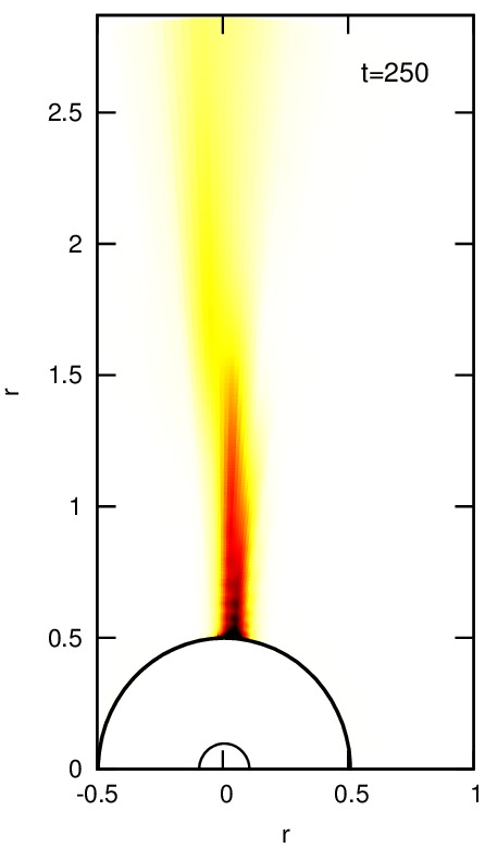
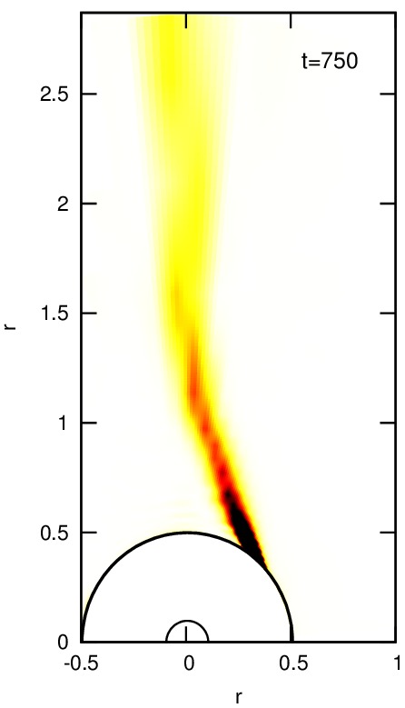
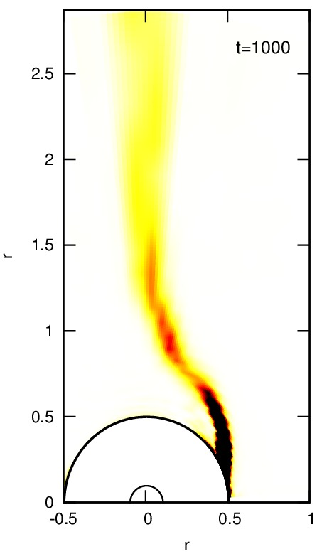
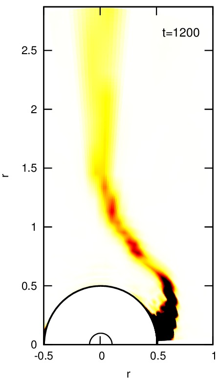
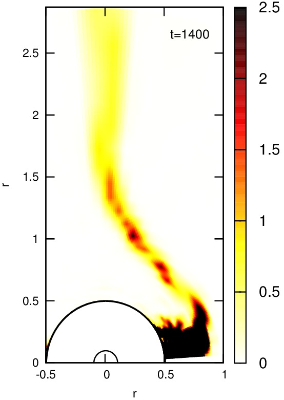
(b)

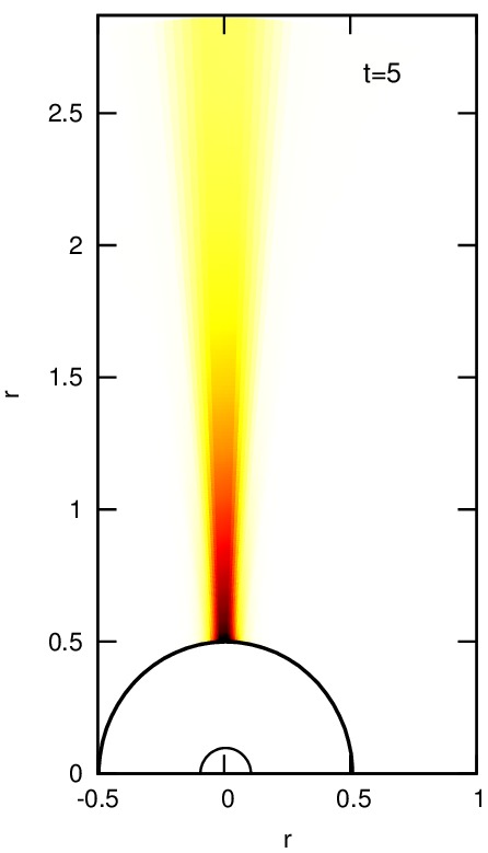
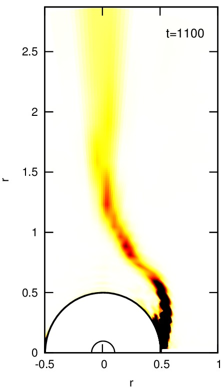
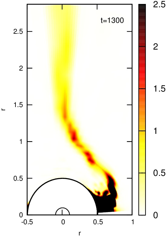
Figure 7: The evolution of the BDBH system with the nonextremal black hole for $\alpha$ equal to (a) $-1$ and (b) $0$. The remaining parameters were set as $d=7$, $l=0.1$ and $v=0.3$.

The evolution of the examined system was also followed for an extremal black hole with $r_{-}=r_{+}=0.5$. The outcomes were qualitatively the same as in the nonextremal case, the only difference was that the expulsion appeared a bit earlier in the extremal case.

5 Conclusions

In our paper we pay attention to static configurations and a dynamical evolution of the system consisting of a higher-dimensional spherically symmetric dilaton black hole and a Dirac-Goto-Nambu type brane. Due to the employed theoretical descriptions of the brane in the static and dynamical cases, the former analysis corresponds to an infinitely thin brane, while the latter covers also branes of non-negligible thicknesses.

It has been established gar91 ; cam90 ; sha91 ; hol92 that the classical black hole solutions of Einstein-Maxwell gravity have quite new features when the theory is modified by the introduction of the low-energy string corrections to the underlying action. The key property of the aforementioned actions is bounded with the nontrivial coupling of the dilaton field with gravity and the field strength of Maxwell or Yang-Mills gauge fields. The charged black hole or black brane solutions in the low-energy string theory differ to the great extent in comparison to those solutions received in ordinary Einstein-Maxwell or Einstein-Yang-Mills theories. For instance, their thermodynamical properties are quite unconventional, i.e., extremal dilaton black holes have zero entropy but its temperature is non-zero pre91 . Moreover, their properties connected with late-time behavior of scalar fields in their backgrounds mod01a ; mod01b , decay of hair on them rog07 ; rog08 , thermodynamical properties and inequalities among mass, charge and angular momentum rog94 ; rog95 ; rog00 ; rog02 ; rog02b ; rog97 ; rog98 ; rog14 , uniqueness theorems rog99 ; rog ; rog10 and dynamical collapse process and formation of singularities bor11 ; nak12prd ; nak12cqg ; nak15 , are quite not trivial.

In order to have the full insight in the properties of the aforementioned black object it is interesting to elaborate the problem of a static and dynamical behavior of the simple brane in the spacetime of higher dimensional dilaton black hole. The first studies of such a problem were presented in mod03 , where the existence of a brane (domain wall) was mimicked by the real scalar field with the $\phi^{4}$ and sine-Gordon potentials. The previous investigations were restricted to the four-dimensional case and thick branes. It was revealed that in the case of the extremal dilaton black hole one always obtained an expulsion of the domain wall from the black hole in question.

Our studies were conducted for three values of the coupling constant $\alpha$, which referred to the uncoupled dilaton field, the low-energy limit of the string theory and dimensionally reduced Klein-Kaluza theory. It turns out that the value of the dilaton coupling does not influence the static configurations. However, the brane location in the black object spacetime is connected with the dimensionality of the spacetime in question. The brane bend in the nearby of the black object event horizon disappears closer to it as the dimensionality of the bulk increases. The possible explanation of this fact is connected with the gravity feature which can penetrate the additional dimensions. The same force (bounded with the black hole mass) ought to act in the additional dimensions and therefore is weaker in comparison to the four-dimensional case. Thus, one can draw a conclusion that, the larger dimensionality of the spacetime manifold one considers, the weaker force is exerted on the brane in question. It seems to be the common feature of the higher-dimensional systems. The very similar behavior was noticed in studies of the absorption cross section, for massive Dirac field in higher dimensional black hole spacetime. Namely, $|A|^{2}$ for the bulk massive Dirac fermions in the spacetime of $(n+4)$-dimensional Schwarzschild black hole decreases with the increase of the dimensionality of the spacetime rog09 . For the lower energy spectrum we have the same conclusion concerning the higher dimensional black hole luminosity.

In the case of the extremal dilaton black hole-brane configurations, one always gets expulsion of the brane from the black objects, disregarding dimension of the spacetime and the coupling constant of the theory under consideration. This fact confirms the previous results obtained for the four-dimensional dilaton black hole-brane system mod03 . In four dimensions the same effect was also revealed for the Abelian Higgs cosmic strings and extremal dilaton black holes mod98 ; mod99 .

The dynamical evolution of the considered system was elaborated as the series of snapshots of the temporal evolution of the brane-black hole, for nonextremal and extremal black objects. The energy density of the scalar field was examined in the black hole spacetime in cylindrical coordinates. We have considered various spacetime dimensions, i.e., 4, 5, 6, 7 and 8, as well as, the changes of the brane thickness. In the nonextremal case, it turned out that the black hole is expelled earlier from the brane in the bulk of a larger dimension and when the brane is thicker. Namely, the radius of the area of the brane deformation has a bigger value for a thicker brane. It moves from the initial position to a larger distance outside the black hole in question. As far as the energy is concerned, the energy density of the thick brane is smaller than for a thin one. Moreover, it happens that the bigger initial velocity we examine, the earlier expulsion of the black hole we observe. The large value of velocity causes the increase of the area of the brane deformation in the vicinity of the black object. Similarly to the static configurations, the dilatonic coupling value does not influence the process in question.

On the other hand, for the extremal dilaton black hole all the aforementioned conclusions are also valid. The only difference is that the expulsion takes place a little bit earlier than in the nonextremal case.

The current studies could be broadened in several directions, the examples of which are the following. One of them is disregarding the restriction of the codimension-one brane and investigating other values of the bulk spacetime and the brane relative dimensionalities. An assumption of spherical symmetry could be also weakened so that static and stationary axisymmetric spacetimes could be considered.

- (1)
- (2)
- (3) N. Arkani-Hamed, S. Dimopoulos and G. R. Dvali, The hierarchy problem and new dimensions at a millimeter, Phys. Lett. B 429 (1998) 263.
- (4) N. Arkani-Hamed, S. Dimopoulos and G. R. Dvali, Phenomenology, astrophysics, and cosmology of theories with submillimeter dimensions and TeV scale quantum gravity, Phys. Rev. D 59 (1999) 086004.
- (5) L. Randall and R. Sundrum, Large Mass Hierarchy from a Small Extra Dimension, Phys. Rev. Lett. 83 (1999) 3370.
- (6) L. Randall and R. Sundrum, An Alternative to Compactification, Phys. Rev. Lett. 83 (1999) 4690.
- (7) N. Tanahashi and T. Tanaka, Black Holes in Braneworlds Models, Prog. Theor. Phys. Suppl. 189 (2011) 227.
- (8) V. P. Frolov, Merger transitions in brane-black hole systems: Criticality, scaling, and self-similarity, Phys. Rev. D 74 (2006) 044006.
- (9) B. Kol, Topology change in general relativity, and the black-hole black-string transition, JHEP 10 (2005) 049.
- (10) B. Kol, The phase transition between caged black holes and black strings, Phys. Reports 422 (2006) 119.
- (11) D. Mateos, R. C. Myers and R. M. Thomson, Holographic Phase Transitions with Fundamental Matter, Phys. Rev. Lett. 97 (2006) 091601.
- (12) D. Mateos, R. C. Myers and R. M. Thomson, Thermodynamics of the brane, JHEP 05 (2007) 067.
- (13) V. G. Czinner, Axisymmetric Dirac-Nambu-Goto branes on Myers-Perry black hole backgrounds, Phys. Rev. D 88 (2013) 124029.
- (14) S. Dimopoulos and G. L. Landsberg, Black holes at the LHC, Phys. Rev. Lett. 87 (2001) 161602.
- (15) S. B. Giddings and S. Thomas, High energy colliders as black hole factories: The end of short distance physics, Phys. Rev. D 65 (2002) 056010.
- (16) A. Vilenkin and E. P. Shellard, Cosmic strings and other topological defects, (Cambridge University Press 1994).
- (17) S. Higaki, A. Ishibashi, and D. Ida, Instability of a membrane intersecting a black hole, Phys. Rev. D 63 (2000) 025002.
- (18) Y. Morisawa, R. Yamazaki, D. Ida, A. Ishibashi, and K. Nakao, Thick domain walls intersecting a black hole, Phys. Rev. D 62 (2000) 084022.
- (19) Y. Morisawa, R. Yamazaki, D. Ida, A. Ishibashi, and K. Nakao, Thick domain walls around a black hole, Phys. Rev. D 67 (2003) 025017.
- (20) M. Rogatko, Dilaton black holes on thick branes, Phys. Rev. D 64 (2001) 064014.
- (21) R. Moderski and M. Rogatko, Thick domain walls and charged dilaton black holes, Phys. Rev. D 67 (2003) 024006.
- (22) R. Moderski and M. Rogatko, Reissner-Nordström black holes and thick domain walls, Phys. Rev. D 69 (2004) 084018.
- (23) R. Moderski and M. Rogatko, Thick domain walls in AdS black hole spacetimes, Phys. Rev. D 74 (2006) 044002.
- (24) M. Rogatko, Cosmological black holes on branes, Phys. Rev. D 69 (2004) 044022.
- (25) A. Flachi and T. Tanaka, Escape of black holes from the brane, Phys. Rev. Lett. 95 (2005) 161302.
- (26) A. Flachi, O. Pujolas, M. Sasaki and T. Tanaka, Black holes escaping from domain walls, Phys. Rev. D 73 (2006) 125017.
- (27) A. Flachi, O. Pujolas, M. Sasaki and T. Tanaka, Critical escape velocity of black holes from branes, Phys. Rev. D 74 (2006) 045013.
- (28) A. Flachi and T. Tanaka, Branes and black holes collision, Phys. Rev. D 76 (2007) 025007.
- (29) A. Chamblin and D. M. Eardley, Puncture of gravitating domain walls, Phys. Lett. B 475 (2000) 46.
- (30) D. Stojkovic, K. Freese and G. D. Starkman, Holes in the walls: Primordial black holes as a solution to the cosmological domain wall problem, Phys. Rev. D 72 (2005) 045012.
- (31) V. G. Czinner and A. Flachi, Curvature corrections and topology change transition in brane-black hole systems: A perturbative approach, Phys. Rev. D 80 (2009) 104017.
- (32) V. G. Czinner, Thick-brane solutions and topology change transition on black hole backgrounds, Phys. Rev. D 82 (2010) 024035.
- (33) V. G. Czinner, A topologically flat thick 2-brane on higher-dimensional black hole backgrounds, Phys. Rev. D 83 (2011) 064026.
- (34) V. Balek and B. Novotny, Evolution of a black hole inhabited brane close to reconnection, Phys. Rev. D 83 (2011) 024013.
- (35) D. V. Gal’tsov, E. Yu. Melkumova and P. Spirin, Perforation of a domain wall by a point mass, Phys. Rev. D 89 (2014) 085017.
- (36) D. V. Gal’tsov, E. Yu. Melkumova and P. Spirin, Energy-momentum balance in a particle domain wall perforating collision, Phys. Rev. D 90 (2014) 125024.
- (37) G. W. Gibbons, K.-i. Maeda, Black holes and membranes in higher-dimensional theories with dilaton fields, Nucl. Phys. B 298 (1988) 741.
- (38) P. A. M. Dirac, An Extensible Model of the Electron, Proc. R. Soc. London, Ser. A 268 (1962) 57.
- (39) J. Nambu, Copenhagen Summer Symposium (1970), unpublished.
- (40) T.Goto, Merger Transitions in Brane-Black Hole Systems: Criticality, Scaling, and Self-Similarity, Prog. Theor. Phys. 46 (1971) 1560.
- (41) G. W. Gibbons, M. Rogatko, and A. Szypłowska, Decay of massive Dirac hair on a brane-world black hole, Phys. Rev. D 77 (2008) 064024.
- (42) M. Rogatko, and A. Szypłowska, Massive fermion emission from higher dimensional black holes, Phys. Rev. D 79 (2009) 104005.
- (43) G. W. Gibbons and M. Rogatko, Decay of Dirac hair around a dilaton black hole, Phys. Rev. D 77 (2008) 044034.
- (44) J. P. Boyd, Chebyshev and Fourier spectral methods, Dover Publications 2000, NY, USA.
- (45) W. H. Press, S. A. Teukolsky, W. T. Vetterling, B. P. Flannery, Numerical Recipes in Fortran 77, Cambridge University Press 1997, USA.
- (46) D.Garfinkle, G.T.Horowitz, and A.Strominger, Charged black holes in string theory, Phys. Rev. D 43 (1991) 3140.
- (47) B.A.Cambell, M.J.Duncan, N.Kaloper, and K.A.Olive, Axion hair for Kerr black holes, Phys. Lett. B 251 (1990) 34.
- (48) A.Shapere, S.Trivedi, and F.Wilczek, Dual dilation dyons, Mod. Phys. Lett. A 6, (1991) 2677.
- (49) C.F.E.Holzhey and F.Wilczek, Black holes as elementary particles, Nucl. Phys. B 380 (1992) 447.
- (50) J.Preskill, P.Schwarz, A.Shapere, S.Trivedi, and F.Wilczek, Limitations on the statistical description of black holes, Mod. Phys. Lett. A 6, (1991) 2353.
- (51) R.Moderski and M.Rogatko, Late-time evolution of a charged massless scalar field in the spacetime of a dilaton black hole, Phys. Rev. D 63 (2001) 084014.
- (52) R.Moderski and M.Rogatko, Late-time evolution of a self-interacting scalar field in the spacetime of a dilaton black hole, Phys. Rev. D 64 (2001) 044024.
- (53) M.Rogatko, Decay of massive scalar hair in the background of a dilaton gravity black hole, Phys. Rev. D 75 (2007) 104006.
- (54) G.W.Gibbons and M.Rogatko, Decay of Dirac hair around a dilaton black hole, Phys. Rev. D 77 (2008) 044034.
- (55) M.Rogatko, Stationary axisymmetric axion-dilaton black holes mass formulae, Class. Quant. Grav. 11 (1994) 689.
- (56) M.Rogatko, The Bogomolnyi-type bound in axion - dilaton gravity, Class. Quant. Grav. 12 (1995) 3115.
- (57) M.Rogatko, Positivity of the Bondi energy in Einstein-Maxwell axion-dilaton gravity, Class. Quant. Grav. 17 (2000) 4577.
- (58) M.Rogatko, Positivity of energy in Einstein-Maxwell axion-dilaton gravity, Class. Quant. Grav. 19 (2002) 5063.
- (59) M.Rogatko, Physical process version of the first law of thermodynamics for black holes in Einstein-Maxwell axion-dilaton gravity, Class. Quant. Grav. 19 (2002) 3821.
- (60) M.Rogatko, The staticity problem for non-rotating black holes in Einstein-Maxwell axion-dilaton gravity, Class. Quant. Grav. 14 (1997) 2425.
- (61) M.Rogatko, Extrema of mass, first law of black hole mechanics, and a staticity theorem in Einstein-Maxwell-axion-dilaton gravity, Phys. Rev. D 58 (1998) 044011.
- (62) M.Rogatko, Mass, angular momentum, and charge inequalities for black holes in Einstein-Maxwell-axion-dilaton gravity, Phys. Rev. D 89 (2014) 044020.
- (63) M. Rogatko, Uniqueness theorem for static dilaton black holes, Phys. Rev. D 59 (1999) 104010.
- (64) M. Rogatko, Uniqueness theorem for static dilaton black holes, Class. Quant. Grav. 19 (2002) 875.
- (65) M. Rogatko, Uniqueness theorem for stationary axisymmetric black holes in Einstein-Maxwell-axion-dilaton gravity, Phys. Rev. D 82 (2010) 044017.
- (66) A. Borkowska, M. Rogatko, and R. Moderski, Collapse of charged scalar field in dilaton gravity, Phys. Rev. D 83 (2011) 084007.
- (67) A. Nakonieczna, M.Rogatko, and R. Moderski, Dynamical collapse of charged scalar field in phantom gravity, Phys. Rev. D 86 (2012) 044043.
- (68) A. Nakonieczna and M. Rogatko, Dilatons and the dynamical collapse of charged scalar field, Gen. Rel. Grav. 44 (2012) 3175.
- (69) A. Nakonieczna, M. Rogatko, and Ł. Nakonieczny, Dark sector impact on gravitational collapse of an electrically charged scalar field, JHEP 11 (012) 2015.
- (70) M. Rogatko and A. Szypłowska, Massive fermion emission from higher dimensional black holes, Phys. Rev. D 79 (2009) 104005.
- (71) R. Moderski and M. Rogatko, Abelian Higgs hair for electrically charged dilaton black holes, Phys. Rev. D 58 (1998) 124016.
- (72) R. Moderski and M. Rogatko, The question of Abelian Higgs hair expulsion from extremal dilaton black holes, Phys. Rev. D 60 (1999) 104040.