Submitted to IEEE Transactions on Signal Processing
Efficient L1-Norm Principal-Component Analysis via Bit Flipping

Abstract

It was shown recently that the $K$ L1-norm principal components (L1-PCs) of a real-valued data matrix $\mathbf{X}\in\mathbb{R}^{D\times N}$ ($N$ data samples of $D$ dimensions) can be exactly calculated with cost $\mathcal{O}(2^{NK})$ or, when advantageous, $\mathcal{O}(N^{dK-K+1})$ where $d=\mathrm{rank}(\mathbf{X})$, $K<d$ [1, 2]. In applications where $\mathbf{X}$ is large (e.g., “big” data of large $N$ and/or “heavy” data of large $d$), these costs are prohibitive. In this work, we present a novel suboptimal algorithm for the calculation of the $K<d$ L1-PCs of $\mathbf{X}$ of cost $\mathcal{O}(ND\mathrm{min}\{N,D\}+N^{2}(K^{4}+dK^{2})+dNK^{3})$, which is comparable to that of standard (L2-norm) PC analysis. Our theoretical and experimental studies show that the proposed algorithm calculates the exact optimal L1-PCs with high frequency and achieves higher value in the L1-PC optimization metric than any known alternative algorithm of comparable computational cost. The superiority of the calculated L1-PCs over standard L2-PCs (singular vectors) in characterizing potentially faulty data/measurements is demonstrated with experiments on data dimensionality reduction and disease diagnosis from genomic data.

Index Terms — Dimensionality reduction, data analytics, eigen-decomposition, L1 norm, L2 norm, machine learning, outlier resistance, principal component analysis, subspace signal processing.

I Introduction

Principal-Component Analysis (PCA) [4] has been a “mainstay” of signal processing, machine learning, pattern recognition, and classification [5, 6, 7] for more than a century. Numerous important applications of PCA can be found in the fields of wireless communications, computer networks, computer vision, image processing, bio-informatics/genomics, and neuroscience, to name a few. Broadly speaking, PCA seeks to calculate orthogonal directions that define a subspace wherein data presence is maximized. Traditionally, PCA quantifies data presence by the Frobenius (L2) norm of the projected data onto the subspace, or, equivalently, the Euclidean distance of the original data from their subspace representations (L2-norm of residual error). Herein, we will be referring to standard PCA as L2-PCA. Key strengths of L2-PCA are (i) its low-complexity implementation (quadratic in the number of data points) by means of singular-value decomposition (SVD) of the data matrix and (ii) the reliable approximation that it offers to the nominal principal data subspace, when calculated over sufficiently many clean/nominal or benign-noise corrupted data points.

In the advent of the big-data era, datasets often include grossly corrupted, highly deviating, irregular data points (outliers), due to a variety of causes such as transient sensor malfunctions, errors in data transmission/transcription, errors in training data labeling, and bursty-noise data corruption, to name a few [8, 9]. Regretfully, standard L2-PCA is well-known to be fragile in the presence of such faulty data, even when they appear in a vanishingly small fraction of the training set [10]. The reason is that the L2-norm objective of standard PCA (minimization of error variance or maximization of squared projection magnitude) gives squared importance on the magnitude of every datum, thus overemphasizing peripheral data points.

To remedy the impact of outliers, researchers from the fields of data analysis and signal processing have long focused on calculating subspaces of minimum absolute error deviations, instead of minimum error variances. Important early theoretical studies date back to the 1940s [11, 12, 13, 14]. In the past decade, there have been several L1-norm-based principal component calculators under the general label “L1-PCA” [15, 16, 17, 18, 23, 24, 25, 21, 19, 20, 26, 29, 27, 28, 22, 30, 31, 32, 33, 37, 36, 34, 35, 3]. In these works, researchers seek either to (i) minimize the aggregate absolute data representation error or (ii) maximize the aggregate absolute magnitude of the projected data points. For approach (i), it has been shown that the error surface is non-smooth and the problem non-convex, resisting attempts to reach an exact solution even with exponential computational cost [38]. Therefore, only suboptimal algorithms exist in the literature [15, 16, 17, 18]. For approach (ii), a problem known as maximum-projection L1-PCA, the works in [1, 2] proved that maximum-projection L1-PCA is not NP-hard for fixed data dimension $D$ and offered the first two optimal algorithms in the literature for exact calculation. Specifically, for a data record of size $N$, $\mathbf{X}\in\mathbb{R}^{D\times N}$, the first optimal algorithm solves L1-PCA exactly with complexity $\mathcal{O}(2^{NK})$; the second optimal algorithm solves L1-PCA exactly with complexity $\mathcal{O}(N^{\mathrm{rank}(\mathbf{X})K-K+1})$ where $K<\mathrm{rank}(\mathbf{X})$ is the desired number of L1-PCs. Before the results of [1, 2], several low-complexity suboptimal algorithms for L1-PCA existed in the literature [19, 20, 21, 22]. However, in lack of the optimal solution, no absolute performance evaluation of those algorithms with respect to the L1-PCA metric could be conducted until [1, 2] made the optimal value available. Today, optimal-solution-informed experimental studies indicate that the existing low-cost approximate algorithms for L1-PCA yield non-negligible performance degradation, in particular when more than one principal component is calculated.

In this present work, we introduce L1-BF, a bit-flipping based algorithm for the calculation of the $K$ L1-PCs of any rank-$d$ data matrix $\mathbf{X}\in\mathbb{R}^{D\times N}$ with complexity $\mathcal{O}(ND\mathrm{min}\{N,D\}+N^{2}(K^{4}+dK^{2})+NdK^{3})$. The proposed algorithm is accompanied by: (i) Formal proof of convergence and theoretical analysis of converging points; (ii) detailed asymptotic complexity derivation; (iii) theoretically proven performance guarantees; (iv) L1-PCA performance comparisons with state-of-the-art counterparts of comparable computational cost [19, 20, 21, 22]; and (v) outlier-resistance experiments on dimensionality reduction, foreground motion detection in surveillance videos, and disease diagnosis from genomic data. Our studies show that L1-BF outperforms all suboptimal counterparts of comparable cost with respect to the L1-PCA metric and retains high outlier-resistance similar to that of optimal L1-PCA. Thus, the proposed algorithm may bridge the gap between computationally efficient and outlier-resistant principal component analysis.

The rest of the paper is organized as follows. Section II presents the problem statement and reviews briefly pertinent technical background. Section III is devoted to the development and analysis of the proposed algorithm. Extensive experimental studies are presented in Section IV. A few concluding remarks are drawn in Section V.

II Problem Statement and Background

Given a data matrix ${\mathbf{X}}=[\mathbf{x}_{1},\mathbf{x}_{2},\ldots,\mathbf{x}_{N}]\in\mathbb{R}^{D\times N}$ of rank $d\leq\min\{D,N\}$, we are interested in calculating a low-rank data subspace of dimensionality $K<d$ in the form of an orthonormal basis $\mathbf{Q}_{L1}\in\mathbb{R}^{D\times K}$ that solves

$${\mathbf{Q}_{L1}=\underset{\begin{smallmatrix}\mathbf{Q}=[\mathbf{q}_{1},\ldots,\mathbf{q}_{K}]\in\mathbb{R}^{D\times K}\\ \mathbf{Q}^{\top}\mathbf{Q}=\mathbf{I}_{K}\end{smallmatrix}}{\mathrm{argmax}}\leavevmode\nobreak\ \sum_{k=1}^{K}\left\|\mathbf{X}^{\top}\mathbf{q}_{k}\right\|_{1}.}$$ (1)

In (1), $\left\|\cdot\right\|_{1}$ denotes the element-wise L1-norm of the vector/matrix argument that returns the sum of the absolute values of the individual entries. [1, 2] and [22] presented different proofs that L1-PCA in the form of (1) is formally NP-hard problem in jointly asymptotic $N$, $d$. Suboptimal algorithms (with non-negligible performance degradation) for approximating the solution in (1) were proposed in [19, 20, 21, 22]. [1, 2] showed for the first time that for fixed data dimension $D$, (1) is not NP-hard and presented two optimal algorithms for solving it.

Below, we review briefly the optimal solution to (1) and the suboptimal algorithms that exist in the literature.

II.A Optimal Solution

For any matrix $\mathbf{A}\in\mathbb{R}^{m\times n}$, $m>n$, that admits SVD $\mathbf{A}=\mathbf{U}\Sigma_{n\times n}\mathbf{V}^{T}$, define $U(\mathbf{A})\stackrel{{\scriptstyle\triangle}}{{=}}\mathbf{U}\mathbf{V}^{\top}$. Let $\|\cdot\|_{*}$ denote nuclear norm. In [1, 2] it was shown that, if

$${\bf B}_{\mathrm{{opt}}}=\underset{{\bf B}\in\{\pm 1\}^{N\times K}}{\mathrm{argmax}}\left\|{\bf X}{\bf B}\right\|_{*},$$ (2)

then

$${\mathbf{Q}}_{L1}=U({\bf X}{\bf B}_{\mathrm{{opt}}})$$ (3)

is a solution to (1). In addition, $\left\|{\mathbf{Q}}_{L1}^{\top}{\bf X}\right\|_{1}=\left\|{\bf X}{\bf B}_{\mathrm{{opt}}}\right\|_{*}$ and $\mathbf{B}_{\mathrm{opt}}=\mathrm{sgn}(\mathbf{X}^{\top}\mathbf{Q}_{L1})$ [1, 2].

For $K=1$, (2) takes the binary quadratic form

$$\mathbf{b}_{\mathrm{opt}}=\underset{\mathbf{b}\in\{\pm 1\}^{N}}{\mathrm{argmax}}\leavevmode\nobreak\ \leavevmode\nobreak\ \left\|\mathbf{X}\mathbf{b}\right\|_{2}^{2}$$ (4)

and the L1-principal component of $\mathbf{X}$ is given by

$$\mathbf{q}_{L1}=U(\mathbf{X}\mathbf{b}_{\mathrm{opt}})=\mathbf{X}\mathbf{b}_{\mathrm{opt}}\left\|\mathbf{X}\mathbf{b}_{\mathrm{opt}}\right\|_{2}^{-1}.$$ (5)

In addition, $\left\|\mathbf{X}^{\top}\mathbf{q}_{L1}\right\|_{1}=\left\|\mathbf{X}\mathbf{b}_{\mathrm{opt}}\right\|_{*}=\left\|\mathbf{X}\mathbf{b}_{\mathrm{opt}}\right\|_{2}$ and $\mathbf{b}_{\mathrm{opt}}=\mathrm{sgn}(\mathbf{X}^{\top}\mathbf{q}_{L1})$.

In view of (2), (3), the first optimal algorithm in [1, 2] performs an exhaustive search over the size-$2^{NK}$ candidate set $\{\pm 1\}^{N\times K}$ to obtain a solution $\mathbf{B}_{\mathrm{opt}}$ to (2); then $\mathbf{Q}_{L1}$ is returned by SVD on $\mathbf{X}\mathbf{B}_{\mathrm{opt}}$. The second optimal algorithm in [1, 2], of polynomial complexity, constructs and searches inside a subset of $\{\pm 1\}^{N\times K}$ wherein a solution to (2) is proven to exist. Importantly, for $d$ constant with respect to $N$, the cost to construct and search exhaustively within this set is $\mathcal{O}(N^{dK-K+1})$.

From (2)-(5), it is seen that, in contrast to L2-PCA, in L1-PCA the scalability principle does not hold. That is, $\mathbf{q}_{L1}=\underset{\mathbf{q}\in\mathbb{R}^{D\times 1};\leavevmode\nobreak\ \|\mathbf{q}\|_{2}=1}{\mathrm{argmax}}\leavevmode\nobreak\ \|\mathbf{X}^{\top}\mathbf{q}\|_{1}$ is not (in general) a column of $\mathbf{Q}_{L1}=\underset{\mathbf{Q}\in\mathbb{R}^{D\times K};\leavevmode\nobreak\ \mathbf{Q}^{\top}\mathbf{Q}=\mathbf{I}_{K}}{\mathrm{argmax}}\leavevmode\nobreak\ \|\mathbf{X}^{\top}\mathbf{Q}\|_{1}$ for some $K>1$. Therefore, the size-$(K>1)$ L1-PCA problem cannot be translated into a series of size-$(K=1)$ L1-PC problems simply by projecting the data-matrix onto the null-space of the previous solutions.

II.B State-of-the-art Approximate Algorithms

II.B1 Fixed-point Iterations with Successive Nullspace Projections [19, 20]

Kwak et al. [19, 20] made an important early contribution to the field by proposing a fixed point (FP) iteration to approximate the $K=1$ L1-PC solution. Following our formulation and notation in Section II, the algorithm has the iterative form

$$\mathbf{b}^{(t)}=\mathrm{sgn}\left(\mathbf{X}^{\top}\mathbf{X}\mathbf{b}^{(t-1)}\right),\leavevmode\nobreak\ t=2,3,\ldots,$$ (6)

where $\mathbf{b}^{(1)}$ is an arbitrary initialization point in $\{\pm 1\}^{N}$. For any initialization, (6) is guaranteed to converge to a fixed point of $\mathrm{sgn}\left(\mathbf{X}^{\top}\mathbf{X}\mathbf{b}\right)$ in $\Phi(\mathbf{X})=\{\mathbf{b}\in\{\pm 1\}^{N}:\leavevmode\nobreak\ \mathbf{b}=\mathrm{sgn}(\mathbf{X}^{\top}\mathbf{X}\mathbf{b})\}$. Then, the L1-PC can be approximated by $\mathbf{q}_{\mathrm{fp}}=\mathbf{X}\mathbf{b}_{\mathrm{fp}}\|\mathbf{X}\mathbf{b}_{\mathrm{opt}}\|_{2}^{-1}$ where $\mathbf{b}_{\mathrm{fp}}$ is the converging point of the iteratively generated sequence $\{\mathbf{b}^{(t)}\}$. For $K>1$, L1-PCs are approximated sequentially in a greedy fashion. That is, the $k$th L1-PC $\mathbf{q}_{\mathrm{fp},k}$, $k>1$, is calculated by the above procedure, having replaced $\mathbf{X}$ by its projection onto the nullspace of the previously calculated components, $(\mathbf{I}_{D}-\sum_{i=1}^{k-1}\mathbf{q}_{\mathrm{fp},i}\mathbf{q}_{\mathrm{fp},i}^{\top})\mathbf{X}$. The complexity of this algorithm is $\mathcal{O}(MNDK)$ where $M$ is the maximum number of iterations per component. Considering $M$ to be bounded by a linear function of $N$, or practically terminating the iterations at most at $N$, the complexity of this algorithm can be expressed as $\mathcal{O}(N^{2}DK)$.

II.B2 Iterative Alternating Optimization (Non-greedy) [21]

Nie et al. [21] offered a significant advancement for the case $K>1$. Following, again, our formulation and notation, they proposed a converging iterative algorithm that, initialized at an arbitrary orthonormal matrix $\mathbf{Q}^{(1)}\in\mathbb{R}^{D\times K}$, calculates

$$\mathbf{B}^{(t)}=\mathrm{sgn}\left(\mathbf{X}^{\top}\mathbf{Q}^{(t-1)}\right)\text{ \leavevmode\nobreak\ \leavevmode\nobreak\ and\leavevmode\nobreak\ \leavevmode\nobreak\ }\mathbf{Q}^{(t)}=U\left(\mathbf{X}\mathbf{B}^{(t)}\right),\leavevmode\nobreak\ t=2,3,\ldots.$$ (7)

The solution to (1) is approximated by the convergence point of the generated sequence $\{\mathbf{Q}^{(t)}\}$, say ${\mathbf{Q}}_{\mathrm{ao}}$. Notice that, for $K=1$, the algorithm coincides with the one in [19]. The computational complexity of (7) is $\mathcal{O}(T(ND+K^{2}))$ where $T$ is the maximum number of iterations per component. Considering $T$ to be bounded by a linear function of $NK$, or practically terminating the iterations at most at $NK$, the complexity of the algorithm becomes $\mathcal{O}(N^{2}DK+NK^{3})$.

II.B3 SDP with Successive Nullspace Projections [22]

McCoy and Tropp [22] suggested a novel semi-definite programming (SDP) view of the problem. The binary-optimization problem in (4) can be rewritten as

$$\underset{\begin{smallmatrix}\mathbf{Z}\in\mathcal{S}_{+}^{N},\leavevmode\nobreak\ [\mathbf{Z}]_{n,n}=1\leavevmode\nobreak\ \forall n\\ \mathrm{rank}(\mathbf{Z})=1\end{smallmatrix}}{\mathrm{maximize}}\leavevmode\nobreak\ \mathrm{Tr}\left(\mathbf{Z}\mathbf{X}^{\top}\mathbf{X}\right)$$ (8)

where $\mathcal{S}_{+}^{N}$ the set of positive semi-definite matrices in $\mathbb{R}^{N\times N}$. Specifically, if $\mathbf{Z}_{\mathrm{opt}}$ is the solution to (8), then any column of $\mathbf{Z}_{\mathrm{opt}}$ is a solution to (4). Then, the algorithm relaxes the non-convex rank constraint in (8) and finds instead the solution $\mathbf{Z}_{\mathrm{sdp}}$ to the convex semi-definite program

$$\underset{\mathbf{Z}\in\mathcal{S}_{+}^{N},\leavevmode\nobreak\ [\mathbf{Z}]_{n,n}=1\leavevmode\nobreak\ \forall n}{\mathrm{maximize}}\leavevmode\nobreak\ \mathrm{Tr}\left(\mathbf{Z}\mathbf{X}^{\top}\mathbf{X}\right).$$ (9)

In this present paper’s notation, to obtain an approximation to $\mathbf{b}_{\mathrm{opt}}$, say ${\mathbf{b}}_{\mathrm{sdp}}$, the algorithm factorizes ${\mathbf{Z}}_{\mathrm{sdp}}={\mathbf{W}}\mathbf{W}^{\top}$, $\mathbf{W}\in\mathbb{R}^{N\times N}$, and calculates $L$ instances of ${\mathbf{b}}=\mathrm{sgn}\left(\mathbf{W}^{\top}\mathbf{a}\right)$ for vectors $\mathbf{a}$ drawn from $\mathcal{N}(\mathbf{0}_{N},\mathbf{I}_{N})$ ($L$-instance Gaussian randomization). ${\mathbf{b}}_{\mathrm{sdp}}$ is chosen to be the instance that maximizes $\left\|\mathbf{X}\mathbf{b}\right\|_{2}$ and the solution to (1) is approximated by ${\mathbf{q}}_{\mathrm{sdp}}=\mathbf{X}{\mathbf{b}}_{\mathrm{sdp}}\left\|\mathbf{X}{\mathbf{b}}_{\mathrm{sdp}}\right\|_{2}^{-1}$. For $K>1$, similar to [19], [22] follows the method of sequential nullspace projections calculating the $k$th L1-PC ${\mathbf{q}}_{\mathrm{sdp},k}$ as the L1-PC of $(\mathbf{I}_{D}-\sum_{i=1}^{k-1}{\mathbf{q}}_{\mathrm{sdp},i}{\mathbf{q}}_{\mathrm{sdp},i}^{\top})\mathbf{X}$. The complexity to solve within $\epsilon$ accuracy the SDP in (9) is $\mathcal{O}(N^{3.5}\mathrm{log}(1/\epsilon))$ [39]. Thus, the overall computational cost of the algorithm is $\mathcal{O}(KN^{3.5}\mathrm{log}(1/\epsilon)+KL(N^{2}+DN))$.

III Proposed Algorithm

We begin our new algorithmic developments with the following Proposition.

Proposition 1.

Assume that data matrix $\mathbf{X}$ admits compact singular-value decomposition $\mathbf{X}\overset{\mathrm{SVD}}{=}\mathbf{U}_{D\times d}\mathbf{\Sigma}_{d\times d}\mathbf{V}_{N\times d}^{\top}\in\mathbb{R}^{D\times N}$ where $d=\mathrm{rank}(\mathbf{X})\leq\min\{D,N\}$ and define

$$\mathbf{Y}=[\mathbf{y}_{1},\mathbf{y}_{2},\ldots,\mathbf{y}_{N}]\stackrel{{\scriptstyle\triangle}}{{=}}{\mathbf{\Sigma}}\mathbf{V}^{\top}\in\mathbb{R}^{d\times N}.$$ (10)

Then, for any $\mathbf{B}\in\{\pm 1\}^{N\times K}$, $\left\|\mathbf{X}\mathbf{B}\right\|_{*}=\left\|\mathbf{Y}\mathbf{B}\right\|_{*}$.

Proof: Notice that

$$\mathbf{X}^{\top}\mathbf{X} =\mathbf{V}\mathbf{\Sigma}\mathbf{U}^{\top}\mathbf{U}\mathbf{\Sigma}\mathbf{V}^{\top}.$$ (11)

Thus, $\left\|\mathbf{X}\mathbf{B}\right\|_{*}=\mathrm{Tr}\left(\sqrt{\mathbf{B}^{\top}\mathbf{X}^{\top}\mathbf{X}\mathbf{B}}\right)=\mathrm{Tr}\left(\sqrt{\mathbf{B}^{\top}\mathbf{Y}^{\top}\mathbf{Y}\mathbf{B}}\right)=\left\|\mathbf{Y}\mathbf{B}\right\|_{*}$ where for any positive semi-definite symmetric matrix $\mathbf{A}\in\mathbb{R}^{m\times m}$, $\sqrt{\mathbf{A}}\sqrt{\mathbf{A}}=\mathbf{A}$. $\square$

By Proposition 1, the proposed algorithm will attempt to find a solution to (2) by solving instead the reduced-size problem

$$\mathbf{B}_{\mathrm{opt}}=\underset{\mathbf{B}\in\{\pm 1\}^{N\times K}}{\mathrm{argmax}}\left\|\mathbf{Y}\mathbf{B}\right\|_{*},$$ (12)

which for $K=1$ takes the form

$$\mathbf{b}_{\mathrm{opt}}=\underset{\mathbf{b}\in\{\pm 1\}^{N\times 1}}{\mathrm{argmax}}\left\|\mathbf{Y}\mathbf{b}\right\|_{2}^{2}.$$ (13)

This problem-size reduction, with no loss of optimality so far, contributes to the low cost of the proposed algorithm. In the sequel, we present separately the cases $K=1$ and $K>1$.

III.A Calculation of the L1-Principal Component (K = 1)

First, we attempt to find efficiently a quality approximation to $\mathbf{b}_{\mathrm{opt}}$ in (13), say $\mathbf{b}_{\mathrm{bf}}$, by a bit-flipping search procedure. Then, per (5),

$$\mathbf{q}_{\mathrm{bf}}=\mathbf{X}\mathbf{b}_{\mathrm{bf}}\left\|\mathbf{X}\mathbf{b}_{\mathrm{bf}}\right\|_{2}^{-1}$$ (14)

will be the suggested L1-principal component of the data. Proposition 2, presented herein for the first time, bounds the L1 error metric of interest by L2-norm differences.

Proposition 2.

For any ${\mathbf{b}}\in\{\pm 1\}^{N}$ and corresponding ${\mathbf{q}}=\mathbf{X}{\mathbf{b}}\left\|\mathbf{X}{\mathbf{b}}\right\|_{2}^{-1}$,

$$\left\|\mathbf{X}^{\top}\mathbf{q}_{L1}\right\|_{1}-\left\|\mathbf{X}^{\top}{\mathbf{q}}\right\|_{1}\leq\left\|\mathbf{Y}\mathbf{b}_{\mathrm{opt}}\right\|_{2}-\left\|\mathbf{Y}{\mathbf{b}}\right\|_{2}$$ (15)

with equality if $\mathbf{b}=\mathrm{sgn}(\mathbf{Y}^{\top}\mathbf{Y}\mathbf{b}){=}\mathrm{sgn}(\mathbf{X}^{\top}\mathbf{X}\mathbf{b}).$

Proof: By (2)-(5) and Proposition 1,

$$\left\|\mathbf{X}^{\top}\mathbf{q}_{L1}\right\|_{1}-\left\|\mathbf{X}^{\top}{\mathbf{q}}\right\|_{1}=\left\|\mathbf{X}\mathbf{b}_{\mathrm{opt}}\right\|_{2}-\left\|\mathbf{X}^{\top}\mathbf{X}{\mathbf{b}}\right\|_{1}\left\|\mathbf{X}{\mathbf{b}}\right\|_{2}^{-1}$$

$$=\left\|\mathbf{Y}\mathbf{b}_{\mathrm{opt}}\right\|_{2}-\left\|\mathbf{Y}^{\top}\mathbf{Y}{\mathbf{b}}\right\|_{1}\left\|\mathbf{Y}{\mathbf{b}}\right\|_{2}^{-1}$$

$$=\left\|\mathbf{Y}\mathbf{b}_{\mathrm{opt}}\right\|_{2}-(\mathrm{max}_{\mathbf{z}\in\{\pm 1\}^{N}}\mathbf{z}^{\top}\mathbf{Y}^{\top}\mathbf{Y}{\mathbf{b}})\left\|\mathbf{Y}{\mathbf{b}}\right\|_{2}^{-1}$$

$$\leq\left\|\mathbf{Y}\mathbf{b}_{\mathrm{opt}}\right\|_{2}-{\mathbf{b}}^{\top}\mathbf{Y}^{\top}\mathbf{Y}{\mathbf{b}}\left\|\mathbf{Y}{\mathbf{b}}\right\|_{2}^{-1}$$

$$=\left\|\mathbf{Y}\mathbf{b}_{\mathrm{opt}}\right\|_{2}-\left\|\mathbf{Y}{\mathbf{b}}\right\|_{2}.$$ (16)

Equality holds when $\mathbf{b}=\mathrm{sgn}(\mathbf{Y}^{\top}\mathbf{Y}\mathbf{b})={\mathrm{argmax}}_{\mathbf{z}\in\{\pm 1\}^{N}}\mathbf{z}^{\top}\mathbf{Y}^{\top}\mathbf{Y}\mathbf{b}$. $\square$

In particular, by Proposition 2, the performance degradation in the L1-PCA metric $\|\mathbf{X}^{\top}\mathbf{q}\|_{1}$ when ${\mathbf{q}}=\mathbf{X}{\mathbf{b}}\left\|\mathbf{X}{\mathbf{b}}\right\|_{2}^{-1}$ is used instead of the optimal $\mathbf{q}_{L1}$ is upper bounded by the performance degradation in the metric of (13) when ${\mathbf{b}}$ is used instead of the optimal $\mathbf{b}_{\mathrm{opt}}$.

In view of Proposition 2, the proposed algorithm operates as follows. The algorithm initializes at a binary vector ${\mathbf{b}^{(1)}}$ and employs bit-flipping (BF) iterations to generate a sequence of binary vectors $\{\mathbf{b}^{(t)}\}$. At each iteration step, the algorithm browses all bits that have not been flipped before kept in an index-set $\mathcal{L}$. Then, the algorithm negates (flips) the single bit in $\mathcal{L}$ that, when flipped, offers the highest increase in the metric of (13). If no bit exists in $\mathcal{L}$ the negation of which increases the quadratic metric (13), then $\mathcal{L}$ is reset to $\{1,2,\ldots,N\}$ and all $N$ bits become eligible for flipping consideration again. The iterations terminate when metric (13) cannot be further increased by any single-bit flipping.

Mathematically, at $t$th iteration step, $t\geq 1$, the optimization objective (13) is

$$\left\|\mathbf{Y}\mathbf{b}^{(t)}\right\|_{2}^{2}=\|\mathbf{Y}\|_{F}^{2}+\sum_{\begin{smallmatrix}n\in\{1,2,\ldots,N\}\\ m\in\{1,2,\ldots,N\}\setminus n\end{smallmatrix}}b_{n}^{(t)}b_{m}^{(t)}\mathbf{y}_{n}^{\top}\mathbf{y}_{m}$$ (17)

where $\|\mathbf{Y}\|_{F}$ is the Frobenius (Euclidean) norm of $\mathbf{Y}$. Factorizing (17), we observe that the contribution of the $n$th bit of $\mathbf{b}^{(t)}$, $b_{n}^{(t)}$, to (17) is

$$\alpha\left(\mathbf{b}^{(t)},n\right) =2b_{n}^{(t)}\sum_{m\in\{1,2,\ldots,N\}\setminus n}\,b_{m}^{(t)}\mathbf{y}_{n}^{\top}\mathbf{y}_{m}=2\left(b_{n}^{(t)}\mathbf{y}_{n}^{\top}\mathbf{Y}\mathbf{b}^{(t)}-\|\mathbf{y}_{n}\|_{2}^{2}\right).$$

That is, for any $n\in\{1,2,\ldots,N\}$, (17) can be written as

$$\left\|\mathbf{Y}\mathbf{b}^{(t)}\right\|_{2}^{2}=\alpha\left(\mathbf{b}^{(t)},n\right)+\beta\left(\mathbf{b}^{(t)},n\right)$$ (18)

where $\beta\left(\mathbf{b}^{(t)},n\right)$ is a constant with respect to $b_{n}^{(t)}$. Then, if we flip the $n$th bit by setting $\mathbf{b}^{(t+1)}=\mathbf{b}^{(t)}-2b_{n}^{(t)}\mathbf{e}_{n,N}$ (where $\mathbf{e}_{n,N}$ is the $n$th column of the size-$N$ identity matrix $\mathbf{I}_{N}$), the change to the quadratic metric in (13) is

$$\left\|\mathbf{Y}(\mathbf{b}^{(t)}-2b_{n}^{(t)}\mathbf{e}_{n,N})\right\|_{2}^{2}-\left\|\mathbf{Y}\mathbf{b}^{(t)}\right\|_{2}^{2}=-2\alpha\left(\mathbf{b}^{(t)},n\right).$$ (19)

Thus, if the contribution of the $n$th bit to the quadratic of (17), $\alpha\left(\mathbf{b}^{(t)},n\right)$, is negative, flipping $b_{n}^{(t)}$ will increase the quadratic by $2|\alpha\left(\mathbf{b}^{(t)},n\right)|$, whereas if $\alpha\left(\mathbf{b}^{(t)},n\right)$ is positive, flipping $b_{n}$ will decrease the quadratic by $2|\alpha\left(\mathbf{b}^{(t)},n\right)|$.

In view of this analysis, L1-BF is initialized at an arbitrary binary antipodal vector $\mathbf{b}^{(1)}$ and $\mathcal{L}=\{1,2,\ldots,N\}$. The initial bit contributions $\alpha\left(\mathbf{b}^{(1)},1\right),\ldots,\alpha\left(\mathbf{b}^{(1)},N\right)$ are calculated by (III.A). Then, at iteration step $t\geq 1$, we find

$$n=\underset{m\in\mathcal{L}}{\mathrm{argmin}}\leavevmode\nobreak\ \leavevmode\nobreak\ \alpha\left(\mathbf{b}^{(t)},m\right).$$ (20)

If $\alpha\left(\mathbf{b}^{(t)},n\right)<0$, $b_{n}^{(t)}$ is flipped by setting $\mathbf{b}^{(t+1)}=\mathbf{b}^{(t)}-2b_{n}^{(t)}\mathbf{e}_{n,N}$, $\alpha\left(\mathbf{b}^{(t+1)},1\right)$, $\ldots$, $\alpha\left(\mathbf{b}^{(t+1)},N\right)$ are recalculated, and $\mathcal{L}$ is updated to $\mathcal{L}\setminus n$. If, otherwise, $\alpha\left(\mathbf{b}^{(t)},n\right)\geq 0$, a new solution $n$ to (20) is obtained after resetting $\mathcal{L}$ to $\{1,2,\ldots,N\}$. If, for the new solution $n$, $\alpha\left(\mathbf{b}^{(t)},n\right)<0$, then $b_{n}^{(t)}$ is flipped, $\alpha\left(\mathbf{b}^{(t+1)},1\right),\ldots,\alpha\left(\mathbf{b}^{(t+1)},N\right)$ are recalculated, and $\mathcal{L}$ is updated to $\mathcal{L}\setminus n$. Otherwise, the iterations terminate and the algorithm returns $\mathbf{b}_{\mathrm{bf}}=\mathbf{b}^{(t)}$, $\mathbf{q}_{\mathrm{bf}}=\mathbf{Y}\mathbf{b}_{\mathrm{bf}}\left\|\mathbf{Y}\mathbf{b}_{\mathrm{bf}}\right\|_{2}^{-1}$.

Notice that the contribution factors at the end of $t$th iteration step when $b_{n}^{(t)}$ has been flipped can be directly updated by

$$\alpha\left(\mathbf{b}^{(t+1)},n\right)=-\alpha\left(\mathbf{b}^{(t)},n\right)>0$$ (21)

and

$$\alpha\left(\mathbf{b}^{(t+1)},m\right)=\alpha\left(\mathbf{b}^{(t)},m\right)-4b_{m}^{(t)}b_{n}^{(t)}\mathbf{y}_{m}^{\top}\mathbf{y}_{n}$$ (22)

for every $m\neq n$. Given the data correlation matrix $\mathbf{Y}^{\top}\mathbf{Y}$, updating the contributions by (21) and (22) costs only $\mathcal{O}(N)$. For ease in reference, complete code for L1-BF, $K=1$, is provided in Fig. 1.

Convergence Characterization

The termination condition of the BF iterations (convergence) is summarized to

$$\alpha\left(\mathbf{b}^{(t)},n\right)\geq 0\leavevmode\nobreak\ \forall n\in\{1,2,\ldots,N\}.$$ (23)

That is, when (23) is met, the algorithm returns $\mathbf{b}_{\mathrm{bf}}=\mathbf{b}^{(t)}$ and terminates. For any initialization point, (23) will be met and the BF iterations will converge in a finite number of steps, since (i) the binary quadratic form maximization in (4) has a finite upper bound and (ii) at every step of the presented BF iterations the quadratic value increases. Thus, the proposed iterations converge globally both in argument and in value.

Characterization of Point of Converngence and Relationship to Fixed Points of [19, 21]

The last point of the generated sequence, $\mathbf{b}_{\mathrm{bf}}$, satisfies the termination condition $\alpha\left(\mathbf{b}_{\mathrm{bf}},{n}\right)\geq 0\leavevmode\nobreak\ \forall n$, which in view of (III.A) can be equivalently rewritten as $b_{\mathrm{bf},n}\mathbf{y}_{n}^{\top}\mathbf{Y}\mathbf{b}_{\mathrm{bf}}\geq||\mathbf{y}_{n}||_{2}^{2}\leavevmode\nobreak\ \forall n$. Therefore, for every initialization point, the BF iterations converge in the set

$$\Omega(\mathbf{Y})=\{\mathbf{b}\in\{\pm 1\}^{N};\leavevmode\nobreak\ \leavevmode\nobreak\ b_{n}\mathbf{y}_{n}^{\top}\mathbf{Y}\mathbf{b}\geq||\mathbf{y}_{n}||_{2}^{2}\leavevmode\nobreak\ \forall n\}.$$ (24)

By (11), $\mathbf{Y}^{\top}\mathbf{Y}=\mathbf{X}^{\top}\mathbf{X}$ and, thus, $\Omega(\mathbf{Y})=\Omega(\mathbf{X})$. Importantly, the following proposition holds true.

Proposition 3.

Every optimal solution to the binary-quadratic maximization in (13) belongs to $\Omega(\mathbf{Y})$.

Proof: Let $\mathbf{b}$ be a solution to (13) outside $\Omega(\mathbf{Y})$. Then, there exists at least one entry in $\mathbf{b}$, say the $n$th entry, for which the contribution to the objective value is negative; i.e., $\alpha\left(\mathbf{b}^{(t)},n\right)<0.$ Consider now the binary vector $\mathbf{b}^{\prime}\in\{\pm 1\}^{N}$ derived by negation of the $n$th entry of $\mathbf{b}$. By (19), $\left\|\mathbf{Y}\mathbf{b}^{\prime}\right\|_{2}^{2}=\left\|\mathbf{Y}\mathbf{b}\right\|_{2}^{2}-2|\alpha_{n}|>\left\|\mathbf{Y}\mathbf{b}\right\|_{2}^{2}$. Hence, $\mathbf{b}$ is not a maximizer in (4). ∎

By Proposition 3, being an element of $\Omega(\mathbf{Y})$ is a necessary condition for a binary vector to be a solution to (13). Since any point in $\Omega(\mathbf{Y})$ is reachable by the BF iterations upon appropriate initialization, L1-BF may indeed calculate $\mathbf{b}_{\mathrm{opt}}$ and, through (14), return the optimal L1-PC solution to (1), $\mathbf{q}_{L1}$. The following Proposition establishes an important relationship between the set of convergence points of the proposed BF iterations, $\Omega(\mathbf{Y})$, and the set of convergence points of the fixed-point iterations in [19, 21], say $\Phi(\mathbf{Y})$.

Proposition 4.

Every element of $\Omega(\mathbf{Y})$ lies also in the fixed-point set $\Phi(\mathbf{Y})$; that is, $\Omega(\mathbf{Y})\subseteq\Phi(\mathbf{Y})$.

Proof: Consider an arbitrary $\mathbf{b}\in\Omega(\mathbf{Y})$. Then, $b_{n}\mathbf{y}_{n}^{\top}\mathbf{Y}\mathbf{b}\geq||\mathbf{y}_{n}||_{2}^{2},$ for all $n\in\{1,2,\ldots,N\}$. Assume that $b_{n}=+1$ for some $n$. Then, $\mathbf{y}_{n}^{\top}\mathbf{Y}\mathbf{b}\geq\left\|\mathbf{y}_{n}\right\|_{2}^{2}\geq 0$ and $\textrm{sgn}(\mathbf{y}_{n}^{\top}\mathbf{Y}\mathbf{b})=+1=b_{n}$. Otherwise, $b_{n}=-1$. Then, $\mathbf{y}_{n}^{\top}\mathbf{Y}\mathbf{b}\leq-\left\|\mathbf{y}_{n}\right\|_{2}^{2}\leq 0$ and $\textrm{sgn}(\mathbf{y}_{n}^{\top}\mathbf{Y}\mathbf{b})=-1=b_{n}$. Hence, for every vector $\mathbf{b}\in\Omega(\mathbf{Y})$, $b_{n}=\mathrm{sgn}(\mathbf{y}_{n}^{\top}\mathbf{Y}\mathbf{b})$ for all $n$ and, thus, $\mathbf{b}\in\Phi(\mathbf{Y})$. $\square$

If we denote by $B(\mathbf{Y})$ the set of optimal solutions to (4), Propositions 3 and 4 can be summarized as

$$B(\mathbf{Y})\subseteq\Omega(\mathbf{Y})\subseteq\Phi(\mathbf{Y})\subseteq\{\pm 1\}^{N}$$ (25)

or, in terms of set sizes, $2\leq|B(\mathbf{Y})|\leq|\Omega(\mathbf{Y})|\leq|\Phi(\mathbf{Y})|\leq 2^{N}$.

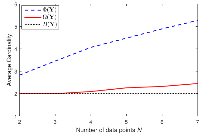
Figure 2: Average cardinality of fixed-point set $\Phi(\mathbf{Y})$ [19, 20], bit-flipping convergence set $\Omega(\mathbf{Y})$, and set of optimal points $B(\mathbf{Y})$ versus number of data points $N$ ($d=2$).

For illustration, in Fig. 2, we demonstrate experimentally the relationship between the cardinalities of $\Phi(\mathbf{Y})$, $\Omega(\mathbf{Y})$, and $B(\mathbf{Y})$. We generate $1000$ independent instances of a full-rank data matrix $\mathbf{Y}\in\mathbb{R}^{(d=2)\times N}$ for $N=2,3,\ldots,7$, with each element of $\mathbf{Y}$ drawn independently from the Gaussian $\mathcal{N}(0,1)$ distribution. Then, we plot the average observed cardinality of $\Phi(\mathbf{Y})$, $\Omega(\mathbf{Y})$, and $B(\mathbf{Y})$ versus the number of data points $N$. We see that as $N$ increases $\Omega(\mathbf{Y})$ remains a tight super-set of $B(\mathbf{Y})$, while the cardinality of $\Phi(\mathbf{Y})$ (number of possible converging points of the FP iterations) increases at a far higher rate. Fig. 2 offers insight why the proposed BF iterations are expected to return the optimal solution to (4) much more often than the FP iterations of [19, 20, 21].

Performance Bounds

The performance attained by $\mathbf{q}_{\mathrm{bf}}$ is formally lower bounded by Proposition 5 whose proof is given in the Appendix.

Proposition 5.

The performance of $\mathbf{q}_{\mathrm{bf}}$ in the metric of (1), calculated upon any initialization, is lower bounded by $\left\|\mathbf{X}^{\top}\mathbf{q}_{\mathrm{bf}}\right\|_{1}\geq\left\|\mathbf{X}\right\|_{F}.$

Moreover, for the optimal L1-PC $\mathbf{q}_{L1}$

$$\left\|\mathbf{X}^{\top}\mathbf{q}_{L1}\right\|_{1} =\left\|\mathbf{X}\mathbf{b}_{\mathrm{opt}}\right\|_{2}=\sqrt{N}\underset{\mathbf{z}\in\{\pm\frac{1}{\sqrt{N}}\}^{N}}{\mathrm{max}}\left\|\mathbf{X}\mathbf{z}\right\|_{2}\leq\sqrt{N}\underset{\mathbf{z}\in\mathbb{R}^{N};\leavevmode\nobreak\ \left\|\mathbf{z}\right\|_{2}=1}{\mathrm{max}}\left\|\mathbf{X}\mathbf{z}\right\|_{2}=\sqrt{N}\sigma_{\max}$$ (26)

where $\sigma_{\max}$ is the maximum singular value of the data matrix $\mathbf{X}$. Then, the loss with respect to the L1-PCA metric in (1) experienced by $\mathbf{q}_{\mathrm{bf}}$ is bounded by

$$\left\|\mathbf{X}^{\top}\mathbf{q}_{L1}\right\|_{1}-\left\|\mathbf{X}^{\top}\mathbf{q}_{\mathrm{bf}}\right\|_{1}\leq\sqrt{N}\sigma_{\max}-\left\|\mathbf{X}\right\|_{F}.$$ (27)

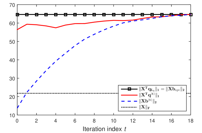
Figure 3: Binary quadratic metric $\|\mathbf{X}^{\top}\mathbf{b}^{(t)}\|_{2}$ and L1-PCA metric $\|\mathbf{X}^{\top}\mathbf{q}^{(t)}\|_{1}$ per iteration. We plot along the upper bound line $\|\mathbf{X}^{\top}\mathbf{q}_{L1}\|_{1}=\|\mathbf{X}\mathbf{b}_{\mathrm{opt}}\|_{2}$ and lower bound line $\|\mathbf{X}\|_{F}$ of Proposition 5.

In Fig. 3, we execute the proposed BF iterations on an arbitrary data matrix $\mathbf{X}\in\mathbb{R}^{(d=4)\times(N=32)}$ (elements drawn independently from $\mathcal{N}(0,1)$) and plot the binary quadratic metric $\|\mathbf{X}\mathbf{b}^{(t)}\|_{2}$ and L1-PCA metric $\|\mathbf{X}^{\top}\mathbf{q}^{(t)}\|_{1}$ per iteration $t$. For reference, we also plot the optimal line $\|\mathbf{X}^{\top}\mathbf{q}_{L1}\|_{1}=\|\mathbf{X}\mathbf{b}_{\mathrm{opt}}\|_{2}$ and lower bound $\|\mathbf{X}\|_{F}$. Fig. 3 offers a vivid numerical illustration of Proposition 5 and eq. (27).

Initialization

Next, we consider initializations that may both expedite convergence and offer superior L1-PC approximations. In the trivial $d=1$ case, $\mathbf{Y}=\sigma\mathbf{v}^{\top}$ for some $\sigma\in\mathbb{R}_{+}$ and $\mathbf{v}\in\mathbb{R}^{N\times 1}$, $\left\|\mathbf{v}\right\|_{2}=1$, and $\mathbf{b}_{\mathrm{opt}}={\arg\max}_{{\mathbf{b}\in\mathbb{\{}\pm 1\}^{N}}}\left\|\mathbf{Y}\mathbf{b}\right\|_{2}^{2}={\arg\max}_{{\mathbf{b}\in\mathbb{\{}\pm 1\}^{N}}}|\mathbf{v}^{\top}\mathbf{b}|_{2}^{2}=\pm\mathrm{sgn}(\mathbf{v})$. Motivated by this special case, we initialize the BF iterations to the sign of the right singular vector of $\mathbf{Y}$ that corresponds to the highest singular value. We call this initialization choice sv-sign initialization. Evidently, by the definition of $\mathbf{Y}$ in (10),

$$\mathbf{b}^{(1)}=\mathrm{sgn}([\mathbf{Y}^{\top}]_{:,1}).$$ (28)

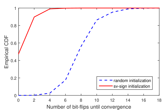
Figure 4: Empirical CDF of number of bit-flips needed until convergence for sv-sign and random initialization ($D=3$, $N=20$, $1000$ experiments).

Experimental studies that compare the efficiency of the proposed sv-sign initialization with that of equiprobable random initializations ($\mathbf{b}^{(1)}$ takes any value in $\{\pm 1\}^{N}$ with probability $2^{-N}$) show that sv-sign initialization not only leads to superior L1-PC approximations with respect to (1), but also reduces significantly the actual execution time of the proposed algorithm by reducing the number of bit-flips needed for convergence. As an illustration, we generate $1000$ realizations of the data matrix $\mathbf{X}\in\mathbb{R}^{3\times 20}$ with entries drawn independently from $\mathcal{N}(0,1)$. On each realization we run bit-flipping iterations with both sv-sign and equiprobable binary initialization. We observe that $81.6\%$ of the time the L1-PC obtained with sv-sign initialization attains value in the metric of (1) greater than or equal to L1-PC obtained by random initialization. Also, in Fig. 4 we plot the empirical CDF of the number of bit-flips needed until convergence for the two initializations. We observe that $50\%$ of the time sv-sign initialization is already in the convergence set $\Omega(\mathbf{X})$ and no bit-flips take place. Moreover, with sv-sign initialization no more than $6$ bit-flips are needed for convergence with empirical probability $1$. On the contrary, random initialization may need with non-zero probability up to $16$ bit-flips for convergence.

Complexity Analysis

Prior to bit-flipping iterations, L1-BF calculates $\mathbf{Y}$ in (10) and chooses the initial binary vector $\mathbf{b}^{(1)}$ with complexity $\mathcal{O}(ND\mathrm{min}\{N,D\})$ (SVD). Then, the algorithm calculates and stores the correlation matrix $\mathbf{Y}^{\top}\mathbf{Y}\in\mathbb{R}^{N\times N}$ with complexity $\mathcal{O}(N^{2}d)$ and, given $\mathbf{b}^{(1)}$ and $\mathbf{Y}^{\top}\mathbf{Y}$, evaluates by (III.A) the initial contribution factors $\alpha\left(\mathbf{b}^{(1)},{n}\right)$ for all $n\in\{1,2,\ldots,N\}$ with cost $\mathcal{O}(N^{2})$. Therefore, initialization has total cost $\mathcal{O}(ND\mathrm{min}\{N,D\}+N^{2}(d+1))$. At iteration $t\geq 1$, finding $n$ by (20) costs $\mathcal{O}(N)$. In case $\alpha\left(\mathbf{b}^{(t)},{n}\right)>0$, repetition of the maximization over the entire index set $\{1,2,\ldots,N\}$ costs an additional $\mathcal{O}(N)$. Therefore, each bit flip costs $\mathcal{O}(N)$. Denoting by $M$ the number of bit flips until the termination criterion is met, we find that the computational cost for calculating $\mathbf{b}_{\mathrm{bf}}$ is $\mathcal{O}(ND\mathrm{min}\{N,D\}+N^{2}(d+1)+MN)$.

Finally, taking into account the computation of $\mathbf{q}_{\mathrm{bf}}$ from $\mathbf{b}_{\mathrm{bf}}$, the proposed L1-BF algorithm costs $\mathcal{O}(ND$ $\mathrm{min}\{N,D\}$ $+N^{2}(d+1)+(M+D)N)$. According to our experiments, $M$ is with empirical probability $1$ upper bounded by $N$; that is, no more than $N$ bits need to be flipped to reach $\mathbf{b}_{\mathrm{bf}}$. Therefore, the total complexity of the proposed algorithm becomes $\mathcal{O}(ND\mathrm{min}\{N,D\}+N^{2}(d+2)+ND)$. Keeping only the dominant complexity terms, L1-BF has complexity $\mathcal{O}(ND\mathrm{min}\{N,D\}+N^{2}d)$, i.e. quadratic in $N$ and either linear, or quadratic in $D$ (depending on the cost of the initial SVD). Thus, the proposed L1-BF algorithm has cost comparable to that of standard PCA (SVD). A summary of the calculated complexity is provided in Table I.

Multiple Initializations

For further L1-PCA metric improvement, we may also run BF on $L$ distinct initialization points, $\mathbf{b}^{(1)}_{1}=\mathrm{sgn}([\mathbf{Y}^{\top}]_{:,1})$ and $\mathbf{b}^{(1)}_{l}=\mathrm{sgn}(\mathbf{Y}^{\top}\mathbf{a}_{l})$, with $\mathbf{a}_{l}\sim\mathcal{N}(\mathbf{0}_{d},\mathbf{I}_{d})$, $l=2,\ldots,L$, to obtain $L$ corresponding convergence points $\mathbf{b}_{\mathrm{bf},1},\mathbf{b}_{\mathrm{bf},2},\ldots,\mathbf{b}_{\mathrm{bf},L}$. Then, if $\mathbf{q}_{\mathrm{bf},l}=\mathbf{X}\mathbf{b}_{\mathrm{bf},l}\left\|\mathbf{X}\mathbf{b}_{\mathrm{bf},l}\right\|_{2}^{-1}$, $l=1,\ldots,N$, we return $\mathbf{q}_{\mathrm{bf}}^{(L)}={\mathrm{argmax}}_{\mathbf{q}\in\{\mathbf{q}_{\mathrm{bf},1},\ldots,\mathbf{q}_{\mathrm{bf},L}\}}\left\|\mathbf{X}^{\top}\mathbf{q}\right\|_{1}.$ Certainly, multiple initializations will increase the complexity of the algorithm by a constant factor $L$.

III.B Calculation of $K>1$ L1-Principal Components

In contrast to L2-PCA, L1-PCA in (1) is not a scalable problem [2]. Therefore, successive-nullspace-projection approaches [19, 22] fail to return optimal L1-PC bases. Optimal L1-PCA demands joint computation of all $K$ principal components of $\mathbf{Y}$, a procedure that increases exponentially in $K$ the computational complexity of optimal algorithms. In this section, we generalize the BF algorithm presented in Section III.A to calculate $K>1$ L1-PCs of any given data matrix $\mathbf{X}\in\mathbb{R}^{D\times N}$ of rank $d\geq K$.

Given the reduced-size, full-row-rank data matrix $\mathbf{Y}\in\mathbb{R}^{d\times N}$ (see Proposition 1), the proposed algorithm first attempts to approximate the solution to (12) $\mathbf{B}_{\mathrm{opt}}$. To do so, it begins from an initial matrix $\mathbf{B}^{(1)}$ and employs bit-flipping iterations to reach an approximation to $\mathbf{B}_{\mathrm{opt}}$, say $\mathbf{B}_{\mathrm{bf}}$. Finally, per (29) the algorithm returns

$$\mathbf{Q}_{\mathrm{bf}}=U\left(\mathbf{X}\mathbf{B}_{\mathrm{bf}}\right).$$ (29)

Evidently, if $\mathbf{B}_{\mathrm{bf}}$ is an exact solution to (2), then $\mathbf{Q}_{\mathrm{bf}}$ is an exact solution to the L1-PCA problem in (1).

Calculation of $\mathbf{B}_{\mathrm{bf}}$ via Bit-flipping Iterations

The algorithm initializes at a binary matrix ${\mathbf{B}^{(1)}}$ and employs BF iterations to generate a sequence of binary matrices $\mathbf{B}^{(t)}$, $t=2,3,\ldots$, such that each matrix $\mathbf{B}^{(t)}$ attains the highest possible value in the maximization metric of (12) given that it differs from $\mathbf{B}^{(t-1)}$ in exactly one entry. Similar to the $K=1$ case, the indices of bits that have not been flipped throughout the iterations are kept in a memory index-set $\mathcal{L}$ initialized at $\{1,2,\ldots,NK\}$ (the $(n,k)$th bit of the binary matrix argument in (12) has corresponding single-integer index $(k-1)N+n\in\{1,2,\ldots,NK\}$).

Mathematically, at the $t$th iteration step, $t\geq 1$, we search for the single bit in the current binary argument $\mathbf{B}^{(t)}$ whose index is not in $\mathcal{L}$ and its flipping increases the nuclear-norm metric $\|\mathbf{Y}\mathbf{B}^{(t)}\|_{*}$ the most. We notice that if we flip the $(n,k)$th bit of $\mathbf{B}^{(t)}$ setting $\mathbf{B}^{(t+1)}=\mathbf{B}^{(t)}-2B_{n,k}^{(t)}\mathbf{e}_{n,N}\mathbf{e}_{k,K}^{\top}$, then

$$\mathbf{Y}\mathbf{B}^{(t+1)}=\mathbf{Y}\mathbf{B}^{(t)}-2B_{n,k}^{(t)}\mathbf{y}_{n}\mathbf{e}_{k,K}^{\top}.$$ (30)

Therefore, at the $t$th iteration step, the algorithm obtains the index pair

$$(n,k)=\underset{\begin{smallmatrix}(m,l)\in\{1,2,\ldots,N\}\times\{1,2,\ldots,K\}\\ (l-1)N+m\in\mathcal{L}\end{smallmatrix}}{\mathrm{argmax}}\left\|\mathbf{Y}\mathbf{B}^{(t)}-2B_{m,l}^{(t)}\mathbf{y}_{m}\mathbf{e}_{l,K}^{\top}\right\|_{*}.$$ (31)

If $\left\|\mathbf{Y}\mathbf{B}^{(t)}-2B_{n,k}^{(t)}\mathbf{y}_{n}\mathbf{e}_{k,K}^{\top}\right\|_{*}>\left\|\mathbf{Y}\mathbf{B}^{(t)}\right\|_{*}$, the algorithm flips $B_{n,k}^{(t)}$ setting $\mathbf{B}^{(t+1)}=\mathbf{B}^{(t)}-2B_{n,k}^{(t)}\mathbf{e}_{n,N}\mathbf{e}_{k,K}^{\top}$ and updates $\mathcal{L}$ to $\mathcal{L}\setminus\{(k-1)N+n\}$. If, otherwise, $\left\|\mathbf{Y}\mathbf{B}^{(t)}-2B_{n,k}^{(t)}\mathbf{y}_{n}\mathbf{e}_{k,K}^{\top}\right\|_{*}\leq\left\|\mathbf{Y}\mathbf{B}^{(t)}\right\|_{*}$, the algorithm obtains a new solution $(n,k)$ to (31) after resetting $\mathcal{L}$ to $\{1,2,\ldots,NK\}$. If now, for this new pair $(n,k)$, $\left\|\mathbf{Y}\mathbf{B}^{(t)}-2B_{n,k}^{(t)}\mathbf{y}_{n}\mathbf{e}_{k,K}^{\top}\right\|_{*}>\left\|\mathbf{Y}\mathbf{B}^{(t)}\right\|_{*}$, the algorithm sets $\mathbf{B}^{(t+1)}=\mathbf{B}^{(t)}-2B_{n,k}^{(t)}\mathbf{e}_{n,N}\mathbf{e}_{k,K}^{\top}$ and updates $\mathcal{L}=\mathcal{L}\setminus\{(k-1)N+n\}$. Otherwise, the iterations terminate and the algorithm returns $\mathbf{B}_{\mathrm{bf}}=\mathbf{B}^{(t)}$ and $\mathbf{Q}_{\mathrm{bf}}=\hat{\mathbf{U}}\hat{\mathbf{V}}^{\top}$, where $\mathbf{X}\mathbf{B}_{\mathrm{bf}}\overset{\mathrm{SVD}}{=}\hat{\mathbf{U}}_{D\times K}\hat{\mathbf{\Sigma}}_{K\times K}\hat{\mathbf{V}}_{K\times K}^{\top}$.

We note that to solve (31) exhaustively, one has to calculate $\left\|\mathbf{Y}\mathbf{B}^{(t)}-2B_{m,l}^{(t)}\mathbf{y}_{m}\mathbf{e}_{l,K}^{\top}\right\|_{*}$ for all $(m,l)\in\{1,2,\ldots,N\}\times\{1,2,\ldots,K\}$ such that $(l-1)N+m\in\mathcal{L}$. In worst case, $\mathcal{L}=\{1,2,\ldots,NK\}$ and this demands $NK$ independent singular-value/nuclear-norm calculations. A simplistic, but computationally inefficient, approach would be perform an SVD on $\mathbf{Y}\mathbf{B}^{(t)}-2B_{m,l}^{(t)}\mathbf{y}_{m}\mathbf{e}_{l,K}^{\top}$ from scratch with cost $\mathcal{O}(dK^{2})$. This would yield a worst case total cost of $\mathcal{O}(NdK^{3})$ to find $(n,k)$ in (31). Below, we present an alternative method to solve (31) with cost $\mathcal{O}(dK^{2}+N(K^{3}+dK))$.

Reduced-cost Nuclear-norm Evaluations for Optimal Bit-flipping

At the beginning of the $t$th iteration step, we perform the singular-value decomposition

$$\mathbf{Y}\mathbf{B}^{(t)}\overset{\mathrm{SVD}}{=}\mathbf{U}_{d\times K}^{(t)}\mathbf{S}_{K\times K}^{(t)}\mathbf{V}_{K\times K}^{{(t)}^{\top}}$$ (32)

with cost $\mathcal{O}(dK^{2})$. Then, for any $(m,l)\in\{1,2,\ldots,N\}\times\{1,2,\ldots,K\}$, the singular values of $\mathbf{Y}\mathbf{B}^{(t)}-2B_{m,l}^{(t)}\mathbf{y}_{m}\mathbf{e}_{l,K}^{\top}$ are the square roots of the eigenvalues of $(\mathbf{Y}\mathbf{B}^{(t)}-2B_{m,l}^{(t)}\mathbf{y}_{m}\mathbf{e}_{l,K}^{\top})^{\top}(\mathbf{Y}\mathbf{B}^{(t)}-2B_{m,l}^{(t)}\mathbf{y}_{m}\mathbf{e}_{l,K}^{\top})$ (found with constant cost), which due to rotation invariance are equal to the eigenvalues of $\mathbf{A}=\mathbf{V}^{{(t)}^{\top}}(\mathbf{Y}\mathbf{B}^{(t)}-2B_{m,l}^{(t)}\mathbf{y}_{m}\mathbf{e}_{l,K}^{\top})^{\top}(\mathbf{Y}\mathbf{B}^{(t)}-2B_{m,l}^{(t)}\mathbf{y}_{m}\mathbf{e}_{l,K}^{\top})\mathbf{V}^{(t)}.$ Defining $\mathbf{W}=[[\mathbf{V}^{(t)}]_{l,:}^{\top},-2B_{m,l}^{(t)}\mathbf{S}^{{(t)}^{\top}}\mathbf{U}^{{(t)}^{\top}}\mathbf{y}_{m}]\in\mathbb{R}^{K\times 2}$ and the eigenvalue decomposition (EVD) $\mathbf{Q}\mathbf{D}\mathbf{Q}^{\top}\overset{\text{EVD}}{=}\|\mathbf{y}_{m}\|_{2}^{2}\mathbf{e}_{1,2}\mathbf{e}_{1,2}^{\top}+[\mathbf{e}_{2,2},\mathbf{e}_{1,2}]$ where $\mathbf{D}=\mathrm{diag}([d_{1},\leavevmode\nobreak\ d_{2}]^{\top})$, it is easy to show that

$$\mathbf{A}=\mathbf{S}^{{(t)}^{\top}}\mathbf{S}^{{(t)}}+d_{1}\mathbf{W}\mathbf{q}_{1}(\mathbf{W}\mathbf{q}_{1})^{\top}+d_{2}\mathbf{W}\mathbf{q}_{2}(\mathbf{W}\mathbf{q}_{2})^{\top}.$$ (33)

Consider now the eigenvalue decomposition

$$\mathbf{Z}_{K\times K}\mathbf{P}\mathbf{Z}^{\top}\overset{\mathrm{EVD}}{=}\mathbf{S}^{{(t)}^{\top}}\mathbf{S}^{{(t)}}+d_{1}\mathbf{W}\mathbf{q}_{1}(\mathbf{W}\mathbf{q}_{1})^{\top}.$$ (34)

Then, again by eigenvalue permutation invariance, the singular values of $\mathbf{Y}\mathbf{B}^{(t)}-2B_{m,l}^{(t)}\mathbf{y}_{m}\mathbf{e}_{l,K}^{\top}$ are equal to the square roots of the eigenvalues of

$$\mathbf{Z}^{\top}\mathbf{A}\mathbf{Z}=\mathbf{P}+d_{2}\mathbf{Z}^{\top}\mathbf{W}\mathbf{q}_{2}(\mathbf{Z}^{\top}\mathbf{W}\mathbf{q}_{2})^{\top}.$$ (35)

Notice that matrix ${\mathbf{S}^{(t)}}^{\top}{\mathbf{U}^{(t)}}^{\top}$ needed for the calculation of $\mathbf{W}$ is constant for all candidate-bit evaluations of the $t$th iteration and, given the SVD of $\mathbf{Y}\mathbf{B}^{(t)}$, can be found with cost $\mathcal{O}(K^{2})$. Thus, this computational cost is absorbed in the SVD of $\mathbf{Y}\mathbf{B}^{(t)}$. Then, for bit-flip examination of all $K$ bits of the $m$th row of $\mathbf{B}^{(t)}$ it suffices to calculate the quantities $\mathbf{Q}$, $\mathbf{d}$, and ${\mathbf{S}^{(t)}}^{\top}{\mathbf{U}^{(t)}}^{\top}\mathbf{y}_{m}$, appearing in $\mathbf{S}^{{(t)}^{\top}}\mathbf{S}^{{(t)}}+d_{1}\mathbf{W}\mathbf{q}_{1}(\mathbf{W}\mathbf{q}_{1})^{\top}$ and $d_{2}\mathbf{W}\mathbf{q}_{2}$, just once with cost $\mathcal{O}(dK)$. Employing the algorithm proposed in [40] for the EVD of a diagonal positive semidefinite matrix perturbated by a rank-1 symmetric matrix, EVD of $\mathbf{S}^{{(t)}^{\top}}\mathbf{S}^{{(t)}}+d_{1}\mathbf{W}\mathbf{q}_{1}(\mathbf{W}\mathbf{q}_{1})^{\top}$ (i.e., calculation of $\mathbf{Z}$ and $\mathbf{P}$) costs $\mathcal{O}(K^{2})$. Then, defining $d_{2}\mathbf{Z}^{\top}\mathbf{W}\mathbf{q}_{2}(\mathbf{Z}^{\top}\mathbf{W}\mathbf{q}_{2})^{\top}$ and finding the eigenvalues of $\mathbf{P}+d_{2}\mathbf{Z}^{\top}\mathbf{W}\mathbf{q}_{2}(\mathbf{Z}^{\top}\mathbf{W}\mathbf{q}_{2})^{\top}$ (again per [40]) costs an additional $\mathcal{O}(K^{2})$. Thus, including the initial SVD, the total cost for bit-flipping examination of all bits in $\mathbf{B}^{(t)}$ (worst case scenario) is $\mathcal{O}(dK^{2})+N\mathcal{O}(dK)+NK\mathcal{O}(K^{2})\equiv\mathcal{O}(dK^{2}+N(K^{3}+dK)).$

Termination Guarantee

Similarly to the $K=1$ case, the termination condition

$$\left\|\mathbf{Y}\mathbf{B}^{(t)}-2B_{m,l}^{(t)}\mathbf{y}_{m}\mathbf{e}_{l,K}^{\top}\right\|_{*}\leq\left\|\mathbf{Y}\mathbf{B}^{(t)}\right\|_{*}\leavevmode\nobreak\ \leavevmode\nobreak\ \forall(m,l)\in\{1,2,\ldots,N\}\times\{1,2,\ldots,K\}$$ (36)

is guaranteed to be met after a finite number of iterations because (i) binary nuclear-norm maximization in (2) has finite upper bound and (ii) at every step of the BF iterations the nuclear-norm value increases.

Initialization

Generalizing the initialization idea for the $K=1$ case, we choose $\mathbf{B}^{(1)}=\mathrm{sgn}([\mathbf{Y}^{\top}]_{:,1})\mathbf{1}_{K}^{\top}$ where $\mathbf{1}_{K}$ is the all-one vector of length $K$. Again, our motivation here lies in the fact that for $d=1$ and any $K$, $\mathbf{B}_{\mathrm{opt}}=\mathrm{sgn}(\mathbf{v}_{\mathrm{opt}})\mathbf{1}_{K}^{\top}$. For this particular initialization, $\left\|\mathbf{Y}\mathbf{B}^{(1)}\right\|_{*}=K\left\|\mathbf{Y}\mathrm{sgn}([\mathbf{Y}^{\top}]_{:,1})\right\|_{2}.$ Pseudocode of the proposed L1-BF algorithm for $K\geq 1$ is offered in Fig. 5. Of course, for $K=1$ the L1-PCs generated by the algorithms of Fig. 1 and Fig. 5 coincide.

Complexity Analysis

Before the BF iterations, the algorithm expends $\mathcal{O}(ND\mathrm{min}\{N,D\})$ to calculate $\mathbf{Y}\in\mathbb{R}^{d\times N}$ through SVD of $\mathbf{X}\in\mathbb{R}^{D\times N}$. By the same SVD, we calculate also the initial binary matrix. Then, for the proposed initialization $\mathbf{Y}\mathbf{B}^{(1)}$ and $\left\|\mathbf{Y}\mathbf{B}^{(1)}\right\|_{*}$ are calculated in the beginning of the first iteration with complexity $\mathcal{O}(NdK)$. To find a solution to (31), we incur worst case cost $\mathcal{O}(dK^{2}+N(K^{3}+dK))$. Setting the maximum number of BF iterations run by the algorithm to $NK$, the total complexity to calculate $\mathbf{B}_{\mathrm{bf}}$ is in worst case $\mathcal{O}(ND\mathrm{min}\{N,D\}+NdK^{3}+N^{2}(K^{4}+dK^{2}))$. Then, to calculate $\mathbf{Q}_{\mathrm{bf}}$ from $\mathbf{B}_{\mathrm{bf}}$ costs an additional $\mathcal{O}(ND\mathrm{min}\{N,D\}+NDK)$. Therefore, the total complexity of the proposed algorithm is $\mathcal{O}(ND\mathrm{min}\{N,D\}+N^{2}(K^{4}+dK^{2})+NdK^{3})$; that is, quadratic complexity in $N$ and at most quadratic complexity in $D$. Notice that for $K=1$ the asymptotic complexity of the algorithm becomes $\mathcal{O}(ND\mathrm{min}(N,D)+N^{2}d)$, i.e. equal to that of the algorithmic operations of Fig. 1. A summary of the calculated complexity is provided in Table II.

Multiple Initializations

Similar to the $K=1$ case, we can further increase performance of the proposed L1-PCA scheme by running BF iterations on $L$ distinct initialization matrices $\mathbf{B}^{(1)}_{1},\mathbf{B}^{(1)}_{2},\ldots,\mathbf{B}^{(1)}_{L}$. We choose $\mathbf{B}^{(1)}_{1}=\mathrm{sgn}([\mathbf{Y}^{\top}]_{:,1})\mathbf{1}_{K}^{\top}$ (sv-sign initialization) and for $l\in\{2,3,\ldots,L\}$ we initialize randomly to $\mathbf{B}^{(1)}_{l}=\mathrm{sgn}(\mathbf{a}_{l})\mathbf{1}_{K}^{\top}$, $\mathbf{a}_{l}\sim\mathcal{N}(\mathbf{0}_{N},\mathbf{I}_{N})$, to obtain the $L$ corresponding convergence points $\mathbf{B}_{\mathrm{bf},1},\mathbf{B}_{\mathrm{bf},2},\ldots,\mathbf{B}_{\mathrm{bf},L}$ and, through (29), the associated L1-PC bases $\mathbf{Q}_{\mathrm{bf},1},\mathbf{Q}_{\mathrm{bf},2},\ldots,\mathbf{Q}_{\mathrm{bf},L}$. Then, we return $\mathbf{Q}_{\mathrm{bf}}^{(L)}={\mathrm{argmax}}_{\mathbf{Q}\in\{\mathbf{Q}_{\mathrm{bf},1},\mathbf{Q}_{\mathrm{bf},2},\ldots,\mathbf{Q}_{\mathrm{bf},L}\}}\left\|\mathbf{X}^{\top}\mathbf{Q}\right\|_{1}.$

IV Experimental Studies

IV.A Comparison of L1-BF with Current State-of-the-art Algorithms

We first compare the performance of L1-BF with that of algorithms proposed in [19, 21, 22]. In our experiment, we generate $1000$ arbitrary matrices of size $(D=d=4)\times(N=16)$ with entries drawn independently from $\mathcal{N}(0,1)$ and calculate the primary ($K=1$) L1-PC by L1-BF iterations ($L=1$ initialization), the fixed-point algorithm of [19, 21] ($L=1$ initialization), and the SDP approach in [22] ($L=1$ Gaussian randomization). We measure the performance degradation experienced by a unit-length vector $\mathbf{q}$ on the metric of (1) by

$$\Delta(\mathbf{q};\mathbf{X})=\frac{\|\mathbf{X}^{\top}\mathbf{q}_{L1}\|_{1}-\|\mathbf{X}^{\top}\mathbf{q}\|_{1}}{\|\mathbf{X}^{\top}\mathbf{q}_{L1}\|_{1}}$$ (37)

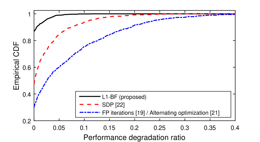
(a)

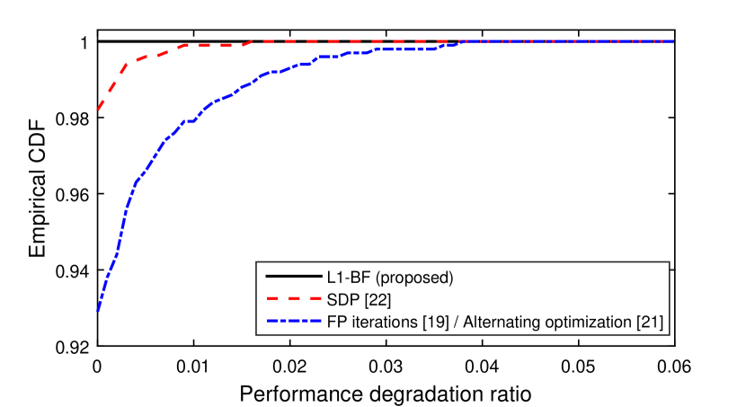
(b)

Figure 6: Empirical CDF of $\Delta(\mathbf{q}_{\mathrm{bf}};\mathbf{X})$, $\Delta(\mathbf{q}_{\mathrm{fp}};\mathbf{X})$, and $\Delta(\mathbf{q}_{\mathrm{sdp}};\mathbf{X})$ ($D=4$, $N=16$) for (a) $L=1$ and (b) $L=N=16$ initializations.

and in Fig. 6(a) we plot the empirical cumulative distribution function (CDF) of $\Delta(\mathbf{q}_{\mathrm{bf}};\mathbf{X})$, $\Delta(\mathbf{q}_{\mathrm{fp}};\mathbf{X})$, and $\Delta(\mathbf{q}_{\mathrm{sdp}};\mathbf{X})$. We observe that $86\%$ of the time, L1-BF returns the exact, optimal L1-PC of $\mathbf{X}$. In addition, the performance degradation attained by the proposed algorithm is, with empirical probability $1$, less than $0.09$. On the other hand, FP iterations [19, 21] and SDP [22] attain optimal performance, with empirical probabilities $0.3$ and $0.5$, respectively. The performance degradation for FP [19, 21] and SDP [22] can be as much as $0.25$ and $0.55$, respectively.

We repeat the same experiment after increasing the number of initializations for the proposed algorithm and the FP [19, 21] to $L=N=16$ and the number of Gaussian randomizations in SDP [22] to $L=N=16$. In Fig. 6(b), we plot the corresponding empirical CDFs of $\Delta(\mathbf{q}_{\mathrm{bf}};\mathbf{X})$, $\Delta(\mathbf{q}_{\mathrm{fp}};\mathbf{X})$, and $\Delta(\mathbf{q}_{\mathrm{sdp}};\mathbf{X})$. L1-BF outperforms the two counterparts, returning the exact L1-PC with empirical probability $1$.

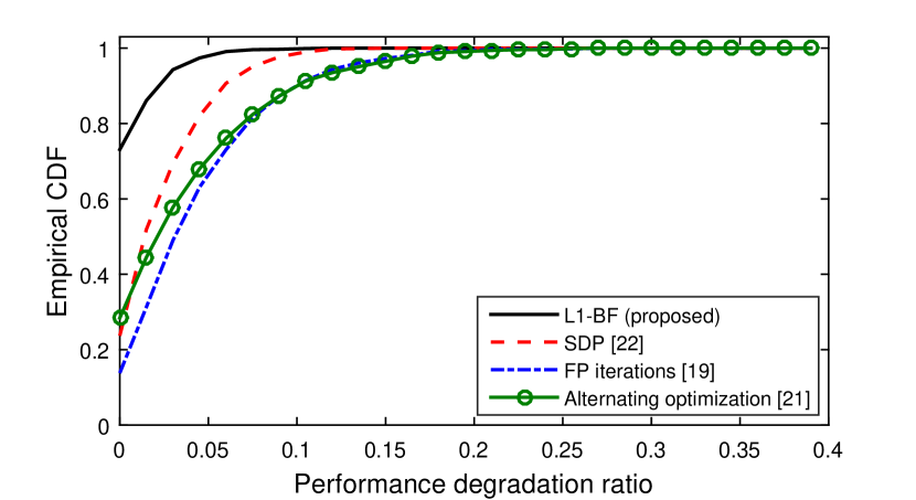
(a)

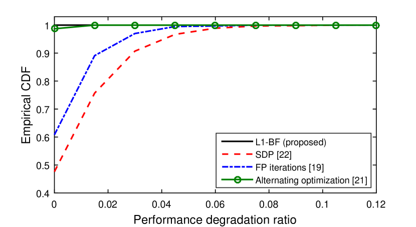
(b)

Figure 7: Empirical CDF of $\Delta(\mathbf{Q}_{\mathrm{ao}};\mathbf{X})$, $\Delta(\mathbf{Q}_{\mathrm{fp}};\mathbf{X})$, $\Delta(\mathbf{Q}_{\mathrm{sdp}};\mathbf{X})$, and $\Delta(\mathbf{Q}_{\mathrm{bf}};\mathbf{X})$ for (a) $L=1$ and (b) $L=NK=16$ initializations.

Next, we examine the performance of the four algorithms (FP iterations with successive nullspace projections [19], alternating optimization [21], and SDP with successive nullspace projections [22], and proposed BF iterations) when $K=2$ L1-PCs are sought. We generate $1000$ arbitrary data matrices of size $(D=3)\times(N=8)$ (all entries drawn independently from $\mathcal{N}(0,1)$) and plot in Fig. 7(a) the empirical CDF of the corresponding performance degradation ratios, $\Delta(\mathbf{Q}_{\mathrm{fp}};\mathbf{X})$, $\Delta(\mathbf{Q}_{\mathrm{ao}};\mathbf{X})$, $\Delta(\mathbf{Q}_{\mathrm{sdp}};\mathbf{X})$, and $\Delta(\mathbf{Q}_{\mathrm{bf}};\mathbf{X})$. All iterative methods are run on a single initialization point (one Gaussian-randomization instance for SDP). We observe that $83\%$ of the time, L1-BF returns the exact, optimal L1-PCs of $\mathbf{X}$. The performance degradation attained by the proposed PCs is, with empirical probability $1$, less than $0.09$. On the other hand, the PCs calculated by [21, 19, 22] attain optimal performance, with empirical probabilities of above $0.31$, $0.05$, and $0.1$, respectively, while the performance degradation for the algorithms in [21, 19] and [22] can be as much as $30\%$. Evidently, the nullspace projections of [19, 22] that “violate” the non-scalability principle of the L1-PCA problem, have significant impact on their performance. Next, we repeat the above experiment with $L=NK=16$ initializations ($L=16$ Gaussian-randomization instances for SDP). In Fig. 7(b), we plot the new performance degradation ratios for the four algorithms. This time, the proposed method returns the exact/optimal L1-PCs of $\mathbf{X}$ with probability $1$. High, but inferior, performance is also attained by the iterative algorithm of [21]. On the other hand, the algorithms in [19, 22] that follow the greedy approach of solving a sequence of nullspace-projected $K=1$ problem instances experience performance degradation values similar to those of Fig. 7(a).

IV.B Line-fitting Experiment

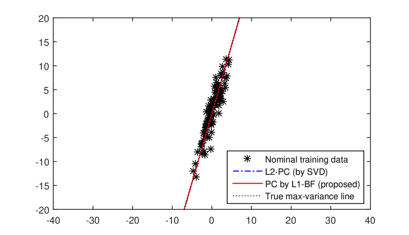
(a)

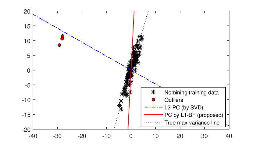
(b)

Figure 8: L2-PC and L1-PC (by L1-BF) trained over (a) the clean data matrix $\mathbf{X}\in\mathbb{R}^{2\times 100}$ ($100$ nominal data points) and (b) the outlier corrupted data matrix $\mathbf{X}_{\mathrm{cor}}\in\mathbb{R}^{2\times 104}$ (same $100$ nominal data points plus $4$ outliers).

For visual evaluation of the outlier resistance of the proposed L1-PCs, we consider $N=100$ $2$-dimensional points drawn from the nominal zero-mean Gaussian distribution $\mathcal{N}\left(\mathbf{0}_{2},\mathbf{R}=\begin{bmatrix}4&10\\ 10&29\end{bmatrix}\right)$ organized in matrix form $\mathbf{X}_{\mathrm{nom}}=[\mathbf{x}_{1},\mathbf{x}_{2},\ldots,\mathbf{x}_{100}]$. We use the nominal data points to extract an estimate of the true maximum-variance/minimum-mean-squared-error subspace (line) of our data distribution by means of L2-PCA (standard SVD method). We do the same by means of L1-PCA through the proposed L1-BF method. In Fig. 8(a), we plot on the $2$-dimensional plain the $100$ training data points in $\mathbf{X}_{\mathrm{nom}}$ and the lines described by $\mathbf{q}_{{L_{2}}}(\mathbf{X}_{\mathrm{nom}})$ and $\mathbf{q}_{\mathrm{bf}}(\mathbf{X}_{\mathrm{nom}})$. For reference, we also plot alongside the true maximum-variance line. All three lines visually coincide, i.e. $\mathbf{q}_{L_{2}}(\mathbf{X}_{\mathrm{nom}})$ and $\mathbf{q}_{\mathrm{bf}}(\mathbf{X}_{\mathrm{nom}})$ are excellent estimates of the true maximum-variance line.

Next, we assume that instead of the clean matrix of nominal training data points $\mathbf{X}_{\mathrm{nom}}$, we are given the outlier-corrupted data matrix $\mathbf{X}_{\mathrm{cor}}=[\mathbf{X}_{\mathrm{nom}},\mathbf{O}]\in\mathbb{R}^{2\times 104}$, for estimating $\mathbf{q}_{\mathrm{opt}}$. Here, in addition to the previous $100$ nominal data points in $\mathbf{X}_{\mathrm{nom}}$, $\mathbf{X}_{\mathrm{cor}}$ also contains the $4$ outliers in $\mathbf{O}=[\mathbf{o}_{1},\mathbf{o}_{2},\mathbf{o}_{3},\mathbf{o}_{4}]\in\mathbb{R}^{2\times 4}$ as seen in Fig. 8(b) that do not follow the nominal distribution. Similar to our treatment of $\mathbf{X}_{\mathrm{nom}}$, we calculate the L2-PC and L1-PC (by L1-BF) of $\mathbf{X}_{\mathrm{cor}}$, $\mathbf{q}_{L_{2}}(\mathbf{X}_{\mathrm{cor}})$ and $\mathbf{q}_{\mathrm{bf}}(\mathbf{X}_{\mathrm{cor}})$, respectively. In Fig. 8(b) we plot the two lines, against the true maximum-variance line of the nominal data. This time, the lines of $\mathbf{q}_{L_{2}}(\mathbf{X}_{\mathrm{cor}})$ and $\mathbf{q}_{\mathrm{bf}}(\mathbf{X}_{\mathrm{cor}})$ differ significantly. In sharp contrast to L1-PC, the L2-PC of $\mathbf{X}_{\mathrm{cor}}$ is strongly attracted by the four outliers and drifting away from the true maximum-variance line. The outlier-resistance and superior line-fitting performance of the proposed approximate L1-PC in the presence of the faulty data is clearly illustrated.

IV.C Classification of Genomic Data – Prostate Cancer Diagnosis

In this experiment, we conduct subspace-classification of MicroRNA (miRNA) data for prostate cancer diagnosis [41, 42]. Specifically, we operate on the expressions of $D=9$ miRNAs (miR-26a, miR-195, miR-342-3p, miR-126*, miR-425*, miR-34a*, miR-29a*, miR-622, miR-30d) that have been recently considered to be differentially expressed between malignant and normal human prostate tissues [43]. For each of the above miRNAs, we obtain one sample expression from one malignant and one normal prostate tissue from $N=19$ patients (patient indexes per [43]: $1,2,\ldots,10,12,\ldots,20$) of the of the Swedish Watchful Waiting cohort [44]. The miRNA expressions from malignant and normal tissues are organized in $\mathbf{X}_{M}=[\mathbf{x}_{M,1},\mathbf{x}_{M,2},\ldots,\mathbf{x}_{M,N}]\in\mathbb{R}^{D\times N}$ and $\mathbf{X}_{N}=[\mathbf{x}_{N,1},\mathbf{x}_{N,2},\ldots,\mathbf{x}_{N,N}]\in\mathbb{R}^{D\times N}$, respectively. The classification/diagnosis experiment is conducted as follows.

We collect $N_{train}=10$ points from $\mathbf{X}_{M}$ in $\mathbf{X}_{M,tr}=[\mathbf{X}_{M}]_{:,\mathcal{I}_{M}}$ with $\mathcal{I}_{M}\subset\{1,2,\ldots,N\}$ and $|\mathcal{I}_{M}|=N_{train}$, and $N_{train}$ points from $\mathbf{X}_{N}$ in $\mathbf{X}_{N,tr}=[\mathbf{X}_{N}]_{:,\mathcal{I}_{N}}$ with $\mathcal{I}_{N}\subset\{1,2,\ldots,N\}$ and $|\mathcal{I}_{N}|=N_{train}$. Then, we calculate the zero-centered malignant and normal tissue training datasets $\tilde{\mathbf{X}}_{M,tr}={\mathbf{X}}_{M,tr}-\mathbf{m}_{M}\mathbf{1}_{N_{train}}^{\top}$ where $\mathbf{m}_{M}=\frac{1}{N_{train}}{\mathbf{X}}_{M,tr}\mathbf{1}_{N_{train}}$ and $\tilde{\mathbf{X}}_{N,tr}={\mathbf{X}}_{N,tr}-\mathbf{m}_{N}\mathbf{1}_{N_{train}}^{\top}$ where $\mathbf{m}_{N}=\frac{1}{N_{train}}{\mathbf{X}}_{N,tr}\mathbf{1}_{N_{train}}$, respectively. Next, we find $K=3$ L2-PCs or L1-PCs by L1-BF of the zero-centered malignant and normal datasets, $\mathbf{Q}_{M}\in\mathbb{R}^{D\times K}$ and $\mathbf{Q}_{N}\in\mathbb{R}^{D\times K}$, respectively, and conduct subspace-classification [45, 46] of each data-point $\mathbf{x}$ that has not been used for PC training (i.e., every $\mathbf{x}\in\{\mathbf{x}_{M,i}\}_{i\in\mathcal{I}_{M}^{c}}\cup\{\mathbf{x}_{N,i}\}_{i\in\mathcal{I}_{N}^{c}}$ where $\mathcal{I}_{M}^{c}=\{1,2,\ldots,N\}\setminus\mathcal{I}_{M}$ and $\mathcal{I}_{N}^{c}=\{1,2,\ldots,N\}\setminus\mathcal{I}_{N}$) as

$$\|\mathbf{Q}_{M}^{\top}(\mathbf{x}-\mathbf{m}_{M})\|_{2}^{2}\overset{\overset{\text{\footnotesize{malignant}}}{\text{\normalsize{$>$}}}}{\underset{\text{\footnotesize{normal}}}{{<}}}\|\mathbf{Q}_{N}^{\top}(\mathbf{x}-\mathbf{m}_{N})\|_{2}^{2}+\lambda$$ (38)

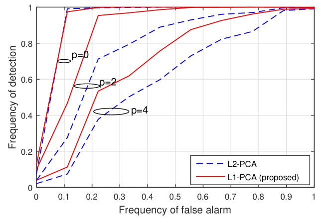
Figure 9: ROC curve of L2-PCA and L1-PCA (L1-BF) malignant tissue detector for $p=0,2,4$ mislabeled points per training dataset ($N=19$, $N_{train}=10$, $D=9$, $K=3$).

where $\lambda$ is the classification/detection bias term. We run the above classification experiment over $2000$ distinct training-dataset configurations and calculate the receiver operating characteristic (ROC) curve of the developed L2-PCA or L1-PCA classifier identifying as “detection” the event of classifying correctly a malignant tissue and as “false alarm” the event of classifying erroneously a normal tissue (Fig. 9, “$p=0$” curves).

Next, we consider the event of training on faulty/mislabeled data. That is, we recalculate the above ROC curves having exchanged $p=2$ or $4$ data points between $\mathbf{X}_{M,tr}$ and $\mathbf{X}_{N,tr}$. In Fig. 9, we plot the ROC curves for the designed L2-PCA and L1-PCA malignant tissue detectors, for $K=3$ and $p=0,2,4$. We observe that for $p=0$ (no mislabeling) the the two classifiers perform almost identically, attaining frequency of detection (FD) close to 1 for frequency of false alarm (FFA) less than 0.15. However, in the event of training data mislabeling, the strong resistance of the proposed L1-PCs against dataset contamination is apparent. The L1-PCA classifier outperforms significantly L2-PCA, for every examined value of $p$. For instance, for $p=2$, L1-PCA achieves FD of $.95$ for FFA $0.23$, while L2-PCA achieves the same FD for FFA $.65$.

V Conclusions

In this work, we presented a novel, near-optimal, bit-flipping based algorithm named L1-BF, to calculate $K$ L1-PCs of any rank-$d$ $D\times N$ data matrix with complexity $\mathcal{O}(ND\mathrm{min}\{N,D\}+N^{2}(K^{4}+dK^{2})+NdK^{3})$. Formal proof of convergence, theoretical analysis of converging points, and detailed asymptotic complexity derivation were carried out. Our numerical experiments show that the proposed algorithm outperforms in the optimization metric all other L1-PCA calculators at cost comparable to L2-PCA. L1-PCA and L2-PCA have almost indistinguishable behavior on clean, nominal data. L1-PCA shows remarkable relative resistance to faulty data contamination. Thus, the proposed algorithm, retaining the robustness of L1-PCA at a cost close to that of L2-PCA, may bridge the gap between outlier resistant and computationally efficient principal-component analysis.

.A Proof of Proposition 5

Since $\mathbf{b}_{\mathrm{bf}}\in\Omega(\mathbf{Y})$, (24) and (11) imply

$$\left\|\mathbf{Y}\mathbf{b}_{\mathrm{bf}}\right\|_{2}^{2} =\sum_{n\in\{1,2,\ldots,N\}}b_{n}\mathbf{y}_{n}^{\top}\mathbf{Y}\mathbf{b}$$

$$\geq\sum_{n\in\{1,2,\ldots,N\}}\left\|\mathbf{y}_{n}\right\|_{2}^{2}=\left\|\mathbf{Y}\right\|_{F}^{2}=\left\|\mathbf{X}\right\|_{F}^{2}.$$ (39)

In addition, by Proposition 4, $\mathbf{b}_{\mathrm{bf}}$ lies in $\Phi(\mathbf{Y})$ as well and satisfies $\mathbf{b}_{\mathrm{bf}}=\mathrm{sgn}(\mathbf{Y}^{\top}\mathbf{Y}\mathbf{b}_{\mathrm{bf}})$. Therefore, for $\mathbf{q}_{\mathrm{bf}}=\mathbf{X}\mathbf{b}_{\mathrm{bf}}\left\|\mathbf{X}\mathbf{b}_{\mathrm{bf}}\right\|_{2}^{-1}$,

$$\left\|\mathbf{X}^{\top}\mathbf{q}_{\mathrm{bf}}\right\|_{1} ={\left\|\mathbf{X}^{\top}\mathbf{X}\mathbf{b}_{\mathrm{bf}}\right\|_{1}}{\left\|\mathbf{X}\mathbf{b}_{\mathrm{bf}}\right\|_{2}^{-1}}$$

$$=\left(\mathrm{sgn}(\mathbf{X}^{\top}\mathbf{X}\mathbf{b}_{\mathrm{bf}})^{\top}\mathbf{X}^{\top}\mathbf{X}\mathbf{b}_{\mathrm{bf}}\right)\left\|\mathbf{X}\mathbf{b}_{\mathrm{bf}}\right\|_{2}^{-1}$$

$$=\left(\mathrm{sgn}(\mathbf{Y}^{\top}\mathbf{Y}\mathbf{b}_{\mathrm{bf}})^{\top}\mathbf{X}^{\top}\mathbf{X}\mathbf{b}_{\mathrm{bf}}\right)\left\|\mathbf{X}\mathbf{b}_{\mathrm{bf}}\right\|_{2}^{-1}$$

$$=\left\|\mathbf{X}\mathbf{b}_{\mathrm{bf}}\right\|_{2}\overset{\eqref{ch2_SBFbound1}}{=}\left\|\mathbf{Y}\mathbf{b}_{\mathrm{bf}}\right\|_{2}\geq\left\|\mathbf{X}\right\|_{F}.$$ (40)

∎

    L1-BF for the calculation of the first L1-norm principal component ($K=1$)   Input: $\mathbf{X}_{D\times N}$
1: $(\mathbf{U},\mathbf{\Sigma},\mathbf{V})\leftarrow\mathrm{csvd}(\mathbf{X})$, $\mathbf{Y}\leftarrow\mathbf{\Sigma}\mathbf{V}^{\top}$ 2: $\mathbf{b}_{\mathrm{bf}}\leftarrow\mathrm{bf}\left(\mathbf{Y}^{\top}\mathbf{Y},\mathrm{sgn}([\mathbf{Y}]_{:,1})\right)$ 3: $\mathbf{q}_{\mathrm{bf}}\leftarrow\mathbf{X}\mathbf{b}_{\mathrm{bf}}/\left\|\mathbf{X}\mathbf{b}_{\mathrm{bf}}\right\|_{2}$
Output: $\mathbf{q}_{\mathrm{bf}}$   Function $\mathrm{bf}(\mathbf{A},\mathbf{b})$   1: $N\leftarrow\mathrm{length(\mathbf{b})}$, $\mathcal{L}\leftarrow\{1,2,\ldots,N\}$ 2: $\alpha_{i}\leftarrow 2b_{i}\sum_{m\neq i}\,b_{m}[\mathbf{A}]_{i,m}\leavevmode\nobreak\ \leavevmode\nobreak\ \forall i\in\{1,2,\ldots,N\}$ 3:        while true (or terminate at $N$ BFs) 4:             $n\leftarrow{\mathrm{argmin}}_{m\in\mathcal{L}}\alpha_{m}$ 5:             if $a_{n}\leq 0$, 6:                  $b_{n}\leftarrow-b_{n}$, $\mathcal{L}\leftarrow\mathcal{L}\setminus\{n\}$ 7:                  $a_{n}\leftarrow-a_{n}$, $\alpha_{i}\leftarrow\alpha_{i}-4b_{i}b_{n}[\mathbf{A}]_{i,n}\leavevmode\nobreak\ \leavevmode\nobreak\ \forall i\neq n$ 8:             elseif $a_{n}>0$ and $|\mathcal{L}|<N$, $\mathcal{L}\leftarrow\{1,2,\ldots,N\}$ 9:             else, break 10: Return ${\mathbf{b}}$    

Figure 1: The proposed L1-BF algorithm for the calculation of the L1-principal component of a rank-$d$ data matrix $\mathbf{X}_{D\times N}$ of $N$ samples of dimension $D$; $\mathrm{csvd}(\cdot)$ returns the compact SVD of the argument.

Table I: Computational cost of L1-BF for the calculation of the principal component ($K=1$) of a $D\times N$ real data matrix.

Computational Task	Computational Cost
$\mathbf{Y}$ and $\mathbf{b}^{(1)}$	$\mathcal{O}(ND\leavevmode\nobreak\ \mathrm{min}\{N,D\})$
$\mathbf{Y}^{\top}\mathbf{Y}$	$\mathcal{O}(N^{2}d)$
One bit flip	$\mathcal{O}(N)$
$N$ BF iterations	$\mathcal{O}(N^{2})$
$\mathbf{q}_{\mathrm{bf}}$ from $\mathbf{b}_{\mathrm{bf}}$	$\mathcal{O}(ND)$
Total	$\mathcal{O}(ND\leavevmode\nobreak\ \mathrm{min}\{N,D\}+N^{2}d)$

    L1-BF for the calculation of $K>1$ L1-norm principal components   Input: Data matrix $\mathbf{X}_{D\times N}$ of rank $d$, $K\leq d$
1: $\left(\mathbf{U},\mathbf{\Sigma}_{d\times d},\mathbf{V}\right)\leftarrow\mathrm{csvd}(\mathbf{X})$ 2: $\mathbf{Y}\leftarrow\mathbf{\Sigma}\mathbf{V}^{\top}$, $\mathbf{v}\leftarrow[\mathbf{V}]_{:,1}$, $\mathbf{B}=\mathrm{sgn}(\mathbf{v}\mathbf{1}_{K}^{\top})$ 3: $\mathbf{B}_{\mathrm{bf}}\leftarrow\mathrm{bfK}\left(\mathbf{Y},\mathbf{B},K,\right)$ 4: $\left(\hat{\mathbf{U}}_{D\times K},\hat{\mathbf{\Sigma}}_{K\times K},\hat{\mathbf{V}}_{K\times K}\right)\leftarrow\mathrm{svd}(\mathbf{X}\mathbf{B}_{\mathrm{bf}})$ 5: $\mathbf{Q}_{\mathrm{bf}}\leftarrow\hat{\mathbf{U}}\hat{\mathbf{V}}^{\top}$
Output: $\mathbf{Q}_{\mathrm{bf}}$   Function $\mathrm{bfK}(\mathbf{Y}_{d\times N},\mathbf{B}_{N\times K},K\leq d)$   1: $\omega\leftarrow K\|\mathbf{Y}[\mathbf{B}]_{:,1}\|_{2}$ 2: $\mathcal{L}\leftarrow\{1,2,\ldots,K\}$ 3: while true (or terminate at $NK$ BFs) 4:        $(\mathbf{U},\mathbf{S}_{K\times K},\mathbf{V}^{\top})\leftarrow\mathrm{svd}(\mathbf{Y}\mathbf{B})$, $\mathbf{F}\leftarrow\mathbf{U}\mathbf{S}$ 5:        for $x\in\mathcal{L}$, $m\leftarrow\mathrm{mod}(x,N)$, $l\leftarrow(x-m)/N+1$ 6:               $([\mathbf{q}_{1},\mathbf{q}_{2}],\mathbf{D})\leftarrow\mathrm{evd}(\|\mathbf{y}_{m}\|_{2}^{2}\mathbf{e}_{1,2}\mathbf{e}_{1,2}^{\top}+[\mathbf{e}_{2,2},\mathbf{e}_{1,2}])$ 7:               $\mathbf{W}\leftarrow\left[[\mathbf{V}]_{l,:}^{\top},-2B_{m,l}\mathbf{F}^{\top}\mathbf{y}_{m}\right]$ 8:               $(\mathbf{Z},\mathrm{diag}(\mathbf{p}))\leftarrow\mathrm{fevd}(\mathbf{S}^{\top}\mathbf{S}+d_{1}\mathbf{W}\mathbf{q}_{1}(\mathbf{W}\mathbf{q}_{1})^{\top})$ 9:               $(\sim,\boldsymbol{\Lambda})\leftarrow\mathrm{fevd}(\mathrm{diag}(\mathbf{d})+d_{2}\mathbf{Z}^{\top}\mathbf{W}\mathbf{q}_{2}(\mathbf{Z}^{\top}\mathbf{W}\mathbf{q}_{2})^{\top})$ 10:               $a_{l,k}\leftarrow\sum_{j=1:K}\sqrt{\lambda_{j}}$ 11:        $(n,k)\leftarrow\mathrm{argmax}_{m,l:\leavevmode\nobreak\ (l-1)N+m\in\mathcal{L}}\leavevmode\nobreak\ a_{m,l}$ 12:        if $\omega<a_{n,k}$, 13:               $B_{n,k}\leftarrow-B_{n,k}$, $\omega\leftarrow a_{n,k}$, 14:               $\mathcal{L}\leftarrow\mathcal{L}\setminus\{(k-1)N+n\}$ 15:        elseif $\omega\geq a_{n,k}$ and $|\mathcal{L}|<NK$, $\mathcal{L}\leftarrow\{1,2,\ldots,NK\}$ 16:        else, break 17: Return $\mathbf{B}$    

Figure 5: The proposed L1-BF algorithm for the calculation of $K>1$ L1-principal components of a rank-$d$ data matrix $\mathbf{X}_{D\times N}$ of $N$ samples of dimension $D$; $\mathrm{csvd}(\cdot)$ returns the compact SVD of the argument; $\mathrm{fevd}(\cdot)$ returns the EVD of the argument (diagonal positive semidefinite matrix perturbated by a rank-$1$ symmetric) by the algorithm of [40].

Table II: Computational complexity of L1-BF for the calculation of $K>1$ principal components of a $D\times N$ real data matrix of rank $d$.

Computational Task	Computational Cost
$\mathbf{Y}$ and $\mathbf{B}^{(1)}$	$\mathcal{O}(ND\mathrm{min}\{N,D\})$
One bit flip	$\mathcal{O}(dK^{2}+N(K^{3}+dK))$
$NK$ BF iterations	$\mathcal{O}(N^{2}(K^{4}+dK^{2})NdK^{3})$
$\mathbf{Q}_{\mathrm{bf}}$ by $\mathbf{B}_{\mathrm{bf}}$	$\mathcal{O}(ND\mathrm{min}\{N,D\}+NDK)$
Total	$\mathcal{O}(ND\mathrm{min}\{N,D\}+N^{2}(K^{4}+dK^{2})+NdK^{3})$

References

- [1] P. P. Markopoulos, G. N. Karystinos, and D. A. Pados, “Some options for L1-subspace signal processing,” in Proc. 10th Intern. Symp. Wireless Commun. Syst. (ISWCS), Ilmenau, Germany, Aug. 2013, pp. 622–626.
- [2] P. P. Markopoulos, G. N. Karystinos, and D. A. Pados, “Optimal algorithms for L1-subspace signal processing,” IEEE Trans. Signal Process., vol. 62, pp. 5046–5058, Oct. 2014.
- [3] S. Kundu, P. P. Markopoulos, and D. A. Pados, “Fast computation of the L1-principal component of real-valued data,” in Proc. IEEE Int. Conf. Acoust., Speech, Signal Process. (ICASSP), Florence, Italy, May 2014, pp. 8028–8032.
- [4] K. Pearson, “On lines and planes of closest fit to systems of points in space,” Philosophical Mag., vol. 2, pp. 559–572, 1901.
- [5] I. T. Jolliffe, Principal Component Analysis. New York, NY: Springer-Verlag, 1986.
- [6] C. M. Bishop, Pattern Recognition and Machine Learning. New York, NY: Springer, 2006.
- [7] R. O. Duda, P. E. Hart, and D. G. Stork. Pattern Classification, 2nd ed. New York, NY: Wiley, 2001.
- [8] V. Barnett and T. Lewis, Outliers in Statistical Data, New York, NY: John Wiley and Sons, 1994.
- [9] J. W. Tukey, “The future of data analysis,” Ann. Math. Stat., pp. 1–67, 1962.
- [10] E. J. Candès, X. Li, Y. Ma, and J. Wright, “Robust principal component analysis?,” J. ACM, vol. 58, art. 11, May 2011.
- [11] R. R. Singleton, “A method for minimizing the sum of absolute values of deviations,” Ann. Math. Stat., vol. 11, pp. 301–310, Sep. 1940.
- [12] O. J. Karst, “Linear curve fitting using least deviations,” J. American Stat. Assoc., vol. 53, pp. 118–132, Mar. 1958.
- [13] I. Barrodale, “L1 approximation and the analysis of data,” J. Royal Stat. Soc., App. Stat., vol. 17, pp. 51–57, 1968.
- [14] I. Barrodale and F. D. K. Roberts, “An improved algorithm for discrete l1 linear approximation,” SIAM J. Num. Anal., vol. 10, pp. 839–848, Oct. 1973.
- [15] Q. Ke and T. Kanade, “Robust subspace computation using L1 norm,” Internal Technical Report Computer Science Dept., Carnegie Mellon Univ., Pittsburgh, PA, USA, CMU-CS-03-172, 2003.
- [16] Q. Ke and T. Kanade, “Robust L1 norm factorization in the presence of outliers and missing data by alternative convex programming,” in Proc. IEEE Conf. Comp. Vision Patt. Recog. (CVPR), San Diego, CA, Jun. 2005, pp. 739–746.
- [17] J. P. Brooks and J. H. Dulá, “The L1-norm best-fit hyperplane problem,” Appl. Math. Lett., vol. 26, pp. 51–55, Jan. 2013.
- [18] J. P. Brooks, J. H. Dulá, and E. L. Boone, “A pure L1-norm principal component analysis,” J. Comput. Stat. Data Anal., vol. 61, pp. 83–98, May 2013.
- [19] N. Kwak, “Principal component analysis based on L1-norm maximization,” IEEE Trans. Patt. Anal. Mach. Intell., vol. 30, pp. 1672–1680, Sep. 2008.
- [20] N. Kwak and J. Oh, “Feature extraction for one-class classification problems: Enhancements to biased discriminant analysis,” Patt. Recog., vol. 42, pp. 17–26, Jan. 2009.
- [21] F. Nie, H. Huang, C. Ding, D. Luo, and H. Wang, “Robust principal component analysis with non-greedy L1-norm maximization,” in Proc. Int. Joint Conf. Artif. Intell. (IJCAI), Barcelona, Spain, Jul. 2011, pp. 1433–1438.
- [22] M. McCoy and J. A. Tropp, “Two proposals for robust PCA using semidefinite programming,” Electron. J. Stat., vol. 5, pp. 1123–1160, Jun. 2011.
- [23] A. Eriksson and A. v. d. Hengel, “Efficient computation of robust low-rank matrix approximations in the presence of missing data using the L1 norm,” in Proc. IEEE Conf. Comput. Vision Patt. Recog. (CVPR), San Francisco, CA, USA, Jun. 2010, pp. 771–778.
- [24] R. He, B.-G. Hu, W.-S. Zheng, and X.-W. Kong, “Robust principal component analysis based on maximum correntropy criterion,” IEEE Trans. Image Process., vol. 20, pp. 1485–1494, Jun. 2011.
- [25] L. Yu, M. Zhang, and C. Ding, “An efficient algorithm for L1-norm principal component analysis,” in Proc. IEEE Int. Conf. Acoust. Speech, Signal Process. (ICASSP), Kyoto, Japan, Mar. 2012, pp. 1377–1380.
- [26] X. Li, Y. Pang, and Y. Yuan, “L1-norm-based 2DPCA,” IEEE Trans. Syst., Man. Cybern. B, Cybern., vol. 40, pp. 1170–1175, Aug. 2009.
- [27] Y. Pang, X. Li, and Y. Yuan, “Robust tensor analysis with L1-norm,” IEEE Trans. Circuits Syst. Video Technol., vol. 20, pp. 172–178, Feb. 2010.
- [28] C. Ding, D. Zhou, X. He, and H. Zha, “-PCA: Rotational invariant L1-norm principal component analysis for robust subspace factorization,” in Proc. Int. Conf. Mach. Learn., Pittsburgh, PA, 2006, pp. 281–288.
- [29] P. P. Markopoulos, S. Kundu, and D. A. Pados, “L1-fusion: Robust linear-time image recovery from few severely corrupted copies,” in Proc. IEEE Int. Conf. Image Process. (ICIP), Quebec City, Canada, Sep. 2015, pp.1225–1229.
- [30] N. Funatsu and Y. Kuroki, “Fast parallel processing using GPU in computing L1-PCA bases,” in Proc. IEEE TENCON 2010, Fukuoka, Japan, Nov. 2010, pp. 2087–2090.
- [31] D. Meng, Q. Zhao, and Z. Xu, “Improve robustness of sparse PCA by L1-norm maximization,” Patt. Recog., vol. 45, pp. 487–497, Jan. 2012.
- [32] H. Wang, Q. Tang, and W. Zheng, “L1-norm-based common spatial patterns,” IEEE Trans. Biomed. Eng., vol. 59, pp. 653–662, Mar. 2012.
- [33] H. Wang, “Block principal component analysis with L1-norm for image analysis,” Patt. Recog. Lett., vol. 33, pp. 537-542, Apr. 2012.
- [34] M. Johnson and A. Savakis, “Fast L1-eigenfaces for robust face recognition,” in Proc. IEEE West. New York Image Signal Process. Workshop (WNYISPW), Rochester, NY, Nov. 2014, pp. 1–5.
- [35] P. P. Markopoulos, “Reduced-rank filtering on L1-norm subspaces,” in Proc. IEEE Sensor Array Multichan. Signal Process. Workshop (SAM), Rio de Janeiro, Brazil, Jul. 2016.
- [36] P. P. Markopoulos, N. Tsagkarakis, D. A. Pados, and G. N. Karystinos, “Direction finding with L1-norm subspaces,” in Proc. Comp. Sens. Conf., SPIE Def., Security, Sens. (DSS), Baltimore, MD, May 2014, pp. 91090J-1–91090J-11.
- [37] N. Tsagkarakis, P. P. Markopoulos, D. A. Pados, “Direction finding by complex L1-principal component analysis,” in Proc. IEEE 16th Int. Workshop Signal Process. Adv. Wireless Commun. (SPAWC), Stockholm, Sweden, Jun. 2015, pp. 475–479.
- [38] Y. Nesterov and A. Nemirovski, “On first-order algorithms for L1/nuclear norm minimization,” Acta Numerica, vol. 22, pp. 509–575, May 2013.
- [39] Z.-Q. Luo, W.-K. Ma, A.-C. So, Y. Ye, and S. Zhang, “Semidefinite relaxation of quadratic optimization problems,” IEEE Signal Process. Mag., vol. 27, no. 3, pp. 20-34, May 2010.
- [40] G. H. Golub, “Some modified matrix eigenvalue problems,” SIAM Rev., vol. 15, pp. 318-334, 1973.
- [41] J. Lu, G. Getz, E. A. Miska, E. Alvarez-Saavedra, J. Lamb, D. Peck, A. Sweet- Cordero, B. L. Ebert, R. H. Mak, A. A. Ferrando, J. R. Downing, T. Jacks, H. R. Horvitz, and T. R. Golub, “MicroRNA expression profiles classify human cancers,” Nature, vol. 435, pp. 834-838, Jun. 2005.
- [42] A. Gaur, D. A. Jewell, Y. Liang, D. Ridzon, J. H. Moore, C. Chen, V. R. Ambros, and M. A. Israel, “Characterization of microRNA expression levels and their biological correlates in human cancer cell lines,” Cancer Res., vol. 67, pp. 2456-2468, Mar. 2007.
- [43] J. Carlsson, S. Davidsson, G. Helenius, M. Karlsson, Z. Lubovac, O. Andrén, B. Olsson, and K. Klinga-Levan, “A miRNA expression signature that separates between normal and malignant prostate tissues,” Cancer Cell Intern., vol. 11, pp. 1-10, May 2011.
- [44] J. E. Johansson, O. Andrén, S. O. Andersson SO, P. W. Dickman, L. Holmberg, A. Magnuson, and H. O. Adami, “Natural history of early, localized prostate cancer,” J. Amer. Med. Assoc., vol. 291, pp. 2713-2719, Jun. 2004.
- [45] A. Jain, R. Duin, and J. Mao, “Statistical pattern recognition: A review,” IEEE Trans. Pattern Anal. Mach. Intell., vol. 22, no. 1, pp. 4-37, Jan. 2000.
- [46] Y. Liu, S. Ge, C. Li, and Z. You, “k-ns: A classifier by the distance to the nearest subspace,” IEEE Trans. Neural Net., vol. 22, pp. 1256- 1268, Aug. 2011.