Orbits, Distance, and Stellar Masses of the Massive Triple Star $\sigma$ Orionis

Abstract

We present interferometric observations of the $\sigma$ Orionis triple system using the CHARA Array, NPOI, and VLTI. Using these measurements, we spatially resolve the orbit of the close spectroscopic binary (Aa,Ab) for the first time and present a revised orbit for the wide pair (A,B). Combining the visual orbits with previously published radial velocity measurements and new radial velocities measured at CTIO, we derive dynamical masses for the three massive stars in the system of $M_{\rm Aa}$ = 16.99 $\pm$ 0.20 $M_{\odot}$, $M_{\rm Ab}$ = 12.81 $\pm$ 0.18 $M_{\odot}$, and $M_{\rm B}$ = 11.5 $\pm$ 1.2 $M_{\odot}$. The inner and outer orbits in the triple are not coplanar, with a relative inclination of 120^∘–127^∘. The orbital parallax provides a precise distance of 387.5 $\pm$ 1.3 pc to the system. This is a significant improvement over previous estimates of the distance to the young $\sigma$ Orionis cluster.

1 Introduction

The $\sigma$ Orionis cluster contains several hundred young stars surrounding the multiple star system $\sigma$ Orionis (see review by Walter et al., 2008). The clustering of 15 B-type stars in the region was first noted by Garrison (1967), and it was included in the catalog of open clusters by Lynga (1981). The discovery of a large population of low-mass pre-main sequence stars in the area around $\sigma$ Orionis was reported by Walter et al. (1997, 1998). Subsequent photometric and spectroscopic searches have identified additional low-mass and substellar candidate members (e.g., Béjar et al., 1999, 2011; Zapatero Osorio et al., 2000; Sherry et al., 2004; Caballero, 2008b; Lodieu et al., 2009; Hernández et al., 2014; Koenig et al., 2015). With an age of about 2$-$3 Myr (Sherry et al., 2008), about 30% to 50% of low-mass stars ($M<1$ $M_{\odot}$) in the cluster retain their accretion disks (e.g., Oliveira et al., 2006; Hernández et al., 2007; Luhman et al., 2008; Sacco et al., 2008; Peña Ramírez et al., 2012). Distance estimates to the cluster range from 330 to 450 pc (e.g., Walter et al., 2008).

The multiple star system $\sigma$ Orionis (HD 37468, WDS J05387-0236) lies at the center of the cluster. The five main components include the O9 V star $\sigma$ Ori A, the B0.5 V star $\sigma$ Ori B at a separation of 0$\farcs$25 (Burnham, 1894; Edwards, 1976), the A2 V star $\sigma$ Ori C at 11^′′, the B2 V star $\sigma$ Ori D at 13^′′, and the helium-rich, magnetic B2 Vpe star $\sigma$ Ori E at 42^′′ (Struve, 1837; Greenstein & Wallerstein, 1958; Landstreet & Borra, 1978). A more extensive description of the multiplicity of wider or fainter components in the system is described by Caballero (2014). The pair $\sigma$ Ori A,B has an orbital period of about 157 yr (Heintz, 1974, 1997; Hartkopf et al., 1996; Turner et al., 2008). The A component was suspected to be a spectroscopic binary based on the appearance of double lines in the spectrum (Frost & Adams, 1904; Miczaika, 1950; Bolton, 1974), but it was not until recently that a double-lined spectroscopic binary orbit was measured; the spectroscopic pair $\sigma$ Ori Aa,Ab has a period of 143 days (Simón-Díaz et al., 2011, 2015).

In this paper we report spatially resolved measurements of the close triple system ($\sigma$ Ori Aa,Ab,B) using long baseline optical/infrared interferometry and also present new spectroscopic radial velocity measurements. Combining the visual orbits with the new and previously published radial velocities yields the dynamical masses of the three components and the distance to the system. Precise dynamical masses of O-stars are needed for testing the predictions from different sets of evolutionary models for massive stars (Maeder, 1995; Gies, 2003; Weidner & Vink, 2010; Massey et al., 2012; Morrell et al., 2014). Additionally, a precise orbital parallax to the $\sigma$ Orionis cluster provides an accurate distance for determining the age of the cluster and characterizing the physical properties and disk life-times for the stars, brown dwarfs, and planetary-mass members in the region.

2 Interferometric Observations of the $\sigma$ Orionis Triple

A general overview of optical interferometry and measures of the interference fringes (visibility amplitude and closure phase) can be found in reviews on the subject (Lawson, 2000; Monnier, 2003; Haniff, 2007). The visibility amplitudes provide information on the size, shape, and structure of the source. The closure phases are particularly sensitive to asymmetries in the light distribution.

2.1 CHARA Observations and Data Reduction

Interferometric data on the $\sigma$ Orionis triple system were collected between 2010 and 2013 at the CHARA Array located on Mount Wilson, California. The array has six 1 m telescopes arranged in a $Y$ configuration with baselines ranging from 34 to 331 m (ten Brummelaar et al., 2005). There are two telescopes in each arm, labeled as E (East), W (West), and S (South). We used the Michigan Infrared Combiner (MIRC; Monnier et al., 2004, 2006) to combine the light from three to six telescopes simultaneously. All data were collected after the photometric channels were installed in MIRC; the photometric channels measure the amount of light received from each telescope during the observations to improve the calibration (Che et al., 2010). We used the low spectral resolution prism ($R\sim 42$) to disperse the fringes across eight spectral channels in the $H$-band ($\lambda=1.5-1.8\mu$m). Table 1 provides an observing log that lists the UT date, HJD, telescope configuration, interferometric calibrator stars used during the observations, the number of visibility and closure phase measurements recorded on each night, and the median seeing corrected to zenith in the $V$-band reported by the tip-tilt sytem during the $\sigma$ Orionis observations.

The CHARA data were reduced using the standard MIRC reduction pipeline (e.g., Monnier et al., 2007). For nearly all nights, we used a coherent integration time of 75 ms to improve the signal to noise. On UT 2010 November 5, we found differences in the visibility calibration using the 75 ms coherent integration time compared with the default value of 17 ms; this was probably because of rapid time variability in the seeing. For that night, we used the squared visibilities from the 17 ms integration times and the closure phases from the 75 ms integration times. The data were calibrated using observations of single stars of known angular sizes observed before and/or after the target. The adopted angular diameters for the calibrator stars are listed in Table 2. For HD 25490 and HD 33256 we computed the angular diameters by modeling their spectral energy distributions using the method described in Schaefer et al. (2010). The calibrated data were averaged over 5$-$30 minute observing blocks. Based on calibrator studies, we applied minimum uncertainties of 5% on the squared visibilities and 0$\fdg$3 on the closure phases. We corrected the wavelength scale according to the wavelength calibration computed by Monnier et al. (2012). The precision in the absolute wavelength calibration is good to $\pm$0.25%. Examples of the calibrated squared visibility amplitudes and closure phases of $\sigma$ Orionis are shown in Figures 1 and 2. The calibrated data files with the systematic uncertainties and wavelength correction applied will be available through the Optical Interferometry Database developed by the Jean-Marie Mariotti Center.

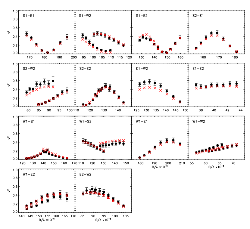
Figure 1: Squared visibilities of $\sigma$ Orionis measured with MIRC at the CHARA Array on UT 2011 September 29 (filled black circles). The red crosses indicate the visibilities derived from the best-fit scaled binary model. The observations have been averaged over 5 min observing blocks. The S1-S2 baseline has been excluded from the fit (see text).

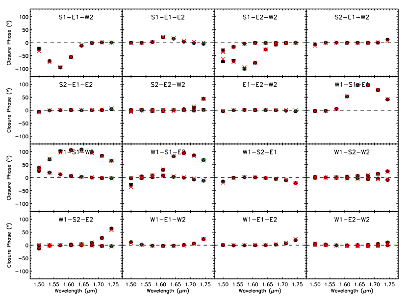
Figure 2: Closure phases of $\sigma$ Orionis measured with MIRC at the CHARA Array on UT 2011 September 29 (filled black circles). The red crosses indicate the closure phases derived from the best-fit scaled binary model. The observations have been averaged over 5 min observing blocks. Closure triangles that include the S1-S2 baseline have been excluded from the fit (see text).

2.2 CHARA Astrometric Results

The diffraction limit of a single 1 m CHARA telescope in the $H$-band corresponds to $\sim$ 0$\farcs$4 on the sky. Therefore, light from all three components in the $\sigma$ Orionis triple (Aa, Ab, B) is recorded in the field of view of the detector (set by the injection of light into the optical fibers of MIRC). However, given the width of the MIRC spectral channels ($\Delta\lambda\sim 0.035$ $\mu$m) and the corresponding coherence length ($\lambda^{2}/\Delta\lambda\sim 75$ $\mu$m), the wide 0$\farcs$25 component $\sigma$ Ori B contributes only incoherent light on all but the shortest baselines, degrading the fringe amplitude by a constant amount set by the percentage of light coming from the wide component. For the shortest baselines (e.g., S1-S2 with a baseline length of 34 m), light from the wide component adds coherently to produce additional periodic variations in the visibilities and closure phases. To simplify the model fitting, we excluded from the fit the S1-S2 baseline and all closure triangles that included both the S1 and S2 telescopes.

A binary star produces a periodic signal in the complex fringe visibilities (Boden, 2000). The presence of the wide third component adds incoherent flux that can be accounted for by scaling the complex visibilities,

$$V=\frac{f_{1}V_{1}+f_{2}V_{2}\exp{[-2\pi i(u\Delta\alpha+v\Delta\delta)]}}{(f_{1}+f_{2}+f_{3})}$$ (1)

where ($\Delta\alpha,\Delta\delta$) are the close pair binary separation in R.A. and Decl., ($u,v$) are the baseline components projected on the sky, $V_{1}$ and $V_{2}$ are the uniform disk visibilities of the primary and secondary components with angular diameters $\theta_{1}$ and $\theta_{2}$, and $f_{1}$, $f_{2}$, and $f_{3}$ are the flux fractions from each of the three components ($f_{1}+f_{2}+f_{3}=1$). When $f_{3}$ is non-zero, the peaks in the periodic visibility curves no longer rise to 1. The real and imaginary parts of the complex visibility are combined to form the squared visibility amplitude between each pair of telescopes and the closure phase for each set of three telescopes. We fit the squared visibility amplitudes and closure phases measured with MIRC using this scaled binary model, assuming angular diameters for the component stars of $\theta_{\rm Aa}=0.27$ mas and $\theta_{\rm Ab}$ = 0.21 mas (see Section 4.2). The adopted values are larger than the angular diameters predicted by Simón-Díaz et al. (2015, 0.14 mas and 0.12 mas). However, because the stellar diameters are unresolved by the interferometer, the effect on the model fitting is small. The flux contributions change by about 1$-$2%, while the binary positions remain consistent within the 1 $\sigma$ uncertainties.

We followed an adaptive grid search procedure (similar to the method described in Gallenne et al., 2015) where we searched through a grid of separations in R.A. and Decl. and performed a Levenberg-Marquardt least-squares minimization using the IDL mpfit routine (Markwardt, 2009) to determine the best fit binary solution for each step in the grid. We retained the solution with the lowest $\chi^{2}$ and examined the $\chi^{2}$ space to check for possible alternative solutions. For most epochs we found a unique solution with a second minimum reflected through the origin but with the fluxes of the components in the close pair flipped (no other solutions were typically found within $\Delta\chi^{2}>100-10,000$ from the best fit). For the data taken on UT 2013 November 3, we found an alternative solution with $\Delta\chi^{2}$ = 12 from the best fit solution; in addition to the higher $\chi^{2}$, the alternative position is not consistent with the orbital motion mapped in Section 4.1. On UT 2010 November 4, we found multiple solutions in the $\chi^{2}$ maps with $\chi^{2}<25$. This was likely caused by a combination of the limited $(u,v)$ coverage during the observation and poor data calibration because of possible alignment drifts during the long time interval to find fringes combined with poor seeing conditions as the target was setting (altitude $\sim$ 36^∘). Because of the ambiguities in the solutions, we do not report a position for this night.

Table 3 lists the separation $\rho$, position angle $\theta$ (measured east of north), and component flux contributions during each of the MIRC observations obtained at the CHARA Array. Uncertainties in the binary positions were computed from the covariance matrix and include correlations between the binary separation in R.A. and Decl. In Table 3, we report the semi-major axis, semi-minor axis, and position angle of the major axis of the error ellipse ($\sigma_{\rm maj},\sigma_{\rm min},\phi$, respectively). We compared these uncertainties against $\chi^{2}$ maps generated from a two-dimensional grid search using fixed steps in separation; the error ellipses are in agreement with the size and orientation of the 1 $\sigma$ ($\Delta\chi^{2}=1$) confidence intervals from the $\chi^{2}$ maps. On average, the components contribute a mean of 47.7% $\pm$ 5.9% (Aa), 27.4% $\pm$ 5.2% (Ab), and 24.9% $\pm$ 8.0% (B) of the total light recorded on the detector in the $H$-band. These fractional flux contributions are very similar to those in the $V$-band as estimated by Simón-Díaz et al. (2015), $48\%$, $28\%$ and $24\%$, respectively.

The larger uncertainties derived for the binary positions on 2013 November 3 and 11 are likely caused by a combination of poor seeing conditions that made finding and tracking the fringes difficult, and the limited $(u,v)$ coverage obtained from the smaller number of telescopes on which fringes could be found. The binary position is expected to change more rapidly on these nights since the companion is near periastron, however, the expected motion on the sky during the time-frame of the observations is smaller than the measurement uncertainties. Breaking the data into smaller time blocks that were fit independently resulted in positions that varied randomly with even bigger error ellipses. Therefore we report the average positions based on the fit to all measurements on each night.

As a check on our results, we also fit the MIRC data using a triple model that includes the relative separation between all three components, $\sigma$ Ori Aa,Ab,B. To minimize the effects of time smearing, we used calibrated data files that were averaged over shorter 2.5 min observing blocks. To account for time smearing across the observing blocks, we computed the triple model at 10 second intervals and averaged over the complex visibilities. We also accounted for bandwidth smearing which reduces the fringe coherence at separations comparable to the width of the fringe packet following the formalism in Kraus et al. (2005). Summing the visibilities at the location of each component, the complex visibility of a triple system is given by,

$$V = \big{[}f_{1}c_{1}(\tau)V_{1}e^{-2\pi i(u\Delta\alpha_{1}+v\Delta\delta_{1})}$$ (2)

$$+f_{2}c_{2}(\tau)V_{2}e^{-2\pi i(u\Delta\alpha_{2}+v\Delta\delta_{2})}$$

$$+f_{3}c_{3}(\tau)V_{3}e^{-2\pi i(u\Delta\alpha_{3}+v\Delta\delta_{3})}\big{]}\times\frac{1}{f_{1}+f_{2}+f_{3}}~{}~{}~{}~{}~{}~{}$$

where $(\Delta\alpha_{n},\Delta\delta_{n})$ are the separations in R.A. and Decl. between the primary, secondary, and tertiary components ($n$ = 1, 2, 3) and the phase center. In the analysis of the MIRC data, we assumed the phase center to be the photocenter of $\sigma$ Ori Aa,Ab. The coherence for a rectangular bandpass profile is given by

$$c_{n}(\tau)=\frac{\sin{(\pi\tau_{n}\Delta\lambda/\lambda^{2})}}{\pi\tau_{n}\Delta\lambda/\lambda^{2}}$$ (3)

where the optical path length delays are given by

$$\tau_{n}=\lambda(u\Delta\alpha_{n}+v\Delta\delta_{n})$$ (4)

and $\Delta\lambda$ is the width of the wavelength channel and $\lambda$ is the central wavelength.

The triple model reproduces the variation in the visibilities and closure phases on the baselines and triangles that include the S1 and S2 telescopes as shown in Figure 3. However, the triple fit is further complicated by changes in seeing and telescope-dependent tip-tilt corrections that influence the measured photocenter of the system and the corresponding phase shift of the fringes. The wide component is over-resolved on the longer baselines, so it is primarily the short S1-S2 baseline that samples the wide pair separation. Because of this limited baseline coverage on the sky, the $\chi^{2}$ maps for the wide component separation sometimes have multiple peaks that are consistent with the data. On the other hand, the close pair separations derived from the triple model are stable and within the uncertainties of those from the scaled binary fit. We opted to report the simpler scaled binary solution as our final results.

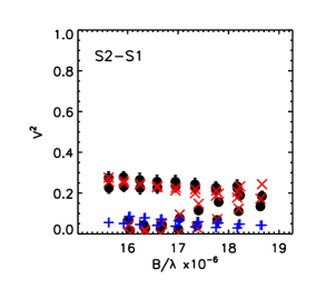
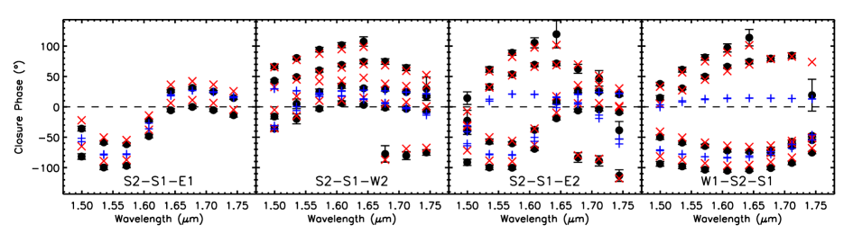
Figure 3: Squared visibilities (left) and closure phases (right) of $\sigma$ Ori measured with MIRC at the CHARA Array on UT 2011 September 29 (black circles). We show only the shortest baseline and closure triangles that include the S1-S2 telescopes. The observations have been averaged over 2.5 min observing blocks. The blue plus signs show the best-fit scaled binary model fit to all baselines and triangles. The observations obtained with the shortest baseline are fit much better by a triple model (red crosses) that directly includes the position of the wide companion $\sigma$ Ori B.

2.3 VLTI Observations and Data Reduction

$\sigma$ Orionis was observed with the AMBER (Petrov et al., 2007) beam combiner at the VLTI (Schöller, 2007) using the Antu (UT1), Kueyen (UT2) and Yepun (UT4) 8.2 m telescopes on UT 2008 October 14 (HJD 2454753.7). The data were recorded with the low-resolution mode ($R=35$) in the $H$ and $K$ bands. The longest baseline between UT1 and UT4 is nominally 130 m in length. A single observation of the science target was sandwiched between two calibrator observations, one of HD 34137 and the other of HD 36059, with diameters of $0.73\pm 0.02$ mas and $0.51\pm 0.01$ mas, respectively (Bonneau et al., 2006, 2011). The data were reduced using the amdlib pipeline (Tatulli et al., 2007; Chelli et al., 2009) but only the top 30% visibility data in terms of signal-to-noise ratio were used to reduce the influence of periods of poor group-delay fringe tracking. Seeing was 0$\farcs$8 on average, but vibrations present in the UT infrastructure limited the fringe contrast. The transfer function was linearly interpolated between the two calibrator measurements to the epoch of the science observation.

With a field of view of about 60 mas with the UTs, AMBER only sees the close pair. The measured separation and position angle are $\rho=4.30\pm 0.52$ mas and $\theta=174\fdg 70\pm 4\fdg 7$. The fit to the data is shown in Fig. 4. The fitted magnitude difference between Ab and Aa is $0.57\pm 0.03$ in the $H$ band and $0.55\pm 0.02$ in the $K$ band. The $H$ band value is consistent with the CHARA value of $\Delta H=0.60$ mag.

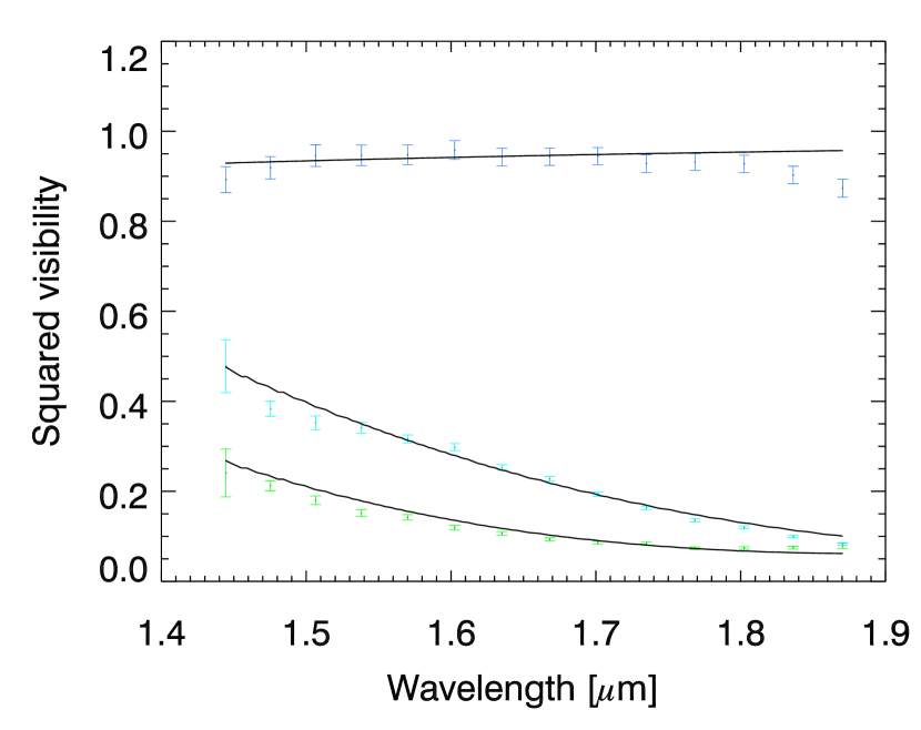
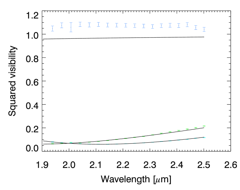
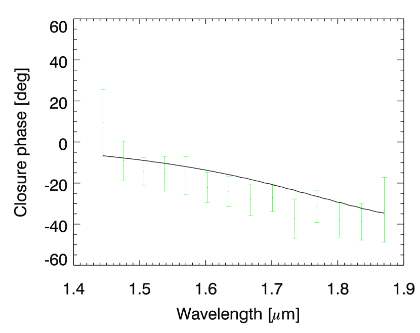
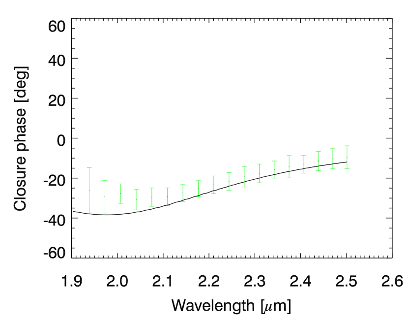
Figure 4: AMBER $H$ and $K$ (squared) visibilities and closure phases. Each color in the visibility plots represents a different baseline pair. The best-fit binary model is overplotted as the solid black line.

2.4 NPOI Observations and Data Reduction

NPOI observations (Armstrong et al., 1998) of $\sigma$ Orionis were collected over a period from 2000 to 2013. Initially, the observations were obtained with the 3-beam combiner, and then, starting in 2002, with the 6-beam hybrid combiner (Benson et al., 2003). The NPOI beam combiners disperse the light and record the visibility spectra from 550 nm to 850 nm in 16 spectral channels. In total, some 59 nights of observations were executed, of which 26 nights were of good quality. Observations of calibrator stars were interleaved with the science target. Table 4 gives information on dates, configurations, and calibrator stars observed for each night. A configuration is given as a triple of stations (e.g. “AC-AE-W7”, using astrometric stations Center and East, as well as imaging station W7) if data from all three baselines were used, including the corresponding closure phase. If a single baseline is listed, squared visibility data from that baseline were used but no closure phase data were available involving this baseline.

The calibrators were selected from a list of single stars maintained at NPOI with diameters estimated from $V$ and $(V-K)$ using the surface brightness relation published by Mozurkewich et al. (2003) and van Belle et al. (2009). Estimates for $E(B-V)$ derived by comparison of the observed colors to theoretical colors as a function of spectral type as given by Schmidt-Kaler in Aller et al. (1982) were used to derive extinction estimates $A_{V}$. These were compared to measurements based on maps by Drimmel et al. (2003) and used to correct $V$ if the two estimates agreed within 0.5 magnitudes. Even though the surface brightness relationship based on $(V-K)$ colors is to first order independent of reddening, we included this small correction because our principal calibrator, $\epsilon$ Orionis (HD 37128), is a B-supergiant at more than 400 pc distance and has a predicted apparent diameter of 1.01 mas. Based on an analysis of calibrator stars observed using the Mark III interferometer, Mozurkewich et al. (1991) measured uniform disk diameters of 0.86 mas $\pm$ 0.16 mas (at 800 nm) and 1.02 $\pm$ 0.12 mas (at 450 nm) for $\epsilon$ Orionis. However, because the star was barely resolved on the Mark III baselines (up to 38 m in length), we decided to use our estimate as the more precise value. On the longest NPOI baseline that we used (E6-W7, 79 m), and in the middle of the bandpass (700 nm), the expected squared visibility of $\epsilon$ Orionis is 0.45. The information for all of the calibrators is given in Table 5.

The NPOI data and their reduction were described by Hummel et al. (1998, 2003). We used an new version of the OYSTER NPOI data reduction package written in GDL. The pipeline automatically edits the 1-second averages produced by another pipeline directly from the raw frames, based on expected performance such as the variance of fringe tracker delay, photon count rates, and narrow angle tracker offsets. Visibility bias corrections are derived as usual from data recorded away from the stellar fringe packet. After averaging the data over the full length of an observation, the closure phases and the transfer function of the calibrators were interpolated to the observation epochs of $\sigma$ Orionis. For the calibration of the visibilities, the pipeline used all calibrator stars observed during a night to obtain smooth averages of the amplitude and phase transfer functions using a Gaussian kernel of 80 minutes in length. The residual scatter of the calibrator visibilities and phases around the average set the level of the calibration uncertainty and was added in quadrature to the intrinsic data errors.

Considerable effort was invested in algorithms that automatically edit the visibility data based on the variance of the delay-line positions following the procedures described by Hummel et al. (2003, Section 4.2) and adapted to more complicated source structures where the signal-to-noise ratio is low. Especially in the case of $\sigma$ Orionis, deep visibility minima exist on the baselines typically employed by our observations. A final step was therfore added to detect problems by comparing the results to the predictions of the final model derived later from all data sets. An amplitude calibration error of typically a few percent in the red channels and up to 15% in the blue channels was added in quadrature to the intrinsic error of the visibilities. The phase calibration was good to $\sim 2^{\circ}$. Nevertheless, because of small changes in atmospheric conditions between the observations of the calibrators and the science target we used additional baseline-based calibration factors (“floating calibration”) to allow minor adjustments of the visibility spectra to obtain better fits to the orbital elements (and magnitude differences) of the triple system. Two thirds of the spectra were adjusted by less than 25%, the remainder were mostly low SNR spectra. Because the components of $\sigma$ Orionis Aa, Ab, and B are unresolved (see Section 4.2), the maximum visibility amplitude was fixed to unity. This procedure will not bias the astrometric results because the binary separation is constrained mostly by the variation of the visibility data with wavelength (Fig. 5). The magnitude differences between the components across the 550$-$850 nm band were determined to be 0.5 $\pm$ 0.1 mag for Ab$-$Aa and 1.5 $\pm$ 0.2 mag for B$-$A. We assumed that the magnitude differences between the components are the same across the $V$ and $I$ bands; this is expected since both components are hot stars and should have similar colors.

2.5 NPOI Astrometric Results

Because of the large angular separation of the tertiary component ($\sigma$ Ori B), rapid variations of the visibility amplitude occur on the shorter NPOI baselines, while they are completely smeared out on the longer baselines due to the finite width of the spectral channels. The number of fringes in the central envelope of an interferogram is given by $N=2\lambda/\Delta\lambda=2R$ where $\Delta\lambda$ is the width of the bandpass and $R$ is the equivalent spectral resolving power of the spectrometer. The fringe amplitude decreases to zero towards the edge of the envelope. One fringe spacing corresponds to $\lambda/B$ radians on the sky, where $B$ is the projected baseline length. Since the smallest baselines employed for our observations are about 20 M$\lambda$ long (in the reddest channel at 850 nm), the fringe spacing is about 10 mas, and thus the field of view is about 300 mas in diameter if we consider a loss in (squared) amplitude of about 60% and $R=30$ for the NPOI spectrometers. Since the NPOI channel bandpasses are known, complex visibilities predicted by a model of the triple system are computed on a sufficiently fine wavelength grid, and then averaged over the bandpasses before converting them to squared visibilities and closure phase for comparison to the observed quantities.

An example of the rapid variations of the (squared) visibility amplitude on the AN0-W7 baseline is shown in Figure 5, together with the predicted values from our final model (discussed in Section 4.2). Small errors in the predicted position of the tertiary relative to the close binary can lead to significant deviations between the data and the model. Therefore, we first improved our knowledge of the tertiary orbit. The elements published by Turner et al. (2008) were based on adaptive optics and speckle measurements, the last of which dates back to the end of 2001. While our NPOI observations started around the same time, the early data sets did not allow for the unambiguous identification of the location of the tertiary (if detected at all) because of the close and regular spacing of the local minima in the $\chi^{2}$ surface which is caused by undersampling of the fast variations of the visibility amplitude in combination with often parallel orientation of the baselines relative to the direction of the tertiary. The first night to provide an unambiguous identification of the position of the tertiary was on 2010 March 25, as one of the baselines, AN0-W7, rotated close to an orthogonal orientation to the wide binary orientation, causing a change in the “wavelength” of the visibility oscillation (seen in Fig. 5). We then added this epoch to the measurements of $\sigma$ Ori A,B available from the Washington Double Star Catalog and refit the orbital elements. Subsequently, five more nights were identified with similar quality, and were used to refine the orbital elements. Finally, all nights with a pronounced minimum of $\chi^{2}$ at the predicted position of the tertiary were included in the fit. The results are given in Table 6 which gives the date, Julian year of the observation (at 7 UT), the number of measured visibilities, the derived separation (relative to the center of mass of the close pair), position angle, and the semi-axes and position angle of the uncertainty ellipses. The last two columns give the deviation of the fitted relative binary position $(\rho,\theta)$ from the model values. The uncertainty ellipses were computed from fits to contours of the $\chi^{2}$ surfaces near the minima rather than deriving them from the interferometric PSF. This accounts for the limitations of fitting a component position very far from the phase center. We scaled the contours to result in a reduced $\chi^{2}$ of unity at the minimum. The positions of $\sigma$ Ori A,B are in good agreement with measurements made at similar times by Simón-Díaz et al. (2015) and Aldoretta et al. (2015).

Figure 5: NPOI squared visibilities for 2010 March 25. Panels a-f correspond to observations at 03:38, 03:42, 04:08, 04:17, 04:32, and 04:36 UT. The data shown are for baseline AN0-W7.

After the orbit of the tertiary was revised, astrometric positions of the secondary were fit to the visibility data for each night separately (with fixed tertiary positions derived from the tertiary orbit). Error ellipses were estimated using the $\chi^{2}$ surface maps centered on the position of the secondary. The $\chi^{2}$ contour interval was selected to give a reduced $\chi^{2}$ close to unity when fitting the astrometric positions with an orbit for the close pair. This resulted in using the $\Delta\chi^{2}=40$ confidence interval. Correlations in the visibility amplitudes between the 16 channels, related to atmospheric seeing variations, reduces the number of independent data points and explains partly the size of this interval. Table 7 lists the results for the separation and position angle of $\sigma$ Ori Aa,Ab derived from the NPOI data, the semi-axes and position angle of the uncertainty ellipses, and the residuals compared with the orbit fit.

3 CTIO Spectroscopy

We obtained new spectrocopic radial velocity measurements of $\sigma$ Orionis Aa,Ab using the 1.5 m telescope at CTIO. We obtained 40 observations on 29 nights using the Fiber Echelle (FE) Spectrograph ($R=25,000$, $\lambda$ = 4800–7000 Å) between UT 2008 September 23 and 2009 February 21. Additional observations were obtained using the Chiron fiber-fed echelle spectrometer (Tokovinin et al., 2013) equipped with an image slicer ($R=78,000$, $\lambda$ = 4550–8800 Å) on 10 nights between UT 2012 November 4 and 2013 February 2 and 11 nights between UT 2016 January 21 and March 27. The Chiron observations were concentrated near periastron passage of the close pair.

All of the spectra were corrected to a heliocentric velocity scale prior to measurement. For the FE data, we measured the velocities of the He I 5876 line because it is in the same order as the interstellar Na I D lines, which provide a good velocity fiducial. For the Chiron data, we fit five He I lines ($\lambda\lambda$ 4713, 4921, 5876, 6678, and 7065 Å) and He II ($\lambda=4686$ Å). The He I lines are stronger in the cooler, less massive component while He II is stronger in the more rapidly rotating hotter star. We fit two Gaussian components to each line to measure the radial velocities of both components. We allowed the central wavelength, width, and amplitude of the Gaussian components to vary independently for each fit. The He II 4686 and He I 6678 line profiles are fairly clean, while contamination from weak lines from the cooler star in the three bluest He I lines required fitting up to three additional Gaussian components. We treat these additional components as nuisance parameters. Telluric lines are present at 5876 Å and are a significant problem at 7065 Å. We generated a telluric spectrum by filtering these spectra with a low-pass filter to remove the higher frequency narrow lines while preserving the He I line profiles, and then fit these “cleaned” spectra.

To check the wavelength stability, we measured the insterstellar Na D1 and D2 lines in all of the spectra. At the lower resolution of the FE, contamination by the telluric lines can distort the Na D profiles as they shift due to the heliocentric correction. In fact, there is a small annual distortion in the measured velocity of the Na D lines in the FE spectra. The median radial velocities measured from the FE spectra are $21.72\pm 0.41$ km s^-1 for Na D1 and $22.63\pm 0.69$ km s^-1 for Na I D2, where the uncertainties are the standard deviations from the mean. With the higher resolution Chiron spectra we were able to fit both interstellar components (a weaker line at about $+10$ km s^-1) and avoid the stronger telluric features. The stronger lines have stable radial velocities with a median of $22.55\pm 0.21$ km s^-1 for Na D1 and $22.54\pm 0.19$ km s^-1 for Na D2. The Chiron instrumental resolution is about 3.8 km s^-1. There seem to be no significant offsets between the two instrument zero-points. Hobbs (1969) resolved the Na D lines into two components with velocities of 20.5 and 24.0 km s^-1 at higher spectral resolution ($\sim$ 0.51 km s^-1 ); these would average to 22.3 km s^-1, consistent with our measurements.

The median radial velocities of $\sigma$ Ori Aa and Ab, measured from the selected spectral lines, are presented in Table 8. Based on the Gaussian line widths, we derived rotational velocities of $v\sin{i}\approx 125$ km s^-1 for Aa and $v\sin{i}\approx 43$ km s^-1 for Ab (assuming no limb-darkening). We did not fit for the weak and broad stationary lines from $\sigma$ Ori B, which are difficult to detect without detailed modeling (Simón-Díaz et al., 2011, 2015). Because the spectral profiles of $\sigma$ Ori B are so shallow, their presence creates only a slight depression of the continuum near line center and has little influence on the velocity measurements of components Aa and Ab.

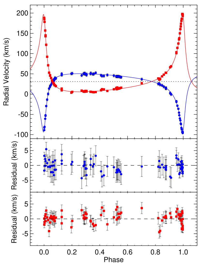
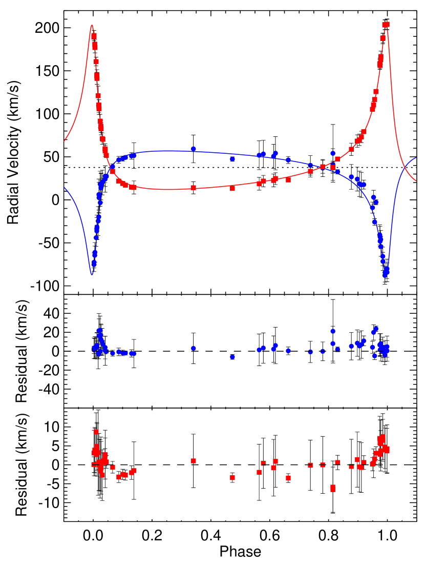
Figure 6: Radial velocities of $\sigma$ Orionis Aa,Ab published by Simón-Díaz et al. (2015, left) and measured at CTIO (right). The blue circles show the velocities measured for Aa and the red squares show the velocities for Ab. Overplotted are the radial velocity curves derived from the simultaneous orbit fit to both sets of spectroscopic data and the interferometric positions measured at the CHARA Array. The residuals for each component are shown in the lower panels.

The first two columns of Table 9 show the spectroscopic orbital parameters derived by Simón-Díaz et al. (2015) compared with those derived from the CTIO radial velocities. There are systematic differences between the radial velocity semi-amplitudes ($K_{Aa}$, $K_{Ab}$) and the systemic velocity $\gamma$ derived from each set of data. Simón-Díaz et al. cross-correlated the spectra against atmospheric models, fitting many lines simultaneously, which could account for the higher precision of their velocity semi-amplitudes. The systematic differences could result from the different methods used to fit the blended lines, as well as differences in the wavelength calibration. A comparison of the radial velocity measurements is shown in Figure 6. A simultaneous orbit fit to both sets of data, along with the interferometric positions, is discussed in Section 4.1.

4 Orbits and Derived Properties of the $\sigma$ Orionis Triple

4.1 Visual and Spectroscopic Orbit of the Close Pair $\sigma$ Orionis Aa,Ab

We fit a simultaneous orbit to the higher precision interferometric positions of $\sigma$ Orionis Aa,Ab measured with CHARA in Table 3, the published radial velocities reported by Simón-Díaz et al. (2015), and the CTIO radial velocities in Table 8. We compare the fit to the NPOI positions of the close pair in Section 4.2. Before computing the joint orbit fit, we fit each set of data independently and scaled the measurement uncertainties to force the reduced $\chi^{2}_{\nu}=1$ for each of the CHARA and two radial velocity sets. The measurement uncertainties in the interferometric positions were increased by a factor of 2.24, indicating that the error bars from the covariance matrix are underestimated; we report the scaled uncertainties in Table 3. The reduced $\chi^{2}_{\nu}$ for the radial velocity data from Simón-Díaz et al. (2015) was already close to 1, so we did not adjust those uncertainties. The measurement errors for the CTIO radial velocities were decreased by a factor of 0.66 (the uncertainties listed in Table 8 are the unscaled values). Using the scaled uncertainties, we then fit the measured positions and radial velocities simultaneously using a Newton-Raphson method to minimize $\chi^{2}$ by calculating a first-order Taylor expansion for the equations of orbital motion. The last column of Table 9 provides the orbital parameters determined from the joint fit, including the period $P$, time of periastron passage $T$, eccentricity $e$, angular semi-major axis $a$, inclination $i$, position angle of the line of nodes $\Omega$, argument of periastron passage for the primary $\omega_{\rm Aa}$, and the radial velocity amplitudes of the primary and secondary $K_{Aa}$ and $K_{Ab}$. We allowed for a shift in the systemic velocity $\gamma$ between the two sets of spectroscopic radial velocities. Figures 6 and 7 show the simultaneous spectroscopic and visual orbit fits. The orbital phase and radial velocity residuals for the simultaneous fit are listed in Table 8. For comparison, we also list in Table 9 the orbital parameters determined from the fits to each set of data independently. The velocity amplitudes derived from the joint fit depend more on the higher precision radial velocities published by Simón-Díaz et al. (2015) than on the CTIO radial velocities.

The uncertainty in the wavelength calibration of $\pm$0.25% for MIRC (Monnier et al., 2012), will systematically increase or decrease the angular separations measured for the close pair. To account for this, we varied all of the separations systematically by $\pm$0.25% and re-fit the orbital parameters. The second uncertainty listed for the semi-major axis for the simultaneous fit in Table 9 shows the size of the systematic uncertainty on the orbital fit.

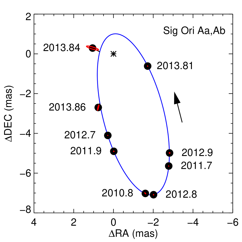
Figure 7: Visual orbit of $\sigma$ Orionis Aa,Ab based on the simultaneous fit to the interferometric positions measured using the MIRC beam combiner at the CHARA Array, the radial velocities published by Simón-Díaz et al. (2015), and the CTIO radial velocities. The black circles mark the position of the companion Ab relative to Aa while the red ellipses show the size and orientation of the 1 $\sigma$ uncertainties. The arrow indicates the direction of motion.

4.2 Visual Orbit of the Wide Pair $\sigma$ Orionis A,B

As discussed in Section 2.5, we computed the orbital elements for the tertiary orbit ($\sigma$ Ori A,B) based on the positions derived from the NPOI data (Table 6) together with all available measurements from the Washington Double Star Catalog. The orbital elements are given in Table 10. The tertiary orbit is shown with the NPOI measurements in Figure 8 and all available measurements in Figure 9. We used the Levenberg-Marquardt method for fitting the orbital elements to the data.

In addition to measuring the positions of the secondary and tertiary components during each individual night, we also fit the orbital parameters directly to the NPOI visibility data. This has the advantage of better constraining the system parameters which do not change from night to night. We used the Levenberg-Marquardt procedure (Press et al., 1992) to perform a non-linear least-squares fit to the visibility data and solved simultaneously for the orbital parameters for both orbits (Aa,Ab and A,B) and the magnitude difference between each component. We fixed the component diameters at values of 0.27 mas, 0.21 mas, and 0.17 mas for components Aa, Ab, and B, respectively. These diameters were estimated based on their $V$ magnitudes (derived from the fitted magnitude differences and the total magnitude of the system $V=3.80$ mag) and adopting the same $(V-K)$ color of $-0.69$ for all three components (as they are all of early type; derived using the total magnitude of the system of $K=4.49$ mag). Such small diameters are unresolved on the baselines used during our observations. Because of the large number of fit parameters, the numerical partial derivatives of $\chi^{2}$ with respect to the model parameters were based on step sizes optimized to give similar increases in $\chi^{2}$ for each parameter. The reduced $\chi^{2}$ of the fits to the visibility data was 1.66 ($\chi^{2}=3.1$ without the floating calibration). The orbital elements of $\sigma$ Orionis Aa,Ab derived from the NPOI data agree with the parameters derived from the CHARA data within 0.1$-$2.0 $\sigma$, but are less precise so we do not report the NPOI parameters explicitly. However, Figure 10 shows that the NPOI astrometric positions are in good agreement with the CHARA orbit.

When the tertiary is detected by the NPOI, it can be used as a phase reference to measure the absolute motions of component Aa and Ab relative to their center of mass. This provides an independent estimate of their mass ratio $M_{\rm Ab}/M_{\rm Aa}$. In Fig. 11 we show the reduced $\chi^{2}$ of the fit to the NPOI visibility data as a function of the mass of Ab, which shows a minimum at $M_{\rm Ab}=13.5\pm 0.4$ $M_{\odot}$, assuming a fixed mass for the primary of the $M_{\rm Aa}$ = 16.9 $M_{\odot}$. Away from this value, the relative positions of the three components change as the center of mass of the close binary shifts because of the change in the mass ratio between Aa and Ab. As a check, we also show that the $\chi^{2}$ does not vary with tertiary mass, as may be expected from the fact that this changes only the phase center of the triple system. Given the uncertainty of $M_{\rm Ab}$ fit to the NPOI data, we do not consider the difference from the value of the dynamical mass derived in Section 4.3 to be significant.

Figure 8: Orbital motion of the tertiary component ($\sigma$ Ori B) relative to the photo-center of the close pair ($\sigma$ Ori Aa,Ab). The error ellipses show the positions measured with NPOI in Table 6. The solid line is the best-fit orbit and the dashed line is the orbit computed by Turner et al. (2008).

Figure 9: Orbit of the tertiary ($\sigma$ Ori B) shown with all of the measurements available in the Washington Double Star Catalog. The high precision measurements in the north-east (upper-left) quadrant are the AstraLux measurements published by Simón-Díaz et al. (2015). The solid line indicates periastron and the arrow shows the direction of motion.

Figure 10: Orbital positions of $\sigma$ Ori Ab relative to Aa as measured from the NPOI observations. The single VLTI AMBER observation is included as well ($\Delta\alpha=0.5$ mas, $\Delta\delta=-4.5$ mas). Overplotted is the orbit determined from the analysis of the CHARA MIRC observations.

Figure 11: Reduced $\chi^{2}$ as a function of secondary mass (top panel; $\sigma$ Ori Ab) and tertiary mass (bottom panel; $\sigma$ Ori B).

4.3 Stellar Masses and Distance

Using the orbital parameters of the close pair $\sigma$ Ori Aa,Ab in Table 9, we derive dynamical masses of $M_{\rm Aa}$ = 16.99 $\pm$ 0.20 $M_{\odot}$ and $M_{\rm Ab}$ = 12.81 $\pm$ 0.18 $M_{\odot}$. The orbital parallax of $\pi$ = 2.5806 $\pm$ 0.0088 mas gives a distance $d=$ 387.5 $\pm$ 1.3 pc to the $\sigma$ Orionis system. The total mass contained in the triple can be derived from the orbital parameters of the wide pair $\sigma$ Ori A,B in Table 10 and the orbital parallax $\pi$,

$$M_{\rm tot} = M_{\rm Aa}+M_{\rm Ab}+M_{\rm B}=a_{\rm AB}^{3}/(\pi^{3}P^{2}_{\rm AB})$$

$$= 41.4\pm 1.1~{}M_{\odot}.$$

Combined with the individual masses of Aa and Ab, this yields the mass of the tertiary component of $M_{\rm B}$ = 11.5 $\pm$ 1.2 $M_{\odot}$. The derived physical properties of the $\sigma$ Orionis system are summarized in Table 11.

5 Discussion

5.1 Comparison of stellar masses with evolutionary models

Simón-Díaz et al. (2015) compared spectroscopically derived physical properties of $\sigma$ Ori Aa, Ab, and B with evolutionary tracks for rotating stars in the Milky Way computed by Brott et al. (2011) to derive evolutionary masses of $M_{\rm Aa}$ = 20.0 $\pm$ 1.0 $M_{\odot}$, $M_{\rm Ab}$ = 14.6 $\pm$ 0.8 $M_{\odot}$, and $M_{\rm B}$ = 13.6 $\pm$ 1.1 $M_{\odot}$. These masses are systematically larger than the dynamical masses we computed in Table 11. Additionally, the ages derived by Simón-Díaz et al. (2015, Aa: 0.3${}^{+1.0}_{-0.3}$ Myr, Ab: 0.9${}^{+1.5}_{-0.9}$ Myr, B: 1.5${}^{+1.6}_{-1.9}$ Myr) are smaller than the typical age adopted for the $\sigma$ Orionis cluster of 2$-$3 Myr (e.g., Sherry et al., 2008). Future progress on resolving the discrepancies in the masses and ages could involve refining the component temperatures and luminosities, or adjusting the input parameters for the evolutionary models, especially because the evolution of massive stars is strongly dependent on their rotation and metallicity (Brott et al., 2011; Ekström et al., 2012).

Weidner et al. (2010) studied the empirical correlation between the mass of a cluster and its most massive member. Our dynamical mass for $\sigma$ Ori Aa of 16.99 $\pm$ 0.20 $M_{\odot}$ provides an additional high precision mass measurement of the most massive member of the $\sigma$ Orionis cluster. Estimates of the total mass of the cluster range from 225 $\pm$ 30 $M_{\odot}$ (Sherry et al., 2004) down to $\sim$ 150 $M_{\odot}$ (Caballero, 2007); these estimates are strongly dependent on the membership selection, assumed reddening, multiplicity, and evolutionary models used to estimate the masses.

5.2 Distance to the $\sigma$ Orionis Cluster

The distance to the $\sigma$ Orionis cluster has remained a large source of uncertainty in determining the age of the cluster and characterizing the physical properties and disk life-times for the stars, brown dwarfs, and planetary-mass members in the region. The Hipparcos parallax of $\sigma$ Orionis itself (2.84 $\pm$ 0.91 mas) yields a distance with a large uncertainty of $352^{+166}_{-85}$ pc (Perryman et al., 1997). The new reduction of the Hipparcos data gives a parallax of 3.04 $\pm$ 8.92 mas (van Leeuwen, 2007a, b), resulting in a slightly smaller distance of 329 pc, but with a much larger uncertainty. $\sigma$ Orionis presents a difficult problem for the Hipparcos analysis as it is bright and occasionally saturated, and the signals from the three components are mixed. This required an individual component solution in the original reduction (ESA, 1997). Such individual attention was not possible in all cases for the new reduction and accounts for the large uncertainty (F. van Leeuwen, 2016, priv. comm.). Nevertheless, the original and new Hipparcos reductions yield parallaxes that agree within the uncertainty of the original reduction. The orbital parallax that we measure is two orders of magnitude more precise and provides an independent check of the Hipparcos parallax for this triple star system and could be of use as a check of GAIA parallaxes for multiple stars.

Several other methods have been used to estimate the distance to $\sigma$ Orionis. Francis & Anderson (2012) computed a distance to the $\sigma$ Orionis cluster of $446\pm 30$ pc based on the average Hipparcos parallaxes measured for 15 members. By comparing the apparent magnitudes and the dynamical mass from the visual orbit of $\sigma$ Ori A,B with evolutionary models, Caballero (2008a) derived a smaller distance of $334^{+25}_{-22}$ pc, or 385 pc if the system is treated as a triple. Using main-sequence fitting to the bright members in the $\sigma$ Orionis cluster, Sherry et al. (2008) derived a distance of $420\pm 30$ pc while Mayne & Naylor (2008) derived a distance of $389^{+34}_{-24}$ pc. The variation in these distance estimates is large, although, for the most part, the values overlap within the range of their 1 $\sigma$ uncertainties. Our distance from the orbital parallax of the $\sigma$ Orionis multiple system of 387.5 $\pm$ 1.3 pc provides a significant improvement in the precision compared with the previous estimates of the cluster distance, and will reduce the uncertainties in future estimates of the age of the cluster based on isochrone fits.

5.3 Alignment of the Inner and Outer Orbits

The alignment of the orbits between the inner and outer pairs in heirarchical multiple systems can probe the initial conditions of star formation (Fekel, 1981; Sterzik & Tokovinin, 2002). The relative inclination between the inner and outer orbits is given by

$$\cos{\Phi} = \cos{i_{\rm wide}}\cos{i_{\rm close}}\pm\sin{i_{\rm wide}}\sin{i_{\rm close}}$$ (5)

$$\times\cos{(\Omega_{\rm wide}-\Omega_{\rm close})}$$

(Fekel, 1981) where $i_{\rm close}$ and $\Omega_{\rm close}$ are the inclination and position angle of the ascending node for the close orbit while $i_{\rm wide}$ and $\Omega_{\rm wide}$ are the same parameters for the wide orbit. Coplanar orbits will have a relative alignment close to $\Phi=0$. For the wide visual pair, $\sigma$ Ori A,B, there exists a 180^∘ ambiguity between $\Omega$ and $\omega$. For the close pair, $\sigma$ Ori Aa,Ab, $\omega$ is defined by the spectroscopic orbit, so there is no ambiguity with $\Omega_{\rm close}$. Using the orbital parameters in Tables 9 and 10, and accounting for the ambiguity in $\Omega_{\rm wide}$, this leads to two possibilities for the relative inclination between the inner and outer orbits of $120\fdg 0\pm 2\fdg 6$ or $126\fdg 6\pm 2\fdg 0$. Therefore, the alignment of the two orbits in the $\sigma$ Orionis triple are within $\sim 30^{\circ}$ of orthogonal. The orbital motion of the inner pair is prograde (in the direction of increasing position angles; Heintz, 1978) while the motion of the outer pair is retrograde, as indicated by the directional arrows in Figures 7 and 9. This situation is not necessarily rare; the inner and outer orbits in the Algol triple are also nearly orthogonal, with opposing directions of motion (Zavala et al., 2010; Baron et al., 2012).

6 Conclusions

We obtained interferometric observations of the triple star $\sigma$ Orionis using the CHARA Array, NPOI, and VLTI. We revised the orbital parameters for the wide A,B pair and present the first visual orbit for the close Aa,Ab pair, fit simultaneously with new and previously published radial velocities. The orbit of the close pair is eccentric ($e\sim 0.78$) but the stars are reliably separated at periastron ($\rho_{\rm min}\sim 0.91$ mas). Through our analysis of the orbital motion in the triple system, we derived dynamical masses of $M_{\rm Aa}$ = 16.99 $\pm$ 0.20 $M_{\odot}$, $M_{\rm Ab}$ = 12.81 $\pm$ 0.18 $M_{\odot}$, and $M_{\rm B}$ = 11.5 $\pm$ 1.2 $M_{\odot}$, and a distance of 387.5 $\pm$ 1.3 pc. The orbital parallax places the $\sigma$ Orionis system about $7\%$ closer to the Sun than the Orion Nebula Cluster, which lies at a distance of $415\pm 5$ pc based on VLBI parallaxes (Reid et al., 2014).

Two other bright members of the Orion OB1b association are also known triples, $\zeta$ Ori (Hummel et al., 2013) and $\delta$ Ori (Richardson et al., 2015). The outer tertiary star appears to be a rapid rotator in each of $\sigma$ Ori ($V\sin i=250$ km s^-1; Simón-Díaz et al., 2015), $\zeta$ Ori ($V\sin i=350$ km s^-1; Hummel et al., 2013), and $\delta$ Ori ($V\sin i=252$ km s^-1; Richardson et al., 2015). This suggests that the angular momentum of the natal cloud was transformed mainly into orbital angular momentum for the stars of the inner binary and into spin angular momentum for the outer tertiary star. It is also possible that these triples began life as trapezium systems of four stars in which dynamical processes led to a merger of one pair that we see today as the distant rapid rotator. Joint interferometric and spectroscopic studies offer the means to determine the outcome products of the dynamical processes of massive star formation.

Table 1: CHARA MIRC Observation Log for $\sigma$ Orionis.

UT Date	HJD $-$	Configuration	Calibrators	Number of	Number of	Seeing
	2,400,000			$V^{2}$	Closure Phases	$r_{0}$ (cm)
2010 Nov 04	55505.061	S2-W1-W2	HD 33256	24	8	6.6
2010 Nov 05	55506.014	S1-W1-W2	HD 33256	48	16	7.3
2011 Sep 29	55834.004	S1-S2-E1-E2-W1-W2	HD 25490, HD 33256	200	240	12.0
2011 Dec 09	55904.836	S1-S2-E1-E2-W1-W2	HD 25490, HD 33256	319	364	6.8
2012 Sep 15	56186.016	S1-S2-E1-E2-W1-W2	HD 33256, HD 43318	240	320	13.2
2012 Oct 31	56231.907	S1-S2-E1-E2-W1-W2	HD 33256, HD 43318	220	248	15.0
2012 Dec 09	56270.813	S1-S2-E1-E2-W1-W2	HD 25490, HD 33256, HD 43318	168	168	6.1
2013 Oct 21	56586.948	S1-E1-E2-W1-W2	HD 25490, HD 33256, HD 43318	205	144	12.1
2013 Nov 03	56599.926	S1-W1-W2	HD 33256, HD 55185	47	11	7.6
2013 Nov 11	56607.886	E1-E2-W1-W2	HD 33256, HD 43318	46	24	10.7

Table 2: Adopted Calibrator Angular Diameters for CHARA MIRC Observations

Calibrator	Angular Diameter	Reference
	(mas)
HD 25490	0.599 $\pm$ 0.020	SED fit - this work
HD 33256	0.655 $\pm$ 0.018	SED fit - this work
HD 43318	0.491 $\pm$ 0.030	Baines et al. (2008)
HD 55185	0.474 $\pm$ 0.014	Mourard et al. (2011)

Table 3: Positions of $\sigma$ Orionis Aa,Ab measured with CHARA MIRC

UT Date	HJD $-$	$\rho$	$\theta$	$\sigma_{\rm maj}$	$\sigma_{\rm min}$	$\phi$	$f_{Aa}$	$f_{Ab}$	$f_{B}$
	2,400,000	(mas)	(deg)	(mas)	(mas)	(deg)
2010 Nov 05	55506.014	7.2007	192.867	0.0430	0.0036	41.16	0.4655 $\pm$ 0.0051	0.2704 $\pm$ 0.0036	0.2640 $\pm$ 0.0062
2011 Sep 29	55834.004	6.2883	206.224	0.0046	0.0031	156.37	0.4347 $\pm$ 0.0029	0.2549 $\pm$ 0.0020	0.3105 $\pm$ 0.0035
2011 Dec 09	55904.836	4.9017	180.184	0.0098	0.0076	132.28	0.4167 $\pm$ 0.0039	0.2477 $\pm$ 0.0037	0.3356 $\pm$ 0.0053
2012 Sep 15	56186.016	4.1128	176.028	0.0047	0.0019	142.73	0.4986 $\pm$ 0.0045	0.2989 $\pm$ 0.0027	0.2025 $\pm$ 0.0053
2012 Oct 31	56231.907	7.3658	195.874	0.0086	0.0032	164.21	0.4145 $\pm$ 0.0033	0.2450 $\pm$ 0.0025	0.3405 $\pm$ 0.0042
2012 Dec 09	56270.813	5.7271	209.509	0.0167	0.0142	175.66	0.4947 $\pm$ 0.0058	0.2976 $\pm$ 0.0067	0.2077 $\pm$ 0.0088
2013 Oct 21	56586.948	1.8253	250.315	0.0072	0.0050	134.36	0.4497 $\pm$ 0.0024	0.2666 $\pm$ 0.0020	0.2838 $\pm$ 0.0031
2013 Nov 03	56599.926	1.0917	74.529	0.3161	0.0524	73.41	0.5992 $\pm$ 0.0497	0.1989 $\pm$ 0.0444	0.2019 $\pm$ 0.0666
2013 Nov 11	56607.886	2.8034	164.128	0.1406	0.0148	166.21	0.5181 $\pm$ 0.0302	0.3888 $\pm$ 0.0300	0.0931 $\pm$ 0.0426

Note. — The size of the major and minor axes of the error ellipse for the binary positions have been scaled by a factor of 2.24

to force $\chi^{2}_{\nu}=1$ for an orbit fit to only the MIRC derived positions. The second column repesents the median HJD for the

time of observation.

Table 4: NPOI Observation Log for $\sigma$ Orionis

			Min. length	Max. length
UT Date	Julian Year	Triangles and baselines	(m)	(m)	Calibrators (HD)
(1)	(2)	(3)	(4)	(5)	(6)
2001 Feb 21	2001.1408	AC-AE-AW	18	36	37128
2001 Feb 22	2001.1435	AC-AE-AW	18	37	37128 56537
2002 Feb 15	2002.1237	AE-AW AW-AC W7-AC	6	49	37128
2006 Nov 08	2006.8529	AC-AE-W7	12	39	25940
2006 Nov 18	2006.8802	AC-AE-W7	10	56	22192 5448 24760 25940
2007 Feb 18	2007.1314	AE-W7 AN0-W7 AW-W7	14	40	37128 87737 91316
2007 Oct 19	2007.7975	AC-AE-AN0	18	49	37128
2007 Oct 20	2007.8000	AE-AC AE-AN0	18	48	17573 37128
2007 Nov 01	2007.8329	AC-AE AC-AW	15	43	17573 37128
2007 Nov 03	2007.8384	AC-AE	17	35	17573 37128
2008 Nov 16	2008.8761	AC-AE-W7	15	52	19994 37128 21790
2008 Nov 17	2008.8788	AC-AE-W7	17	50	19994 37128 21790
2010 Mar 18	2010.2085	AE-AN0-AW AE-AN0-W7	23	53	37128
2010 Mar 21	2010.2167	AE-AN0-AW AE-AN0-W7	22	50	37128
2010 Mar 25	2010.2277	AE-AN0-AW AE-AN0-W7	20	46	37128
2010 Mar 29	2010.2386	AE-AN0-W7 AW-AE	26	47	37128
2011 Jan 29	2011.0766	AC-AW-E6	17	52	24760 37128
2011 Jan 30	2011.0793	AC-AW-E6	17	53	24760 37128
2011 Feb 05	2011.0957	AC-AE AC-E6	19	68	22192 37128 56537 58715
2011 Feb 07	2011.1012	AC-AE AC-E6 AE-W7 E6-W7	18	76	22192 37128 56537 58715
2011 Feb 10	2011.1094	AC-AE-W7 AC-E6-W7	19	73	22192 37128 56537 58715
2011 Feb 11	2011.1121	AC-AE AC-E6 AE-W7	18	66	22192 37128 56537 58715
2011 Feb 12	2011.1148	AC-AE-W7 AC-E6-W7	18	79	22192 37128 56537 58715
2011 Feb 13	2011.1175	AC-E6 E6-W7	19	79	22192 37128 56537 58715
2011 Mar 13	2011.1941	E6-AC	17	47	37128 56537 58715
2011 Mar 16	2011.2022	AW-AC E6-AC	18	49	37128 56537 58715
2011 Dec 10	2011.9393	AE-AW-E6 W7-AW	16	74	23408 23862 37128 56537
2012 Jan 04	2012.0075	AE-AW E6-AW W7-AW	15	70	23408 23862 37128 56537
2013 Jan 17	2013.0451	AC-AW-E6	17	53	58142 24760 37128 50019
2013 Feb 01	2013.0861	AC-AW-E6	17	53	22192 24760 37128

Note. — The second column is median Julian Year at the time of the observations.

Table 5: NPOI Calibrators.

HD	Spectral	$V$	$V-K$	$E(B-V)$	$\theta_{V-K}$	$V^{2}_{\rm min}$	Nights
	Classification	(mag)	(mag)	(mag)	(mas)
HD 886	B2IV	2.83	-0.94	0.01	0.50	0.97	2
HD 5448	A5V	3.87	0.23	0	0.70	0.82	1
HD 11171	F3III	4.65	0.78	0	0.65	0.89	1
HD 17573	B8Vn	3.63	-0.23	0.01	0.55	0.96	3
HD 19994	F8V	5.06	1.31	0.05	0.75	0.84	1
HD 21790	B9Vs	4.74	-0.15	0	0.34	0.96	1
HD 22192	B5Ve	4.23	0.12	0.11	0.51	0.90	5
HD 23408	B8III	3.87	-0.12	0.04	0.50	0.92	2
HD 23862	B7p	5.09	0.15	0.05	0.35	0.96	2
HD 24760	B0.5V	2.88	-0.83	0.11	0.52	0.90	5
HD 25940	B3Ve	4.04	0.24	0.17	0.61	0.86	1
HD 37128	B0Ia	1.70	-0.57	0.04	1.01	0.45	16
HD 50019	A3III	3.60	0.44	0.02	0.80	0.96	1
HD 56537	A3V	3.57	0.03	0.02	0.67	0.72	5
HD 58142	A1V	4.64	0.07	0	0.41	0.99	1
HD 58715	B8Vvar	2.90	-0.20	0.02	0.78	0.63	3
HD 67006	A2V	4.84	0.18	0	0.41	0.95	1
HD 87504	B9III-IV	4.60	-0.13	0	0.37	0.99	1
HD 87737	A0Ib	3.49	0.19	0	0.75	0.76	1
HD 87887	A0III	4.49	0.04	0	0.44	0.99	1
HD 91316	B1Ib	3.85	-0.43	0.05	0.42	0.92	1
HD 97633	A2V	3.34	0.26	0	0.86	0.78	4
HD 98058	A7IVn	4.50	0.37	0	0.54	0.98	1
HD 98664	B9.5Vs	4.06	-0.08	0	0.49	0.99	1
HD 112413	A0pSiEuHg	2.90	-0.24	0	0.76	0.92	4
HD 126129	A0V	5.12	0.05	0	0.33	0.99	1
HD 129174	B9p	4.91	-0.14	0	0.32	0.99	1
HD 130109	A0V	3.72	0.07	0.01	0.64	0.74	3
HD 193432	B9.5V	4.76	-0.05	0	0.37	0.98	1
HD 214923	B8.5V	3.40	-0.17	0	0.63	0.95	2
HD 219688	B5Vn	4.40	-0.36	0.01	0.35	0.95	1
HD 222173	B8V	4.30	-0.15	0	0.42	0.95	1
HD 222603	A7V	4.50	0.44	0	0.56	0.99	1

Note. — The angular diameter $\theta_{V-K}$ was corrected for extinction. $V^{2}_{\rm min}$ is the minimum estimated calibrator visibility based on $\theta_{V-K}$.

Table 6: NPOI Positions for $\sigma$ Orionis A,B.

		Number of	$\rho$	$\theta$	$\sigma_{\rm maj}$	$\sigma_{\rm min}$	$\phi$	O–Cρ	O–Cθ
UT Date	Julian Year	visibilities	(mas)	(deg)	(mas)	(mas)	(deg)	(mas)	(deg)
(1)	(2)	(3)	(4)	(5)	(6)	(7)	(8)	(9)	(10)
2001 Feb 21	2001.1412	276	255.61	109.42	3.10	0.97	165.4	-0.74	-0.5
2001 Feb 22	2001.1440	184	256.43	109.80	2.02	0.63	164.1	0.08	-0.1
2002 Feb 15	2002.1241	45	256.36	107.01	6.72	1.24	168.4	-0.18	-0.5
2006 Nov 08	2006.8524	121	256.55	96.40	0.86	0.65	112.4	0.17	-0.1
2006 Nov 18	2006.8798	234	256.13	96.13	2.06	0.72	166.7	-0.20	-0.3
2007 Feb 18	2007.1316	94	255.20	95.52	0.59	0.42	165.1	-0.95	-0.2
2007 Oct 19	2007.7969	75	256.73	94.08	1.47	0.66	69.2	0.61	-0.2
2007 Oct 20	2007.7997	45	255.83	94.09	1.31	0.66	64.6	-0.29	-0.2
2007 Nov 01	2007.8325	92	255.76	94.12	2.08	0.73	11.1	-0.34	-0.0
2007 Nov 03	2007.8380	136	255.85	94.06	1.79	0.65	7.4	-0.25	-0.1
2008 Nov 17	2008.8784	373	257.09	91.15	4.96	2.25	18.9	0.87	-0.6
2010 Mar 18	2010.2090	1320	254.39	88.44	4.26	0.85	96.8	-1.69	-0.1
2010 Mar 21	2010.2172	1143	257.09	88.48	2.52	0.48	92.8	1.01	-0.1
2010 Mar 25	2010.2282	1455	255.08	88.37	2.11	0.40	117.6	-1.01	-0.1
2010 Mar 29	2010.2391	495	256.70	88.36	2.50	0.40	90.0	0.59	-0.1
2011 Jan 29	2011.0769	668	256.90	86.52	2.67	0.83	11.1	0.59	0.1
2011 Jan 30	2011.0796	633	256.98	86.58	2.48	0.81	9.2	0.64	0.2
2011 Feb 05	2011.0961	58	259.63	85.26	6.66	0.90	16.7	3.16	-1.1
2011 Feb 10	2011.1097	391	256.57	87.06	3.88	1.25	11.5	0.10	0.7
2011 Feb 11	2011.1125	207	256.18	87.43	3.38	0.76	15.0	-0.28	1.0
2011 Feb 12	2011.1152	1479	257.02	86.81	7.59	1.28	17.7	0.56	0.4
2011 Feb 13	2011.1180	348	256.79	86.91	2.00	0.58	170.3	0.34	0.5
2011 Mar 13	2011.1946	30	260.14	84.73	5.44	0.89	16.0	3.87	-1.6
2011 Mar 16	2011.2028	58	257.54	86.38	2.65	0.64	14.1	1.29	0.1
2011 Dec 10	2011.9393	772	256.83	84.17	7.29	1.31	175.3	0.47	-0.4

Note. — The second column is Julian Year at 7 UT on the date of observation.

Table 7: NPOI Positions for $\sigma$ Orionis Aa,Ab

	HJD $-$	Number of	$\rho$	$\theta$	$\sigma_{\rm maj}$	$\sigma_{\rm min}$	$\phi$	O–Cρ	O–Cθ
UT Date	$2,400,000$	visibilities	(mas)	(deg)	(mas)	(mas)	(deg)	(mas)	(deg)
(1)	(2)	(3)	(4)	(5)	(6)	(7)	(8)	(9)	(10)
2006 Nov 18	54057.79	234	6.72	186.56	0.38	0.12	152.6	0.33	-0.7
2007 Feb 18	54149.79	94	2.12	229.95	0.42	0.13	127.7	-0.16	-9.8
2007 Oct 19	54392.79	75	6.93	203.80	0.90	0.18	49.4	0.10	1.1
2007 Nov 01	54405.79	92	5.91	208.04	0.53	0.22	179.4	-0.08	0.3
2007 Nov 03	54407.79	136	5.42	209.85	0.69	0.26	9.5	-0.41	1.2
2008 Nov 16	54786.79	901	7.38	191.22	0.31	0.13	153.2	0.28	-0.6
2010 Mar 18	55273.79	1320	5.18	212.36	0.08	0.06	135.0	-0.01	0.1
2010 Mar 25	55280.79	1455	4.35	217.89	0.09	0.08	135.0	-0.05	0.7
2011 Jan 29	55590.79	668	1.01	309.77	0.30	0.08	0.1	-0.05	2.8
2011 Jan 30	55591.79	633	1.03	326.23	0.47	0.09	6.3	-0.00	4.5
2011 Feb 07	55599.79	270	1.10	123.74	0.53	0.16	2.4	0.03	-7.7
2011 Feb 11	55603.79	207	3.05	169.08	0.76	0.18	11.7	0.92	9.8
2011 Feb 12	55604.79	1479	2.58	163.92	0.20	0.09	2.1	0.20	1.5
2011 Dec 10	55905.79	772	4.73	181.47	0.34	0.10	167.7	-0.28	0.9
2012 Jan 04	55930.79	86	7.15	190.50	0.45	0.14	170.5	0.11	-0.8
2013 Jan 17	56309.79	450	0.49	318.20	0.72	0.13	3.7	-0.53	-33.9
2013 Feb 01	56324.79	555	3.44	170.90	0.58	0.10	12.1	0.17	0.3

Note. — HJD is computed at local midnight (7 UT) on the date of observation.

Table 8: CTIO radial velocities measured for $\sigma$ Orionis Aa,Ab

	HJD $-$		$V_{r}$ (Aa)	$V_{r}$ (Ab)	$O-C_{\rm Aa}$	$O-C_{\rm Ab}$
UT Date	2,400,000	Phase	(km s-1)	(km s-1)	(km s-1)	(km s-1)
2008 Sep 23	54732.804	0.977	-46.11 $\pm$ 15.9	163.1 $\pm$ 8.1	8.3	3.6
2008 Sep 23	54732.886	0.978	-54.28 $\pm$ 17.2	166.6 $\pm$ 9.4	1.3	5.5
2008 Sep 24	54733.796	0.984	-65.71 $\pm$ 16.3	187.5 $\pm$ 9.1	4.1	7.6
2008 Sep 24	54733.878	0.985	-71.51 $\pm$ 15.8	188.2 $\pm$ 8.4	-0.4	6.6
2008 Sep 25	54734.801	0.991	-87.81 $\pm$ 15.6	203.4 $\pm$ 8.5	-4.1	5.0
2008 Sep 25	54734.889	0.992	-84.40 $\pm$ 16.7	203.8 $\pm$ 8.7	0.1	4.3
2008 Sep 26	54735.857	0.999	-80.21 $\pm$ 16.9	204.0 $\pm$ 9.0	4.7	4.0
2008 Sep 26	54735.896	0.999	-84.20 $\pm$ 16.4	204.0 $\pm$ 9.5	0.3	4.5
2008 Sep 27	54736.794	0.005	-64.47 $\pm$ 16.2	180.6 $\pm$ 9.0	3.0	3.8
2008 Sep 27	54736.877	0.006	-61.04 $\pm$ 17.1	177.2 $\pm$ 9.4	4.2	3.2
2008 Sep 28	54737.789	0.012	-33.41 $\pm$ 19.5	145.1 $\pm$ 9.5	6.7	4.6
2008 Sep 28	54737.872	0.013	-31.65 $\pm$ 21.1	141.2 $\pm$ 10.5	6.2	3.6
2008 Sep 29	54738.795	0.019	6.17 $\pm$ 27.2	108.9 $\pm$ 11.4	22.1	0.4
2008 Sep 29	54738.879	0.020	2.51 $\pm$ 26.9	105.9 $\pm$ 10.2	16.7	-0.3
2008 Sep 30	54739.779	0.026	13.86 $\pm$ 25.1	85.5 $\pm$ 10.8	12.4	0.0
2008 Sep 30	54739.882	0.027	15.48 $\pm$ 23.5	82.6 $\pm$ 10.5	12.5	-1.0
2008 Oct 02	54741.853	0.041	27.53 $\pm$ 18.1	56.8 $\pm$ 9.9	4.0	0.5
2008 Oct 02	54741.874	0.041	24.18 $\pm$ 23.1	58.8 $\pm$ 9.7	0.5	2.7
2008 Oct 16	54755.837	0.138	51.46 $\pm$ 22.6	14.5 $\pm$ 11.5	-2.6	-1.3
2008 Nov 14	54784.806	0.340	59.26 $\pm$ 24.4	14.0 $\pm$ 10.7	3.0	1.2
2008 Dec 16	54816.817	0.564	51.84 $\pm$ 25.3	18.7 $\pm$ 11.2	1.4	-2.0
2008 Dec 18	54818.848	0.578	53.32 $\pm$ 24.1	21.8 $\pm$ 10.0	3.5	0.4
2008 Dec 23	54823.841	0.613	50.61 $\pm$ 21.1	22.6 $\pm$ 11.3	2.2	-0.8
2008 Dec 24	54824.756	0.619	54.19 $\pm$ 29.1	24.7 $\pm$ 10.4	6.1	0.9
2009 Jan 10	54841.757	0.738	40.18 $\pm$ 17.0	33.2 $\pm$ 10.0	-0.6	-0.2
2009 Jan 16	54847.760	0.780	36.93 $\pm$ 15.0	38.4 $\pm$ 11.4	0.0	-0.1
2009 Jan 21	54852.701	0.815	41.04 $\pm$ 27.8	37.9 $\pm$ 10.4	8.2	-6.0
2009 Jan 21	54852.729	0.815	54.09 $\pm$ 50.6	37.3 $\pm$ 9.0	21.3	-6.7
2009 Jan 30	54861.712	0.878	26.73 $\pm$ 21.8	58.7 $\pm$ 10.8	5.6	-0.7
2009 Feb 02	54864.585	0.898	24.12 $\pm$ 21.0	68.3 $\pm$ 11.0	8.8	1.1
2009 Feb 03	54865.629	0.905	18.61 $\pm$ 22.2	69.8 $\pm$ 10.0	5.9	-0.8
2009 Feb 04	54866.592	0.912	17.39 $\pm$ 22.0	73.1 $\pm$ 9.9	7.3	-1.0
2009 Feb 10	54872.520	0.953	3.01 $\pm$ 12.2	110.4 $\pm$ 5.7	20.3	0.1
2009 Feb 13	54875.537	0.974	-40.70 $\pm$ 17.8	157.5 $\pm$ 8.8	7.0	6.8
2009 Feb 13	54875.661	0.975	-42.83 $\pm$ 18.3	158.6 $\pm$ 9.2	6.6	5.6
2009 Feb 17	54879.643	0.003	-72.54 $\pm$ 16.4	191.0 $\pm$ 9.0	3.2	3.2
2009 Feb 18	54880.666	0.010	-43.96 $\pm$ 15.1	160.7 $\pm$ 7.7	5.0	8.4
2009 Feb 19	54881.664	0.017	-24.64 $\pm$ 25.4	121.0 $\pm$ 17.0	-1.5	2.9
2009 Feb 20	54882.626	0.024	18.37 $\pm$ 22.5	91.6 $\pm$ 11.6	22.5	-1.3
2009 Feb 21	54883.634	0.031	20.08 $\pm$ 21.6	71.2 $\pm$ 10.1	9.9	-2.8
2012 Nov 04	56235.782	0.473	47.41 $\pm$ 3.9	13.3 $\pm$ 1.9	-6.0	-3.3
2013 Jan 07	56299.742	0.920	17.72 $\pm$ 7.9	79.2 $\pm$ 2.7	11.3	0.3
2013 Jan 13	56305.696	0.961	-2.82 $\pm$ 4.3	125.9 $\pm$ 2.6	24.1	2.7
2013 Jan 15	56307.693	0.975	-48.15 $\pm$ 9.1	156.2 $\pm$ 3.6	1.8	2.5
2013 Jan 19	56311.594	0.002	-75.28 $\pm$ 5.9	189.3 $\pm$ 3.1	1.4	0.3
2013 Jan 22	56314.664	0.024	-3.32 $\pm$ 6.2	91.3 $\pm$ 2.5	0.1	-0.6
2013 Jan 25	56317.652	0.045	27.46 $\pm$ 2.6	51.6 $\pm$ 2.5	-0.2	0.9
2013 Jan 28	56320.674	0.066	38.59 $\pm$ 4.7	33.0 $\pm$ 2.3	-2.1	-0.5
2013 Jan 31	56323.667	0.087	46.47 $\pm$ 6.1	21.8 $\pm$ 2.2	-0.8	-3.0
2013 Feb 02	56325.607	0.100	47.96 $\pm$ 4.4	19.0 $\pm$ 2.0	-1.9	-2.3
2016 Jan 21	57408.586	0.663	46.30 $\pm$ 6.2	23.2 $\pm$ 1.8	0.5	-3.5
2016 Feb 14	57432.602	0.831	32.63 $\pm$ 3.7	47.5 $\pm$ 2.9	2.2	0.4
2016 Mar 02	57449.593	0.949	-9.07 $\pm$ 9.7	105.3 $\pm$ 2.7	4.6	-0.2
2016 Mar 03	57450.630	0.957	-25.75 $\pm$ 6.0	116.7 $\pm$ 2.2	-4.5	1.1
2016 Mar 11	57458.571	0.012	-36.12 $\pm$ 10.1	143.7 $\pm$ 2.9	4.3	2.7
2016 Mar 12	57459.546	0.019	-19.76 $\pm$ 7.3	110.3 $\pm$ 3.0	-3.0	0.7
2016 Mar 13	57460.536	0.026	18.06 $\pm$ 6.8	84.6 $\pm$ 2.4	17.2	-1.7
2016 Mar 14	57461.553	0.033	21.06 $\pm$ 6.4	70.3 $\pm$ 3.1	7.3	1.1
2016 Mar 15	57462.559	0.040	23.98 $\pm$ 6.1	59.3 $\pm$ 3.4	1.1	2.1
2016 Mar 25	57472.526	0.110	49.28 $\pm$ 3.0	17.0 $\pm$ 2.0	-2.0	-2.5
2016 Mar 27	57475.480	0.130	51.03 $\pm$ 5.8	14.8 $\pm$ 2.7	-2.4	-1.8

Table 9: Orbital parameters for the close pair $\sigma$ Orionis Aa,Ab

				Simultaneous Visual and
Parameter	Simón-Díaz et al. (2015)	CTIO RV	MIRC Only	Spectroscopic Fit
$P$ (d)	143.198 $\pm$ 0.005	143.1995 $\pm$ 0.0031	143.224 $\pm$ 0.020	143.2002 $\pm$ 0.0024
$T$ (HJD$-$2,400,000)	56,597.623 $\pm$ 0.024	56,597.605 $\pm$ 0.045	56,597.684 $\pm$ 0.061	56,597.638 $\pm$ 0.014
$e$	0.7782 $\pm$ 0.0011	0.7804 $\pm$ 0.0022	0.77845 $\pm$ 0.00083	0.77896 $\pm$ 0.00043
$\omega_{\rm Aa}$ (∘)	199.98 $\pm$ 0.24	199.56 $\pm$ 0.47	199.61 $\pm$ 0.46	199.83 $\pm$ 0.12
$a$ (mas)	$\cdots$	$\cdots$	4.2861 $\pm$ 0.0069	4.2860 $\pm$ 0.0031 $\pm$ 0.0107
$i$ (∘)	$\cdots$	$\cdots$	56.48 $\pm$ 0.14	56.378 $\pm$ 0.085
$\Omega$ (∘)	$\cdots$	$\cdots$	7.02 $\pm$ 0.23	6.878 $\pm$ 0.079
$K_{\rm Aa}$ (km s-1)	71.9 $\pm$ 0.3	65.18 $\pm$ 1.26	$\cdots$	72.03 $\pm$ 0.25
$K_{\rm Ab}$ (km s-1)	95.2 $\pm$ 0.3	99.39 $\pm$ 0.89	$\cdots$	95.53 $\pm$ 0.22
$\gamma$ (km s-1)	31.10 $\pm$ 0.16	$\cdots$	$\cdots$	31.18 $\pm$ 0.21
$\gamma_{\rm CTIO}$ (km s-1)	$\cdots$	36.37 $\pm$ 0.38	$\cdots$	37.63 $\pm$ 0.35

Table 10: Orbital elements of $\sigma$ Orionis A,B

Parameter	Turner et al. (2008)	This work
$P$ (days)	$57235\pm 1096$	$58402\pm 2$
$T$ (JD)	$2451362\pm 3726$	$2451255\pm 39$
$e$	$0.0515\pm 0.0080$	$0.024\pm 0.005$
$\omega_{\rm A}(^{\circ})$	$8.7\pm 16.9$	$7.4\pm 9.9$
$a$ (mas)	$266.2\pm 2.1$	$262.9\pm 2.2$
$i(^{\circ})$	$159.7\pm 3.7$	$172.1\pm 4.6$
$\Omega(^{\circ})$ (J2000.0)	$301.7\pm 9.6$	$301.6\pm 10.4$

Note. — The angle between the ascending node and periastron, as referenced to $\sigma$ Ori B, is given by $\omega_{\rm B}$ = $\omega_{\rm A}$ + 180^∘ = 187$\fdg$4.

Table 11: Derived Properties for $\sigma$ Orionis Aa, Ab, and B

Parameter	Value
$M_{Aa}$ ($M_{\odot}$)	16.99 $\pm$ 0.20
$M_{Ab}$ ($M_{\odot}$)	12.81 $\pm$ 0.18
$M_{B}$ ($M_{\odot}$)	11.54 $\pm$ 1.15
$\pi$ (mas)	2.5806 $\pm$ 0.0088
$d$ (pc)	387.51 $\pm$ 1.32

References

- Aldoretta et al. (2015) Aldoretta, E. J., Caballero-Nieves, S. M., Gies, D. R., et al. 2015, AJ, 149, 26
- Aller et al. (1982) Aller, L. H., Appenzeller, I., Baschek, B., et al., eds. 1982, Landolt-Börnstein: Numerical Data and Functional Relationships in Science and Technology, Vol. 2 (New York: Springer)
- Armstrong et al. (1998) Armstrong, J. T., Mozurkewich, D., Rickard, L. J., et al. 1998, ApJ, 496, 550
- Baines et al. (2008) Baines, E. K., McAlister, H. A., ten Brummelaar, T. A., et al. 2008, ApJ, 680, 728
- Baron et al. (2012) Baron, F., Monnier, J. D., Pedretti, E., et al. 2012, ApJ, 752, 20
- Béjar et al. (1999) Béjar, V. J. S., Osorio, M. R. Z., & Rebolo, R. 1999, ApJ, 521, 671
- Béjar et al. (2011) Béjar, V. J. S., Zapatero Osorio, M. R., Rebolo, R., et al. 2011, ApJ, 743, 64
- Benson et al. (2003) Benson, J. A., Hummel, C. A., & Mozurkewich, D. 2003, Proc. SPIE, 4838, 358
- Boden (2000) Boden, A. F. 2000, in Principles of Long Baseline Stellar Interferometry, ed. P. R. Lawson (Pasadena, CA: JPL), 9
- Bolton (1974) Bolton, C. T. 1974, ApJ, 192, L7
- Bonneau et al. (2011) Bonneau, D., Delfosse, X., Mourard, D., et al. 2011, A&A, 535, A53
- Bonneau et al. (2006) Bonneau, D., Clausse, J.-M., Delfosse, X., et al. 2006, A&A, 456, 789
- Brott et al. (2011) Brott, I., de Mink, S. E., Cantiello, M., et al. 2011, A&A, 530, A115
- Burnham (1894) Burnham, S. W. 1894, Publications of Lick Observatory, 2, 185
- Caballero (2007) Caballero, J. A. 2007, A&A, 466, 917
- Caballero (2008a) Caballero, J. A. 2008a, MNRAS, 383, 750
- Caballero (2008b) Caballero, J. A. 2008b, A&A, 478, 667
- Caballero (2014) Caballero, J. A. 2014, The Observatory, 134, 273
- Che et al. (2010) Che, X., Monnier, J. D., & Webster, S. 2010, Proc. SPIE, 7734, 77342V
- Chelli et al. (2009) Chelli, A., Utrera, O. H., & Duvert, G. 2009, A&A, 502, 705
- Drimmel et al. (2003) Drimmel, R., Cabrera-Lavers, A., & López-Corredoira, M. 2003, A&A, 409, 205
- Edwards (1976) Edwards, T. W. 1976, AJ, 81, 245
- Ekström et al. (2012) Ekström, S., Georgy, C., Eggenberger, P., et al. 2012, A&A, 537, A146
- ESA (1997) ESA. 1997, The HIPPARCOS and TYCHO Catalogues (ESA SP-1200; Noordwijk: ESA)
- Fekel (1981) Fekel, Jr., F. C. 1981, ApJ, 246, 879
- Francis & Anderson (2012) Francis, C., & Anderson, E. 2012, Astronomy Letters, 38, 681
- Frost & Adams (1904) Frost, E. B., & Adams, W. S. 1904, ApJ, 19, 151
- Gallenne et al. (2015) Gallenne, A., Mérand, A., Kervella, P., et al. 2015, A&A, 579, A68
- Garrison (1967) Garrison, R. F. 1967, PASP, 79, 433
- Gies (2003) Gies, D. R. 2003, in IAU Symp., Vol. 212, A Massive Star Odyssey: From Main Sequence to Supernova, ed. K. van der Hucht, A. Herrero, & C. Esteban (San Francisco, CA: ASP), 91
- Greenstein & Wallerstein (1958) Greenstein, J. L., & Wallerstein, G. 1958, ApJ, 127, 237
- Haniff (2007) Haniff, C. 2007, New A Rev., 51, 565
- Hartkopf et al. (1996) Hartkopf, W. I., Mason, B. D., & McAlister, H. A. 1996, AJ, 111, 370
- Heintz (1974) Heintz, W. D. 1974, AJ, 79, 397
- Heintz (1978) Heintz, W. D. 1978, Double Stars (Dordrect, Holland: Redidel Publishing Company)
- Heintz (1997) Heintz, W. D. 1997, ApJS, 111, 335
- Hernández et al. (2007) Hernández, J., Hartmann, L., Megeath, T., et al. 2007, ApJ, 662, 1067
- Hernández et al. (2014) Hernández, J., Calvet, N., Perez, A., et al. 2014, ApJ, 794, 36
- Hobbs (1969) Hobbs, L. M. 1969, ApJ, 158, 461
- Hummel et al. (1998) Hummel, C. A., Mozurkewich, D., Armstrong, J. T., et al. 1998, AJ, 116, 2536
- Hummel et al. (2013) Hummel, C. A., Rivinius, T., Nieva, M.-F., et al. 2013, A&A, 554, A52
- Hummel et al. (2003) Hummel, C. A., Benson, J. A., Hutter, D. J., et al. 2003, AJ, 125, 2630
- Koenig et al. (2015) Koenig, X., Hillenbrand, L. A., Padgett, D. L., & DeFelippis, D. 2015, AJ, 150, 100
- Kraus et al. (2005) Kraus, S., Schloerb, F. P., Traub, W. A., et al. 2005, AJ, 130, 246
- Landstreet & Borra (1978) Landstreet, J. D., & Borra, E. F. 1978, ApJ, 224, L5
- Lawson (2000) Lawson, P. R., ed. 2000, Principles of Long Baseline Stellar Interferometry (Pasadena, CA: JPL)
- Lodieu et al. (2009) Lodieu, N., Zapatero Osorio, M. R., Rebolo, R., Martín, E. L., & Hambly, N. C. 2009, A&A, 505, 1115
- Luhman et al. (2008) Luhman, K. L., Hernández, J., Downes, J. J., Hartmann, L., & Briceño, C. 2008, ApJ, 688, 362
- Lynga (1981) Lynga, G. 1981, Astronomical Data Center Bulletin, 1, 90
- Maeder (1995) Maeder, A. 1995, in ASP Conf. Ser., Vol. 83, Astrophysical Applications of Stellar Pulsation, ed. R. S. Stobie & P. A. Whitelock (San Francisco, CA: ASP), 1
- Markwardt (2009) Markwardt, C. B. 2009, in ASP Conf. Ser., Vol. 411, Astronomical Data Analysis Software and Systems XVIII, ed. D. A. Bohlender, D. Durand, & P. Dowler (San Francisco, CA: ASP), 251
- Massey et al. (2012) Massey, P., Morrell, N. I., Neugent, K. F., et al. 2012, ApJ, 748, 96
- Mayne & Naylor (2008) Mayne, N. J., & Naylor, T. 2008, MNRAS, 386, 261
- Miczaika (1950) Miczaika, G. R. 1950, ApJ, 111, 443
- Monnier (2003) Monnier, J. D. 2003, Reports on Progress in Physics, 66, 789
- Monnier et al. (2004) Monnier, J. D., Berger, J.-P., Millan-Gabet, R., & ten Brummelaar, T. A. 2004, Proc. SPIE, 5491, 1370
- Monnier et al. (2006) Monnier, J. D., Pedretti, E., Thureau, N., et al. 2006, Proc. SPIE, 6268, 62681P
- Monnier et al. (2007) Monnier, J. D., Zhao, M., Pedretti, E., et al. 2007, Science, 317, 342
- Monnier et al. (2012) Monnier, J. D., Che, X., Zhao, M., et al. 2012, ApJ, 761, L3
- Morrell et al. (2014) Morrell, N. I., Massey, P., Neugent, K. F., Penny, L. R., & Gies, D. R. 2014, ApJ, 789, 139
- Mourard et al. (2011) Mourard, D., Bério, P., Perraut, K., et al. 2011, A&A, 531, A110
- Mozurkewich et al. (1991) Mozurkewich, D., Johnston, K. J., Simon, R. S., et al. 1991, AJ, 101, 2207
- Mozurkewich et al. (2003) Mozurkewich, D., Armstrong, J. T., Hindsley, R. B., et al. 2003, AJ, 126, 2502
- Oliveira et al. (2006) Oliveira, J. M., Jeffries, R. D., van Loon, J. T., & Rushton, M. T. 2006, MNRAS, 369, 272
- Peña Ramírez et al. (2012) Peña Ramírez, K., Béjar, V. J. S., Zapatero Osorio, M. R., Petr-Gotzens, M. G., & Martín, E. L. 2012, ApJ, 754, 30
- Perryman et al. (1997) Perryman, M. A. C., Lindegren, L., Kovalevsky, J., et al. 1997, A&A, 323, L49
- Petrov et al. (2007) Petrov, R. G., Malbet, F., Weigelt, G., & Antonelli, e. a. 2007, A&A, 464, 1
- Press et al. (1992) Press, W. H., Teukolsky, S. A., Vetterling, W. T., & Flannery, B. P. 1992, Numerical recipes in C. The art of scientific computing (New York, NY: Cambridge Univ. Press)
- Reid et al. (2014) Reid, M. J., Menten, K. M., Brunthaler, A., et al. 2014, ApJ, 783, 130
- Richardson et al. (2015) Richardson, N. D., Moffat, A. F. J., Gull, T. R., et al. 2015, ApJ, 808, 88
- Sacco et al. (2008) Sacco, G. G., Franciosini, E., Randich, S., & Pallavicini, R. 2008, A&A, 488, 167
- Schaefer et al. (2010) Schaefer, G. H., Gies, D. R., Monnier, J. D., et al. 2010, AJ, 140, 1838
- Schöller (2007) Schöller, M. 2007, New A Rev., 51, 628
- Sherry et al. (2004) Sherry, W. H., Walter, F. M., & Wolk, S. J. 2004, AJ, 128, 2316
- Sherry et al. (2008) Sherry, W. H., Walter, F. M., Wolk, S. J., & Adams, N. R. 2008, AJ, 135, 1616
- Simón-Díaz et al. (2011) Simón-Díaz, S., Caballero, J. A., & Lorenzo, J. 2011, ApJ, 742, 55
- Simón-Díaz et al. (2015) Simón-Díaz, S., Caballero, J. A., Lorenzo, J., et al. 2015, ApJ, 799, 169
- Sterzik & Tokovinin (2002) Sterzik, M. F., & Tokovinin, A. A. 2002, A&A, 384, 1030
- Struve (1837) Struve, F. G. W. 1837, Astronomische Nachrichten, 14, 249
- Tatulli et al. (2007) Tatulli, E., Millour, F., Chelli, A., et al. 2007, A&A, 464, 29
- ten Brummelaar et al. (2005) ten Brummelaar, T. A., McAlister, H. A., Ridgway, S. T., et al. 2005, ApJ, 628, 453
- Tokovinin et al. (2013) Tokovinin, A., Fischer, D. A., Bonati, M., et al. 2013, PASP, 125, 1336
- Turner et al. (2008) Turner, N. H., ten Brummelaar, T. A., Roberts, L. C., et al. 2008, AJ, 136, 554
- van Belle et al. (2009) van Belle, G. T., Creech-Eakman, M. J., & Hart, A. 2009, MNRAS, 394, 1925
- van Leeuwen (2007a) van Leeuwen, F. 2007a, Hipparcos, the New Reduction of the Raw Data (Astrophys. Space Sci. Lib. Vol 350; Dordrecht: Springer)
- van Leeuwen (2007b) van Leeuwen, F. 2007b, A&A, 474, 653
- Walter et al. (2008) Walter, F. M., Sherry, W. H., Wolk, S. J., & Adams, N. R. 2008, in Handbook of Star Forming Regions, Volume I: The Northern Sky, ed. B. Reipurth (San Francisco, CA: ASP Monograph Publications), 732
- Walter et al. (1997) Walter, F. M., Wolk, S. J., Freyberg, M., & Schmitt, J. H. M. M. 1997, Mem. Soc. Astron. Italiana, 68, 1081
- Walter et al. (1998) Walter, F. M., Wolk, S. J., & Sherry, W. 1998, in ASP Conf. Ser., Vol. 154, Cool Stars, Stellar Systems, and the Sun, ed. R. A. Donahue & J. A. Bookbinder (San Francisco, CA: ASP), 1793
- Weidner et al. (2010) Weidner, C., Kroupa, P., & Bonnell, I. A. D. 2010, MNRAS, 401, 275
- Weidner & Vink (2010) Weidner, C., & Vink, J. S. 2010, A&A, 524, A98
- Zapatero Osorio et al. (2000) Zapatero Osorio, M. R., Béjar, V. J. S., Martín, E. L., et al. 2000, Science, 290, 103
- Zavala et al. (2010) Zavala, R. T., Hummel, C. A., Boboltz, D. A., et al. 2010, ApJ, 715, L44