Kinetics of Aggregation with Choice

Abstract

We generalize the ordinary aggregation process to allow for choice. In ordinary aggregation, two random clusters merge and form a larger aggregate. In our implementation of choice, a target cluster and two candidate clusters are randomly selected, and the target cluster merges with the larger of the two candidate clusters. We study the long-time asymptotic behavior, and find that as in ordinary aggregation, the size density adheres to the standard scaling form. However, aggregation with choice exhibits a number of novel features. First, the density of the smallest clusters exhibits anomalous scaling. Second, both the small-size and the large-size tails of the density are overpopulated, at the expense of the density moderate-size clusters. We also study the complementary case where the smaller candidate clusters participates in the aggregation process, and find abundance of moderate clusters at the expense of small and large clusters. Additionally, we investigate aggregation processes with choice among multiple candidate clusters, and a symmetric implementation where the choice is between two pairs of clusters.

I Introduction

The concept of choice plays a central role in queuing theory, algorithms, and computer science broder ; adler ; michael . In particular, the so-called “power of choice” has been widely explored in the Achlioptas processes that models evolution of random graphs ASS . An intriguing, apparently discontinuous, percolation transition, termed “explosive percolation”, has been observed in numerical studies of the original Achlioptas process and several of its variants ASS ; Ziff09 ; FL09 ; KKK09 ; RF09 ; DM10 ; RF10 ; van10 . However, it was later shown that this transition, albeit unusually steep, is actually continuous Dor10 ; Maya10 ; RW11 ; J11 .

The presence of choice can lead to lack of self-averaging RW12 ; Raissa14 , truly discontinuous percolation transitions, and multiple giant components Frieze04 ; Raissa11 . The power of choice has been also studied in the realm of growing networks Raissa07 ; KR14 , and it has been shown that it leads to phase transitions, including the emergence of a macroscopic hub KR14 . The classical evolving random graph model ER is equivalent to an aggregation process in which clusters merge with rate equal to the product of their masses Ald99 ; FL03 ; book . Yet, theoretical analysis of this aggregation process with choice has proven largely elusive ASS ; Dor10 ; RW11 .

In this study, we generalize the most basic aggregation process Ald99 ; FL03 ; book to include choice. While a complete theoretical description in the form of the explicit cluster-size density appears to be out of reach, many features of this distribution can be understood analytically. In particular, we find the density of the smallest clusters and the tails of the size distribution. In general, we demonstrate how choice can be used to control the size distribution.

In ordinary aggregation, two clusters are chosen at random and are joined to form a larger cluster. To incorporate choice, we alter this aggregation process by randomly selecting one target cluster and two candidate clusters. The target cluster merges with the larger of the two candidate clusters, leaving the smaller of the two candidate clusters unaffected. Starting with a uniform size distribution, this elementary aggregation event is repeated indefinitely.

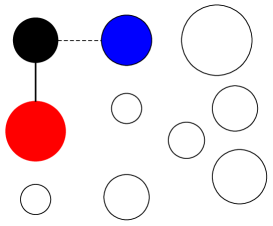
Figure 1: Illustration of the aggregation process with choice. Clusters are shown as disks, the bigger the disk the larger its size. The target cluster (black disk) and two potential merging partners (red and blue disks) are randomly drawn. The larger cluster (red disk) is chosen as the actual merging partner in the maximal choice case. In the minimal choice case, the smaller cluster (blue disk) is chosen.

We study kinetics of this aggregation process and focus on the long-time asymptotic behavior of the cluster-size density. Our reference frame is the well-understood behavior in the case of ordinary aggregation where the cluster-size density is purely exponential. We find that the density of the smallest clusters is anomalously large compared with typical-size clusters. This anomaly is not captured by the scaling function which characterizes the bulk of the density. We also find an interesting change in the shape of the size density. In addition to the overpopulation of smaller-than-typical clusters, there is also an overpopulation of larger-than-typical clusters. The small-size tail and the large-size tails are enhanced at the expense of moderate-size clusters. The enhancement of small clusters is easy to appreciate as it is a direct consequence of choosing the larger cluster. The enhancement of large clusters is an indirect, perhaps counter-intuitive, consequence of the aggregation rules.

We also study a few other implementations of choice. First, we consider the case where the smaller candidate cluster participates in the merging event. In this case, we observe an opposite change in the shape of the size density. Now, both the small-size tail and the large-size tail of the size density are suppressed, while the density of moderate-size clusters is enhanced. Second, we study aggregation processes where multiple candidates clusters are drawn and the maximal (or minimal) merges with the target cluster. In the maximal choice case, we find an interesting sequence of distinct scaling laws corresponding to the densities of the smallest clusters. Finally, we also investigate a symmetric implementation of choice where two candidate pairs are drawn at random and one of the pairs undergoes aggregation. We find that the changes in the shape of the size density, described above, are generic.

This paper is organized as follows. First, we briefly review ordinary aggregation, the most basic process where the merging clusters are chosen at random (Sec. II). Next, we introduce the notion of choice by considering the case where the larger of two randomly-selected clusters merges with another randomly-selected cluster. From the rate equation for the cluster-size density, we obtain the density of the smallest cluster, the small-size tail of the density, as well as the large-size tail of the density (Sec. III). We also detail results of our numerical simulations to gain insights into the entire size density. We apply the same theoretical tools to the case where the smaller of the two candidate clusters undergoes merger (Sec. IV), and to the case where multiple candidates clusters are drawn (Sec. V). In Sect. III–V the choice is implemented asymmetrically as the target cluster was selected from the outset. In Sec. VI, we introduce a symmetric implementation of choice where two pairs of clusters are chosen and only one of these pairs undergoes aggregation. We conclude in section VII and provide several technical details in the Appendices.

II Ordinary Aggregation

In ordinary aggregation, two clusters are chosen at random and merge to form a larger cluster Ald99 ; FL03 ; book . This basic process can be generalizes to model polymerization bk , condensation yo , chemotaxis sf , and random structures bk1 ; aal . Symbolically, we may represent the merger process as $i,j\to i+j$ where the aggregation rate is independent of cluster mass. The elementary aggregation step is repeated indefinitely. Initially, the system consists of identical particles whose mass can be set to unity. We tacitly take the thermodynamic limit, that is, assume that the initial number of particles is infinite.

Two clusters participate in each aggregation event and the number of clusters declines by one. Hence, the total cluster density $c(t)$ obeys the rate equation

$$\frac{dc}{dt}=-c^{2}\,.$$ (1)

Without loss of generality, we set the merging rate unity. Solving (1) subject to the initial condition $c(0)=1$ yields

$$c(t)=(1+t)^{-1}.$$ (2)

In the long-time limit we have $c\simeq t^{-1}$. (In our notations $a\sim b$ indicates the ratio $a/b$ approaches a constant when $t\to\infty$, while $a\simeq b$ indicates that the ratio approaches unity.)

Let $c_{k}(t)$ be the density of clusters of mass $k$ at time $t$. This quantity obeys the master equation

$$\frac{dc_{k}}{dt}=\sum_{i+j=k}c_{i}c_{j}-2c\,c_{k}\,.$$ (3)

By summing (3) we can verify that the density $c=\sum_{k}c_{k}$ obeys (1). The mass density $M=\sum_{k}k\,c_{k}$ is conserved $dM/dt=0$, as also follows from (3).

We shall consider the mono-disperse initial condition

$$c_{k}(0)=\delta_{k,1}\,.$$ (4)

We note that it suffices to use (4), because the asymptotic behavior is universal as long as the initial density decays rapidly with mass. The density of the smallest clusters, monomers, obeys $dc_{1}/dt=-2cc_{1}$, from which $c_{1}(t)=(1+t)^{-2}$. The monomer density decays more rapidly than the overall density, $c_{1}\simeq t^{-2}$. Starting from (4), the cluster-size density remains purely exponential

$$c_{k}(t)=\frac{t^{k-1}}{(1+t)^{k+1}}\,,$$ (5)

throughout the evolution.

Using mass conservation and the density decay (2) alone, we can deduce the average cluster size $\langle k\rangle=M/c$ or $\langle k\rangle=1+t$. In the long time-limit, the size distribution attains the scaling form

$$c_{k}(t)\simeq t^{-2}F(kt^{-1})\,.$$ (6)

This form reflects the linear growth of the typical mass $k\sim t$. According to the density decay $c\simeq t^{-1}$ and mass conservation, $M=1$, the scaling function must satisfy two constraints:

$$\int_{0}^{\infty}dx\,F(x)=1,\qquad\int_{0}^{\infty}dx\,x\,F(x)=1\,.$$ (7)

For ordinary aggregation Eq. (5) implies that the scaling function is purely exponential, $F(x)=e^{-x}$, a behavior that holds for any (rapidly decaying) initial condition.

Ordinary aggregation provides a useful reference point for our study. Throughout this study the density satisfies (1), and mass is certainly conserved. Moreover, the size density generally follows the scaling form (6), with the scaling function satisfying the constraints (7).

III Maximal Choice

We now incorporate choice while preserving most features of ordinary aggregation. In particular, aggregation remains a binary process with two clusters joining to form one larger cluster (Fig. 1). One cluster with size $i$ is selected at random, and it is certain to participate in the aggregation process. The aggregation partner is selected as the larger of two, randomly selected clusters of sizes $j_{1}$ and $j_{2}$. Schematically,

$$i,j_{1},j_{2}\to i+{\rm max}(j_{1},j_{2}),~{}{\rm min}(j_{1},j_{2})\,.$$ (8)

We reiterate that while three clusters are drawn, only two undergo aggregation. Mass is of course conserved and we consider the mono-disperse initial condition (4).

As in ordinary aggregation, two clusters are lost in each aggregation event and one new cluster is formed. Hence, the total density obeys (1), and it decays according to (2). Consequently, the growth of the typical mass as well as the scaling form (6) with the constraints (7) hold.

The cluster-size density obeys the master equation

$$\frac{dc_{k}}{dt}=c^{-1}\!\!\sum_{i+j=k}c_{i}\left(g_{j}^{2}-g_{j-1}^{2}\right)-c\,c_{k}-\left(g_{k}^{2}-g_{k-1}^{2}\right).$$ (9)

Here, $g_{k}=\sum_{l\leq k}c_{l}$ is the cumulative size density, namely, the density of clusters with size smaller than or equal to $k$. The gain term has the same convolution structure as (3) with one density corresponding to the target cluster and another density corresponding to the larger of the two candidate clusters. The quantity $g_{k}^{2}-g_{k-1}^{2}$ is proportional to the probability that the largest of two randomly selected clusters has size $k$, and the multiplicative constant $c^{-1}$ ensures proper normalization. There are two loss terms. The first represents the target cluster, and the second accounts for the selected cluster. One can verify that the total cluster density obeys (1).

Throughout this study, we repeatedly make the transformations

$$C_{k}=\frac{c_{k}}{c}\qquad\text{and}\qquad\tau=\ln(1+t).$$ (10)

The distribution $C_{k}$ is normalized, $\sum_{k}C_{k}=1$, and it represents the fraction of clusters of size $k$. It is also convenient to introduce the time variable $\tau$ which satisfies $dc/dt=1/c$. With the transformations (10), the first loss term in (9) is eliminated, and we arrive at

$$\frac{dC_{k}}{d\tau}=\sum_{i+j=k}C_{i}\left(G_{j}^{2}-G_{j-1}^{2}\right)-\left(G_{k}^{2}-G_{k-1}^{2}\right)\,.$$ (11)

Here $G_{k}=\sum_{l\leq k}C_{l}$ is the cumulative size distribution, the fraction of clusters with size not exceeding $k$.

For monomers, $k=1$, we have $dC_{1}/d\tau=-C_{1}^{2}$ and since $C_{1}(0)=1$, then $C_{1}(\tau)=(1+\tau)^{-1}$. In terms of the actual time variable, the density of monomers reads

$$c_{1}(t)=[(1+t)+(1+t)\ln(1+t)]^{-1}\,.$$ (12)

The asymptotic behavior $c_{1}\simeq(t\ln t)^{-1}$ represents a substantial enhancement over the monomer density $c_{1}\simeq t^{-2}$ for ordinary aggregation. As expected, monomers become populous because they are least likely to participate in the aggregation process (8).

A more elaborate calculation (see Appendix A) gives the density of dimers:

$$c_{2}=e^{-\tau}u^{3}\,\frac{I_{0}(2)K_{0}(2\,u)-K_{0}(2)I_{0}(2\,u)}{I_{0}(2)K_{1}(2\,u)+K_{0}(2)I_{1}(2\,u)}\,.$$ (13)

Here $I_{\nu}$ and $K_{\nu}$ are the modified Bessel functions with index $\nu$, and $u=(1+\tau)^{-1/2}$. Using the asymptotic relations, $K_{0}(2u)\simeq\ln(1/u)$ and $K_{1}(2u)\simeq(2u)^{-1}$ when $u\to 0$, we find the asymptotic decay

$$c_{2}(t)\simeq\frac{1}{t}\,\frac{\ln(\ln t)}{(\ln t)^{2}}\,.$$ (14)

The dimer density is much smaller the monomer density, $\frac{c_{2}}{c_{1}}\simeq\frac{\ln(\ln t)}{\ln t}$ when $t\gg 1$. In comparison with ordinary aggregation where $c_{2}\simeq t^{-2}$, the dimer density (14) is substantially larger, however.

For trimers and other finite clusters, $k\geq 3$, we can obtain the leading asymptotic behavior. As for monomers and dimers, the loss rate in (11) dominates. Furthermore, since $C_{1}\gg C_{2}$ in the asymptotic regime, the dominant term in Eq. (11) involves the monomer fraction,

$$\frac{dC_{k}}{d\tau}\simeq-2C_{1}C_{k}\,.$$ (15)

We now substitute the asymptotic behavior $C_{1}\simeq\tau^{-1}$, and immediately obtain $C_{k}\sim\tau^{-2}$. In terms of the physical time variable

$$c_{k}(t)\sim\frac{1}{t}\,\frac{1}{(\ln t)^{2}}$$ (16)

for $3\leq k\ll t$. Hence, $c_{1}\gg c_{2}\gg c_{k}$ when $k\geq 3$. The ratio $\frac{c_{2}}{c_{3}}\sim\ln(\ln t)$ diverges with time, but very slowly.

In summary, equations (12), (13), and (16) show that there are three distinct scaling laws for small clusters

$$c_{k}\sim\begin{cases}\frac{1}{t}\,\frac{1}{(\ln t)}&k=1\cr\frac{1}{t}\,\frac{\ln(\ln t)}{(\ln t)^{2}}&k=2\cr\frac{1}{t}\,\frac{1}{(\ln t)^{2}}&k\geq 3.\cr\end{cases}$$ (17)

As a consequence of choice, there is a strong enhancement of small clusters compared to ordinary aggregation. Further, three different decay laws characterize the density of monomers, dimers, and clusters of mass $3\leq k\ll t$. As we show below, the scaling function underlying the cluster-size density captures $c_{k}$ with $k\geq 3$.

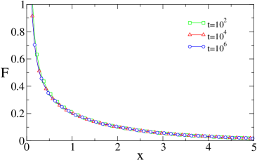
Figure 2: The scaling function $F(x)$ in the maximal choice model. Shown is $F(x)\equiv t^{2}c_{k}(t)$ versus the scaling variable $x=k/t$ at three different times.

Our numerical simulations (see Fig. 2) confirm that the cluster-size density adheres to the scaling form (6): in terms of the properly normalized cluster size $x=k/t$, the size density has a universal shape in the asymptotic regime. The scaling function $F(x)$ satisfies the integro-differential equation

$$\frac{d[xF(x)]}{dx}+\int_{0}^{x}dyF(x-y)\frac{d\Phi^{2}(y)}{dy}-\frac{d\Phi^{2}(x)}{dx}=0\,.$$ (18)

Here $\Phi(x)=\int_{0}^{x}dyF(y)$ is the fraction of clusters with size smaller than $x=k/t$ in the long-time limit. To obtain (18) we simply substitute (6) into the rate equation (11). The two nonlinear terms in (18) correspond to the two nonlinear terms in (11).

First, we consider statistics of small clusters. As mentioned above, the convolution term, which corresponds to generation of larger clusters from smaller clusters through aggregation, is negligible. Keeping only the leading terms when $x\ll 1$, we get

$$\frac{d}{dx}\left[x\,F-\Phi^{2}(x)\right]=0\,.$$ (19)

Hence $xF=\Phi^{2}$, or alternatively $x\Phi^{\prime}=\Phi^{2}$. Solving this differential equation yields $\Phi=[\ln(1/x)]^{-1}$ leading to the asymptotic behavior

$$F(x)\simeq\frac{1}{x}\,\frac{1}{[\ln(1/x)]^{2}}\,$$ (20)

as $x\to 0$. This form is consistent with the cluster density (16), and it specifies the proportionality constant: $c_{k}\simeq k^{-1}\,[t\,(\ln t)^{2}]^{-1}$. The diverging small-$x$ tail of the scaling function does not capture the anomalous populations of monomers and dimers (see Fig. 2).

Next, let us consider statistics of large clusters. In the limit $x\gg 1$, the convolution term is dominant, and the governing equation (18) becomes

$$xF^{\prime}(x)+2\int_{0}^{x}dyF(y)F(x-y)=0\,.$$ (21)

Here, we also assumed $xF^{\prime}\gg F$ which can be justified a posteriori. Equation (21) is essentially the same as in ordinary aggregation, and therefore, the tail is exponential:

$$F(x)\simeq\frac{\alpha}{2}e^{-\alpha x}$$ (22)

when $x\to\infty$. Our numerical simulations confirm this exponential asymptotic decay (see Fig. 3) with the constant $\alpha=0.57\pm 0.01$.

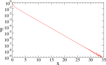
Figure 3: The large-size tail of the scaling function $F(x)$ showing the exponential decay (22).

The tail (20) shows that the density of small clusters is enhanced compared with ordinary aggregation: $F(x)\gg e^{-x}$ when $x\to 0$. This is an expected consequence of choice — very small clusters are less likely to participate in aggregation, so their population is enhanced. Remarkably, the same holds for large clusters — since $\alpha<1$, the large-size tail (22) is enhanced compared with ordinary aggregation, $F(x)\gg e^{-x}$ when $x\to\infty$. This is an indirect consequence of choice — somehow very large clusters are “shielded” from aggregation.

Figure (4) compares aggregation with choice with ordinary aggregation, and it demonstrates that there are three regimes of behavior, as the normalized scaling function $e^{x}F(x)$ is non-monotonic. Small clusters with size $x<x_{1}$ are overpopulated compared with ordinary aggregation. Large clusters with size $x>x_{2}$ are also overpopulated compared with ordinary aggregation. The conservation laws (7) dictate that clusters of moderate sizes $x_{1}<x<x_{2}$ must be underpopulated. Hence, introducing choice alters the shape of the size density.

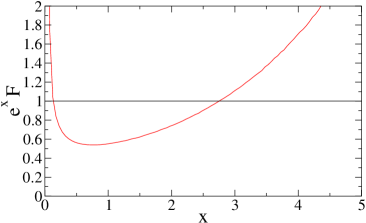
Figure 4: The normalized scaling function $e^{x}\,F(x)$ versus the scaling variable $x$. Also shown for reference is the unit constant corresponding to the ordinary aggregation case.

Monte Carlo simulations of aggregation processes are rather straightforward when the aggregation rate is uniform as is the case of the merging rule (8) and other rules studied in this paper. Initially, the system consists of $N_{0}$ identical particles with unit mass. In each aggregation event, three distinct particles are selected at random. One of these particles is designated as the target particle, and it merges with the larger of the remaining two particles. When $N_{0}$ is large, the overall density (2) specifies time as $t\equiv N_{0}/N$ where $N$ is the number of remaining aggregates. The simulation results presented throughout this paper were obtained using $N_{0}=10^{8}$, and an average over roughly $10^{5}$ independent realizations.

IV Minimal Choice

We now consider the complementary case where the target cluster merges with the smaller of the two candidate clusters (see also Fig. 1) according to the scheme

$$i,j_{1},j_{2}\to i+{\rm min}(j_{1},j_{2}),~{}{\rm max}(j_{1},j_{2})\,.$$ (23)

As in maximal choice mass is conserved, and the total density decays according to (2).

The size-density $c_{k}(t)$ satisfies the master equation

$$\frac{dc_{k}}{dt}=c^{-1}\!\!\!\sum_{i+j=k}c_{i}\left(h_{j}^{2}-h_{j+1}^{2}\right)-c\,c_{k}-\left(h_{k}^{2}-h_{k+1}^{2}\right)$$ (24)

subject to (4). The quantity $h_{k}=\sum_{l\geq k}c_{l}$ is the density of clusters of size larger than or equal to $k$. The cumulative distributions $h_{k}$ and $g_{k-1}$ appearing in (9) are complimentary: $g_{k-1}+h_{k}=c$ for all $k\geq 1$. As in Eq. (9), the first loss term in Eq. (24) corresponds to the target cluster and the second, to the selected cluster. The quantity $h_{k}^{2}-h_{k+1}^{2}$ is proportional to the probability that the selected cluster has size $k$. By summing (24), we can verify that the density satisfies (1).

In terms of the modified time variable $\tau$, the size distribution $C_{k}$ satisfies

$$\frac{dC_{k}}{d\tau}=\sum_{i+j=k}C_{i}\left(H_{j}^{2}-H_{j+1}^{2}\right)-\left(H_{k}^{2}-H_{k+1}^{2}\right).$$ (25)

Here $H_{k}=\sum_{l\geq k}C_{l}$. We note that $G_{k}+H_{k+1}=1$ and $H_{1}=1$ at all times. The initial condition (4) becomes $C_{k}(0)=\delta_{k,1}$.

According to (25) the density of monomers satisfies $\frac{dC_{1}}{d\tau}=C_{1}^{2}-2C_{1}$, with $C_{1}(0)=1$. This Bernoulli equation is solved to yield $C_{1}(\tau)=2/(1+e^{2\tau})$. In terms of the original time variable, the density of monomers reads

$$c_{1}(t)=\frac{2}{(1+t)+(1+t)^{3}}\,.$$ (26)

In the long-time limit we have $c_{1}(t)\simeq 2\,t^{-3}$, whereas in ordinary aggregation $c_{1}(t)\simeq t^{-2}$. Monomers are most likely to participate in the aggregation process (23), and consequently, they decay rapidly.

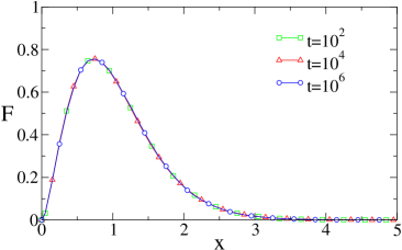
Figure 5: The scaling function $F(x)$ in the minimal choice model. Shown is $F(x)\equiv t^{2}c_{k}(t)$ versus the scaling variable $x=k/t$ at three different times.

One can also obtain the exact expression for the dimer density (see Appendix A)

$$c_{2}=\frac{(e^{-\tau}\,v)^{3}}{8}\,\frac{J_{0}(2)Y_{0}(v)-Y_{0}(2)J_{0}(v)}{Y_{0}(2)J_{1}(v)-J_{0}(2)Y_{1}(v)}\,.$$ (27)

Here $J_{\nu}$ and $Y_{\nu}$ are the Bessel functions with index $\nu$ and $v=[8/(1+e^{-2\tau})]^{-1/2}$. Asymptotically, the dimer density decays according to $c_{2}(t)\simeq A_{2}\,t^{-3}$ with the prefactor

$$A_{2}=\sqrt{8}\,\,\frac{J_{0}(2)Y_{0}(\sqrt{8})\!-\!Y_{0}(2)J_{0}(\sqrt{8})}{Y_{0}(2)J_{1}(\sqrt{8})\!-\!J_{0}(2)Y_{1}(\sqrt{8})}\,$$ (28)

or $A_{2}=3.878012\cdots$. In contrast with the behavior (17), the ratio $c_{2}/c_{1}$ now approaches a nontrivial constant.

For finite but small $k$, the loss rate in (11) dominates. By using $H_{k}-H_{k+1}=C_{k}$ we have $dC_{k}/d\tau\simeq-2C_{k}$, and therefore $C_{k}(\tau)\sim e^{-2\tau}$. In general, the density of small clusters decays algebraically,

$$c_{k}(t)\simeq A_{k}\,t^{-3}\,,$$ (29)

for finite $k\ll t$. As expected, small clusters are suppressed due to choice. In contrast with maximal choice, however, there are no anomalies associated with monomers or with dimers, and a single scaling law characterizes small clusters. As shown below, the decay (29) is captured by the scaling function $F(x)$.

Our numerical simulations confirm that once size is rescaled by the typical size, $k\simeq t$, the size distribution becomes universal in the long-time limit (see Fig. 5). By substituting the scaling ansatz (6) into the governing equation (24), we find that the scaling function obeys

$$\frac{d[xF(x)]}{dx}-\int_{0}^{x}dyF(x-y)\frac{d\Psi^{2}(y)}{dy}+\frac{d\Psi^{2}(x)}{dx}=0\,.$$ (30)

Here $\Psi(x)=\int_{x}^{\infty}dyF(y)$ is the fraction of clusters of size larger than $x=k/t$. Once again, the scaling function obeys the two constraints in (7).

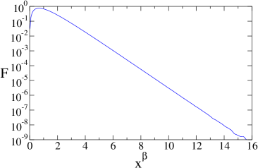
Figure 6: The large-$x$ tail of the scaling function $F(x)$ showing the super-exponential decay (34) with $\beta\cong 1.26749$.

First, we discuss statistics of small sizes. The convolution term is negligible when $x\ll 1$ and using $\Psi^{\prime}(x)=-F(x)$ we get $xF^{\prime}(x)=F(x)$. Therefore the scaling function is linear (see Fig. 5)

$$F(x)\sim x\,,$$ (31)

in the limit $x\to 0$. The linear behavior confirms (29), and further, it shows that $A_{k}\sim k$ for large but finite $k$. In contrast with maximal choice, the equation governing $F(x)$ is linear in the limit $x\to 0$, and determining the proportionality constant in $F(x)\simeq{\rm const.}\times x$ requires a full solution of the nonlinear equation (30).

Let us now consider the large-$x$ behavior. Since the convolution term is dominant in (30), we have

$$\frac{d[xF(x)]}{dx}+2\int_{0}^{x}dyF(x-y)\frac{d\Psi^{2}(y)}{dy}=0$$ (32)

when $x\gg 1$. We anticipate (and justify a posteriori) a sharp decay of the scaling function. In this scenario, $\Psi(x)=\int_{y}^{\infty}dzF(z)\asymp F(y)$ and $-F^{\prime}(x)\asymp F(x)$. (We use the notation $A\asymp B$ to imply that the logarithms of $A$ and $B$ have the same asymptotic behavior, $\ln A\simeq\ln B$.) Further, we postulate that the integral in (32) is maximal at $y=\sigma\,x$, with $0<\sigma<1$, and therefore

$$F(x)\asymp F^{2}(\sigma\,x)F(x-\sigma\,x)\,.$$ (33)

Taking the logarithm of both sides we arrive at a linear functional equation $\ln F(x)=2\ln F(\sigma\,x)+\ln F(x-\sigma\,x)$ . This equation admits a simple family of algebraic solutions, $\ln F(x)\simeq-{\rm const}\times x^{\beta}$, or equivalently,

$$F(x)\asymp\exp\left(-{\rm const.}\times x^{\beta}\right)\,$$ (34)

with exponent $\beta>1$. The exponent $\beta$ and the parameter $\sigma$ are related via

$$2\sigma^{\beta}+(1-\sigma)^{\beta}=1\,.$$ (35)

An additional relation is needed to “select” $\beta$. Selection problems arise in the context of nonlinear partial differential equations van03 and nonlinear recurrences MK03 . Typically, the selection criterion is tied to an extremum, as is the case for velocity selection in traveling waves van03 . Guided by these examples, we postulate that $\beta$ is selected by the requirement that the quantity $\sigma\equiv\sigma(\beta)$, determined by Eq. (35), increases with maximal rate at the selected $\beta$, that is $d\sigma/d\beta$ is maximal. This extremum requirement specifies the selection criterion

$$\frac{d^{2}\sigma}{d\beta^{2}}=0\,.$$ (36)

Using equations (35) and (36) we obtain (see Appendix B for further details) $\beta\cong 1.26749$ and the corresponding $\sigma\cong 0.166453$. Our simulation results support this value, as shown in figure 6. The super-exponential tail for large $x$ is sufficiently sharp to provide an a posteriori justification to the assumptions made in deriving (35).

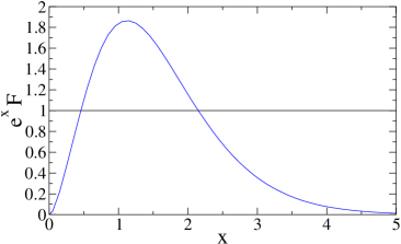
Figure 7: The normalized scaling function $e^{x}\,F(x)$ versus the scaling variable $x$. Also shown for reference is the unit constant, corresponding to the ordinary aggregation case.

The small-size tail (31) confirms that when the smaller of the two candidate clusters undergoes aggregation, the population of small clusters is suppressed. The large-size tail (34) is much steeper than exponential: $F(x)\ll e^{-x}$ for large $x$. Figure 7 compares the scaling function for minimal choice with ordinary aggregation. There are three regimes of behaviors: in the small mass range $x<x_{1}$ and in the large mass range $x>x_{2}$ the cluster-size density is underpopulated while in the intermediate size range $x_{1}<x<x_{2}$ the density is overpopulated. Hence, the effect on size density is the exact opposite of that found for the maximal case.

V Multiple Choice

In Sections III and IV we showed that choice between two alternatives significantly affects the size density. What happen if we allow choice between more than two alternatives? In the context of other models broder ; adler ; michael , the general conclusion was that multiple choice modifies the behavior only quantitatively. As we show below, introduction of multiple choice in aggregation has interesting consequences, including some quantitative changes.

V.1 Maximal Choice

We start with the maximal case, and introduce multiple choice as to preserves the binary nature of the aggregation process. As in section III, we choose a single target cluster along with $n$ candidate clusters. The target cluster merges with the largest of these $n$ clusters, while the rest of the $n-1$ clusters are not affected. This merger process preserves the total mass, and the total cluster density is given by (2).

The cluster-size density $c_{k}(t)$ obeys

$$\frac{dc_{k}}{dt}=\sum_{i+j=k}c_{i}\frac{g_{j}^{n}-g_{j-1}^{n}}{c^{n-1}}-c\,c_{k}-\frac{g_{k}^{n}-g_{k-1}^{n}}{c^{n-2}}\,,$$ (37)

where $g_{k}=\sum_{l\leq k}c_{l}$ is the cumulative density. The master equation (37) reduces to (3) and (11) when $n=1$ and $n=2$, respectively. The quantity $g_{k}^{n}-g_{k-1}^{n}$ is proportional to the probability that the selected cluster has size $k$. From (37) we can obtain the master equation governing the normalized cluster-size distribution $C_{k}=c_{k}/c$. Using the time variable $\tau=\ln(1+t)$ and $G_{k}=\sum_{l\leq k}C_{l}$ we get

$$\frac{dC_{k}}{d\tau}=\sum_{i+j=k}C_{i}\left(G_{j}^{n}-G_{j-1}^{n}\right)-\left(G_{k}^{n}-G_{k-1}^{n}\right).$$ (38)

The density of monomers satisfies $dC_{1}/d\tau=-C_{1}^{n}$, from which $C_{1}(\tau)=[1+(n-1)\tau]^{-1/(n-1)}$ . In terms of the physical time

$$c_{1}(t)=(1+t)^{-1}\left[1+(n-1)\ln(1+t)\right]^{-1/(n-1)}\,.$$ (39)

This decay represents an enhancement over ordinary aggregation.

For finite cluster size $k$, it is possible to proceed with asymptotic analysis of (11) and find $C_{k}\sim C_{1}^{k}$ for $k<n$ and $C_{k}\sim C_{1}^{n}$ for $k>n$. The three-tier asymptotic behavior (17) generalizes as follows

$$c_{k}(t)\sim\begin{cases}\frac{1}{t}\,\frac{1}{(\ln t)^{k/(n-1)}}&k<n\,,\\ \frac{1}{t}\,\frac{\ln(\ln t)}{(\ln t)^{n/(n-1)}}&k=n\,,\\ \frac{1}{t}\,\frac{1}{(\ln t)^{n/(n-1)}}&k>n\,.\end{cases}$$ (40)

Interestingly, there are $n$ distinct scaling laws that characterize the enhancement of small clusters. The density of monomers is the largest, the density of dimers is the next largest and so on. Thus, multiple choice leads to multiple anomalies in the cluster-size density.

The scaling function now obeys an integro-differential equation

$$\frac{d}{dx}\left[x\,F-\Phi^{n}(x)\right]+\int_{0}^{x}dy\,F(x-y)\frac{d\Phi^{n}(y)}{dy}=0$$ (41)

which generalizes (18). Here $\Phi(x)=\int_{0}^{x}dyF(y)$ is the fraction of clusters with size smaller than $x$. The tails of the scaling function are derived by repeating the steps leading to (20) and (22) to give

$$F(x)\simeq\begin{cases}\frac{1}{x}\,\frac{1}{[(n-1)\ln(1/x)]^{n/(n-1)}}&x\ll 1\,,\cr\frac{\alpha}{n}\exp(-\alpha\,x)&x\gg 1\,.\end{cases}$$ (42)

The small-$x$ tail captures the behavior of clusters with size $n<k\ll t$, and the logarithmic divergence reflects the relative abundance of small clusters due to choice. The divergence in the limit $x\to 0$ becomes weaker and weaker as $n$ grows. Based on the behavior in the case $n=2$ we anticipate that $\alpha<1$ in general, and that there is also an increase in the density of large clusters compared with ordinary aggregation.

V.2 Minimal choice

In the complementary case of minimal choice, the target cluster merges with the smallest of $n$ candidate clusters. In terms of the modified time variable $\tau$, the cluster-size distribution $C_{k}$ satisfies

$$\frac{dC_{k}}{d\tau}=\sum_{i+j=k}C_{i}\left(H_{j}^{n}-H_{j+1}^{n}\right)-\left(H_{k}^{n}-H_{k+1}^{n}\right),$$ (43)

with $H_{k}=\sum_{l\geq k}C_{l}$. The master equation (43) generalizes (25) which corresponds to the case $n=2$.

For finite and small $k$, the leading asymptotic behavior is purely algebraic as in (29)

$$c_{k}(t)\simeq A_{k}t^{-n-1}\,.$$ (44)

This behavior readily follows from (43) by noting that the dominant term is linear, that is, $dC_{k}/d\tau\simeq-nC_{k}$. Hence, $C_{k}\sim e^{-n\tau}$ and (44) follows. The small-cluster densities (44) confirm that small clusters are suppressed when the minimal cluster is chosen for aggregation.

For monomers, it is possible to obtain the constant $A_{1}$ analytically. The monomer concentration obeys $dC_{1}/d\tau=(1-C_{1})^{n}-1$, from which

$$\int_{C_{1}}^{1}\frac{dv}{1-(1-v)^{n}}=\tau\,.$$ (45)

One can evaluate this integral in the asymptotic limit where the lower limit of the integration vanishes to confirm the decay (44). Moreover, the general expression for the amplitude is

$$A_{1}=\exp\left\{\int_{0}^{1}dv\left[\frac{n}{1-(1-v)^{n}}-\frac{1}{v}\right]\right\}\,.$$ (46)

The amplitudes $A_{1}$ for $n\leq 6$ are listed in Appendix C.

$n$	2	20	200	2000	20000
$\beta$	1.26749	2.14474	3.05326	3.99381	4.9607

Table 1: The exponent $\beta$ obtained by solving (49) and (72) for $n=2,20,200,2000,20000$.

The scaled mass distribution function $F(x)$ satisfies the general version of (30),

$$\frac{d[xF(x)]}{dx}-\int_{0}^{x}dyF(x-y)\frac{d\Psi^{n}(y)}{dy}+\frac{d\Psi^{n}(x)}{dx}=0\,.$$ (47)

Here, $\Psi(x)=\int_{x}^{\infty}dyF(y)$. By repeating the steps leading to the tails (31) and (34), we obtain the leading asymptotic behaviors

$$F(x)\sim\begin{cases}x^{n-1}&x\ll 1\,,\cr\exp\left(-{\rm const.}\times x^{\beta}\right)&x\gg 1\,.\end{cases}$$ (48)

The small-$x$ tail is consistent with (44) and additionally, it indicates that $A_{k}\sim k^{n-1}$ when $1\ll k\ll t$. The suppression of small clusters becomes stronger and stronger as $n$ grows. In this sense, choice provides a mechanism for controlling the size distribution. The large-$x$ tail is steeper than an exponential, and the exponent $\beta$ is determined by

$$n\sigma^{\beta}+(1-\sigma)^{\beta}=1\,,$$ (49)

along with the selection criterion (36). Appendix B provides additional details on the derivation of $\beta$, and Table I lists several values of $\beta$. Since $\beta$ increases with $n$, suppression of large clusters becomes stronger with increasing $n$.

VI Symmetric Choice

In Sects. III–V we implemented choice asymmetrically: One cluster was selected from the outset, while its merging partner was chosen from two or more alternatives. Asymmetric choice can arise, for example, in network growth when a new node considers a few provisional links, and then implements only one of these links according to a pre-determined selection criterion. We recall that the Achlioptas process is symmetric ASS , namely two pairs of nodes are randomly chosen and the link between nodes from one pair is made. This motivates one to introduce choice using the very same procedure where clusters from one of the two randomly selected pairs merge.

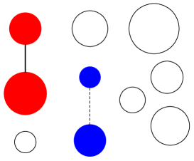
Figure 8: Illustration of aggregation with symmetric choice. Two pairs (two red disks and two blue disks) are randomly drawn. The pair with bigger combined size (red pair) is chosen in the maximal choice case. In the minimal choice case, the pair with smaller combined size (blue pair) is chosen.

VI.1 Maximal choice

In the symmetric version of aggregation with choice, we choose two pairs of clusters with sizes $i_{1},j_{1}$ and $i_{2},j_{2}$. All four clusters are chosen randomly. Without loss of generality, we assume that $i_{1}+j_{1}\geq i_{2}+j_{2}$. Under maximal choice, the pair with the larger total mass undergoes aggregation (see Fig. 8):

$$i_{1},j_{1},i_{2},j_{2}\to i_{1}+j_{1},i_{2},j_{2}\,.$$ (50)

Hence, the selection criterion is such that the total size of the resulting aggregate is maximized. In the Achlioptas process ASS , in contrast, the selection criterion is different, e.g. the product of the sizes can be sought to be maximal, so that the choice (50) is made if $i_{1}\cdot j_{1}\geq i_{2}\cdot j_{2}$.

The aggregation process (50) involves four clusters, and the corresponding master equation governing the cluster-size density is quartic

$$c^{2}\,\frac{dc_{k}}{dt} = \sum_{i+j=k}c_{i}c_{j}\left(2\sum_{k^{\prime}<k}c_{i^{\prime}}c_{j^{\prime}}+\sum_{k^{\prime}=k}c_{i^{\prime}}c_{j^{\prime}}\right)$$

$$- 2c_{k}\Bigg{(}2\sum_{k^{\prime}<k+j}c_{j}c_{i^{\prime}}c_{j^{\prime}}+\sum_{k^{\prime}=k+j}c_{j}c_{i^{\prime}}c_{j^{\prime}}\Bigg{)}\,,$$

with $k^{\prime}=i^{\prime}+j^{\prime}$. There are two gain terms and two loss terms. The first gain term accounts for the case where the two pairs have different total size, and the second gain term, for the complementary case of equal total size. The two loss terms are similarly ordered.

Our numerical simulations show that the scaling function $F(x)$ maintains the same qualitative features as in the asymmetric case. Figure 9 shows that the scaling function $F(x)$ diverges at small-$x$, thereby indicating an overpopulation of small clusters. Similarly, figure (10) which shows the normalized scaling function $e^{x}F(x)$ demonstrates that there is also an overpopulation of large clusters. Once again, there are three size regimes, and at intermediate sizes, the density is suppressed.

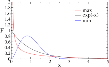
Figure 9: The scaling function $F(x)$ versus the scaling variable $x$ for maximal choice, ordinary aggregation, and minimal choice.

By substituting (6) into (VI.1), we see that the scaling function obeys

$$0=xF^{\prime}(x) + 2F(x)+2\phi(x)\int_{0}^{x}dy\,F(y)F(x-y)$$ (52)

$$- 4F(x)\int_{0}^{\infty}dy\,F(y)\phi(x+y)\,.$$

In deriving this equation we took into account that the second gain term and the second loss term which correspond to the case where $i_{1}+j_{1}=i_{2}+j_{2}$ are asymptotically negligible. The function $\phi(z)$ appearing in (52) is the shorthand notation for the following integral

$$\phi(z)=\iint_{x^{\prime}+y^{\prime}<z}dx^{\prime}dy^{\prime}F(x^{\prime})F(y^{\prime})\,.$$ (53)

The scaling function is subject to the normalization (7).

At small sizes, the convolution term in (52) is negligible and it simplifies to $xF^{\prime}=(\gamma-2)F$ with

$$\gamma=4\int_{0}^{\infty}dy\,F(y)\phi(y)\,.$$ (54)

The scaling function is therefore algebraic, $F(x)\sim x^{\gamma-2}$, when $x\ll 1$. This algebraic behavior implies the algebraic decay

$$c_{k}\sim t^{-\gamma}$$ (55)

for finite $k\ll t$. Indeed, it is possible to derive (55) with (54) directly from the master equation (VI.1) together with the scaling form (6). The behavior (55) also holds for monomers, and there is no longer an anomaly associated with minimal clusters.

The exponent $\gamma$, which according to (54) requires full knowledge of $F(x)$, appears to be nontrivial. Our numerical simulations yield $\gamma=1.25\pm 0.01$ (Fig. 11). If we ignore the logarithmic correction in (20), then the corresponding value for the asymmetric case is $\gamma=1$. We have not determined $\gamma$ analytically, but in Appendix D we derive the bounds

$$1\leq\gamma<\frac{4}{3}\,.$$ (56)

According to these bounds, the scaling function diverges in the limit $x\to 0$ (see Fig. 9).

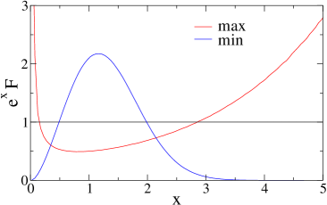
Figure 10: The normalized scaling function $e^{x}\,F(x)$ versus the scaling variable $x$. Shown are the cases of maximal choice, ordinary aggregation, and ordinary aggregation.

At large sizes, the convolution term dominates and $\phi\to 1$, so that Eq. (52) simplifies to (21). Consequently, $F(x)$ decays exponentially according to (22). Numerically, we find the decay constant $\alpha=0.53\pm 0.01$, which is slightly smaller than the value $\alpha=0.57\pm 0.01$ for the asymmetric case. The extremal behaviors of the scaling function are therefore

$$F(x)\sim\begin{cases}x^{\gamma-2}&x\to 0,\\ e^{-\alpha x}&x\to\infty.\\ \end{cases}$$ (57)

Thus, many of the features obtained for aggregation with asymmetric choice extend to aggregation with symmetric choice. The density of very small and very large clusters are enhanced at the expense of moderate-size clusters. The normalized size density again diverges at small sizes, and interestingly, this divergence is characterized by a nontrivial exponent. There is one difference between the two cases, however. The scaling function captures the asymptotic behavior at all scales and there is no anomaly associated with small clusters.

VI.2 Minimal choice

We now consider the complementary case where the pair with the minimal total mass undergoes aggregation. Aggregation proceeds according to (50) except that now $i_{1}+j_{1}\leq i_{2}+j_{2}$. Repeating the above analysis one finds that the scaling function satisfies

$$0=xF^{\prime}(x) + 2F(x)+2\psi(x)\int_{0}^{x}dyF(y)F(x-y)$$ (58)

$$- 4F(x)\int_{0}^{\infty}dyF(y)\psi(x+y)\,.$$

This equation differs from (52) in that $\phi(y)$ is replaced by the complementary integral

$$\psi(y)=\iint_{x^{\prime}+y^{\prime}>y}dx^{\prime}dy^{\prime}F(x^{\prime})F(y^{\prime})\,,$$ (59)

so that $\psi(y)+\phi(y)=1$ for all $y$. Asymptotic analysis of equation (58) yields

$$F(x)\sim\begin{cases}x^{\gamma-2}&x\to 0,\\ e^{-{\rm const.}\times x^{2}}&x\to\infty.\\ \end{cases}$$ (60)

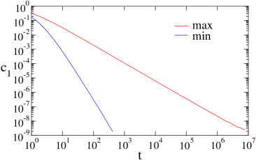
Figure 11: The monomer density $c_{1}(t)$ versus time $t$ for symmetric aggregation with maximal and minimal choice.

The small-$x$ behavior is characterized by the nontrivial exponent $\gamma$ which is given by the analog of (54)

$$\gamma=4\int_{0}^{\infty}dy\,F(y)\psi(y)\,.$$ (61)

Numerically, we find the value $\gamma=3.5\pm 0.1$ (Fig. 11), which is somewhat larger than the value $\gamma=3$ above. Hence, the suppression of small clusters becomes stronger under the symmetric aggregation process (50). In Appendix D, we obtain the bounds

$$\frac{8}{3}\leq\gamma\leq 4\,.$$ (62)

The small-$x$ tail (60) implies that the density of small clusters decay algebraically with time according to (55).

To estimate the large-size tail, we first note that for a sharply-decaying $F(x)$, the integrand in (59) is maximal at $x^{\prime}=y^{\prime}=x/2$, and as a result $\psi(x)\asymp F^{2}(x/2)$. Following this reasoning, we estimate that the convolution term in (58) behaves as $F^{2}(x/2)$. For large $x$, the derivative term and the convolution term dominate, and balancing these two terms gives

$$-xF^{\prime}(x)\asymp F^{4}(x/2)\,.$$ (63)

We now substitute the super-exponential form (34) and obtain $1=4/2^{\beta}$ from which we deduce $\beta=2$ leading to the Gaussian tail in (60). Compared with the value $\beta=1.26749$ in the asymmetric case, we deduce that the tail is now sharper.

Figures 9 and 10 compare the scaling function $F(x)$ with the exponential decay $e^{-x}$ which corresponds to ordinary aggregation. As in the case of symmetric aggregation, the populations of very small and very large clusters are suppressed, while the population of intermediate clusters is enhanced. we conclude that the qualitative behavior of the size density for aggregation with symmetric and asymmetric choice are similar.

VII Conclusions

In summary, we generalized the most basic aggregation process to include choice. In our implementation, several clusters are drawn at random, and two clusters merge while the rest are not affected. The merging clusters are chosen in a way that maximizes or minimizes the aggregate size. We considered several versions and found a number of common features. In all cases, the size density adheres to standard scaling, in contrast with some aggregation processes in which scaling is violated (see e.g. ASP82 ; HE84 ; LR87 ; MKR03 .)

In general, introduction of choice changes the shape of the cluster-size distribution. When the merger maximizes the size of the final aggregate, the small-size tail of the distribution is enhanced because small clusters are less likely to undergo aggregation. Surprisingly, the large-size tail of the distribution is also enhanced. The opposite effect emerges when the merging clusters minimize the aggregate size. These qualitative features are general, and hold regardless of the number of clusters involved in the aggregation process.

We found a number of interesting features for aggregation with choice. In the asymmetric version with maximal choice, the scaling function does not capture the entire size density. In particular, when $n$ clusters are involved in the aggregation process, there are $n$ distinct scaling laws that characterize the density of monomers, dimers, up to $n$-mers. The population of these small clusters is anomalously large compared with that of typical clusters. In the asymmetric version with minimal choice, the large-$x$ tail is super-exponential $F(x)\sim\exp[-{\rm const.}\times x^{\beta}]$, and it is governed by a nontrivial exponent $\beta>1$. This exponent is selected from a spectrum of possible values according to a principle that is reminiscent of velocity selection in nonlinear traveling waves.

One model with symmetric choice which would be interesting to explore is the following: Pick up randomly three clusters and merge two of them, e.g. the smallest or the largest. We analyzed our models only in the mean-field case, and another extension is to aggregation in finite spatial dimensions. For instance, clusters may occupy a single lattice site, and hop to adjacent sites with the same mass-independent rate, and when three clusters occupy the same site, two of them, say the smallest, merge. The third (largest) cluster thus plays a role of a catalyst. This toy model is inspired by living matter, as most biological processes involve a catalyst.

We acknowledge support from US-DOE grant DE-AC52-06NA25396 (EB).

Appendix A The fraction of dimers $C_{2}$

For maximal choice, the fraction of dimers obeys

$$\frac{dC_{2}}{d\tau}=C_{1}^{3}+C_{1}^{2}-(C_{1}+C_{2})^{2}\,.$$ (64)

Using $C_{1}=1/(1+\tau)$, we obtain the Riccati equation

$$\frac{dC_{2}}{d\tau}=-C_{2}^{2}-\frac{2}{1+\tau}C_{2}+\frac{1}{(1+\tau)^{3}}\,.$$ (65)

To find the solution we first linearize the first-order nonlinear differential equation (65) by making the transformation $C_{2}=-[2u^{3}f(u)]/f^{\prime}(u)$ with $u=(1+\tau)^{-1/2}$. The quantity $f(u)$ obeys the Bessel equation, and thereby, we arrive at the dimer fraction

$$C_{2}=u^{3}\,\frac{I_{0}(2)K_{0}(2\,u)-K_{0}(2)I_{0}(2\,u)}{I_{0}(2)K_{1}(2\,u)+K_{0}(2)I_{1}(2\,u)}.$$ (66)

For minimal choice, we have

$$\frac{dC_{2}}{d\tau}=2C_{1}^{2}+C_{2}^{2}-C_{1}^{3}+2C_{1}C_{2}-2C_{2}\ .$$ (67)

We now write

$$C_{2}=e^{-2\tau}U_{2}(T),\quad T=e^{-2\tau}.$$ (68)

Recalling that $C_{1}=2/(1+e^{2\tau})=2T/(1+T)$ and using (68) we recast (67) into

$$\frac{dU_{2}}{dT}=-\frac{1}{2}U_{2}^{2}-\frac{2}{1+T}\,U_{2}-\frac{4}{(1+T)^{3}}$$ (69)

This Riccati equation should be solved subject to the initial condition $C_{2}(T=1)=0$. We use the same procedure as before: We linearize (69) by making the transformation $U_{2}=[v^{3}f(v)]/[8f^{\prime}(v)]$ with $v=\sqrt{8/(1+T)}$. Again, the function $f(v)$ obeys the Bessel equation, and

$$U_{2}=\frac{v^{3}}{8}\,\frac{J_{0}(2)Y_{0}(v)-Y_{0}(2)J_{0}(v)}{Y_{0}(2)J_{1}(v)-J_{0}(2)Y_{1}(v)}\,.$$ (70)

By combining (68) and (70), we arrive at the announced result (27) for the dimer density.

Appendix B The exponent $\beta$

To determine the large mass decay in the minimal choice model, we must solve (35) and (36). We explain the procedure in the general case of $n$ alternatives. Let us fix $n>1$ and examine $\sigma$ as a function of $\beta$. The derivative $d\sigma/d\beta$ reaches maximum at a single point. Indeed, $\sigma(\beta)$ is a monotonically increasing function which sharply vanishes when $\beta\to 1$ and algebraically approaches unity when $\beta\to\infty$, that is,

$$\sigma\to\begin{cases}n^{-1/(\beta-1)}&\beta\to 1,\\ 1-\beta^{-1}\ln n&\beta\to\infty.\end{cases}$$ (71)

Thus we seek a solution to Eqs. (36) and (49). The explicit form of the former equation is rather cumbersome,

$$\frac{2}{\beta} = \frac{(1-\sigma)^{\beta}[\ln(1-\sigma)]^{2}+n\sigma^{\beta}[\ln\sigma]^{2}}{S}$$ (72)

$$+ 2\,\frac{n\sigma^{\beta-1}\ln\sigma-(1-\sigma)^{\beta-1}\ln(1-\sigma)}{(1-\sigma)^{\beta-1}-n\sigma^{\beta-1}}$$

$$+ S\,\frac{\beta-1}{\beta}\,\frac{(1-\sigma)^{\beta-2}+n\sigma^{\beta-2}}{[(1-\sigma)^{\beta-1}-n\sigma^{\beta-1}]^{2}}$$

where $S=(1-\sigma)^{\beta}\ln(1-\sigma)+n\sigma^{\beta}\ln\sigma$. The two transcendental equations, (49) and (72), can be solved using e.g. Mathematica.

Appendix C The Amplitude $A_{1}$

Here, we list explicit expressions for $\ln A_{1}$ for $n\leq 6$

$$\ln A_{1}=\begin{cases}0&n=1\\ \ln 2&n=2,\\ \frac{\pi\sqrt{3}}{6}+\frac{1}{2}\,\ln 3&n=3,\\ \frac{\pi}{2}+\ln 2&n=4,\\ \frac{\pi}{2}\sqrt{1+\frac{2}{\sqrt{5}}}+\frac{\sqrt{5}}{2}\,\arctan\left[\frac{1}{\sqrt{5}}\right]+\frac{1}{4}\,\ln 5&n=5,\\ \frac{\pi\sqrt{3}}{2}+\frac{1}{2}\,\ln 3+\ln 2&n=6.\\ \end{cases}$$

In particular, when $n=2$ we recover $A_{2}=2$, consistent with the exact solution (26).

Appendix D The exponent $\gamma$

First, we derive the bounds (62). The quantity $\psi(y)$ defined in (59) is monotonically decreasing and since $\psi(0)=1$ we have $\psi(y)\leq 1$. The upper bound readily follows:

$$\gamma=4\int_{0}^{\infty}dy\,F(y)\psi(y)\leq 4\int_{0}^{\infty}dy\,F(y)=4.$$ (73)

To derive the lower bound, we narrow the integration range in the integral in (59) from $x^{\prime}+y^{\prime}>y$ to the union of the vertical strip $0<x^{\prime}<y,~{}y^{\prime}>y$, the horizontal strip $x^{\prime}>y,~{}0<y^{\prime}<y$, and the quadrant $x^{\prime}>y,~{}y^{\prime}>y$. The contribution to $\psi(y)$ from the vertical strip is

$$\int_{0}^{y}dx^{\prime}\,F(x^{\prime})\int_{y}^{\infty}dy^{\prime}\,F(y^{\prime})=[1-\Psi(y)]\Psi(y),$$ (74)

where $\Psi(y)=\int_{y}^{\infty}dz\,F(z)$. The contribution from the horizontal strip is also given by Eq. (74). The contribution to $\psi(y)$ from the quadrant $x^{\prime}>y,~{}y^{\prime}>y$ is $\Psi^{2}(y)$. Summing these contributions we obtain

$$\psi(y)\geq\Psi^{2}(y)+2[1-\Psi(y)]\Psi(y)=2\Psi(y)-\Psi^{2}(y).$$ (75)

The lower bound is obtained as follows

$$\gamma \geq 4\int_{0}^{\infty}dy\left(-\frac{d\Psi}{dy}\right)[2\Psi(y)-\Psi^{2}(y)]$$ (76)

$$= 4\int_{0}^{1}d\Psi\,(2\Psi-\Psi^{2})=\frac{8}{3}.$$

To establish the upper bound in Eq. (56) we extend the integration range in $\phi(y)$, Eq. (53), from the triangle $x^{\prime}+y^{\prime}<y$ to the square $0<x^{\prime},y^{\prime}<y$. This gives $\phi(y)\leq[1-\Psi(y)]^{2}$, and therefore,

$$\gamma\leq 4\int_{0}^{\infty}dy\left(-\frac{d\Psi}{dy}\right)[1-\Psi(y)]^{2}=\frac{4}{3}.$$ (77)

The lower bound in (56) follows from $c_{1}(t)\leq c(t)$.

References

- (1) Y. Azar, A. Z. Broder, A. R. Karlin, and E. Upfal, SIAM J. Comp. 29, 180 (1999).
- (2) M. Adler, S. Chakarabarti, M. Mitzenmacher, and L. Rasmussen, Rand. Struct. Alg. 13, 159 (1998).
- (3) M. Mitzenmacher and E. Upfal, Probability and Computing : Randomized Algorithms and Probabilistic Analysis (Cambridge University Press, New York, 2005).
- (4) D. Achlioptas, R. M. D’Souza, and J. Spencer, Science 323, 1453 (2009).
- (5) R. M. Ziff, Phys. Rev. Lett. 103, 045701 (2009); Phys. Rev. E 82, 051105 (2010).
- (6) E. J. Friedman and A. S. Landsberg, Phys. Rev. Lett. 103, 255701 (2009).
- (7) Y. S. Cho, J. S. Kim, J. Park, B. Kahng, and D. Kim, Phys. Rev. Lett. 103, 135702 (2009); Y. S. Cho, S.-W. Kim, J. D. Noh, B. Kahng, and D. Kim, Phys. Rev. E 82, 042102 (2010).
- (8) F. Radicchi and S. Fortunato, Phys. Rev. Lett. 103, 168701 (2009); Phys. Rev. E 81, 036110 (2010).
- (9) R. M. D’Souza and M. Mitzenmacher, Phys. Rev. Lett. 104, 195702 (2010).
- (10) F. Radicchi and S. Fortunato, Phys. Rev. E 81, 036110 (2010).
- (11) H. Hooyberghs and B. Van Schaeybroeck, Phys. Rev. E 83, 032101 (2011).
- (12) R. A. da Costa, S. N. Dorogovtsev, A. V. Goltsev, and J. F. F. Mendes, Phys. Rev. Lett. 105, 255701 (2010); Phys. Rev. E 90, 022145 (2014).
- (13) P. Grassberger, C. Christensen, G. Bizhani, S.-W. Son, and M. Paczuski, Phys. Rev. Lett. 106, 225701 (2010); S.-W.Son, C. Christensen, G. Bizhani, S.-W. Son, P. Grassberger, and M. Paczuski, Phys. Rev. E 84, 040102 (2011).
- (14) O. Riordan and L. Warnke, Science 333, 322 (2011); Ann. Appl. Probab. 22, 1450 (2012); Random Struct. Algorithms 47, 174 (2015).
- (15) S. Janson, Science 333, 298 (2011).
- (16) O. Riordan and L. Warnke, Phys. Rev. E 86, 011129 (2012).
- (17) W. Chen, M. Schröder, R. M. D’Souza, D. Sornette, and J. Nagler, Phys. Rev. Lett. 112, 155701 (2014).
- (18) T. Bohman, A. Frieze, and N. C. Wormald, Random Struct. Algorithms 25, 432 (2004).
- (19) W. Chen and R. M. D’Souza, Phys. Rev. Lett. 106, 115701 (2011).
- (20) R. M. D’Souza, P. L. Krapivsky, and C. Moore, Eur. Phys. J. B 59, 535 (2007).
- (21) P. L. Krapivsky and S. Redner, J. Stat. Mech. P04021 (2014).
- (22) P. Erdős and A. Rényi, Publ. Math. Inst. Hungar. Acad. Sci. 5, 17 (1960).
- (23) D. J. Aldous, Bernoulli 5, 3 (1999).
- (24) F. Leyvraz, Phys. Rept. 383, 95 (2003).
- (25) P. L. Krapivsky, S. Redner and E. Ben-Naim, A Kinetic View of Statistical Physics (Cambridge University Press, Cambridge, 2010).
- (26) E. Ben-Naim and P. L. Krapivsky, Phys. Rev. E 77, 061132 (2008).
- (27) H. Yamamoto and T. Ohtsuki, Phys. Rev. E 82, 061116 (2010).
- (28) S. Fedotov, Phys. Rev. E 83, 021110 (2011).
- (29) E. Ben-Naim and P. L. Krapivsky, Phys. Rev. E 71, 026129 (2005).
- (30) A. A. Lushnikov, Phys. Rev. E 91, 022119 (2015).
- (31) W. van Saarloos, Phys. Rep. 386, 29 (2003).
- (32) S. N. Majumdar and P. L. Krapivsky, Physica A 318, 161 (2003).
- (33) R. W. Samsel and A. S. Perelson, Biophys. J. 37, 493 (1982).
- (34) E. M. Hendriks and M. H. Ernst, J. Colloid Interface Sci. 97, 176 (1984).
- (35) F. Leyvraz and S. Redner, Phys. Rev. Lett. 57, 163 (1986); Phys. Rev. A 36, 4033 (1987).
- (36) M. Mobilia, P. L. Krapivsky, and S. Redner, J. Phys. A 36, 4533 (2003).