Dynamic Trade-Off Prediction in Multi-Stage Retrieval Systems

Abstract

Modern multi-stage retrieval systems are comprised of a candidate generation stage followed by one or more reranking stages. In such an architecture, the quality of the final ranked list may not be sensitive to the quality of initial candidate pool, especially in terms of early precision. This provides several opportunities to increase retrieval efficiency without significantly sacrificing effectiveness. In this paper, we explore a new approach to dynamically predicting two different parameters in the candidate generation stage which can directly affect the overall efficiency and effectiveness of the entire system. Previous work exploring this tradeoff has focused on global parameter settings that apply to all queries, even though optimal settings vary across queries. In contrast, we propose a technique which makes a parameter prediction that maximizes efficiency within a effectiveness envelope on a per query basis, using only static pre-retrieval features. The query-specific tradeoff point between effectiveness and efficiency is decided using a classifier cascade that weighs possible efficiency gains against effectiveness losses over a range of possible parameter cutoffs to make the prediction. The interesting twist in our new approach is to train classifiers without requiring explicit relevance judgments. We show that our framework is generalizable by applying it to two different retrieval parameters — selecting $k$ in common top-$k$ query retrieval algorithms, and setting a quality threshold, $\rho$, for score-at-a-time approximate query evaluation algorithms. Experimental results show that substantial efficiency gains are achievable depending on the dynamic parameter choice. In addition, our framework provides a versatile tool that can be used to estimate the effectiveness-efficiency tradeoffs that are possible before selecting and tuning algorithms to make machine learned predictions.

1 Introduction

Effectiveness-efficiency tradeoffs have been extensively explored in search engine architectures: Highly-effective ranking models often take advantage of computationally expensive features and hence are slow, while fast ranking algorithms often sacrifice effectiveness. In a modern multi-stage ranking architecture [30, 9, 26, 27, 4, 5], an initial candidate generation stage is followed by one or more rerankers, and the end-to-end effectiveness-efficiency tradeoffs are often a combination of many different component-level tradeoffs. In this work, we focus on the initial candidate generation stage, whose responsibility is to provide an initial set of documents that are then considered in more detail, for example, by machine-learned rankers [8, 7]. Previous work [3] has shown that the quality of the final ranked list is relatively insensitive to the quality of the initial candidate set, especially in terms of early precision. The intuition is as follows: as long as the candidate generation stage can supply a “reasonable” pool of documents, it is likely that later-stage rankers can identify the best documents and place them in high ranking positions, regardless of the original rank scores. If the final ranked list is assessed in terms of, say, NDCG@10, the initial candidate pool only needs to contain ten documents of the highest relevance grade to achieve the best possible score—provided that the later-stage rankers identify these documents (which is likely, given the sophistication of modern machine-learned rankers).

The relative lack of sensitivity to the initial candidate pool creates opportunities to increase efficiency without sacrificing effectiveness in the candidate generation stage—in the sense that we can “cut corners” without impacting the quality of the final ranked list. This is the focus of our work. We explore two orthogonal approaches to tuning the effectiveness-efficiency tradeoff. The first is the size of the candidate pool $k$. In a standard document-at-a-time query evaluation algorithm, query evaluation latency increases as a function of $k$. A large candidate document pool also means greater cost in the feature extraction and reranking stages downstream. Thus, we desire a $k$ as small as possible while remaining within an effectiveness envelope. The second approach is to take advantage of score-at-a-time approximate query evaluation strategies. In particular, we adopt a publicly available technique that comes with a “quality knob” called $\rho$. For any fixed cutoff, we can control the retrieval quality (with respect to exhaustive query evaluation) by adjusting $\rho$. An obvious third step would be to tune both $k$ and quality at the same time, but we leave this for future work since it significantly increases the decision space of the classifier.

Our Contributions.  The key contribution of our work is to show that we can achieve substantial savings in candidate generation efficiency in multi-stage ranking without sacrificing effectiveness, tuned on a per query basis, using only static pre-retrieval features without requiring relevance judgments. We accomplish this by building classifier cascades that make binary decisions at several different cutoffs along an effectiveness-efficiency tradeoff curve (using either parameters $k$ or $\rho$). In effect, each classifier in the cascade weighs possible efficiency gains against effectiveness losses and either decides to “take action” (by selecting the current parameter cutoff) or pass the decision to the next stage in the cascade.

It is true that several other recent works have investigated tradeoffs between effectiveness and efficiency in multi-stage ranking architectures  [9, 3, 4, 5, 26, 27]. However, previous work has mostly focused on finding global settings across a collection of queries, and do not focus on query-sensitive cutoffs as we do here. In addition, a key feature of our approach, worth emphasizing, is that we are able to train these classifier cascades without requiring relevance judgments, which overcomes a limitation with almost all previous studies since relevance judgments restrict the scope of their experiments to at most a few hundred queries. In contrast, we are able to run experiments on tens of thousands of queries. This can be achieved by leveraging a recently introduced evaluation technique called Maximized Effectiveness Difference (MED) [35, 14]. We apply our general classifier cascade framework to two completely different query evaluation algorithms: tuning $k$ in a standard document-at-a-time Wand algorithm, and tuning the quality parameter $\rho$ in a recently developed score-at-a-time approximation algorithm. Our experimental results show a $50\%$ or more improvement in efficiency without any significant loss in effectiveness. The fact that our framework generalizes to two different approaches to candidate generation in multi-stage ranking highlights its flexibility and generality.

2 Background

We assume a standard formulation of the ranked retrieval problem, where given a user query $q$, our goal is to return a ranked list that maximizes a particular metric. In the web context, the metric would likely emphasize early precision, e.g., NDCG@10. In this section, we discuss tradeoffs between effectiveness and efficiency in the context of multi-stage ranking.

2.1 Multi-Stage Ranking Efficiency

Figure 1: Illustration of a multi-stage retrieval architecture with distinct candidate generation, feature extraction, and document reranking stages.

Multi-stage retrieval systems have become the dominant model for efficient and effective web search  [30, 9, 26, 27, 4, 5]. The key idea of this approach is to efficiently generate a set of candidate documents that are likely to be relevant to a query, and then iteratively reorder the documents using a series of more expensive machine learning techniques. As the cost of the later stage reordering can be computationally expensive, minimizing the number of candidate documents in early stage retrieval can yield significant benefits in overall query processing time. Kohavi et al. [21] showed that every $100$ ms boost in search speed increases revenue by $0.6\%$ at Bing. So, even small gains in overall performance can translate to tangible benefits in commercial search engines.

The simplest example of a multi-stage ranking architecture is illustrated in Figure 1. The input to the candidate generation stage is a query $q$ and the output is a set of $k$ document ids $\{d_{1},d_{2},\ldots d_{k}\}$. In principle, the candidate pool can be treated as a ranked list or a set—the difference is whether subsequent stages take advantage of the document score or ranking. These document ids serve as input to the feature extraction stage, which returns a list of $k$ feature vectors $\{\mathbf{f}_{1},\mathbf{f}_{2},...\mathbf{f}_{k}\}$, each corresponding to a candidate document. These serve as input to the document reranking stage, which typically applies a machine-learned model to produce a final ranking. Of course, there can be an arbitrary number of reranking stages. For example, Pederson [30] describes a four-stage retrieval architecture in Bing, as shown in Figure 2. The key take-away message is that increasingly expensive reranking steps benefit from processing fewer and fewer documents.

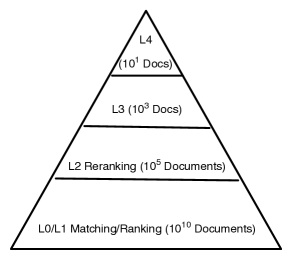
Figure 2: A four stage retrieval process as originally described by Pederson [30].

It is important to emphasize that the size of the candidate pool of documents $k$ is completely independent of the size of the final ranked list (with only the hard constraint that the final size has to be at least $k$). So, what is the proper setting of $k$? The work of Macdonald et al. [26] suggest several potential answers — “tens of thousands” (Chappelle and Chang [12]), $5{,}000$ (Craswell et al. [15]), $1{,}000$ (Qin et al. [31], or smaller samples such as $200$ (Zhang et al. [39]) or even $20$ (Cambazoglu et al. [9]). Of course, the larger the $k$, the slower the system, in two respects: First, in standard document-at-a-time query evaluation algorithms that would provide the initial candidate documents (e.g., Wand), $k$ has a direct impact on query latency, since a larger heap needs to be maintained, providing fewer opportunities for early exits depending on document score distributions. Second, for every document in the candidate pool, we need to run the feature extractors to serve as input to the subsequent reranking stages (see Figure 1). Thus, from an efficiency perspective, it is clear that we desire the smallest possible $k$ that allows end-to-end effectiveness to remain within some bounded envelope (see below for more details).

Note that our work focuses on the size of the candidate pool for the purposes of ranking at query time. In contrast, Macdonald et al. [26] focused on the importance of candidate pool size for the training of learning-to-rank systems. In particular, they looked at how the size of the candidate set effects the final results, arguing that the relationship is dependent on the type of information need. They show that as few as $10$-$20$ documents may be needed for TREC 2009 and 2010 web track queries, but as many as $1{,}500$ may be needed for navigational information needs on the same corpus. They also argue that field features such as anchor text are critical in the first stage retrieval process. Since we are concerned with the application of machine-learned models at runtime, the work of Macdonald et al. [26] is somewhat orthogonal to our study.

In terms of candidate generation, being able to control $k$ can have a substantial impact on end-to-end efficiency. An alternative approach might be, for a fixed $k$, to take advantage of approximate query evaluation algorithms that trade off the quality of the retrieved results for efficiency. As an example, Asadi and Lin [3] devised posting list intersection algorithms that take advantage of Bloom filters to generate result sets very quickly, but suffer from false positives, i.e., a retrieved document may not actually have all the query terms.

In this work, we explore a recently-developed and publicly available score-at-a-time approximate query evaluation algorithm proposed by Lin and Trotman [22] referred to as JASS. Instead of computing floating point document scores, their technique used quantized impact scores [1], which increases query evaluation speed by replacing floating point operations with simple integer additions to accumulate document scores while traversing postings. The query evaluation algorithm takes advantage of impact-ordered indexes to process posting segments in decreasing score order. Since contributions to the document scores monotonically decrease, query evaluation can quit at any time. Early termination is controlled by a parameter called $\rho$, which is simply the number of postings to be processed. As $\rho$ increases, the ranked list approaches that of exhaustive evaluation, which produces a precise ranking based on document scores.

Lin and Trotman [22] show that $\rho$ correlates linearly with wall-clock query evaluation time, with an $R^{2}$ value of over $0.9$ on Clue-Web09 and ClueWeb12 data. They further suggest that a $\rho$ setting equal to $10\%$ of the size of the collection achieves the best compromise between effectiveness and efficiency. Indeed, in a recent large-scale evaluation of open-source search engines [2], this new score-at-a-time approach was shown to be the fastest among all submissions. The suggested setting of $\rho$, however, was not fully explored, and furthermore is currently a global setting used for all queries.

It is clear that for candidate generation in multi-stage ranking, $k$ in Wand and $\rho$ in JASS represent important efficiency “knobs”. We would like to set both values as low as possible, but not sacrifice end-to-end effectiveness. This is, in short, the story and goal of this paper. We show that it is possible to predict, on a per-query basis, a minimum $k$ and $\rho$ such that end-to-end effectiveness remains within a bounded envelope, purely based on pre-retrieval static features, without requiring any relevance judgments.

The closest related work to ours is that of Tonellotto et al. [36], who also attempt to tune effectiveness-efficiency tradeoffs on a per query basis using query difficulty and query efficiency prediction techniques. However, their choice of settings is rather coarse grained: they only select between two configurations, whereas our classifier cascades are able to consider many more settings. Furthermore, their work exhibits the same limitation as most previous studies in requiring relevance judgments for training, and hence they are only able to experiment on 150 queries from TREC 2009–2011. In contrast, since our approach does not require any relevance judgments, we can tune our techniques on tens of thousands of queries, as we will discuss next.

2.2 Multi-Stage Ranking Effectiveness

Figure 3: Correlation between ${{\small\sf{MED}}_{\small{\small\sf{RBP}}}}$ and measured average precision using the 50 queries of the TREC 2010 Web Track adhoc collection and the IvoryL2Rb experimental run as the second-stage. Each of the $279$ points represents one of $31$ distinct first stages, across a range of parameter settings. The dashed line indicates the performance of the second stage with no early-stage filter. Reproduced from Tan and Clarke [35].

Tuning ranking parameters requires substantial training data to measure effectiveness. Fortunately, in the case of tuning candidate generation for a second-stage ranker (see Figure 1), we have this training data readily available, since the second stage itself may be enlisted to provide it. To create this training data we first run the second stage ranker over a very large candidate set, much larger than time might allow for interactive search. Conceptually this candidate set might be the entire collection, but practically it will be limited to a subset retrieved from query keyword matches and other simple features. Ideally, this set would contain all relevant documents, but mixed together with many non-relevant documents.

The second-stage ranker then ranks this set, producing a ranked list $A$. Given the potential size of the set, producing this ranking may take substantial time. However, while this time may be far greater than would be tolerable for interactive searching, when creating training data, time is not a problem.

Now, suppose we have a more efficient candidate generation algorithm, designed to feed this second stage ranker. It produces a much smaller set, which can be more efficiently ranked by the second stage to produce a ranked list $B$. We measure the effectiveness of the candidate generation algorithm according to its ability to supply the documents that the second stage needs in the absence of efficiency constraints, i.e., $A$. More specifically, we compute a rank correlation coefficient or rank similarity measure between $A$ and $B$, using its value $S(A,B)$ as our effectiveness metric.

Naturally, the similarity measure must be suitable for this purpose [37]. In particular, a rank similarity measure for search results must be appropriately top-weighed, placing greater emphasis on earlier ranks than on later ranks. If the top document in $A$ is missing from $B$, the impact on the user will be much greater than if the $100$th document is missing.

Tan and Clarke [35] describe a family of rank similarity measures specifically intended for comparing ranked lists produced by search engines. Given a traditional effectiveness metric — such as MAP [32], RBP [28], DCG [19], or ERR [11] —  Tan and Clarke define a distance measure between two ranked lists in terms of that metric, as follows: “Given two ranked lists, $A$ and $B$, what is the maximum difference in their effectiveness scores possible under [that metric].”

They call this family of distance measures maximized effectiveness difference (MED$(A,B)$) and develop variants corresponding to several standard effectiveness metrics — including ${{\small\sf{MED}}_{\small{\small\sf{MAP}}}}$, ${{\small\sf{MED}}_{\small{\small\sf{RBP}}}}$, ${{\small\sf{MED}}_{\small{\small\sf{DCG}}}}$, and ${{\small\sf{MED}}_{\small{\small\sf{ERR}}}}$. They explore MED as a method for quantifying changes to ranking algorithms without the need for human relevance judgments. For example, MED allows a search to identify queries for which a proposed change causes the greatest impact. An open-source implementation is publicly available online, which can be used to compute MED for various effectiveness measures, and is used in this paper.

Building on this work, we have recently applied MED to measure effectiveness of the initial stages in multi-stage rankers [14]. That work follows the procedure outlined above, using a second-stage ranking as a gold standard to measure first-stage effectiveness, validating this procedure. Unlike previous explorations of efficiency-effectiveness tradeoffs, the absence of any requirement for human relevance judgments allows the procedure to be easily applied across tens of thousands of queries.

For illustration purposes, Figure 3 is reproduced from that paper. The figure shows the performance of a number of first-stage rankers, operating over a range of parameter settings, supplying a high-quality second-stage ranker. The horizonal dashed line indicates the performance of the second-stage ranker without first-stage filtering. Values of ${{\small\sf{MED}}_{\small{\small\sf{RBP}}}}$ below 0.05 produce no practical loss in measured effectiveness.

In this range, MED is measuring shortcomings in the first-stage that are not necessarily reflected in the evaluation measures. A first-stage ranker that fails to return the top document required by the second stage will receive a lower MED score than a first-stage ranker that fails to return the sixth document. While other relevant documents might move up to replace the lost documents, leaving both with the same measured effectiveness, losing the top-ranked document is viewed more seriously than losing lower-ranked documents.

Previous work explored efficiency-effectiveness tradeoffs of first-stage algorithms, and their parameter settings, as applied uniformly across all queries (including the blinded citation above). However, optimal algorithms and settings vary across queries. In this paper we explore a technique for optimizing efficiency-effectiveness tradeoffs on a per-query basis, selecting the optimal algorithm and setting for each using static, pre-retrieval features. While we focus specifically on the two-stage architecture in Figure 1, our methods should generalize to larger multistage architectures, such as shown in Figure 2, with the effectiveness of each stage measured in terms of the next.

3 Approach

Feature Selection.  Simple term features have been used successfully in a variety of different learning to rank scenarios  [23, 24, 26, 27] and in query difficulty prediction [10, 25, 20]. Across all of this work one general theme has emerged – a mixture of similarity measures and query specific score aggregation techniques yield the most benefit. Inspired by this previous work, we adopt this philosophy in our feature choices as well. We use three simple similarity measures in this work:

1. BM25 with the formulation:

   $$\hphantom{1}{\mbox{\scriptsize BM25}}=\log\left(\frac{N-f_{t}+0.5}{f_{t}+0.5}\right)\cdot{\mbox{TF}_{\mbox{\scriptsize{BM25}}}}$$

   $${\mbox{TF}_{\mbox{\scriptsize{BM25}}}}=\frac{f_{t,d}\cdot(k_{1}+1)}{f_{t,d}+k_{1}\cdot((1-b)+(b\cdot\ell_{d}/\ell_{avg}))}$$

   where $N$ is the number of documents in the collection, $f_{t}$ is the number of distinct document appearances of $t$, $f_{d,t}$ is the number of occurrences of term $t$ in document $d$, $k_{1}=0.9$, $b=0.4$ , $\ell_{d}$ is the number of terms in document $d$, and $\ell_{avg}$ is the average of $\ell_{d}$ over the whole collection.

2. Query Likelihood using a Dirichlet prior smoothing formulation:

   $$\hphantom{1}{\mbox{\scriptsize LM}}=\log\left(\frac{f_{t,d}+\mu\cdot C_{t}/|C|}{\ell_{d}+\mu}\right)$$

   where $C_{t}$ is the number of occurrences of $t$ in the collection, $|C|$ is the length of the collection (total number of terms), $\mu=2500$ is the smoothing factor, and all other variables are the same as in BM25.

3. tf$\times$idf with the formulation:

   $$\hphantom{1}{\mbox{{tf}$\times${idf}}}=\frac{1}{\ell_{d}}\cdot(1+\log(f_{t,d}))\cdot\log(1+\frac{N}{f_{t}})$$

Term Statistics
1. Number of occurrences of term $t$ in collection ($C_{t}$).
2. Number of documents containing term $t$ ($f_{t}$).
3. Maximum Similarity Score
4. First Quartile Similarity Score
5. Third Quartile Similarity Score
6. Minimum Similarity Score
7. Arithmetic Mean of Similarity Scores
8. Harmonic Mean of Similarity Scores
9. Median of Similarity Scores
10. Variance of Similarity Scores
11. Interquartile Range of Similarity Scores

Table 1: Query independent term features used by the classifier. Each feature can be precomputed and stored with the postings list.

Query Features (Score Dependent)

1. Arithmetic Mean of $t_{f}$

2. Harmonic Mean of Maximum Scores

3. Arithmetic Mean of Maximum Scores

4. Arithmetic Mean of Median Score

5. Arithmetic Mean of Mean Scores

6. Arithmetic Mean of Score Variances

7. Arithmetic Mean of Score Interquartile Ranges

8. Minimum Score of terms in the query for each feature in Table 1.

9. Maximum Score of terms in the query for each feature in Table 1.

Query Features (Score Independent)

1. Query Length

Table 2: Query specific features used by the classifier. All score dependent features can be computed on the fly for all three similarity metrics at query time using the prestored values in Table 1.

Topic	$k$
	$20$	$50$	$100$	$200$	$500$	$1{,}000$	$2{,}000$	$5{,}000$	$10{,}000$
20001	0.544	0.346	0.104	0.056	0.010	0.002	0.001	0.000	0.000
20002	0.536	0.142	0.053	0.016	0.002	0.000	0.000	0.000	0.000
20003	0.865	0.856	0.810	0.773	0.706	0.684	0.582	0.122	0.000
20004	0.999	0.944	0.132	0.070	0.018	0.008	0.008	0.000	0.000

Table 3: The ${{{\small\sf{MED}}_{\small{\small\sf{RBP}}}}}$ scores for the first four topics in the TREC MQ2009 collection at $9$ different cutoffs for $k$.

These similarity formulations were used since each can easily be precomputed for all term—document combinations and treated as independent term-specific features. In addition to the three similarity scoring regimes, we also adopt several different score aggregation techniques, and compute a variety of static statistical features for each term posting: maximum score, minimum score, arithmetic mean of scores, harmonic mean of scores, median of scores, variance of scores, first quartile score, and third quartile score. Additional query specific features are also incorporated into the model including query length, minimum and maximum score for the terms in the query, and means (arithmetic and harmonic) of the query specific term scores. Table 1 provides a comprehensive breakdown of the term specific features, each of which can be computed at index time. Table 2 shows how each of the term specific features are combined into the final feature set used by the classifier. A total of $70$ features are used in our work.

Labeling Instances.  We now turn our attention to how the training collection was created. One of the key ideas of this work is to use MED to determine a minimal candidate set that also maximizes the possible effectiveness in the final reranking stage. In order to achieve this, we have created a gold standard set using $40{,}000$ queries from the 2009 TREC Million Query Track. For each query, ${{\small\sf{MED}}_{\small{\small\sf{RBP}}}}$, ${{\small\sf{MED}}_{\small{\small\sf{ERR}}}}$, and ${{\small\sf{MED}}_{\small{\small\sf{DCG}}}}$ is computed for the $k$ values of $20$, $50$, $100$, $200$, $500$, $1{,}000$, $2{,}000$, $5{,}000$, and $10{,}000$. Our gold standard run for tuning $k$ was the uogTRMQdph40 run, as it represents one of the top-scoring systems (when measured over the small subset of the queries that were evaluated) that returned results for all $40{,}000$ of the MQ2009 queries. For $\rho$, the cutoff values were $100$k, $200$k, $500$k, $1$m, $2$m, $5$m, $10$m, $20$m, and $50$m. Our gold standard run for tuning $\rho$ is the ranked list that results from exhaustive query evaluation, which generates an exact ranking.

So, in total we have computed MED using three different metrics at $9$ distinct cutoffs for $k$ and $\rho$. To label the instances, we now select a sufficiently low value of a given metric, say ${{\small\sf{MED}}_{\small{\small\sf{RBP}}}}\leq 0.05$, and choose the minimal cutoff that satisfies this constraint—this is what we have previously referred to as the “effectiveness envelope” we would like to maintain.

For example, consider the ${{\small\sf{MED}}_{\small{\small\sf{RBP}}}}$ computations for the first $4$ topics shown in Table 3. If the minimal acceptable score is ${{\small\sf{MED}}_{\small{\small\sf{RBP}}}}\leq 0.05$, then for Topic $20001$, the nominal class assigned would be $k=500$, whereas Topic $20002$ can achieve a similar score with $k=200$.

$$\mathcal{C}=\begin{pmatrix}\kern 4.0pt0&1&1&1&1&1&1&1&1\kern 4.0pt\\ \kern 4.0pt2&0&1&1&1&1&1&1&1\kern 4.0pt\\ \kern 4.0pt3&2&0&1&1&1&1&1&1\kern 4.0pt\\ \kern 4.0pt4&3&2&0&1&1&1&1&1\kern 4.0pt\\ \kern 4.0pt5&4&3&2&0&1&1&1&1\kern 4.0pt\\ \kern 4.0pt6&5&4&3&2&0&1&1&1\kern 4.0pt\\ \kern 4.0pt7&6&5&4&3&2&0&1&1\kern 4.0pt\\ \kern 4.0pt8&7&6&5&4&3&2&0&1\kern 4.0pt\\ \kern 4.0pt9&8&7&6&5&4&3&2&0\kern 4.0pt\\ \end{pmatrix}$$

Figure 4: A nine class cost matrix which penalizes underpredictions in a classifier.

Multilabel Classification and Regression.  The most obvious solution from a machine learning perspective is to train a multilabel classifier, or use the true cutoff values with a regression algorithm such as a Reduced Error Pruning Tree (REPTree) [18], a Multilayer Perceptron, or Sequential Minimal Optimization (SMOReg) [34]. We explored all of these possibilities in our early empirical analysis, and found that none of the approaches was reliably better than using a fixed cutoff baseline.

After careful examination of the initial results, a clear constraint emerged in producing good results in our classifier — any under-prediction (False Positives) can significantly hurt overall effectiveness and should be avoided. A standard approach to reweight classification is to use a cost sensitive classifier [17] such as MetaCost [16]. Our experiments with a cost sensitive classifier that penalized the classifier for under-predicting (false positives) were promising. For example, using the cost matrix $\mathcal{C}$ shown in Figure 4 provides a better solution than either a multilabel classification or a regression. At the bottom of the matrix, we penalize instances that have the highest label very heavily for under-predictions. Conversely, we do not penalize the meta-classifier for over predicting.

There has also been recent work on building cost sensitive regression algorithms [40], but this is still an active area of research and beyond the scope of our work. Instead, we embrace and extend another common technique in regression — choosing a fixed threshold and creating a binary classifier. However, we found that a single threshold was not sufficient for our needs, and that the approach could be extended to make a series of binary predictions to find the best cutoffs. We explain the mechanics of this technique next.

Cascaded Classification.  Our approach to prediction relies on a cascade of binary classifiers. Since classes are ordinal and should be treated as such, a series of binary predictions can be used to find the minimum cutoff for each query that also maximizes the overall effectiveness in the final document reordering stage. Our approach is similar in spirit to the cascade of classifiers developed by Chen et al. [13], and later extended by Xu et al. [38] to minimize the costs of feature evaluation.

Algorithm 1 MultiClassToBinary

1:A set of queries $Q$, and an optimal cutoff selected from $c$ choices.

2:A total of $c-1$ binary training sets $\mathcal{B}$

3:for $i=1$ to $c-1$ do

4:     for $q=0$ to $|Q|$ do

5:         if Class($q)\leq c$ then

6:              Class ($\mathcal{B}_{i}$[$q$]) $\leftarrow 0$

7:         else

8:              Class($\mathcal{B}_{i}$[$q$]) $\leftarrow 1$

9:         end if

10:     end for

11:end for

12:Return $\mathcal{B}$

In this work, a random forest classifier [6] is trained and used for predictions at each stage of the cascade. Before building the classifier, training sets can be created from a multilabeled class set. The number of binary classifiers required is $c-1$ where $c$ is the maximum ordinal label. Labels should be monotonically increasing from $1$ to $c$. Algorithm 1 shows the approach used to generate a training set that can be used for iterated binary classifications.

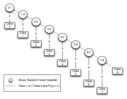
Figure 5: A left-to-right nine class cascade. Each node is a binary, random forest classifier. If the classifier predicts $0$ with a probability $\mbox{\emph{Pr}}(p)>t$, the current node ID is written as the class. Otherwise, the instance is passed to the next classifier in the chain.

Algorithm 2 LRCascade

1:A query $q$, a minimum confidence threshold $t$, and a set of $c-1$ binary classifiers $\mathcal{C}$

2:A cutoff prediction between $1$ and $c$.

3:for $i=1$ to $c-1$ do

4:     $p\leftarrow$ Predict($C_{i}$,$q$)

5:     if $p=0$ and $Pr(p)>t$ then

6:         Return $i$

7:     end if

8:end for

9:Return $c$

Once the binary classifiers are constructed, it is relatively simple to make a prediction for any query $q$. A feature set can easily be constructed at query parsing time which is then used by Algorithm 2 to assign a cutoff for the query. A left-to-right cascade serves two important purposes. First, the model implicitly minimizes the likelihood of a false positive as assignments are made smallest to largest, and exits only occur for high probability predictions. Secondly, each prediction has a small cost. In a left-to-right cascade, queries with the smallest cutoff incur the least amount of processing time. If a larger cutoff is required, the cost of extra predictions is small relative to the cost of more expensive reordering stages of large candidate sets later in the scoring process.

Figure 5 shows an example of a left-to-right nine class cascade of binary classifiers. Each node in the tree is a binary random forest classifier pre-trained using one of $\mathcal{B}$ training sets generated using Algorithm 1. By increasing the cutoff threshold $t$, the percentage of under-predictions is decreased at the cost of increasing the percentage of over-predictions. However, some level of over-prediction is always acceptable as this always results in a gradual increase in overall effectiveness.

4 Experiments

Experimental Configuration.  For all experiments, $40{,}000$ queries from the 2009 Million Query Track (MQ2009) were used with a stopped and unpruned ClueWeb 2009 category B index (CW09B). The uogTRMQdph40 system is used as the gold standard, as it represents one of the top-scoring systems (when measured over the small subset of the queries that were evaluated) that returned runs for all $40{,}000$ MQ2009 queries. Specifically, this is the highest scoring system that submitted results for all of the queries in MQ2009, making it the best choice as the gold standard in our work.

To generate the bag-of-words candidate run, a BM25 implementation using the same formulation and parameterization as described in Section 3 was ran for all $40{,}000$ MQ2009 queries. The stopword list and Krovetz stemmer were derived directly from the Indri search engine. A total of $50{,}22{,}0423$ documents were indexed from the CW09B collection, and all queries were ran to a depth of $10{,}000$.

For classification, the $k$ and $\rho$ values were computed at nine different positions. For $k$, the values were $20$, $50$, $100$, $200$, $500$, $1{,}000$, $2{,}000$, $5{,}000$, and $10{,}000$. For $\rho$, the values were $100$k, $200$k, $500$k, $1$m, $2$m, $5$m, $10$m, $20$m, and $50$m. For each bucket, three different MED variants were computed: ${{\small\sf{MED}}_{\small{\small\sf{RBP}}}}$, ${{\small\sf{MED}}_{\small{\small\sf{ERR}}}}$, and ${{\small\sf{MED}}_{\small{\small\sf{DCG}}}}$. Cross validation was performed by partitioning all of the queries into $10$ folds using the StratifiedRemoveFolds filter in Weka-3.7.13. Then, $10$ runs of each classification approach were ran using $9$ folds for training, and the current fold for testing to generate a prediction for each topic in the collection. Note that before generating the final folds, we removed all queries for which we had any judgments ($687$ topics) at all, for further validation purposes.

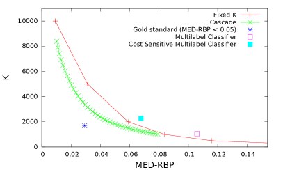
Figure 6: ${{\small\sf{MED}}_{\small{\small\sf{RBP}}}}$ versus $k$ when using a training threshold cutoff of ${{\small\sf{MED}}_{\small{\small\sf{RBP}}}}\leq 0.05$ (left panel) and ${{\small\sf{MED}}_{\small{\small\sf{RBP}}}}\leq 0.10$ (right panel) for the MQ2009 queries on ClueWeb09B. The blue star represents the best possible result achievable with a “perfect” classifier, the green line is the result when using our LR Binary Cascade Model, and the red line represents the tradeoff horizon based on using a fixed $k$ for all queries.

Dynamic Selection of $k$.  Our first set of experiments were designed to test the hypothesis that a best $k$ value can be determined on a query by query basis which minimizes effectiveness loss, and maximizes efficiency. In other words, finding the smallest acceptable $k$ for a targeted MED value can minimize the amount of work later stage rerankers must do, and also minimizes the cost of using a safe-to-$k$ candidate generation algorithm such as Wand. In order to prove this hypothesis, we created several different datasets to train our predictor. We experimented with ${{\small\sf{MED}}_{\small{\small\sf{RBP}}}}$ using the cutoffs $0.02$, $0.05$, $0.10$, $0.15$, $0.20$, $0.25$, $0.30$, and $0.50$. We also experimented with ${{\small\sf{MED}}_{\small{\small\sf{DCG}}}}$ using the cutoffs $0.2$, $0.3$, $0.5$, $0.7$, $1.00$, $1.20$, and $1.50$. Similar experiments were performed with ${{\small\sf{MED}}_{\small{\small\sf{ERR}}}}$ using the cutoffs $0.05$, $0.10$, $0.15$, $0.20$, $0.25$, $0.30$, and $0.50$.

Figure 6 shows the tradeoff achievable between the candidate set size $k$ and ${{\small\sf{MED}}_{\small{\small\sf{RBP}}}}$. The left pane is a summary of results when using a target of ${{\small\sf{MED}}_{\small{\small\sf{RBP}}}}\leq 0.05$, and the right pane summarizes method performance for ${{\small\sf{MED}}_{\small{\small\sf{RBP}}}}\leq 0.10$. In both graphs, the red line represents the tradeoff horizon in efficiency and effectiveness when using a fixed cutoff for all queries as is generally done in current system configurations. The blue star represents the gold standard result that would be achievable with a “perfect” classifier. The two squares represent the result achievable when using standard machine learning approaches such as a Bayesian Model Combination, boosted, multilabel random forest classifier [29] , or a Cost Sensitive Classifier such as MetaCost [16] . When compared to the fixed baseline, we see that a traditional approach to classification does not provide any real benefit.

In contrast, the LRCascade approach (green line) shows clear improvements over both multi-label and fixed cutoff approaches. The lower the choice of MED, the less likely there is any loss in effectiveness. Our experiments suggest that targeting low MED values are likely to reap the most rewards. This is, the process of minimizing effectiveness loss greatly benefits from a variable cutoff approach.

Method		Interpolated ${{{\small\sf{MED}}_{\small{\small\sf{RBP}}}}}$					Interpolated $k$
		Predicted	Predicted	Fixed	Difference in		Predicted	Predicted	Fixed	Difference in
		${{{\small\sf{MED}}_{\small{\small\sf{RBP}}}}}$	$k$	$k$	$k$		$k$	${{{\small\sf{MED}}_{\small{\small\sf{RBP}}}}}$	${{{\small\sf{MED}}_{\small{\small\sf{RBP}}}}}$	${{{\small\sf{MED}}_{\small{\small\sf{RBP}}}}}$
Oracle		$0.029$	$1{,}688$	$5{,}459$	+$223\%$		$1{,}688$	$0.029$	$0.067$	+$128\%$
MultiLabel		$0.106$	$1{,}053$	$\hphantom{1,}653$	–$\hphantom{1}38\%$		$1{,}053$	$0.106$	$0.082$	–$\hphantom{1}22\%$
MetaCost		$0.068$	$2{,}277$	$1{,}644$	–$\hphantom{1}28\%$		$2{,}277$	$0.068$	$0.056$	–$\hphantom{1}16\%$
LRCascade, $t=0.75$		$0.045$	$2{,}071$	$3{,}535$	+$\hphantom{1}71\%$		$2{,}071$	$0.045$	$0.058$	+$\hphantom{1}30\%$
LRCascade, $t=0.80$		$0.036$	$2{,}656$	$4{,}432$	+$\hphantom{1}67\%$		$2{,}656$	$0.036$	$0.053$	+$\hphantom{1}45\%$
LRCascade, $t=0.85$		$0.028$	$3{,}561$	$5{,}715$	+$\hphantom{1}61\%$		$3{,}561$	$0.028$	$0.044$	+$\hphantom{1}59\%$

Table 4: Interpolated $k$ and ${{{\small\sf{MED}}_{\small{\small\sf{RBP}}}}}$ when training at ${{{\small\sf{MED}}_{\small{\small\sf{RBP}}}}}\leq 0.05$. The relative gain or loss for $k$ and ${{{\small\sf{MED}}_{\small{\small\sf{RBP}}}}}$ are shown when compared to using a fixed cutoff for all queries. The Oracle method represents the best possible result given a perfect classifier.

Table 4 shows the breakdown for using a fixed $k$ and predicted $k$ interpolation when using a training set targeted at ${{\small\sf{MED}}_{\small{\small\sf{RBP}}}}\leq 0.05$. Columns $2$–$5$ show the relative gain in terms of $k$, and columns $6$–$9$ show the relative gain in terms of ${{\small\sf{MED}}_{\small{\small\sf{RBP}}}}$. The first row shows the gold standard Oracle result, which represents the best result that is achievable using this parameter – metric – target threshold combination. Changing any one of these three constraints will change the gain (or loss) possible. In other words, just computing the Oracle result is in itself interesting, as it provides a bound on how much benefit the three constraint combination could provide.

The interpretation of the data in columns $2$–$5$ is as follows: given a particular setting, how far below the interpolated fixed $k$ curve (red) are we? That is, if we accept a particular level of ${{\small\sf{MED}}_{\small{\small\sf{RBP}}}}$ effectiveness, how much efficiency can we gain over simply just adopting a fixed $k$ cutoff for all queries (specifically, the $k$ cutoff that would achieve the same level of ${{\small\sf{MED}}_{\small{\small\sf{RBP}}}}$)? The interpretation of the data in columns $6$–$9$ is as follows: given a particular setting, how far left of the interpolated fixed $k$ curve (red) are we? That is, how much more effective (in terms of ${{\small\sf{MED}}_{\small{\small\sf{RBP}}}}$) can we make our results over simply setting a fixed $k$? In designing actual search architectures, the first interpretation is more intuitive, since we want to optimize efficiency without sacrificing effectiveness, but the alternative perspective is interesting as well in quantifying the benefits of our technique.

We see that both MultiLabel and MetaCost are marginally worse than a fixed cutoff, with MetaCost being the slightly better choice. The LRCascade method is the clear winner across a wide range of $t$. The exact value of $t$ can be set depending on which direction a user wishes to bias the tradeoff. Choosing a lower $t$ decreases the average $k$, while increasing the average ${{\small\sf{MED}}_{\small{\small\sf{RBP}}}}$. Choosing a higher $t$ biases the tradeoff in the effectiveness direction.

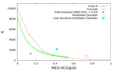
Figure 7: ${{\small\sf{MED}}_{\small{\small\sf{DCG}}}}$ versus $k$ when using a training threshold cutoff of ${{\small\sf{MED}}_{\small{\small\sf{DCG}}}}\leq 0.50$ (left panel) and ${{\small\sf{MED}}_{\small{\small\sf{DCG}}}}\leq 1.0$ (right panel) for the MQ2009 queries on ClueWeb09B. The blue star represents the best possible result achievable with a “perfect” classifier, the green line is the result when using our LR Binary Cascade Model, and the red line represents the tradeoff horizon based on using a fixed $k$ for all queries.

Figure 7 shows the same experiment when using ${{\small\sf{MED}}_{\small{\small\sf{DCG}}}}\leq 0.50$ and ${{\small\sf{MED}}_{\small{\small\sf{DCG}}}}\leq 1.00$. Changing the underlying evaluation metric does not change the general trends for all methods tested. Multilabel classifiers do not outperform fixed cutoffs, while the LRCascade is the superior tradeoff. We also ran a similar set of experiments using ${{\small\sf{MED}}_{\small{\small\sf{ERR}}}}$ and achieved similar results and trends.

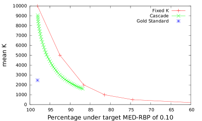
Figure 8: Average $k$ versus the percentage of queries achieving a MED score less than a training target. The left panel shows the comparison of the LRCascade (green line) and a fixed cutoff (red line) for ${{\small\sf{MED}}_{\small{\small\sf{RBP}}}}\leq 0.10$. The right panel shows the same comparison when using ${{\small\sf{MED}}_{\small{\small\sf{DCG}}}}\leq 0.50$.

Figure 8 shows the percentage of queries which obtain a bound of ${{\small\sf{MED}}_{\small{\small\sf{RBP}}}}\leq 0.10$ or ${{\small\sf{MED}}_{\small{\small\sf{DCG}}}}\leq 0.50$. We can see that the LRCascade approach is clearly predicting cutoffs which have a lower mean $k$, and a higher percentage of queries under the target MED, translating into better effectiveness. You may notice that even the gold standard does not achieve 100% under ${{\small\sf{MED}}_{\small{\small\sf{RBP}}}}$. For a proportion of the topics our first stage returns less than the target $K$ documents due to a lack of documents containing any of the query terms. Since ${{\small\sf{MED}}_{\small{\small\sf{RBP}}}}$, like RBP, is conceptually evaluated to infinite depth, this deficiency is reflected by positive scores, some of which fall above the targeted value. On the other hand, ${{\small\sf{MED}}_{\small{\small\sf{DCG}}}}$ is evaluated to fixed depth (depth 20 in this case) and the gold standard achieves 100%.

Method		Interpolated ${{{\small\sf{MED}}_{\small{\small\sf{ERR}}}}}$					Interpolated $k$
		Predicted	Predicted	Fixed	Difference in		Predicted	Predicted	Fixed	Difference in
		${{{\small\sf{MED}}_{\small{\small\sf{ERR}}}}}$	$k$	$k$	$k$		$k$	${{{\small\sf{MED}}_{\small{\small\sf{ERR}}}}}$	${{{\small\sf{MED}}_{\small{\small\sf{ERR}}}}}$	${{{\small\sf{MED}}_{\small{\small\sf{ERR}}}}}$
Oracle		$0.017$	$1{,}752$	$7{,}344$	+$319\%$		$1{,}752$	$0.017$	$0.067$	+$292\%$
MultiLabel		$0.117$	$1{,}159$	$\hphantom{1,}452$	–$\hphantom{1}61\%$		$1{,}159$	$0.117$	$0.082$	–$\hphantom{1}30\%$
MetaCost		$0.060$	$3{,}222$	$2{,}214$	–$\hphantom{1}31\%$		$3{,}222$	$0.060$	$0.050$	–$\hphantom{1}16\%$
LRCascade, $t=0.75$		$0.047$	$2{,}206$	$3{,}465$	+$\hphantom{1}57\%$		$2{,}206$	$0.047$	$0.060$	+$\hphantom{1}26\%$
LRCascade, $t=0.80$		$0.035$	$3{,}013$	$4{,}705$	+$\hphantom{1}56\%$		$3{,}013$	$0.035$	$0.052$	+$\hphantom{1}47\%$
LRCascade, $t=0.85$		$0.024$	$4{,}191$	$6{,}351$	+$\hphantom{1}52\%$		$4{,}191$	$0.024$	$0.040$	+$\hphantom{1}70\%$

Table 5: Interpolated $k$ and ${{{\small\sf{MED}}_{\small{\small\sf{ERR}}}}}$ when training at ${{{\small\sf{MED}}_{\small{\small\sf{ERR}}}}}\leq 0.05$. The relative gain or loss for $k$ and ${{{\small\sf{MED}}_{\small{\small\sf{ERR}}}}}$ are shown when compared to using a fixed cutoff for all queries. The Oracle method represents the best possible result given a perfect classifier.

Finally, Table 5 shows the breakdown for several fixed $k$ and predicted $k$ interpolations when building the training set to target ${{\small\sf{MED}}_{\small{\small\sf{ERR}}}}\leq 0.05$. The trends remain consistent as when using ${{\small\sf{MED}}_{\small{\small\sf{RBP}}}}$ or ${{\small\sf{MED}}_{\small{\small\sf{DCG}}}}$. The most interesting aspect of this table is to note the subtle difference in potential improvements possible for the gold standard Oracle result. Potential gains are +$319\%$ and +$292$ respectively. This is a little better than the Oracle result for ${{\small\sf{MED}}_{\small{\small\sf{RBP}}}}$ shown in Table 4, or that of ${{\small\sf{MED}}_{\small{\small\sf{DCG}}}}\leq 0.50$ which shows potential gains of +$259\%$ for $k$ and +$147$ for MED. Potential gains are sensitive to both training cutoff and metric, which should come as no surprise to the reader.

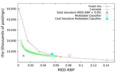
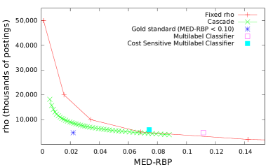
Figure 9: ${{\small\sf{MED}}_{\small{\small\sf{RBP}}}}$ versus $\rho$ when using a training threshold cutoff of ${{\small\sf{MED}}_{\small{\small\sf{RBP}}}}\leq 0.05$ (left panel) and ${{\small\sf{MED}}_{\small{\small\sf{RBP}}}}\leq 0.10$ (right panel) for the MQ2009 queries on ClueWeb09B. The blue star represents the best possible result achievable with a “perfect” classifier, the green line is the result when using our LR Binary Cascade Model, and the red line represents the tradeoff horizon based on using a fixed $k$ for all queries.

Dynamic Selection of $\rho$.  We now turn our attention to the parameter $\rho$. The $\rho$ parameter controls the number of postings scored using a score-at-a-time approximation algorithm. Quite simply, it is a parameter that can be used to tune an efficiency-effectiveness tradeoff. Our methodology is identical to the approach taken for $k$. The only difference is the initial generation of the cutoff data that is used for training the classifier.

Figure 9 shows the effect of ${{\small\sf{MED}}_{\small{\small\sf{RBP}}}}$ for the training cutoffs $0.05$ and $0.10$. When comparing both graphs we can see that training with a smaller cutoff provides a clear advantage. The gold standard point provides an ambitious goal. Once again the LRCascade approach is clearly better than the fixed cutoff in both dimensions, MED and $\rho$.

Method		Interpolated ${{{\small\sf{MED}}_{\small{\small\sf{RBP}}}}}$					Interpolated $\rho$
		Predicted	Predicted	Fixed	Difference in		Predicted	Predicted	Fixed	Difference in
		${{{\small\sf{MED}}_{\small{\small\sf{RBP}}}}}$	$\rho$	$\rho$	$\rho$		$\rho$	${{{\small\sf{MED}}_{\small{\small\sf{RBP}}}}}$	${{{\small\sf{MED}}_{\small{\small\sf{RBP}}}}}$	${{{\small\sf{MED}}_{\small{\small\sf{RBP}}}}}$
Oracle		$0.009$	$\hphantom{1}6{,}094$	$34{,}085$	+$459\%$		$\hphantom{1}6{,}094$	$0.009$	$0.061$	+$575\%$
MultiLabel		$0.082$	$\hphantom{1}6{,}656$	$\hphantom{1}4{,}434$	–$\hphantom{1}33\%$		$\hphantom{1}6{,}656$	$0.082$	$0.057$	–$\hphantom{1}31\%$
MetaCost		$0.054$	$\hphantom{1}7{,}787$	$\hphantom{1}7{,}032$	–$\hphantom{1}10\%$		$\hphantom{1}7{,}787$	$0.054$	$0.049$	–$\hphantom{1}\hphantom{1}9\%$
LRCascade, $t=0.75$		$0.026$	$\hphantom{1}8{,}430$	$14{,}350$	+$\hphantom{1}70\%$		$\hphantom{1}8{,}430$	$0.026$	$0.045$	+$\hphantom{1}72\%$
LRCascade, $t=0.80$		$0.021$	$\hphantom{1}9{,}388$	$17{,}318$	+$\hphantom{1}84\%$		$\hphantom{1}9{,}388$	$0.021$	$0.038$	+$\hphantom{1}86\%$
LRCascade, $t=0.85$		$0.016$	$10{,}532$	$20{,}239$	+$\hphantom{1}92\%$		$10{,}532$	$0.016$	$0.033$	+$113\%$

Table 6: Interpolated $\rho$ and ${{{\small\sf{MED}}_{\small{\small\sf{RBP}}}}}$ when training at ${{{\small\sf{MED}}_{\small{\small\sf{RBP}}}}}\leq 0.05$. The relative gain or loss for $\rho$ and ${{{\small\sf{MED}}_{\small{\small\sf{RBP}}}}}$ are shown when compared to using a fixed cutoff for all queries. The Oracle method represents the best possible result given a perfect classifier. Note that $\rho$ values are in thousands of postings scored.

Table 6 shows the ${{\small\sf{MED}}_{\small{\small\sf{RBP}}}}$ and $\rho$ interpolation results when training the classifier with a cutoff of ${{\small\sf{MED}}_{\small{\small\sf{RBP}}}}\leq 0.05$. Again the results are consistent with the general trends observed in Table 4. One key difference is that the potential gain in the tradeoff achievable by the Oracle method relative to using a fixed cutoff is $2\times$ in terms of efficiency, and $4\times$ in effectiveness. This translates directly into higher relative gains achievable using our LRCascade approach.

There are several interesting insights that can be gleaned from this experiment. Firstly, our classification approach is generalizable. We use exactly the same feature sets, algorithms, and prediction methodology in both experiments. The only key difference is in the construction of the training data.

Perhaps further improvements could be realized by tuning a number of different configuration options such as the number of class cutoffs, using variable cutoff thresholds $t$ at different nodes in the cascade, changing the classifier algorithms (perhaps even using different classifiers) at different nodes in the cascade, or even developing an entirely new approach to cascaded regression / classification. Initial efforts towards variable cutoff thresholds show promising results. The gains achievable are independent to all of these decisions. In fact the precise gain can be computed based on the creation of the Oracle run before investing any time and effort into engineering a feature set and classification scheme.

Method	NDCG@10	ERR	k
Oracle	0.356	0.434	2,386
LRCascade, $t=0.75$	0.359	0.435	3,422
LRCascade, $t=0.80$	0.359	0.435	4,062
LRCascade, $t=0.85$	0.358	0.435	5,130
Fixed, $k=10,000$	0.358	0.434	10,000

Table 7: Measured performance over 50 held out TREC 2009 Web Track adhoc queries.

Validation  As a final step, we confirmed our past experience (as illustrated by Figure 3) that low ${{\small\sf{MED}}_{\small{\small\sf{RBP}}}}$ values produce minimal loss in measured effectiveness. For this purpose we employed the 50 queries of the TREC 2009 Web Track adhoc task, which were held out from the training and test sets of other experiments reported in this section. These 50 queries were pooled to depth 12 for judging, and so should at least be suitable for computing early-precision effectiveness measures, including NDCG@10 and ERR.

Table 7 shows the results. Over these queries, our cascade classifier produces no measurable loss in effectiveness when compared to a fixed $k$ of $10{,}000$. In fact, the classifer achieves a tiny (but not significant) gain in effectiveness in the third decimal place of some measures, reflecting a change of one or two documents across this small query set. On the other hand, there are substantial reductions in average $k$, reflecting expected efficiency improvements.

5 Conclusion

In this work, we have presented a new query specific approach to dynamically predict the best parameter cutoffs that maximises both efficiency and effectiveness. To achieve this, we use Maximized Effectiveness Difference (MED) [35, 14] as the basis for evaluating the quality of a candidate set relative to a more expensive gold standard reranking step. By extending this methodology, we are able to create a large test corpora, and train a remarkably robust classifier which requires no relevance judgements. Our approach to binary cascaded classification is able to achieve up to a $50\%$ improvement in average $k$. For $\rho$, we achieve up to an even greater relative improvement in average number of postings scored. Our approach can easily be generalized to effectively tune a wide variety of other parameters dynamically in multi-stage retrieval systems, and can be used to reliable estimate potential gains achievable with any parameter — metric — target threshold combination.

Acknowledgments.  This work was partially supported by the Natural Sciences and Engineering Research Council of Canada (NSERC), and by the Australian Research Council’s Discovery Projects Scheme (DP140103256). Shane Culpepper is the recipient of an Australian Research Council DECRA Research Fellowship (DE140100275).

References

- Anh et al. [2001] V. N. Anh, O. de Kretser, and A. Moffat. Vector-space ranking with effective early termination. In Proc. SIGIR, pages 35–42, 2001.
- Arguello et al. [2015] J. Arguello, M. Crane, F. Diaz, J. Lin, and A. Trotman. Report on the SIGIR 2015 Workshop on Reproducibility, Inexplicability, and Generalizability of Results (RIGOR). volume 49, pages 107–116, 2015.
- Asadi and Lin [2012] N. Asadi and J. Lin. Fast candidate generation for two-phase document ranking: Postings list intersection with Bloom filters. In Proc. CIKM, pages 2419–2422, 2012.
- Asadi and Lin [2013a] N. Asadi and J. Lin. Document vector representations for feature extraction in multi-stage document ranking. Inf. Retr., 16(6):747–768, 2013a.
- Asadi and Lin [2013b] N. Asadi and J. Lin. Effectiveness/efficiency tradeoffs for candidate generation in multi-stage retrieval architectures. In Proc. SIGIR, pages 997–1000, 2013b.
- Breiman [2001] L. Breiman. Random forests. Machine Learning, 45(1):5–32, 2001.
- Burges [2010] C. Burges. From ranknet to lambdarank to lambdamart: An overview. Learning, 11:23–581, 2010.
- Burges et al. [2005] C. Burges, T. Shaked, E. Renshaw, A. Lazier, M. Deeds, N. Hamilton, and G. Hullender. Learning to rank using gradient descent. In Proc. ICML, pages 89–96, 2005.
- Cambazoglu et al. [2010] B. B. Cambazoglu, H. Zaragoza, O. Chapelle, J. Chen, C. Liao, Z. Zheng, and J. Degenhardt. Early exit optimizations for additive machine learned ranking systems. In Proc. WSDM, pages 411–420, 2010.
- Carmel and Yom-Tov [2010] D. Carmel and E. Yom-Tov. Estimating the Query Difficulty for Information Retrieval. Morgan & Claypool, 2010.
- Chapelle et al. [2009] O. Chapelle, D. Metzler, Y. Zhang, and P. Grinspan. Expected reciprocal rank for graded relevance. In Proc. CIKM, pages 621–630, 2009.
- Chappelle and Chang [2009] O. Chappelle and Y. Chang. Yahoo! learning to rank challenge overview. 14:1–24, 2009.
- Chen et al. [2012] M. Chen, K. Q. Weinberger, O. Chapelle, D. Kedem, and Z. Xu. Classifier cascade for minimizing feature evaluation cost. In Proc. AISTATS, pages 218–226, 2012.
- Clarke et al. [2016] C. L. A. Clarke, J. S. Culpepper, and A. Moffat. Assessing efficiency-effectiveness tradeoffs in multi-stage retrieval systems without using relevance judgements. Inf. Retr., 2016. To appear.
- Craswell et al. [2009] N. Craswell, D. Fetterly, M. Najork, S. Robertson, and E. Yilmaz. Microsoft research at TREC-2009. web and relevance feedback tracks. In Proc. TREC 2009, 2009.
- Domingos [1999] P. Domingos. Metacost: A general method for making classifiers cost-sensitive. In Proc. KDD, pages 155–164, 1999.
- Elkan [2001] C. Elkan. The foundations of cost-sensitive learning. In Proc. IJCAI, volume 17, pages 973–978, 2001.
- Elomaa and Kaariainen [2001] T. Elomaa and K. Kaariainen. An analysis of reduced error pruning. J. of Artificial Intelligence Research, 15:163–187, 2001.
- Järvelin and Kekäläinen [2002] K. Järvelin and J. Kekäläinen. Cumulated gain-based evaluation of IR techniques. ACM Trans. Information Systems, 20(4):422–446, 2002.
- Kim et al. [2015] S. Kim, Y. He, S.-W. Hwang, S. Elnikety, and S. Choi. Delayed-dynamic-selective (DDS) prediction for reducing extreme tail latency in web search. In Proc. WSDM, pages 7–16, 2015.
- Kohavi et al. [2013] R. Kohavi, A. Deng, B. Frasca, T. Walker, Y. Xu, and N. Pohlmann. Online controlled experiments at large scale. In Proc. KDD, pages 1168–1176, 2013.
- Lin and Trotman [2015] J. Lin and A. Trotman. Anytime ranking for impact-ordered indexes. In Proc. ICTIR, pages 301–304, 2015.
- Liu [2009] T.-Y. Liu. Learning to rank for information retrieval. Foundations and Trends in Information Retrieval, 3(3):225–331, 2009.
- Macdonald et al. [2012a] C. Macdonald, R. L. T. Santos, and I. Ounis. On the usefulness of query features for learning to rank. In Proc. CIKM, pages 2559–2562, 2012a.
- Macdonald et al. [2012b] C. Macdonald, N. Tonellotto, and I. Ounis. Learning to predict response times for online query scheduling. In Proc. SIGIR, pages 621–630, 2012b.
- Macdonald et al. [2013a] C. Macdonald, R. L. T. Santos, and I. Ounis. The whens and hows of learning to rank for web search. Inf. Retr., 16(5):584–628, 2013a.
- Macdonald et al. [2013b] C. Macdonald, R. L. T. Santos, I. Ounis, and B. He. About learning models with multiple query-dependent features. ACM Trans. Information Systems, 31(3):11, 2013b.
- Moffat and Zobel [2008] A. Moffat and J. Zobel. Rank-biased precision for measurement of retrieval effectiveness. ACM Trans. Information Systems, 27(1):2.1–2.27, 2008.
- Monteith et al. [2011] K. Monteith, J. Carroll, K. Seppi, and T. Martinez. Turning bayesian model averaging into bayesian model combination. In Proc. IJCNN, pages 2657–2663, 2011.
- Pederson [2010] J. Pederson. Query understanding at Bing. Invited talk, SIGIR, 2010.
- Qin et al. [2009] T. Qin, T.-Y. Liu, J. Xu, and H. Li. LETOR: A benchmark collection for research on learning to rank for information retrieval. Inf. Retr., 13(4):347–374, 2009.
- Robertson [2006] S. Robertson. On GMAP: And other transformations. In Proc. CIKM, pages 78–83, 2006.
- Robertson et al. [1994] S. E. Robertson, S. Walker, S. Jones, M. Hancock-Beaulieu, and M. Gatford. Okapi at TREC-3. In Proc. TREC-3, 1994.
- Shevade et al. [2000] S. K. Shevade, S. S. Keerthi, C. Bhattacharyya, and K. R. K. Murthy. Improvements to the smo algorithm for svm regression. Trans. on Neural Networks, 11(5):1188–1193, 2000.
- Tan and Clarke [2015] L. Tan and C. L. A. Clarke. A family of rank similarity measures based on maximized effectiveness difference. IEEE Trans. Knowledge and Data Engineering, 27(11):2865–2877, 2015.
- Tonellotto et al. [2013] N. Tonellotto, C. Macdonald, and I. Ounis. Efficient and effective retrieval using selective pruning. In Proc. WSDM, pages 63–72, 2013.
- Webber et al. [2010] W. Webber, A. Moffat, and J. Zobel. A similarity measure for indefinite rankings. ACM Trans. Information Systems, 28(4):20.1–20.38, Nov. 2010.
- Xu et al. [2014] Z. Xu, M. J. Kusner, K. Q. Weinberger, M. Chen, and O. Chapelle. Classifier cascades and trees for minimizing feature evaluation cost. J. of Machine Learning Research, 15:2113–2144, 2014.
- Zhang et al. [2009] M. Zhang, D. Kuang, G. Hua, Y. Liu, and S. Ma. Is learning to rank effective for web search? In Proc. SIGIR Workshop LR4IR, pages 641–647, 2009.
- Zhao et al. [2011] H. Zhao, A. P. Sinha, and G. Bansal. An extended tuning method for cost-sensitive regression and forecasting. Decision Support Systems, 51(3):372–383, 2011.