Global hyperon polarization at local thermodynamic equilibrium with vorticity, magnetic field and feed-down

Abstract

The system created in ultrarelativistic nuclear collisions is known to behave as an almost ideal liquid. In non-central collisions, due to the large orbital momentum, such a system might be the fluid with the highest vorticity ever created under laboratory conditions. Particles emerging from such a highly vorticous fluid are expected to be globally polarized with their spins on average pointing along the system angular momentum. Vorticity-induced polarization is the same for particles and antiparticles, but the intense magnetic field generated in these collisions may lead to the splitting in polarization. In this paper we outline the thermal approach to the calculation of the global polarization phenomenon for particles with spin and we discuss the details of the experimental study of this phenomenon, estimating the effect of feed-down. A general formula is derived for the polarization transfer in two-body decays and, particularly, for strong and electromagnetic decays. We find that accounting for such effects is crucial when extracting vorticity and magnetic field from the experimental data.

I Introduction

Heavy ion collisions at ultrarelativistic energies create a strongly interacting system characterized by extremely high temperature and energy density. For a large fraction of its lifetime the system shows strong collective effects and can be described by relativistic hydrodynamics. In particular, the large elliptic flow observed in such collisions, indicate that the system is strongly coupled, with extremely low viscosity to entropy ratio Heinz:2013th . From the very success of the hydrodynamic description, one can also conclude that the system might possess an extremely high vorticity, likely the highest ever made under the laboratory conditions.

A simple estimate of the non-relativistic vorticity, defined as

$${\boldsymbol{\omega}}=\frac{1}{2}\,\nabla\times{\bf v},$$ (1)

can be made based on a very schematic picture of the collision depicted in Fig. 1. As the projectile and target spectators move in opposite direction with the velocity close to the speed of light, the $z$ component of the collective velocity in the system close to the projectile spectators and that close to the target spectators are expected to be different. Assuming that this difference is a fraction of the speed of light, e.g. 0.1 (in units of the speed of light), and that the transverse size of the system is about 5 fm, one concludes that the vorticity in the system is of the order $0.02\,{\rm fm^{-1}}\approx 10^{22}\,{\rm s}^{-1}$.

In relativistic hydrodynamics, several extensions of the non-relativistic vorticity defined above can be introduced (see ref. Becattini:2015ska for a review). As we will see below, the appropriate relativistic quantity for the study of global polarization is the thermal vorticity:

$$\varpi_{\mu\nu}=\frac{1}{2}\left(\partial_{\nu}\beta_{\mu}-\partial_{\mu}\beta_{\nu}\right)$$ (2)

where $\beta_{\mu}=(1/T)u_{\mu}$ is the four-temperature vector, $u$ being the hydrodynamic velocity and $T$ the proper temperature. At an approximately constant temperature, thermal vorticity can be roughly estimated by $\varpi\sim\omega/T~{}$ where $\omega$ is the local vorticity, which, for typical conditions, appears to be of the order of a percent by using the above estimated vorticity and the temperature $T\sim 100$ MeV.

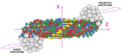
Figure 1: Schematic view of the collision. Arrows indicate the flow velocity field. The $+\hat{y}$ direction is out of the page; both the orbital angular momentum and the magnetic field point into the page.

Vorticity plays a very important role in the system evolution. Accounting for vorticity (via tuning the initial conditions and specific viscosity) it was possible to quantitatively describe the rapidity dependence of directed flow Abelev:2013cva ; Adare:2015cpn , which, at present, can not be described by any model not including initial angular momentum Csernai:2013bqa ; Bozek:2010bi ; Becattini:2015ska .

Vorticous effects may also strongly affect the baryon dynamics of the system, leading to a separation of baryon and antibaryons along the vorticity direction (perpendicular to the reaction plane) – the so-called Chiral Vortical Effect (CVE). The CVE is similar in many aspects to the more familiar Chiral Magnetic Effect (CME) - the electric charge separation along the magnetic field. For recent reviews on those and similar effects, as well as the status of the experimental search for those phenomena, see Kharzeev:2015znc ; Skokov:2016yrj . For a reliable theoretical calculation of both effects one has to know the vorticity of the created system as well as the evolution of (electro)magnetic field.

Finally, and most relevant for the present work, vorticity induces a local alignment of particles spin along its direction. The general idea that particles are polarized in peripheral relativistic heavy ion collisions along the initial (large) angular momentum of the plasma and its qualitative features were put forward more than a decade ago Liang:2004ph ; Voloshin:2004ha ; Abelev:2007zk ; Gao:2007bc ; Betz:2007kg . The idea that polarization is determined by the condition of local thermodynamic equilibrium and its quantitative link to thermal vorticity were developed in refs. Becattini:2007nd ; Becattini:2013vja . The assumption that spin degrees of freedom locally equilibrate in much the same way as momentum degrees of freedom makes it possible to provide a definite quantitative estimate of polarization through a suitable extension of the well known Cooper-Frye formula.

This phenomenon of global (that is, along the common direction of the total angular momentum) polarization has an intimate relation to the Barnett effect Barnett:1915 - magnetization by rotation - where a fraction of the orbital momentum associated with the body rotation is irreversibly transformed into the spin angular momentum of the atoms (electrons), which, on the average, point along the angular vector. Because of the proportionality between spin and magnetic moment, this tiny polarization gives rise to a finite magnetization of the rotating body, hence a magnetic field. Even closer to our case is the recent observation of the electron spin polarization in vorticous fluid Takahashi:2016 where the ”global polarization” of electron spin has been observed due to non-zero vorticity of the fluid. In condensed matter physics the gyromagnetic phenomena are often discussed on the basis of the so-called Larmor’s theorem Heims:1962 , which states that the effect of the rotation on the system is equivalent to the application of the magnetic field ${\bf B}=-\gamma^{-1}{\boldsymbol{\Omega}}$, where $\gamma$ is the particle gyromagnetic ratio.

It is worth pointing out that, however, polarization by rotation and by application of an external magnetic field are conceptually distinct effects. Particularly, the polarization by rotation is the same for particles and antiparticles, whereas polarization by magnetic field is opposite. This means that, for example, magnetization by rotation (i.e. Barnett effect) cannot be observed in a completely neutral system and the aforementioned Larmor’s theorem cannot be applied; for this purpose, an imbalance between matter and antimatter is necessary.

In this regard, the global polarization phenomenon in heavy ion collisions is peculiarly different from that observed in condensed matter physics for the density of particles and antiparticles are approximately equal, so that non-zero global polarization does not necessarily imply a magnetization. This system thus provides a unique possibility for a direct observation of the transformation of the orbital momentum into spin. Furthermore, note that in heavy ion collisions, the polarization of the particles can be directly measured via their decays (in particular via parity violating weak decays).

Calculations of global polarization in relativistic heavy ion collisions have been performed using different techniques and assumptions. Several recent calculations employ 3+1D hydrodynamic simulations and use the assumption of local thermodynamic equilibrium Becattini:2013vja ; Becattini:2015ska ; Pang:2016igs ; becakarp ; observing quite a strong dependence on the initial conditions. While local thermodynamic equilibrium for the spin degrees of freedom remains an assumption - as no estimates of the corresponding relaxation times exist - such an approach has a clear advantage in terms of simplicity of the calculations. All of the discussion below is mostly based on this assumption; to simplify the discussion even more, we will often use the non-relativistic limit.

It should be pointed out that different approaches - without local thermodynamic equilibrium - to the estimate of $\Lambda$ polarization in relativistic nuclear collisions were also proposed ayala ; celso ; Baznat:2015eca ; Aristova:2016wxe .

The paper is organized as follows: in Section II we introduce the main definitions concerning spin and polarization in a relativistic framework; in Section III we outline the thermodynamic approach to the calculation of the polarization and provide the relevant formulae for relativistic nuclear collisions; in Section IV we address the measurement of $\Lambda$ polarization and in Section V the alignment of vector mesons; finally in Section VI we discuss in detail the effect of decays on the measurement of $\Lambda$ polarization.

Notation

In this paper we use the natural units, with $\hbar=c=k_{B}=1$. The Minkowskian metric tensor is ${\rm diag}(1,-1,-1,-1)$; for the Levi-Civita symbol we use the convention $\epsilon^{0123}=1$. Operators in Hilbert space will be denoted by a large upper hat, e.g. ${\widehat{T}}$ while unit vectors with a small upper hat, e.g. $\hat{v}$.

II Spin and polarization: basic definitions

In non-relativistic quantum-mechanics, the mean spin vector is defined as:

$${\bf S}=\langle\widehat{\bf S}\rangle={\rm tr}({\widehat{\rho}}\,\widehat{\bf S})$$ (3)

where ${\widehat{\rho}}$ is the density operator of the particle under consideration and $\widehat{\bf S}$ the spin operator. The density operator can be either a pure quantum state or a mixed state, like in the case of thermodynamic equilibrium. The polarization vector is defined as the mean value of the spin operator normalized to the spin of the particle:

$${\bf P}=\langle\widehat{\bf S}\rangle/S$$ (4)

so that its maximal value is 1, that is $\|{\bf P}\|\leq 1$.

A proper relativistic extension of the spin concept, for massive particles, requires the introduction of a spin four-vector operator. This is defined as follows (see e.g. wukitung ):

$$\widehat{S}^{\mu}=-\frac{1}{2m}\epsilon^{\mu\nu\rho\lambda}\widehat{J}_{\nu\rho}\widehat{p}_{\lambda}$$ (5)

where $\widehat{J}$ and $\widehat{p}$ are the angular momentum operator and four-momentum operator of a single particle. As it can be easily shown, the spin four-vector operator commutes with the four-momentum operator (hence it is a compatible observable) and it is space-like on free particle states as it is orthogonal to the four-momentum:

$$\widehat{S}^{\mu}\widehat{p}_{\mu}=0$$ (6)

and has thus only three independent components. Particularly, in the rest frame of the particle, it has vanishing time component. Because of these properties, for single particle states with definite four-momentum $p$ it can be decomposed moussa along three spacelike vectors $n_{i}(p)$ with $i=1,2,3$ orthogonal to $p$:

$$\widehat{S}^{\mu}=\sum_{i=1}^{3}\widehat{S}_{i}(p)n_{i}(p)^{\mu}$$ (7)

It can be shown that the operators $\widehat{S}_{i}(p)$ with $i=1,2,3$ obey the well known SU(2) commutation relations and they are indeed the generators of the little group, the group of transformations leaving $p$ invariant for a massive particle. Furthermore, it is worth pointing out that $\widehat{S}^{\mu}\widehat{S}_{\mu}$ operator commutes with both momentum and spin (it is a Casimir of the full Poincaré group) and takes on the value $S(S+1)$ where $S$ is the spin of the particle over all states.

The spin and polarization four-vectors can now be defined by a straighforward extension of the eqs. (3), (4), namely:

$$S^{\mu}=\langle\widehat{S}^{\mu}\rangle\equiv{\rm tr}({\widehat{\rho}}\,\widehat{S}^{\mu})$$ (8)

and

$$P^{\mu}=\langle\widehat{S}^{\mu}\rangle/S$$ (9)

In the particle rest frame, both four-vectors have vanishing time component and effectively reduce to three-vectors. Henceforth, they will be denoted with an asterisk, that is:

$$S^{*}=(0,{\bf S}^{*})\qquad P^{*}=(0,{\bf P}^{*})$$ (10)

Obviously, they will have non-trivial transformation relations among different inertial frames, unlike in non-relativistic quantum mechanics where they are simply invariant under a galilean transformation.

For an assembly of particles, or in relativistic quantum field theory, the mean single-particle spin vector of a particle with momentum $p$ can be written:

$$S^{\mu}(p)=-\frac{1}{2m}\epsilon^{\mu\nu\rho\lambda}\frac{\sum_{\sigma}{\rm tr}\left({\widehat{\rho}}\,\widehat{J}_{\nu\rho}\widehat{p}_{\lambda}a^{\dagger}_{p,\sigma}a_{p,\sigma}\right)}{\sum_{\sigma}{\rm tr}({\widehat{\rho}}\,a^{\dagger}_{p,\sigma}a_{p,\sigma})}$$ (11)

where ${\widehat{\rho}}$ is the density operator, $\widehat{J}$ and $\widehat{p}$ are the total angular momentum and four-momentum operators, $a_{\sigma,p}$ is the destruction operator of a particle with momentum $p$ and spin component (or helicity) $\sigma$.

III The thermal approach

III.1 Non-relativistic limit

Suppose we have a non-relativistic particle at equilibrium in a thermal bath at temperature $T$ in a rotating vessel at an angular velocity $\boldsymbol{\omega}$ (corresponding to a uniform vorticity according to eq. (1) and we want to calculate its mean spin vector according to eq. (3). As spin is quantum, we have to use the appropriate density operator ${\widehat{\rho}}$ for this system at equilibrium, that in this case reads Landau:v5 ; Vilenkin:1980zv :

$${\widehat{\rho}} = \frac{1}{Z}\exp[-\widehat{H}/T+\nu{\widehat{Q}}/T+\boldsymbol{\omega}\cdot\widehat{\bf J}/T+\widehat{\boldsymbol{\mu}}\cdot{\bf B}/T]$$

$$= \frac{1}{Z}\exp[-\widehat{H}/T+\nu{\widehat{Q}}/T+\boldsymbol{\omega}\cdot(\widehat{\bf L}+\widehat{\bf S})/T+\widehat{\boldsymbol{\mu}}\cdot{\bf B}/T]]$$

where for completeness we have included a conserved charges ${\widehat{Q}}$ ($\nu$ being the corresponding chemical potentials) and a constant and uniform external magnetic field ${\bf B}$ ($\widehat{\boldsymbol{\mu}}=\mu\widehat{\bf S}/S$ being the magnetic moment). Indeed, the angular velocity $\boldsymbol{\omega}$ plays the role of a chemical potential for the angular momentum and particularly for the spin. If the constant angular velocity $\boldsymbol{\omega}$, as well as the constant magnetic field ${\bf B}$ are parallel, the above density operator can be diagonalized in the basis of eigenvectors of the spin operator component parallel to $\boldsymbol{\omega}$, $\widehat{{\bf S}}\cdot\hat{\boldsymbol{\omega}}$, thereby giving rise to a probability distribution for its different eigenvalues $m$. Specifically, the different probabilities read:

$$w[T,B,\omega](m)=\frac{\exp\left[\frac{\mu B/S+\omega}{T}m\right]}{\sum_{m=-S}^{S}\exp\left[\frac{\mu B/S+\omega}{T}m\right]}$$ (13)

The distribution eq. (13) may now be used to estimate the spin vector in eq. (3). Indeed, the only non-vanishing component of the spin vector is along the angular velocity direction; for the simpler case with $B=0$ this reads:

$${\bf S} = \hat{\boldsymbol{\omega}}\frac{\sum_{m=-S}^{S}m\exp\left[\frac{\omega}{T}m\right]}{\sum_{m=-S}^{S}\exp\left[\frac{\omega}{T}m\right]}$$ (14)

$$= \hat{\boldsymbol{\omega}}\frac{\partial}{\partial(\omega/T)}\sum_{m=-S}^{S}\exp\left[\frac{\omega}{T}m\right]$$

$$= \hat{\boldsymbol{\omega}}\frac{\partial}{\partial(\omega/T)}\frac{\sinh[(S+1/2)\omega/T]}{\sinh[\omega/2T]}$$

where $\hat{\boldsymbol{\omega}}$ is the unit vector along the direction of $\boldsymbol{\omega}$. In most circumstances, (relativistic heavy ion collisions as well) the ratio between $\omega$ and $T$ is very small and a first order expansion of the above expressions turns out to be a very good approximation. Thus, the eq. (14) becomes:

$${\bf S}\simeq\hat{\boldsymbol{\omega}}\frac{\sum_{m=-S}^{S}m^{2}\omega/T}{2S+1}=\frac{S(S+1)}{3}\frac{\boldsymbol{\omega}}{T}$$ (15)

We can now specify the polarization vector for the particles with lowest spins. For $S=1/2$ the eqs. (14) and (15) imply:

$${\bf S}=\frac{1}{2}{\bf P}=\frac{1}{2}\tanh(\omega/2T)\hat{\boldsymbol{\omega}}\simeq\frac{1}{4}\frac{\boldsymbol{\omega}}{T}\;;$$ (16)

for $S=1$:

$${\bf S}={\bf P}=\frac{2\sinh(\omega/T)}{1+2\cosh(\omega/T)}\hat{\boldsymbol{\omega}}\simeq\frac{2}{3}\frac{\boldsymbol{\omega}}{T}\;;$$ (17)

and finally, for $S=3/2$:

$${\bf S}=\frac{3}{2}{\bf P}$$

$$=\frac{(3/2)\sinh(3\omega/2T)+(1/2)\sinh(\omega/2T)}{\cosh(3\omega/2T)+\cosh(\omega/2T)}\hat{\boldsymbol{\omega}}\simeq\frac{5}{4}\frac{\boldsymbol{\omega}}{T}\;.$$ (18)

If the magnetic field is parallel to the vorticity, magnetic effects may be included by substituting:

$$\boldsymbol{\omega}\rightarrow\boldsymbol{\omega}+\mu{\bf B}/S$$ (19)

in equations (14-III.1).

III.2 Relativistic case

As it has been mentioned at the beginning of this section, all above formulae apply to the case of an individual (i.e. Boltzmann statistics) non-relativistic particle at global thermodynamic equilibrium with a constant temperature, uniform angular velocity and magnetic field. It therefore must be a good approximation when the physical conditions are not far from those, namely a non- relativistic fluid made of non-relativistic particles with a slowly varying temperature, vorticity (1) and magnetic field. However, at least in relativistic nuclear collisions, the fluid velocity is relativistic, massive particles with spin may be produced with momenta comparable to their mass, and the local relativistic vorticity - whatever it is - may not be uniform. Furthermore, there is a general issue of what is the proper relativistic extension of the angular velocity or the ratio $\omega/T$ appearing in all above formulae. The fully relativistic ideal gas with spin, in the Boltzmann approximation, at global equilibrium with rotation was studied in detail in refs. Becattini:2007nd ; Becattini:2009wh . Therein, it was found that the spin vector in the rest frame, for a particle with spin $S$ is given by:

$${\bf S}^{*}=S{\bf P}^{*}=\frac{\partial}{\partial(\omega/T)}\frac{\sinh[(S+1/2)\omega/T]}{\sinh[\omega/2T]}$$

$$\times\left[\frac{\varepsilon}{m}\hat{\boldsymbol{\omega}}-\frac{1}{m(\varepsilon+m)}(\hat{\boldsymbol{\omega}}\cdot{\bf p}){\bf p}\right]$$ (20)

where ${\bf p}$ is the momentum and $\varepsilon$ the energy of the particle in the frame where the fluid is rotating with a rigid velocity field at a constant angular velocity $\boldsymbol{\omega}$, i.e. ${\bf v}=\boldsymbol{\omega}\times{\bf x}$. It can be seen that the rest frame spin vector has a component along its momentum, unlike in the non-relativistic case, which vanishes in the low velocity limit according to the non-relativistic formula (14). Note that eq. (III.2) is derived in the approximation $\omega/T\ll m/\varepsilon$ Becattini:2007nd and the polarization is always less then unity.

The extension of these results to a fluid or a gas in a local thermodynamic equilibrium situation, such as that which is assumed to occur in the so-called hydrodynamic stage of the nuclear collision at high energy, as well as the inclusion of quantum statistics effects, requires more powerful theoretical tools. Particularly, if we want to describe the polarization of particles locally, a suitable approach requires the calculation of the quantum-relativistic Wigner function and the spin tensor. By using such an approach, the mean spin vector of $1/2$ particles with four-momentum $p$, produced around point $x$ at the leading order in the thermal vorticity was found to be Becattini:2013fla :

$$S^{\mu}(x,p)=-\frac{1}{8m}(1-n_{F})\epsilon^{\mu\rho\sigma\tau}p_{\tau}\varpi_{\rho\sigma}$$ (21)

where $n_{F}=(1+\exp[\beta(x)\cdot p-\nu(x)Q/T(x)]+1)^{-1}$ is the Fermi-Dirac distribution and $\varpi$ is given by eq. 2 at the point $x$. This equation is suitable for the situation of relativistic heavy ion collisions, where one deals with a local thermodynamic equilibrium hypersurface $\Sigma$ where hydrodynamic stage ceases and particle description sets in. It is the leading local thermodynamic equilibrium expression and it does not include dissipative corrections. It has been recovered with a different approach in ref. Fang:2016vpj . It is worth emphasizing that, according to the formula (21), thermal vorticity rather than kinematical vorticity $\partial_{\mu}u_{\nu}-\partial_{\nu}u_{\mu}$ is responsible for the mean particle spin. There is a deep theoretical reason for this: the four-vector $\beta$ in eq. (2) is a more fundamental vector for thermodynamic equilibrium in relativity than the velocity $u$ because it becomes a Killing vector field at global equilibrium Becattini:2012tc . Hence, the expansion of the equilibrium, or local equilibrium, density operator, involves $\beta$ gradients as a parameter and not the gradients of velocity and temperature separately betaframe . To illustrate this statement, it is worth mentioning that, in a relativistic rotating gas at equilibrium, with velocity field ${\bf v}=\boldsymbol{\omega}\times{\bf x}$ and $T=T_{0}/\sqrt{1-v^{2}}$, with $T_{0}$ constant, $\varpi$ is a constant, whereas the kinematical vorticity is not.

It is instructive to check that the eq. (21) yields, in the non-relativistic and global equilibrium limit, the formulae obtained in the first part of this Section. First of all, at low momentum, in eq. (21) one can keep only the term corresponding to $\tau=0$ and $p_{0}\simeq m$, so that $S^{0}\simeq 0$ and:

$$S^{\mu}(x,p)\simeq-\epsilon^{\mu\rho\sigma 0}\frac{1-n_{F}}{8}\varpi_{\rho\sigma}$$ (22)

Then, the condition of global equilibrium makes the thermal vorticity field constant and equal to the ratio of a constant angular velocity $\boldsymbol{\omega}$ and a constant temperature $T$ Becattini:2012tc that is:

$$-\frac{1}{2}\epsilon^{ijk0}\varpi_{jk}=\frac{1}{T_{0}}\omega^{i}$$ (23)

Finally, in the Boltzmann statistics limit $1-n_{F}\simeq 1$ and one finally gets the spin 3-vector as:

$${\bf S}(x,p)\simeq\frac{1}{4}\frac{\boldsymbol{\omega}}{T}$$ (24)

which is the same result as in eq. (16).

The formula (21) has another interesting interpretation: the mean spin vector is proportional to the axial thermal vorticity vector seen by the particle along its motion, that is comoving. Indeed, an antisymmetric tensor can be decomposed into two spacelike vectors, one axial and one polar, seen by an observer with velocity $u$ (the subscript c stands for comoving):

$$\varpi_{\rm c}^{\mu}=-\frac{1}{2}\epsilon^{\mu\rho\sigma\tau}\varpi_{\rho\sigma}u_{\tau}\qquad\alpha_{\rm c}^{\mu}=\varpi^{\mu\nu}u_{\nu}$$ (25)

in much the same way as the electromagnetic field tensor $F_{\mu\nu}$ can be decomposed into a comoving electric and magnetic field. Thus, the eq. (21) can be rewritten as:

$$S^{\mu}(x,p)=\frac{1}{4}(1-n_{F})\varpi_{\rm c}^{\mu}$$ (26)

like in the non-relativistic case, provided that $\varpi_{\rm c}^{\mu}$ is the thermal vorticity axial vector in the particle comoving frame.

To get the experimentally observable quantity, that is the spin vector of some particle species as a function of the four-momentum, one has to integrate the above expressions over the particlization hypersurface $\Sigma$:

$$S^{\mu}(p)=\frac{\int d\Sigma_{\lambda}p^{\lambda}f(x,p)S^{\mu}(x,p)}{\int d\Sigma_{\lambda}p^{\lambda}f(x,p)}$$ (27)

The mean spin vector i.e. averaged over momentum, of some $S=1/2$ particle species, can be then expressed as:

$$S^{\mu}=\frac{1}{N}\int\frac{{\rm d}^{3}{\rm p}}{p^{0}}\int d\Sigma_{\lambda}p^{\lambda}n_{F}(x,p)S^{\mu}(x,p)$$ (28)

where $N=\int\frac{{\rm d}^{3}{\rm p}}{p^{0}}\int d\Sigma_{\lambda}p^{\lambda}n_{F}(x,p)$ is the average number of particles produced at the particlization surface. One can also derive the expression of the spin vector in the rest frame from (28) taking into account Lorentz invariance of most of the factors in it:

$$S^{*\mu}=\frac{1}{N}\int\frac{{\rm d}^{3}{\rm p}}{p^{0}}\int d\Sigma_{\lambda}p^{\lambda}n_{F}(x,p)S^{*\mu}(x,p)$$ (29)

Looking at the eq. (26), one would say that a measurement of the mean spin vector provides an estimate of the mean comoving thermal vorticity axial vector.

As has been mentioned, the formula (21) applies to spin $1/2$ particles. However, a very plausible extension to higher spins can be obtained by comparing the global equilibrium expression (III.2) for particles with spin $S$ in the Boltzmann statistics, with the first-order expansion in the thermal vorticity for spin $1/2$ eq. (21). Taking into account that the thermal vorticity should replace $\omega/T$ and the $\omega/T\ll 1$ expansion in eq. (15), one obtains, in the Boltzmann limit:

$$S^{\mu}(x,p)\simeq-\frac{1}{2m}\frac{S(S+1)}{3}\epsilon^{\mu\rho\sigma\tau}p_{\tau}\varpi_{\rho\sigma}$$ (30)

and the corresponding integrations over the hypersurface $\Sigma$ and momentum similar to eqs. (27) and (28).

Finally, we would like to mention that the formula (30) could be naturally extended to include the electromagnetic field by simply replacing $\varpi_{\rho\sigma}$ with $\varpi_{\rho\sigma}+\mu F_{\rho\sigma}/S$, in agreement with the non-relativistic distribution in eq. (III.1).

$$S^{\mu}(x,p)\simeq-\frac{1}{2m}\frac{S(S+1)}{3}\epsilon^{\mu\rho\sigma\tau}p_{\tau}\left(\varpi_{\rho\sigma}-\frac{\mu}{S}F_{\rho\sigma}\right)$$ (31)

and, by using the comoving axial thermal vorticity vector and the comoving magnetic field:

$$S^{\mu}(x,p)\simeq\frac{S(S+1)}{3}\left(\varpi_{\rm c}^{\mu}+\frac{\mu}{S}B_{\rm c}^{\mu}\right)$$ (32)

IV $\Lambda$ polarization measurement

The most straightforward way to detect a global polarization in relativistic nuclear collisions is focussing on $\Lambda$ hyperons. As they decay weakly violating parity, in the $\Lambda$ rest frame the daughter proton is predominantly emitted along the $\Lambda$ polarization:

$$\frac{dN}{d\Omega^{*}}=\frac{1}{4\pi}\left(1+\alpha_{\Lambda}{\bf P}^{*}_{\Lambda}\cdot\hat{{\bf p}}^{*}\right),$$ (33)

where $\alpha_{\Lambda}=-\alpha_{\bar{\Lambda}}\approx 0.642$ is the $\Lambda$ decay constant Agashe:2014kda . $\hat{{\bf p}}^{*}$ is the unit vector along the proton momentum and ${\bf P}^{*}$ the polarization vector of the $\Lambda$, both in $\Lambda$’s rest frame.

For a global polarization measurement, one also needs to know the direction of the total angular momentum, along which the local thermal vorticity will be preferentially aligned. This direction can be reconstructed by measuring the directed flow of the projectile spectators (which conventionally is taken as a positive $x$ direction in the description of any anisotropic flow Voloshin:2008dg ). Recently it was shown that spectators, on average, deflect outward from the centerline of the collision Voloshin:2016ppr . Thus, measuring this deflection provides information about the orientation of the nuclei during the collision (i.e. the impact parameter $\mathbf{b}$) and the direction of the angular momentum. One can also use for this purpose the flow of produced particles if their relative orientation with respect to the spectator flow is known. For heavy ion collisions the direction of the system orbital momentum on average coincides with the direction of the magnetic field.

Finally, because the reaction plane angle can not be reconstructed exactly in experiments, one has to correct for the reaction plane resolution. In order to apply the standard flow methods for such a correction, it is convenient first to ’project’ the distribution eq.33 on the transverse plane, restricting the analysis to the difference in azimuths of the proton emission and that of the reaction plane. One arrives at Abelev:2007zk :

$$P_{\Lambda}=\frac{8}{\pi\alpha_{\Lambda}}\frac{\left\langle\sin(\Psi_{\rm EP}^{(1)}-\phi_{p}^{*})\right\rangle}{R^{(1)}_{\rm EP}},$$ (34)

where $\Psi_{\rm EP}^{(1)}$ is the first harmonic (directed flow) event plane (e.g. determined by the deflection of projectile spectators) and $R^{(1)}_{\rm EP}$ is the corresponding event plane resolution (see Ref. Abelev:2007zk for the discussion of the detector acceptance effects).

It should be pointed out that in relativistic heavy ion collisions the electromagnetic field may also play a role in determining the polarization of produced particles. If we keep the assumption of local thermodynamic equilibrium, one can apply the formulae (31), (32). However, as yet, it is not clear if the spin degrees of freedom will respond to a variation of thermal vorticity as quickly as to a variation of the electromagnetic field. If the relaxation times were sizeably different, one would estimate thermal vorticity and magnetic field from the measured polarization (see Section VI) at different times in the process. The magnetic moments of particles and antiparticles have opposite signs, so the effect of the electromagnetic field is a splitting in global polarization of particles and antiparticles. Particularly, the $\Lambda$ magnetic moment is $\mu_{\Lambda}\approx-0.61\mu_{N}=-0.61e/(2m_{p})$ Agashe:2014kda and, under the assumption above, one can take advantage of a difference in the polarization of primary $\Lambda$s and $\bar{\Lambda}$s (i.e. those emitted directly at hadronization) to estimate the (mean comoving) magnetic field:

$$eB\approx-\Delta P^{\rm prim}m_{p}T/0.61$$ (35)

where $m_{p}$ is the proton mass, and $\Delta P^{\rm prim}\equiv P^{\rm prim}_{\Lambda}-P^{\rm prim}_{\overline{\Lambda}}$ is the difference in polarization of primary $\Lambda$ and $\overline{\Lambda}$. An (absolute) difference in the polarization of primary $\Lambda$’s of of 0.1% then would correspond to a magnetic field of the order of $\sim 10^{-2}m_{\pi}^{2}$, well within the range of theoretical estimates Tuchin:2014hza ; Gursoy:2014aka ; McLerran:2013hla . However, we warn that equation 35 should not be applied to experimental measurements without a detailed accounting for polarized feed-down effects, which are discussed in Section VI.

Finally, we note that a small difference between $\Lambda$ and $\bar{\Lambda}$ polarization could also be due to the finite baryon chemical potential making the factor $(1-n_{F})$ in eq. (21) different for particles and antiparticles; this Fermi statistics effect might be relevant only at low collision energies.

V Spin alignment of vector mesons

The global polarization of vector mesons, such as $\phi$ or $K^{*}$, can be accessed via the so-called spin alignment Liang:2004xn ; Abelev:2008ag . Parity is conserved in the strong decays of those particles and, as a consequence, the daughter particle distribution is the same for the states $S_{z}=\pm 1$. In fact, it is different for the state $S_{z}=0$, and this fact can be used to determine a polarization of the parent particle. By referring to eq. (13), in the thermal approach the deviation of the probability for the state $S_{z}=0$ from 1/3, is only of the second order in $\varpi$:

$$p_{0}=\frac{1}{1+2\cosh\varpi_{\rm c}}\approx\frac{1}{3+\varpi_{\rm c}^{2}}\approx\frac{1}{3}(1-\varpi_{\rm c}^{2}/3),$$ (36)

which could make this measurement difficult. Similarly difficult will be the detection of the global polarization with the help of other strong decay channels, e.g. proposed in Ref. Shuryak:2016hor .

VI Accounting for decays

According to eq. (31) (or, in the non-relativistic limit, equations 15-III.1), the polarization of primary $\Lambda$ hyperons provides a measurement of the (comoving) thermal vorticity and the (comoving) magnetic field of the system that emits them. However, only a fraction of all detected $\Lambda$ and $\bar{\Lambda}$ hyperons are produced directly at the hadronization stage and are thus primary. Indeed, a large fraction thereof stems from decays of heavier particles and one should correct for feed-down from higher-lying resonances when trying to extract information about the vorticity and the magnetic field from the measurement of polarization. Particularly, the most important feed-down channels involve the strong decays of $\Sigma^{*}\rightarrow\Lambda+\pi$, the electromagnetic decay $\Sigma^{0}\rightarrow\Lambda+\gamma$, and the weak decay $\Xi\rightarrow\Lambda+\pi$.

Decay	$C$
parity-conserving:  $\nicefrac{{1}}{{2}}^{+}\to\nicefrac{{1}}{{2}}^{+}\;\;0^{-}$	$-1/3$
parity-conserving:  $\nicefrac{{1}}{{2}}^{-}\to\nicefrac{{1}}{{2}}^{+}\;\;0^{-}$	1
parity-conserving:  $\nicefrac{{3}}{{2}}^{+}\to\nicefrac{{1}}{{2}}^{+}\;\;0^{-}$	$1/3$
parity-conserving:  $\nicefrac{{3}}{{2}}^{-}\to\nicefrac{{1}}{{2}}^{+}\;\;0^{-}$	$-1/5$
$\Xi^{0}\rightarrow\Lambda+\pi^{0}$	+0.900
$\Xi^{-}\rightarrow\Lambda+\pi^{-}$	+0.927
$\Sigma^{0}\rightarrow\Lambda+\gamma$	-1/3

Table 1: Polarization transfer factors $C$ (see eq. (37)) for important decays $X\to\Lambda(\Sigma)\pi$

When polarized particles decay, their daughters are themselves polarized because of angular momentum conservation. The amount of polarization which is inherited by the daughter particle, or transferred from the parent to the daughter, in general depends on the momentum of the daughter in the rest frame of the parent. As long as one is interested in the mean, momentum-integrated, spin vector in the rest frame, a simple linear rule applies (see Appendix A), that is:

$${\bf S}^{*}_{D}=C{\bf S}^{*}_{P}$$ (37)

where $P$ is the parent particle, $D$ the daughter and $C$ a coefficient whose expression (see Appendix A) may or may not depend on the dynamical amplitudes. In many two-body decays, the conservation laws constrain the final state to such an extent that the coefficient $C$ is independent of the dynamical matrix elements. This happens, e.g., in the strong decay $\Sigma^{*}(1385)\to\Lambda\pi$ and the electromagnetic $\Sigma^{0}\to\Lambda\gamma$ decay, whereas it does not in $\Xi\to\Lambda\pi$ decays, which is a weak decay.

If the decay products have small momenta compared to their masses, one would expect that the spin transfer coefficient $C$ was determined by the usual quantum-mechanical angular momentum addition rules and Clebsch-Gordan coefficients, as the spin vector would not change under a change of frame. Surprisingly, this holds in the relativistic case provided that the coefficient $C$ is independent of the dynamics, as it is shown in Appendix A. In this case, $C$ is independent of Lorentz factors $\beta$ or $\gamma$ of the daughter particles in the rest frame of the parent, unlike naively expected. This feature makes $C$ a simple rational number in all cases where the conservation laws fully constrain it. The polarization transfer coefficients $C$ of several important baryons decaying to $\Lambda$s are reported in table (1) and their calculation described in detail in Appendix A.

Taking the feed-down into account, the measured mean $\Lambda$ spin vector along the angular momentum direction can then be expressed as:

$${\bf S}^{*,{\rm meas}}_{\Lambda}=\sum_{R}\left[f_{\Lambda R}C_{\Lambda R}-\tfrac{1}{3}f_{\Sigma^{0}R}C_{\Sigma^{0}R}\right]{\bf S}^{*}_{R}.$$ (38)

This formula accounts for direct feed-down of a particle-resonance $R$ to a $\Lambda$, as well as the two-step decay $R\rightarrow\Sigma^{0}\rightarrow\Lambda$; these are the only significant feed-down paths to a $\Lambda$. In the eq.( 38), $f_{\Lambda R}$ ($f_{\Sigma^{0}R}$) is the fraction of measured $\Lambda$’s coming from $R\rightarrow\Lambda$ ($R\rightarrow\Sigma^{0}\rightarrow\Lambda$). The spin transfer to the $\Lambda$ in the direct decay is denoted $C_{\Lambda R}$, while $C_{\Sigma^{0}R}$ represents the spin transfer from $R$ to the daughter $\Sigma^{0}$. The explicit factor of $-\tfrac{1}{3}$ is the spin transfer coefficient from the $\Sigma^{0}$ to the daughter $\Lambda$ from the decay $\Sigma^{0}\rightarrow\Lambda+\gamma$.

In terms of polarization (see eq. (15)):

$$P^{\rm meas}_{\Lambda}=2\sum_{R}\left[f_{\Lambda R}C_{\Lambda R}-\tfrac{1}{3}f_{\Sigma^{0}R}C_{\Sigma^{0}R}\right]S_{R}P_{R}$$ (39)

where $S_{R}$ is the spin of the particle $R$. The sums in equations (38) and (39) are understood to include terms for the contribution of primary $\Lambda$s and $\Sigma^{0}$s. These equations are readily extended to include additional multiple-step decay chains that terminate in a $\Lambda$ daughter, although such contributions would be very small.

Therefore, in the limit of small polarization, the polarizations of measured (including primary as well as secondary) $\Lambda$ and $\overline{\Lambda}$ are linearly related to the mean (comoving) thermal vorticity and magnetic field according to eq. (32) or eq. (15), and these physical quantities may be extracted from measurement as:

$$\left(\begin{array}[]{c}\varpi_{\rm c}\\[25.0pt] B_{\rm c}/T\end{array}\right)=\left[\begin{array}[]{l l}\frac{2}{3}\sum\limits_{R}\left(f_{\Lambda R}\,C_{\Lambda R}-\frac{1}{3}f_{\Sigma^{0}R}\,C_{\Sigma^{0}R}\right)\,S_{R}(S_{R}+1)&\quad\frac{2}{3}\sum\limits_{R}\left(f_{\Lambda R}\,C_{\Lambda R}-\frac{1}{3}f_{\Sigma^{0}R}\,C_{\Sigma^{0}R}\right)\,(S_{R}+1)\,\mu_{R}\\[20.0pt] \frac{2}{3}\sum\limits_{\overline{R}}\left(f_{\overline{\Lambda}\overline{R}}\,C_{\overline{\Lambda}\overline{R}}-\frac{1}{3}f_{\overline{\Sigma}^{0}\overline{R}}\,C_{\overline{\Sigma}^{0}\overline{R}}\right)\,S_{\overline{R}}(S_{\overline{R}}+1)&\quad\frac{2}{3}\sum\limits_{\overline{R}}\left(f_{\overline{\Lambda}\overline{R}}\,C_{\overline{\Lambda}\overline{R}}-\frac{1}{3}f_{\overline{\Sigma}^{0}\overline{R}}\,C_{\overline{\Sigma}^{0}\overline{R}}\right)\,(S_{\overline{R}}+1)\,\mu_{\overline{R}}\end{array}\right]^{{-1}}\left(\begin{array}[]{c}P^{\rm meas}_{\Lambda}\\[20.0pt] P^{\rm meas}_{\overline{\Lambda}}\\[5.0pt] \end{array}\right).$$ (40)

In the eq. (40), $\overline{R}$ stands for antibaryons that feed down into measured $\overline{\Lambda}$s. The polarization transfer is the same for baryons and antibaryons ($C_{\overline{\Lambda R}}=C_{\Lambda R}$) and the magnetic moment has opposite sign ($\mu_{\overline{R}}=-\mu_{R}$).

According to the THERMUS model Wheaton:2004qb , tuned to reproduce semi-central Au+Au collisions at $\sqrt{s_{\rm NN}}=19.6$ GeV, fewer than 25% of measured $\Lambda$s and $\overline{\Lambda}$s are primary, while more than 60% may be attributed to feed-down from primary $\Sigma^{*}$, $\Sigma^{0}$ and $\Xi$ baryons.

The remaining $\sim 15\%$ come from small contributions from a large number higher-lying resonances such as $\Lambda(1405),\Lambda(1520),\Lambda(1600),\Sigma(1660)$ and $\Sigma(1670)$. We find that, for $B=0$, their contributions to the measured $\Lambda$ polarization largely cancel each other, due to alternating signs of the polarization transfer factors. Their net effect, then, is essentially a 15% “dilution,” contributing $\Lambda$s to the measurement with no effective polarization. Since the magnetic moments of these baryons are unmeasured, it is not clear what their contribution to $P_{\Lambda{\rm meas}}$ would be when $B\neq 0$. However, it is reasonable to assume it would be small, as the signs of both the transfer coefficients and the magnetic moments will fluctuate.

Accounting for feed-down is crucial for quantitative estimates of vorticity and magnetic field based on experimental measurements of the global polarization of hyperons, as we illustrate with an example, using $\sqrt{s_{\rm NN}}=19.6$ GeV THERMUS feed-down probabilities. Let us assume that the thermal vorticity is $\varpi=0.1$ and the magnetic field is $B=0$. In this case, according to eq. (16), the primary hyperon polarizations are $P^{\rm prim}_{\Lambda}=P^{\rm prim}_{\overline{\Lambda}}=0.05$. However, the measured polarizations would be $P^{\rm meas}_{\Lambda}=0.0395$ and $P^{\rm meas}_{\overline{\Lambda}}=0.0383$. The two measured values differ because the finite baryochemical potential at these energies leads to slightly different feed-down fractions for baryons and anti-baryons.

Hence, failing to account for feed-down when using equation 16 would lead to a $\sim 20\%$ underestimate of the thermal vorticity. Even more importantly, if the splitting between $\Lambda$ and $\overline{\Lambda}$ polarizations were attributed entirely to magnetic effects (i.e. if one neglected to account for feed-down effects), equation (35) would yield an erroneous estimate $B\approx-0.015m_{\pi}^{2}$. This erroneous estimate has roughly the magnitude of the magnetic field expected in heavy ion collisions, but points the in the “wrong” direction, i.e. opposite the vorticity. In other words, in the absence of feed-down effects, a magnetic field is expected to cause $P_{\overline{\Lambda}}>P_{\Lambda}$, whereas feed-down in the absence of a magnetic field will produce a splitting of the opposite sign.

VII Summary and conclusions

The nearly-perfect fluid generated in non-central heavy ion collisions is characterized by a huge vorticity and magnetic field, both of which can induce a global polarization of the final hadrons. Conversely, a measurement of polarization makes it possible to estimate the thermal vorticity as well as the electromagnetic field developed in the plasma stage of the collision. As the thermal vorticity appears to be strongly dependent on the hydrodynamic initial conditions, polarization is a very sensitive probe of the QGP formation process. Pinning down (thermal) vorticity and magnetic field is also very important for the quantitative assessment of thus-far unobserved QCD effects, such as the chiral magnetic and chiral vortical effects.

We have summarized and elucidated the thermal approach to the calculation of the polarization of particles in relativistic heavy ion collisions, based on the assumption of local thermodynamic equilibrium of the spin degrees of freedom at hadronization. We have put forward an extension of the formulae for spin $\nicefrac{{1}}{{2}}$ particles to particles with any spin, with an educated guess based on the global equilibrium case. The extension to any spin is needed to account for feed-down contributions that are crucial to make a proper estimate of the polarization at the hadronization stage.

We have discussed in detail how polarization is transferred to the decay products in a decay process and shown that a simple linear propagation rule applies to the momentum-averaged rest-frame spin vectors. We have developed the general formulae for the polarization transfer coefficients in two-body decays and carried out the explicit calculations for the most important decays involving a $\Lambda$ hyperon. We have shown how to take the decays into account for the extraction of thermal vorticity and magnetic field. It should be stressed, though, that the extraction of such quantities at hadronization relies on the aforementioned assumption of local thermodynamic equilibrium; it is still unclear whether this is correct for the electromagnetic field term.

The feed-down corrections can be significant, reducing the measured polarizations by $\sim 20\%$, as compared to the polarization of primary particles at RHIC energies. More importantly, feed-down may generate a splitting between measured $\Lambda$ and $\overline{\Lambda}$ polarizations of roughly the same magnitude as the splitting expected from magnetic effects. Fortunately, at finite baryochemical potential, the two splittings have opposite sign, so that feed-down effects should not “artificially” mock up magnetic effects.

Finally, it must be pointed out that there is a further effect, in fact much harder to assess, which can affect the reconstruction of the polarization of primary particles, that is post-hadronization interactions. Indeed, hadronic elastic interaction may involve a spin flip which, presumably, randomizes the spin direction of primary as well as secondary particles, thus decreasing the estimated mean global polarization.

Appendix A Polarization transfer in two-body decay

We want to calculate the polarization which is inherited by the $\Lambda$ hyperons in decays of polarized higher lying states and, particularly, $\Sigma^{*}\rightarrow\Lambda\pi$, $\Sigma^{0}\rightarrow\Lambda\gamma$ and $\Xi\rightarrow\Lambda\pi$. The goal is to determine the mean spin vector in the $\Lambda$ rest frame, as a function of the mean spin vector of the decaying particle in its rest frame. We will finally show that the equation (37) applies and we will determine the exact expression of the coefficient $C$.

We will work out the exact relativistic result. In a relativistic framework, the use of the helicity basis is very convenient; for a complete description of the helicity and alternative spin formalisms, we refer the reader to refs. moussa ; wukitung ; chung For a particle with spin $J$ and spin projection along the $z$ axis $M$ in its rest frame (in the rest frame helicity coincides with the eigenvalue of the spin operators $\widehat{S}$, conventionally $\widehat{S}_{3}$, see text) decaying into two particles $A$ and $B$, the final state $|\psi\rangle$ can be written as a superposition of states with definite momentum and helicities:

$$|\psi\rangle\propto\sum_{\lambda_{A},\lambda_{B}}\int{\rm d}\Omega\;D^{J}(\varphi,\theta,0)^{M*}_{\lambda}|{\bf p},\lambda_{A},\lambda_{B}\rangle T^{J}(\lambda_{A},\lambda_{B})$$ (41)

where ${\bf p}$ is the momentum of either particle, $\theta$ and $\varphi$ its spherical coordinates ${\rm d}\Omega=\sin\theta{\rm d}\theta{\rm d}\varphi$ the corresponding infinitesimal solid angle, $D^{J}$ is the Wigner rotation matrix in the representation of spin $J$, $T^{J}(\lambda_{A},\lambda_{B})$ are the reduced dynamical amplitudes depending only on the final helicities and:

$$\lambda=\lambda_{A}-\lambda_{B}$$

The mean relativistic spin vector of, e.g., the particle $A$ after the decay is given by:

$$S^{\mu}=\langle\psi|\widehat{S}_{A}^{\mu}|\psi\rangle$$

with $\langle\psi|\psi\rangle=1$, hence:

$$S^{\mu} = \sum_{\lambda_{A},\lambda_{B},\lambda^{\prime}_{A}}\int{\rm d}\Omega\;D^{J}(\varphi,\theta,0)^{M*}_{\lambda}D^{J}(\varphi,\theta,0)^{M}_{\lambda^{\prime}}$$ (42)

$$\times \langle\lambda^{\prime}_{A}|\widehat{S}_{A}^{\mu}|\lambda_{A}\rangle T^{J}(\lambda_{A},\lambda_{B})T^{J}(\lambda^{\prime}_{A},\lambda_{B})^{*}$$

$$\times \left({\sum_{\lambda_{A},\lambda_{B}}\int{\rm d}\Omega\;|D^{J}(\varphi,\theta,0)^{M*}_{\lambda}|^{2}|T^{J}(\lambda_{A},\lambda_{B})|^{2}}\right)^{-1}$$

$$= \sum_{\lambda_{A},\lambda_{B},\lambda^{\prime}_{A}}\int{\rm d}\Omega\;D^{J}(\varphi,\theta,0)^{M*}_{\lambda}D^{J}(\varphi,\theta,0)^{M}_{\lambda^{\prime}}$$

$$\times \langle\lambda^{\prime}_{A}|\widehat{S}_{A}^{\mu}|\lambda_{A}\rangle T^{J}(\lambda_{A},\lambda_{B})T^{J}(\lambda^{\prime}_{A},\lambda_{B})^{*}$$

$$\times \left(\frac{4\pi}{2J+1}{\sum_{\lambda_{A},\lambda_{B}}|T^{J}(\lambda_{A},\lambda_{B})|^{2}}\right)^{-1}$$

where we have used the known integrals of the Wigner $D$ matrices and the fact that the operator $\widehat{S}_{A}$ does not change the momentum eigenvalues as well as the helicity of the particle $B$. This operator can be decomposed as in eq. (7), with $n_{i}(p)$ being three spacelike unit vectors orthogonal to the four-momentum $p$. They can be obtained by applying the so-called standard Lorentz transformation $[p]$ turning the unit time vector $\hat{t}$ into the direction of the four-momentum $p$ moussa , to the three space axis vectors ${\bf e}_{i}$, namely:

$$n_{i}(p)=[p]({\bf e}_{i})$$

so that (we have temporarily dropped the subscript $A$ for the sake of simplicity):

$$\widehat{S}=\sum_{i}\widehat{S}_{i}n_{i}(p)=[p](\sum_{i}\widehat{S}_{i}{\bf e}_{i})$$ (43)

by taking advantage of the linearity of $[p]$. It is convenient to rewrite the sum in the argument of $[p]$ along the spherical vector basis $e_{+},e_{-},e_{0}$ which is used to define the $D^{J}$ matrix elements:

$${\bf e}_{+} = -\frac{1}{\sqrt{2}}({\bf e}_{1}+i{\bf e}_{2})$$

$${\bf e}_{-} = \frac{1}{\sqrt{2}}({\bf e}_{1}-i{\bf e}_{2})$$

$${\bf e}_{0} = {\bf e}_{3}$$

so that:

$$\sum_{i}\widehat{S}_{i}{\bf e}_{i}=-\frac{1}{\sqrt{2}}\widehat{S}_{-}{\bf e}_{+}+\frac{1}{\sqrt{2}}\widehat{S}_{+}{\bf e}_{-}+\widehat{S}_{0}{\bf e}_{0}$$ (44)

where $\widehat{S}_{\pm}=\widehat{S}_{1}\pm i\widehat{S}_{2}$ are the familiar ladder operators. With these operators, we can now easily calculate the spin matrix elements in eq. (42) because their action onto helicity kets $|\lambda\rangle$ is precisely the familiar one onto eigenstates of the $z$ projection of angular momentum with eigenvalue $\lambda$, e.g.:

$$\langle\lambda^{\prime}|\widehat{S}_{0}|\lambda\rangle=\lambda\delta_{\lambda,\lambda^{\prime}}$$

and in general, using eqs. (43) and (44), we can write:

$$\langle\lambda^{\prime}_{A}|\widehat{S}_{A}|\lambda_{A}\rangle=\sum_{n=-1}^{1}a_{n}\langle\lambda^{\prime}_{A}|\widehat{S}_{A,-n}|\lambda_{A}\rangle[p]({\bf e}_{n})$$ (45)

where $a_{n}=-n/\sqrt{2}+\delta_{n,0}$.

To work out the eq. (45), we need to find an expression of the standard transformation $[p]$. In principle, it can be freely chosen, but the choice which makes $\lambda$ the particle helicity weinberg ; chung is the composition of a Lorentz boost along the $z$ axis of hyperbolic angle $\xi$ such that $\sinh\xi=\|{\bf p}\|/m$, followed by a rotation around the $y$ axis of angle $\theta$ and a rotation around the $z$ axis by an angle $\varphi$ (see above):

$$[p]={\sf R}_{z}(\varphi){\sf R}_{y}(\theta){\sf L}_{z}(\xi)$$

Thus:

$$[p]({\bf e}_{\pm}) = {\sf R}_{z}(\varphi){\sf R}_{y}(\theta){\sf L}_{z}(\xi)({\bf e}_{\pm})$$

$$= {\sf R}_{z}(\varphi){\sf R}_{y}(\theta)({\bf e}_{\pm})=\sum_{l=-1}^{1}D^{1}(\varphi,\theta,0)^{l}_{\pm 1}{\bf e}_{l}$$

because $e_{\pm}$ is invariant under a boost along the $z$ axis. Conversely, ${\bf e}_{0}$ is not invariant under the Lorentz boost and:

$$[p]({\bf e}_{0}) = \cosh\xi{\sf R}_{z}(\varphi){\sf R}_{y}(\theta)({\bf e}_{0})+\sinh\xi{\sf R}_{z}(\varphi){\sf R}_{y}(\theta)(\hat{t})$$

$$= \sum_{l=-1}^{1}\frac{\varepsilon}{m}D^{1}(\varphi,\theta,0)^{l}_{0}{\bf e}_{l}+\frac{\rm p}{m}\hat{t}$$

where ${\rm p})=\|{\bf p}\|$, $\varepsilon=\sqrt{{\rm p}^{2}+m^{2}}$ is the energy and $\hat{t}$ is the unit vector in the time direction. We can now plug the above two equations into the eq. (45) to get:

$$\langle\lambda^{\prime}_{A}|\widehat{S}_{A}|\lambda_{A}\rangle=\sum_{l,n}b_{n}D^{1}(\varphi,\theta,0)^{l}_{n}\langle\lambda^{\prime}_{A}|\widehat{S}_{A,-n}|\lambda_{A}\rangle{\bf e}_{l}$$

$$+\lambda_{A}\delta_{\lambda_{A},\lambda^{\prime}_{A}}\frac{\rm p}{m}\hat{t}$$ (46)

where $b_{n}=-n/\sqrt{2}+\gamma\delta_{n,0}$ with $\gamma=\varepsilon/m$ the Lorentz factor of the decayed particle $A$ in the rest frame of the decaying particle.

We can now write down the fully expanded expression of the mean spin vector $S$ in eq. (42). The time component is especially simple; by using the eq. (A) one has:

$$S^{0} = \frac{\rm p}{m}\sum_{\lambda_{A},\lambda_{B}}\lambda_{A}\int{\rm d}\Omega\;|D^{J}(\varphi,\theta,0)^{M*}_{\lambda}|^{2}|T^{J}(\lambda_{A},\lambda_{B})|^{2}$$ (47)

$$\times \left(\frac{4\pi}{2J+1}{\sum_{\lambda_{A},\lambda_{B}}|T^{J}(\lambda_{A},\lambda_{B})|^{2}}\right)^{-1}$$

and after integrating over $\Omega$:

$$S^{0}=\frac{\rm p}{m}\frac{\sum_{\lambda_{A},\lambda_{B}}\lambda_{A}|T^{J}(\lambda_{A},\lambda_{B})|^{2}}{\sum_{\lambda_{A},\lambda_{B}}|T^{J}(\lambda_{A},\lambda_{B})|^{2}}$$ (48)

Similarly, the space component reads:

$${\bf S}=\!\!\!\!\sum_{\lambda_{A},\lambda_{B},\lambda^{\prime}_{A}}\!\!\!T^{J}(\lambda_{A},\lambda_{B})T^{J}(\lambda^{\prime}_{A},\lambda_{B})^{*}\sum_{n,l}\langle\lambda^{\prime}_{A}|\widehat{S}_{A,-n}|\lambda_{A}\rangle$$

$$\times b_{n}\int{\rm d}\Omega\;D^{J}(\varphi,\theta,0)^{M*}_{\lambda}D^{J}(\varphi,\theta,0)^{M}_{\lambda^{\prime}}D^{1}(\varphi,\theta,0)^{l}_{n}{\bf e}_{l}$$

$$\times\left(\frac{4\pi}{2J+1}{\sum_{\lambda_{A},\lambda_{B}}|T^{J}(\lambda_{A},\lambda_{B})|^{2}}\right)^{-1}$$ (49)

We note that the integrands in the angular variables $\theta,\varphi$ in both eqs. (47) and (A) are proportional to the mean relativistic spin vector at some momentum ${\bf p}$, that is $S(p)$. The angular integrals in the eq. (A) are known and can be expressed in terms of Clebsch-Gordan coefficients:

$${\bf S}=\!\!\!\!\sum_{\lambda_{A},\lambda_{B},\lambda^{\prime}_{A}}\!\!\!T^{J}(\lambda_{A},\lambda_{B})T^{J}(\lambda^{\prime}_{A},\lambda_{B})^{*}\sum_{n,l}\langle\lambda^{\prime}_{A}|\widehat{S}_{A,-n}|\lambda_{A}\rangle$$

$$\!\!\!\times b_{n}\langle JM|J1|Ml\rangle\langle J\lambda|J1|\lambda^{\prime}n\rangle{\bf e}_{l}\left({\sum_{\lambda_{A},\lambda_{B}}|T^{J}(\lambda_{A},\lambda_{B})|^{2}}\right)^{-1}$$

$$\!\!\!=\sum_{\lambda_{A},\lambda_{B},\lambda^{\prime}_{A}}\!\!\!T^{J}(\lambda_{A},\lambda_{B})T^{J}(\lambda^{\prime}_{A},\lambda_{B})^{*}\sum_{n}\langle\lambda^{\prime}_{A}|\widehat{S}_{A,-n}|\lambda_{A}\rangle$$

$$\!\!\!\times b_{n}\langle JM|J1|M0\rangle\langle J\lambda|J1|\lambda^{\prime}n\rangle{\bf e}_{0}\left({\sum_{\lambda_{A},\lambda_{B}}|T^{J}(\lambda_{A},\lambda_{B})|^{2}}\right)^{-1}$$

Note that the only non-vanishing spatial component of the mean relativistic spin vector is the along the $z$ axis, being proportional to ${\bf e}_{0}={\bf e}_{3}$. This is a result of rotational invariance, as the decaying particle is polarized along this axis by construction.

What we have calculated so far is the mean relativistic spin vector in the decaying particle rest frame. However, one is also interested in the same vector in the decayed (that is $A$) particle rest frame. For some momentum ${\bf p}$, it can be obtained by means of a Lorentz boost:

$${\bf S}^{*}(p)={\bf S}(p)-\frac{{\bf p}}{\varepsilon(\varepsilon+m)}{\bf S}(p)\cdot{\bf p}$$

Since ${\bf S}(p)\cdot{\bf p}=S^{0}(p)\varepsilon$ as $S$ is a four-vector orthogonal to $p$, we can obtain the mean, i.e. momentum integrated, vector:

$${\bf S}^{*}=\langle{\bf S}^{*}(p)\rangle=\langle{\bf S}(p)\rangle-\frac{1}{\varepsilon+m}\langle{\bf p}S^{0}(p)\rangle$$

$$={\bf S}-\frac{1}{\varepsilon+m}\langle{\bf p}S^{0}(p)\rangle$$ (51)

The first term on the right hand side is the vector in eq. (A), while for the second term we have, from eq. (47) and using:

$${\bf p}={\rm p}\sum_{l=-1}^{1}D^{1}(\varphi,\theta,0)^{l}_{0}{\bf e}_{l}$$

$$\langle{\bf p}S^{0}(p)\rangle=\frac{{\rm p}^{2}}{m}\sum_{\lambda_{A},\lambda_{B}}\lambda_{A}|T^{J}(\lambda_{A},\lambda_{B})|^{2}\sum_{l=-1}^{1}{\bf e}_{l}$$

$$\times\int{\rm d}\Omega\;|D^{J}(\varphi,\theta,0)^{M*}_{\lambda}|^{2}D^{1}(\varphi,\theta,0)^{l}_{0}$$

$$\times\left(\frac{4\pi}{2J+1}{\sum_{\lambda_{A},\lambda_{B}}|T^{J}(\lambda_{A},\lambda_{B})|^{2}}\right)^{-1}$$

$$=\frac{{\rm p}^{2}}{m}\sum_{\lambda_{A},\lambda_{B}}\lambda_{A}|T^{J}(\lambda_{A},\lambda_{B})|^{2}\sum_{l=-1}^{1}{\bf e}_{l}$$

$$\times\langle JM|J1|Ml\rangle\langle J\lambda|J1|\lambda 0\rangle\left({\sum_{\lambda_{A},\lambda_{B}}|T^{J}(\lambda_{A},\lambda_{B})|^{2}}\right)^{-1}$$

$$=\frac{{\rm p}^{2}}{m}\sum_{\lambda_{A},\lambda_{B}}\lambda_{A}|T^{J}(\lambda_{A},\lambda_{B})|^{2}\langle JM|J1|M0\rangle\langle J\lambda|J1|\lambda 0\rangle{\bf e}_{0}$$

$$\times\left({\sum_{\lambda_{A},\lambda_{B}}|T^{J}(\lambda_{A},\lambda_{B})|^{2}}\right)^{-1}$$ (52)

By substituting eqs. (A) and (A) into the eq. (A) one finally gets:

$${\bf S}^{*}=\sum_{\lambda_{A},\lambda_{B},\lambda^{\prime}_{A}}\!\!\!T^{J}(\lambda_{A},\lambda_{B})T^{J}(\lambda^{\prime}_{A},\lambda_{B})^{*}\sum_{n}\langle\lambda^{\prime}_{A}|\widehat{S}_{A,-n}|\lambda_{A}\rangle$$

$$\times c_{n}\langle JM|J1|M0\rangle\langle J\lambda|J1|\lambda^{\prime}n\rangle{\bf e}_{0}\left({\sum_{\lambda_{A},\lambda_{B}}|T^{J}(\lambda_{A},\lambda_{B})|^{2}}\right)^{-1}$$

with:

$$c_{n}=-\frac{n}{\sqrt{2}}+\left(\gamma-\frac{\beta^{2}\gamma^{2}}{\gamma+1}\right)\delta_{n,0}=-\frac{n}{\sqrt{2}}+\delta_{n,0}$$ (54)

Note the disappearance of any dependence on the energy of the decay product, i.e. on the masses involved in the decay, once the mean relativistic spin vector is back-boosted to its rest frame (see also eqs (56),(A).

The mean spin vector in eq. (A) pertains to a decaying particle in the state $|JM\rangle$, that is in a definite eigenstate of its spin operator $\widehat{S}_{z}$ in its rest frame. For a mixed state with probabilities $P_{M}$, one is to calculate the weighted average. Since:

$$\langle JM|J1|M0\rangle=\frac{M}{\sqrt{J(J+1)}}$$

the weighted average turns out to be:

$${\bf S}^{*}=\sum_{M}MP_{M}{\bf e}_{0}\sum_{\lambda_{A},\lambda_{B},\lambda^{\prime}_{A}}\!\!\!T^{J}(\lambda_{A},\lambda_{B})T^{J}(\lambda^{\prime}_{A},\lambda_{B})^{*}$$

$$\times\sum_{n=-1}^{1}\langle\lambda^{\prime}_{A}|\widehat{S}_{A,-n}|\lambda_{A}\rangle\frac{c_{n}}{\sqrt{J(J+1)}}\langle J\lambda|J1|\lambda^{\prime}n\rangle$$

$$\left({\sum_{\lambda_{A},\lambda_{B}}|T^{J}(\lambda_{A},\lambda_{B})|^{2}}\right)^{-1}$$ (55)

Now, since $\sum_{M}MP_{M}{\bf e}_{0}$ is but the mean relativistic spin vector of the decaying particle, from eq. (A) we finally obtain that the mean spin vector of the decay product $A$ in its rest frame is proportional to the spin vector of the decaying particle in its rest frame (see eq. (37):

$${\bf S}^{*}_{A}=C{\bf S}^{*}$$ (56)

with

$$\!\!\!\!\!\!C=\!\!\!\!\sum_{\lambda_{A},\lambda_{B},\lambda^{\prime}_{A}}\!\!\!T^{J}(\lambda_{A},\lambda_{B})T^{J}(\lambda^{\prime}_{A},\lambda_{B})^{*}\sum_{n=-1}^{1}\langle\lambda^{\prime}_{A}|\widehat{S}_{A,-n}|\lambda_{A}\rangle$$

$$\times\frac{c_{n}}{\sqrt{J(J+1)}}\langle J\lambda|J1|\lambda^{\prime}n\rangle\left({\sum_{\lambda_{A},\lambda_{B}}|T^{J}(\lambda_{A},\lambda_{B})|^{2}}\right)^{-1}$$

Note that the Clebsch-Gordan coefficients involved in (A) can be written as:

$$\langle J\lambda|J1|\lambda 0\rangle=\frac{\lambda}{\sqrt{J(J+1)}}$$ (58)

$$\langle J\lambda|J1|(\lambda\mp 1)\pm 1\rangle=\mp\sqrt{\frac{(J\mp\lambda+1)(J\pm\lambda)}{2J(J+1)}}$$

The proportionality between the two vectors as expressed by the eq. (56) could have been predicted as, once the momentum integration is carried out, the only possible direction of the mean spin vector of the decay product is the direction of the mean spin of the decaying particle. In fact, the somewhat surprising feature of eq. (A) is, as has been mentioned, the absence of an explicit dependence of $C$ on the masses involved in the decays as $c_{n}$ in eq. (54) is independent of them. There is of course an implicit dependence on the masses in the amplitudes $T^{J}$, but this can cancel out in several important instances.

If the interaction driving the decay is parity-conserving - what is the case for decays involving the strong and electromagnetic forces $\Sigma^{*}\rightarrow\Lambda\pi$ and $\Sigma^{0}\rightarrow\Lambda\gamma$ - then there is a relation between the amplitudes chung :

$$T^{J}(-\lambda_{A},-\lambda_{B})=\eta\eta_{A}\eta_{B}(-1)^{J-S_{A}-S_{B}}\times T^{J}(\lambda_{A},\lambda_{B})$$ (59)

where $\eta$ is the intrinsic parity of the decaying particle and $\eta_{A},\eta_{B}$ those of the massive decay products and $S_{A},S_{B}$ their spins. A similar relation holds with $S=|\lambda|$ in eq. (59) wukitung if the particle is massless. Thus, in all cases, one has:

$$|T^{J}(-\lambda_{A},-\lambda_{B})|^{2}=|T^{J}(\lambda_{A},\lambda_{B})|^{2}$$ (60)

The equations (59),(60) have interesting consequences. First of all, from eq. (48) it can be readily realized that the time component of the mean relativistic spin vector vanishes. Secondly, if, because of the (59), only one independent reduced matrix element is left in eq. (A), the final mean spin vector will be independent of the dynamics and determined only by the conservation laws. We will see that this is precisely the case for $\Sigma^{*}\rightarrow\Lambda\pi$ and $\Sigma^{0}\rightarrow\Lambda\gamma$.

A.1 $\Sigma^{*}\rightarrow\Lambda\pi$

In this case $\lambda_{B}=0$, $\lambda=\lambda_{A}$, $J=3/2$ and $T^{J}(\lambda)$ is proportional to $T^{J}(-\lambda)$ through a phase factor, which turns out to be $1$ from eq. (59). Since $|\lambda|=1/2$ there is only one independent reduced helicity amplitude and so the coefficient $C$ simplifies to:

$$C=\sum_{\lambda,\lambda^{\prime}}\sum_{n=-1}^{1}\langle\lambda^{\prime}|\widehat{S}_{A,-n}|\lambda\rangle\frac{c_{n}}{\sqrt{J(J+1)}}\frac{\langle J\lambda|J1|\lambda^{\prime}n\rangle}{2S_{\Lambda}+1}$$ (61)

The three terms in the above sum with $n=-1,0,+1$ have to be calculated separately. For $n=0$ one obtains:

$$\frac{1}{2}\sum_{\lambda_{A}}\lambda^{2}_{A}\frac{1}{J(J+1)}=\frac{1}{15}$$

where we have used the first equation in (58).

For $n=1$, the operator in eq. (61) is $\widehat{S}_{-}$, which selects $\lambda^{\prime}=-1/2$ and, correspondingly, $\lambda=1/2$. Similarly, for $n=-1$, the ladder operator in eq. (61) selects the converse combination. From eq. (58), the Clebsch-Gordan coefficients turn out to have the same magnitude with opposite sign and, by using the eq. (54), the contribution of the $n=\pm 1$ turns out to be the same, that is:

$$\frac{1}{2}\sqrt{\frac{8}{15}}\frac{1}{\sqrt{2}}\frac{1}{\sqrt{J(J+1)}}=\frac{2}{15}$$

Therefore, the coefficient $C$ is:

$$C=\frac{1}{15}+2\frac{2}{15}=\frac{1}{3}$$ (62)

A.2 $\Sigma^{0}\rightarrow\Lambda\gamma$

This case is fully relativistic as one of the final particles is a photon, hence the helicity basis is compelling. Looking at the equation (42) it can be seen that, for $J=1/2$:

$$|\lambda|=\lambda_{A}-\lambda_{B}=1/2$$

Since $B$ is a photon $\lambda_{B}=\pm 1$ and there are two cases:

$$\lambda_{B}=1\implies\lambda_{A}=1/2\implies\lambda=-1/2$$

$$\lambda_{B}=-1\implies\lambda_{A}=-1/2\implies\lambda=1/2$$

which in turn implies $\lambda=-\lambda_{A}$ and $\lambda_{B}=2\lambda_{A}$ in eq. (A). The same argument applies to $\lambda^{\prime}=\lambda^{\prime}_{A}-\lambda_{B}$, so we conclude that $\lambda_{B}=2\lambda^{\prime}_{A}$, whence $\lambda^{\prime}_{A}=\lambda_{A}$ and $\lambda=\lambda^{\prime}$. This in turn implies $n=0$ in the eq. (A), which then reads, with $\lambda_{B}=2\lambda_{A}$:

$$C=\sum_{\lambda_{A}}\lambda_{A}|T^{J}(\lambda_{A},\lambda_{B})|^{2}\frac{1}{\sqrt{J(J+1)}}$$

$$\times\langle J-\lambda_{A}|J1|-\lambda_{A}0\rangle\left({\sum_{\lambda_{A}}|T^{J}(\lambda_{A},\lambda_{B})|^{2}}\right)^{-1}$$ (63)

Like in the previous case, because of (60), there is only one independent dynamical reduced squared matrix element, so eq. (A.2) becomes:

$$C=\sum_{\lambda_{A}}\lambda_{A}\frac{(-\lambda_{A})}{J(J+1)}\frac{1}{2S_{\Lambda}+1}$$ (64)

where we have used the first equation in (58). Replacing $J,S_{\Lambda}=1/2$, we recover the known result Sucher:1965 ; Armenteros:1970eg :

$$C=-\frac{1}{3}$$

A.3 Other parity-conserving (strong and electromagnetic) decays

By using the same procedure as for the decay of $\Sigma^{*}$ it is possible to determine the factor $C$ for more kinds of strong and electromagnetic decays into a $\nicefrac{{1}}{{2}}^{+}$, such as $\Lambda$ or $\Sigma^{0}$ and a pion. The factors are reported in table (1).

A.4 $\Xi\rightarrow\Lambda\pi$

This decay is weak, thus parity is not conserved and we cannot use the previous arguments. The polarization transfer in this decay has been studied in detail in the past, however, and the Lee-Yang formula for weak $\Xi$ decay quantifies the polarization of the daughter $\Lambda$ in terms of three parameters, $\alpha_{\Xi}$, $\beta_{\Xi}$, and $\gamma_{\Xi}$ Luk:2000zw ; Huang:2004jp :

$${\bf P}^{*}_{\Lambda}=\frac{\left(\alpha_{\Xi}+{\bf P}^{*}_{\Xi}\cdot\hat{\bf p}_{\Lambda}\right)\hat{\bf p}_{\Lambda}+\beta_{\Xi}{\bf P}^{*}_{\Xi}\times\hat{\bf p}_{\Lambda}+\gamma_{\Xi}\hat{\bf p}_{\Lambda}\times\left({\bf P}^{*}_{\Xi}\times\hat{\bf p}_{\Lambda}\right)}{1+\alpha_{\Xi}{\bf P}^{*}_{\Xi}\cdot\hat{\bf p}_{\Lambda}},$$ (65)

where $\hat{\bf p}_{\Lambda}$ is the unit vector of the $\Lambda$ momentum in the $\Xi$ frame.

In the rest frame of the $\Xi$, the angular distribution of the $\Lambda$ is:

$$\frac{{\rm d}N}{{\rm d}\Omega}=\frac{1}{4\pi}\left(1+\alpha_{\Xi^{-}}{\bf P}^{*}_{\Xi}\cdot\hat{\bf p}_{\Lambda}\right),$$ (66)

As we have seen, rotational symmetry demands that the mean, momentum averaged ${\bf P}^{*}_{\Lambda}$ is proportional to ${\bf P}^{*}_{\Xi}$ according to eq. (37). Therefore we can obtain the relevant coefficient $C$ by integrating (65) along the direction of ${\bf P}^{*}$ taken as $z$ direction, weighted by the above angular distribution:

$$C_{\Lambda\,\Xi}=\int{\rm d}\Omega,\frac{{\rm d}N}{{\rm d}\Omega}{\bf P}^{*}_{\Lambda}\cdot\frac{{\bf P}^{*}_{\Xi}}{P^{*}_{\Xi}}=\tfrac{1}{3}\left(2\gamma_{\Xi}+1\right).$$ (67)

Using the measured Agashe:2014kda values for $\gamma_{\Xi^{-}}$ and $\gamma_{\Xi^{0}}$, the polarization transfers (which are the same as spin transfers, since $S_{\Xi}=S_{\Lambda}$) are:

$$C_{\Lambda\Xi^{-}} =\tfrac{1}{3}\left(2\times 0.89+1\right)=+0.927$$

$$C_{\Lambda\Xi^{0}} =\tfrac{1}{3}\left(2\times 0.85+1\right)=+0.900$$ (68)

References

- (1)
- (2) U. Heinz and R. Snellings, Ann. Rev. Nucl. Part. Sci. 63, 123 (2013) doi:10.1146/annurev-nucl-102212-170540 [arXiv:1301.2826 [nucl-th]].
- (3) F. Becattini et al., “A study of vorticity formation in high energy nuclear collisions,” Eur. Phys. J. C 75, no. 9, 406 (2015) doi:10.1140/epjc/s10052-015-3624-1 [arXiv:1501.04468 [nucl-th]].
- (4) B. Abelev et al. [ALICE Collaboration], “Directed Flow of Charged Particles at Midrapidity Relative to the Spectator Plane in Pb-Pb Collisions at =2.76 TeV,” Phys. Rev. Lett. 111, no. 23, 232302 (2013) doi:10.1103/PhysRevLett.111.232302 [arXiv:1306.4145 [nucl-ex]].
- (5) A. Adare et al. [PHENIX Collaboration], “Measurements of directed, elliptic, and triangular flow in CuAu collisions at GeV,” arXiv:1509.07784 [nucl-ex].
- (6) L. P. Csernai, V. K. Magas and D. J. Wang, Phys. Rev. C 87, no. 3, 034906 (2013) doi:10.1103/PhysRevC.87.034906 [arXiv:1302.5310 [nucl-th]].
- (7) P. Bozek and I. Wyskiel, Phys. Rev. C 81, 054902 (2010) doi:10.1103/PhysRevC.81.054902 [arXiv:1002.4999 [nucl-th]].
- (8) D. E. Kharzeev, J. Liao, S. A. Voloshin and G. Wang, “Chiral magnetic and vortical effects in high-energy nuclear collisions—A status report,” Prog. Part. Nucl. Phys. 88, 1 (2016) doi:10.1016/j.ppnp.2016.01.001 [arXiv:1511.04050 [hep-ph]].
- (9) V. Skokov, P. Sorensen, V. Koch, S. Schlichting, J. Thomas, S. Voloshin, G. Wang and H. U. Yee, “Chiral Magnetic Effect Task Force Report,” arXiv:1608.00982 [nucl-th].
- (10) Z. T. Liang and X. N. Wang, “Globally polarized quark-gluon plasma in non-central A+A collisions,” Phys. Rev. Lett. 94, 102301 (2005) Erratum: [Phys. Rev. Lett. 96, 039901 (2006)] doi:10.1103/PhysRevLett.94.102301 [nucl-th/0410079].
- (11) S. A. Voloshin, “Polarized secondary particles in unpolarized high energy hadron-hadron collisions?,” nucl-th/0410089.
- (12) B. I. Abelev et al. [STAR Collaboration], “Global polarization measurement in Au+Au collisions,” Phys. Rev. C 76, 024915 (2007) doi:10.1103/PhysRevC.76.024915 [arXiv:0705.1691 [nucl-ex]].
- (13) J. H. Gao, S. W. Chen, W. t. Deng, Z. T. Liang, Q. Wang and X. N. Wang, “Global quark polarization in non-central A+A collisions,” Phys. Rev. C 77, 044902 (2008) doi:10.1103/PhysRevC.77.044902 [arXiv:0710.2943 [nucl-th]].
- (14) B. Betz, M. Gyulassy and G. Torrieri, “Polarization probes of vorticity in heavy ion collisions,” Phys. Rev. C 76, 044901 (2007) doi:10.1103/PhysRevC.76.044901 [arXiv:0708.0035 [nucl-th]].
- (15) F. Becattini and F. Piccinini, “The Ideal relativistic spinning gas: Polarization and spectra,” Annals Phys. 323, 2452 (2008) doi:10.1016/j.aop.2008.01.001 [arXiv:0710.5694 [nucl-th]].
- (16) F. Becattini, V. Chandra, L. Del Zanna and E. Grossi, Annals Phys. 338, 32 (2013) doi:10.1016/j.aop.2013.07.004 [arXiv:1303.3431 [nucl-th]].
- (17) S. J. Barnett, “Magnetization by rotation,” Phys. Rev. 6, 239 (1915) doi:10.1103/PhysRev.6.239.
- (18) R. Takahashi, M. Matsuo, M. Ono, K. Harii, H. Chudo, S. Okayasu, J. Ieda, S. Takahashi, S. Maekawa, and E. Saitoh, “Spin hydrodynamic generation”, Nat. Phys. 12, 52 (2016) doi:10.1038/nphys3526.
- (19) S. P. Heims and E. T. Jaynes. “Theory of Gyromagnetic Effects and Some Related Magnetic Phenomena”, Rev. Mod. Phys. 34, 143 (1962) doi:http://dx.doi.org/10.1103/RevModPhys.34.143
- (20) F. Becattini, L. Csernai and D. J. Wang, “ polarization in peripheral heavy ion collisions,” Phys. Rev. C 88, no. 3, 034905 (2013) Erratum: [Phys. Rev. C 93, no. 6, 069901 (2016)] doi:10.1103/PhysRevC.93.069901, 10.1103/PhysRevC.88.034905 [arXiv:1304.4427 [nucl-th]].
- (21) L. G. Pang, H. Petersen, Q. Wang and X. N. Wang, arXiv:1605.04024 [hep-ph].
- (22) F. Becattini, I. Karpenko, to appear.
- (23) A. Ayala, E. Cuautle, G. Herrera and L. M. Montano, Phys. Rev. C 65, 024902 (2002).
- (24) C. d. C. Barros, Jr. and Y. Hama, Phys. Lett. B 699, 74 (2011).
- (25) M. I. Baznat, K. K. Gudima, A. S. Sorin and O. V. Teryaev, “Femto-vortex sheets and hyperon polarization in heavy-ion collisions,” Phys. Rev. C 93, no. 3, 031902 (2016) doi:10.1103/PhysRevC.93.031902 [arXiv:1507.04652 [nucl-th]].
- (26) A. Aristova, D. Frenklakh, A. Gorsky and D. Kharzeev, “Vortical susceptibility of finite-density QCD matter,” arXiv:1606.05882 [hep-ph].
- (27) W. K. Tung, Group theory in physics, World Scientific, Singapore;
- (28) P. Moussa, R. Stora, Angular Analysis of Elementary Particle Reactions, in Proceedings of the 1966 International School on Elementary Particles, Hercegnovi (Gordon and Breach, New York, London, 1968).
- (29) L. D. Landau and E. M. Lifshits, Statistical Physics, 2nd Ed., Pergamon Press, 1969.
- (30) A. Vilenkin, “Quantum Field Theory At Finite Temperature In A Rotating System,” Phys. Rev. D 21, 2260 (1980). doi:10.1103/PhysRevD.21.2260
- (31) F. Becattini and L. Tinti, Annals Phys. 325, 1566 (2010) doi:10.1016/j.aop.2010.03.007 [arXiv:0911.0864 [gr-qc]].
- (32) R. h. Fang, L. g. Pang, Q. Wang and X. n. Wang, “Polarization of massive fermions in a vortical fluid,” Phys. Rev. C 94, no. 2, 024904 (2016) doi:10.1103/PhysRevC.94.024904 [arXiv:1604.04036 [nucl-th]].
- (33) F. Becattini, Phys. Rev. Lett. 108, 244502 (2012) doi:10.1103/PhysRevLett.108.244502 [arXiv:1201.5278 [gr-qc]].
- (34) F. Becattini, L. Bucciantini, E. Grossi and L. Tinti, Eur. Phys. J. C 75, no. 5, 191 (2015).
- (35) K. A. Olive et al. [Particle Data Group Collaboration], Chin. Phys. C 38, 090001 (2014). doi:10.1088/1674-1137/38/9/090001
- (36) S. A. Voloshin, A. M. Poskanzer and R. Snellings, “Collective phenomena in non-central nuclear collisions,” in Landolt-Boernstein, Relativistic Heavy Ion Physics, Vol. 1/23, p 5-54 (Springer-Verlag Berlin Heidelberg, 2010)
- (37) S. A. Voloshin and T. Niida, “Ultrarelativistic nuclear collisions: Direction of spectator flow,” Phys. Rev. C 94, no. 2, 021901 (2016) doi:10.1103/PhysRevC.94.021901 [arXiv:1604.04597 [nucl-th]].
- (38) K. Tuchin, “Electromagnetic fields in high energy heavy-ion collisions,” Int. J. Mod. Phys. E 23, 1430001 (2014). doi:10.1142/S021830131430001X
- (39) U. Gursoy, D. Kharzeev and K. Rajagopal, “Magnetohydrodynamics, charged currents and directed flow in heavy ion collisions,” Phys. Rev. C 89, no. 5, 054905 (2014) doi:10.1103/PhysRevC.89.054905 [arXiv:1401.3805 [hep-ph]].
- (40) L. McLerran and V. Skokov, “Comments About the Electromagnetic Field in Heavy-Ion Collisions,” Nucl. Phys. A 929, 184 (2014) doi:10.1016/j.nuclphysa.2014.05.008 [arXiv:1305.0774 [hep-ph]].
- (41) Z. T. Liang and X. N. Wang, “Spin alignment of vector mesons in non-central A+A collisions,” Phys. Lett. B 629, 20 (2005) doi:10.1016/j.physletb.2005.09.060 [nucl-th/0411101].
- (42) B. I. Abelev et al. [STAR Collaboration], Phys. Rev. C 77, 061902 (2008) doi:10.1103/PhysRevC.77.061902 [arXiv:0801.1729 [nucl-ex]].
- (43) E. Shuryak, “Comment on measurement of the rotaion frequency and the magnetic field at the freezeout of heavy ion collisions,” arXiv:1606.02915 [hep-ph].
- (44) S. Wheaton and J. Cleymans, Comput. Phys. Commun. 180, 84 (2009) doi:10.1016/j.cpc.2008.08.001 [hep-ph/0407174].
- (45) S. U. Chung, Spin formalisms, BNL preprint BNL-QGS-02-0900 (2008), updated version of CERN 71-8
- (46) S. Weinberg, The quantum theory of fields, Vol. I, Cambridge University Press, Cambridge.
- (47) M. H. Cha and J. Sucher, “Polarization of a Decay Particle in a Two-Step Process: Application to , , Phys. Rev. 140, B668 (1965)
- (48) R. Armenteros et al., “K- p cross-sections from 440 to 800 mev/c,” Nucl. Phys. B 21, 15 (1970). doi:10.1016/0550-3213(70)90461-X
- (49) K. B. Luk et al. [E756 Collaboration], Phys. Rev. Lett. 85, 4860 (2000) doi:10.1103/PhysRevLett.85.4860 [hep-ex/0007030].
- (50) M. Huang et al. [HyperCP Collaboration], Phys. Rev. Lett. 93, 011802 (2004). doi:10.1103/PhysRevLett.93.011802