Synchronized and mixed outbreaks of coupled recurrent epidemics

Abstract

Epidemic spreading has been studied for a long time and most of them are focused on the growing aspect of a single epidemic outbreak. Recently, we extended the study to the case of recurrent epidemics (Sci. Rep. 5, 16010 (2015)) but limited only to a single network. We here report from the real data of coupled regions or cities that the recurrent epidemics in two coupled networks are closely related to each other and can show either synchronized outbreak pattern where outbreaks occur simultaneously in both networks or mixed outbreak pattern where outbreaks occur in one network but do not in another one. To reveal the underlying mechanism, we present a two-layered network model of coupled recurrent epidemics to reproduce the synchronized and mixed outbreak patterns. We show that the synchronized outbreak pattern is preferred to be triggered in two coupled networks with the same average degree while the mixed outbreak pattern is likely to show for the case with different average degrees. Further, we show that the coupling between the two layers tends to suppress the mixed outbreak pattern but enhance the synchronized outbreak pattern. A theoretical analysis based on microscopic Markov-chain approach is presented to explain the numerical results. This finding opens a new window for studying the recurrent epidemics in multi-layered networks.

Epidemic spreading in complex networks has been well studied and a lot of great progress have been achieved such as the infinitesimal threshold Pastor-Satorras:2001 ; Boguna:2002 ; Ferreira:2012 ; Boguna:2013 ; Parshani:2010 ; Castellano:2010 , reaction-diffusion model Colizza:2007a ; Colizza:2007b ; Andrea:2008 ; Liu:2009 , flow driven epidemic Vazquez:2007 ; Meloni:2009 ; Balcan:2009 ; Ruan:2012 ; Liu:2012 , and objective spreading etc Tang:2009 ; Liu:2010 , see the review Refs. Pastor:2015 ; Barrat:2008 ; Dorogovtsev:2008 for details. Recently, the attention has been moved to the case of multilayer networks Boccaletti:2014 ; Kivela:2014 ; Feng:2015 ; Sahneh:2013 ; Wang:2013 ; Yagan:2013 ; Newman:2005 ; Marceau:2011 ; Pastor:2015 ; Zhao:2014 ; Buono:2015 ; Buono:2014 , which represent the interactions between different real-world networks such as critical infrastructure little ; rosato ; buldyrev , transportation networks domenico ; parshani , living organisms reis ; vidal ; white , and social networks Boccaletti:2014 ; Min:2016 etc. These models enable us to determine how the interplay between network structures influences the dynamic processes taking place on them Funk:2010 ; Allard:2009 ; Dickison:2012 ; Mendiola:2012 ; Son:2012 ; Sanz:2012 ; Souza:2009 ; Granell:2013 ; Cozzo:2013 ; Hackett:2016 . For instance, a pathogen spreads on a human contact network abetted by global and regional transportation networks Boccaletti:2014 . Due to their ubiquitous applications in complex systems Halu:2014 ; Barigozzi:2010 ; Barigozzi:2011 ; Cardillo:2013 ; Kaluza:2010 , the understanding of the properties and dynamic processes in multilayered networks carries great practical significance.

Two of the most successful models used to describe epidemic spreading are the susceptible-infected-susceptible (SIS) and susceptible-infected-refractory (SIR) models. Mark et al used the SIR model to multilayered networks in 2012 Dickison:2012 . Very interesting, they found a mixed phase in weakly coupled networks where an epidemic occurs in one network but does not spread to the coupled network. Saumell-Mendiola et al used the SIS model to multilayered networks also in 2012 Mendiola:2012 . However, they found that such a mixing phase doesn’t exist in both analytic and simulation results. In their work, they mainly focused on the epidemic threshold and studied how epidemics spread from one network to another.

All these studies are focused on the growing aspect of a single epidemic outbreak, no matter it is one layer or multilayered networks. However, in realistic situations, the empirical data shows that epidemic is recurrent, i.e. with outbreaks from time to time www:hongkong ; Zheng:2015 ; measles:2016 ; Scarpino:2016 ; Panhuis:2013 . Thus, we recently extended the study to the case of recurrent epidemics Zheng:2015 , but limited only to a single network. Considering that the interactions between different networks are ubiquitous, we here recheck several real data of coupled regions or cities such as the General Out-Patient Clinics (GOPC) network and its coupled General Practitioners (GP) network of Hong Kong (see Fig. 1(a) and (b)), the coupled regional networks of California and Nevada (see Fig. 1(c) and (d)), the coupled regional networks of Arizona and California (see Fig. 1(a) and (b) in SI), the coupled city networks of Boston and Fall River (see Fig. 1(c) and (d) in SI), and the coupled city networks of Los Angeles and Sacramento (see Fig. 1(e) and (f) in SI). We interestingly find that their recurrent epidemics are closely related to each other. Moreover, we find that the coupled time series of recurrent epidemics can show either synchronized outbreak pattern where outbreaks occur simultaneously in both networks or mixed outbreak pattern where outbreaks occur only in one network but do not in another one. This finding calls our great interest and motivates us to study its underlying mechanism. In this sense, we believe that it is very necessary to further extend the study of recurrent epidemics to the case of multilayered networks.

In this work, we present a two-layered network model of coupled recurrent epidemics to reproduce the synchronized and mixed outbreak patterns. To guarantee the appearance of recurrent outbreaks, we choose the susceptible-infected-refractory-susceptible (SIRS) model for each node of network and let the infectious rate be time dependent, symbolizing the larger annual variation of environment. By this model, we find that the average degrees of both the intra- and inter-networks play key roles on the emergence of synchronized and mixed outbreak patterns. The synchronized outbreak pattern tends to be triggered in two coupled networks with the same average degree while the mixed outbreak pattern is likely to show for the case with different average degrees. Further, we show that the increasing of coupling strength, i.e. either the inter-layer infection rate or inter-layer average degree, will tend to suppress the mixed outbreak pattern but enhance the synchronized outbreak pattern. A theoretical analysis based on microscopic Markov-chain approach is presented to explain the numerical results. This finding may be of significance to the long-term prediction and control of recurrent epidemics in multi-areas or cities.

Results

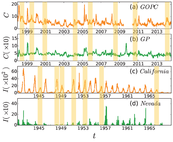
Figure 1: (color online). Time series of recurrent epidemics in two coupled regions or cities. (a) and (b) represent the weekly consultation rates of influenza-like illness (per 1000 consultations) from $1999$ to $2013$ in Hong Kong for the General Out-Patient Clinics (GOPC) and the General Practitioners (GP), respectively, where the data from 2009/6/13 to 2010/5/23 in (a) are not available and the value of $C$ in (b) is from $0$ to $150$. (c) and (d) represent the time series of reported weekly measles infective cases $I$ in California and Nevada, respectively.

The synchronized and mixed outbreak patterns of recurrent epidemics in real data. Monitoring epidemic spreading is vital for us to prevent and control infectious diseases. For this purpose, Hong Kong Department of Health launched a sentinel surveillance system to collect data of infectious diseases, aiming to analyze and predict the trend of infectious spreading in different regions of Hong Kong. In this system, there are about $64$ General Out-Patient Clinics (GOPC) and $50$ General Practitioners (GP), which form two sentinel surveillance networks of Hong Kong www:hongkong , respectively. By these two networks, we can obtain the weekly consultation rates of influenza-like illness (per $1000$ consultations). Fig. 1(a) and (b) show the collected data from $1999$ to $2013$ for the GOPC and GP, respectively, where the data from 2009/6/13 to 2010/5/23 in (a) was not collected by Hong Kong Department of Health and the value of $C$ in (b) is from $0$ to $150$. This weekly consultation rates of influenza-like illness can well reflect the overall influenza-like illness activity in Hong Kong. From the data in Fig. 1(a) and (b) we easily find that there are intermittent peaks, marking the recurrent outbreaks of epidemics. By a second check on the data in Fig. 1(a) and (b) we interestingly find that some peaks occur simultaneously in the two networks at the same time, indicating the appearance of synchronized outbreak pattern. While other peaks appear only in Fig. 1(a) but not in Fig. 1(b), indicating the existence of mixed outbreak pattern (see the light yellow shaded areas).

Is this finding of synchronized and mixed outbreak patterns in recurrent epidemics a specific phenomenon only in Hong Kong? To figure out its generality, we have checked a large number of other recurrent infectious data in different pathogens and in different states and cities in the United States and found the similar phenomenon. Fig. 1(c) and (d) show the data of weekly measles infective cases $I$ in the states of California and Nevada, respectively, which were obtained from the USA National Notifiable Diseases Surveillance System as digitized by Project Tycho measles:2016 ; Scarpino:2016 ; Panhuis:2013 . As California is adjacent to Nevada in west coast of the United States, their climatic conditions are similar. Thus, they can be also considered as two coupled networks. Three more these kinds of examples have been shown in Fig. 1 of SI where the coupled networks are based on states-level influenza data and cities-level measles data, respectively. Therefore, the synchronized and mixed outbreak patterns are general in recurrent epidemics. We will explain their underlying mechanisms in the next subsection.

A two-layered network model of coupled recurrent epidemics. Two classical models of epidemic spreading are the Susceptible-Infected-Susceptible (SIS) model and Susceptible-Infected-Refractory (SIR) model Pastor:2015 . In the SIS model, a susceptible node will be infected by an infected neighbor with rate $\beta$. In the meantime, each infected node will recover with a probability $\gamma$ at each time step. After the transient process, the system reaches a stationary state with a constant infected density $\rho_{I}$. Similarly, in the SIR model, each node can be in one of the three states: Susceptible, Infected, and Refractory. At each time step, a susceptible node will be infected by an infected neighbor with rate $\beta$ and an infected node will become refractory with probability $\gamma$. The infection process will be over when there is no infected $I$. These two models have been widely used in a variety of situations. However, it was pointed out that both the SIS and SIR models are failed to explain the recurrence of epidemics in real data Zheng:2015 ; Stone:2007 .

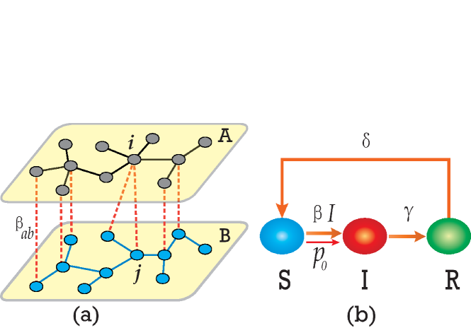
Figure 2: (color online). Schematic figure of the epidemic model to reproduce the synchronized and mixed outbreak patterns. (a) Schematic figure of the two-layered network, where the “black”, “blue” and “red” lines represent the links of the networks $\mathcal{A}$, $\mathcal{B}$ and the inter-network $\mathcal{AB}$, respectively. $\beta_{ab}$ denotes the infectious rate through one interconnection between $\mathcal{A}$ and $\mathcal{B}$. (b) Schematic figure of the extended SIRS model for each node in $\mathcal{A}$ and $\mathcal{B}$, where the symbols $S,I$ and $R$ represent the susceptible, infectious, and refractory states, respectively, and the parameters $\beta,\gamma$ and $\delta$ represent the infectious, refractory and recovery rates, respectively. $p_{0}$ denotes the probability for a susceptible node to be naturally infected by environment or other factors.

To reproduce the synchronized and mixed outbreak patterns, we here present a two-layered network model of coupled recurrent epidemics, shown in Fig. 2 where (a) represents its schematic figure of network topology and (b) denotes the epidemic model at each node. In Fig. 2(a), two networks $\mathcal{A}$ and $\mathcal{B}$ are coupled through some interconnections between them, which form the inter-network $\mathcal{AB}$. For the sake of simplicity, we let the two networks $\mathcal{A}$ and $\mathcal{B}$ have the same size $N_{a}=N_{b}$. We let $\langle k_{a}\rangle$, $\langle k_{b}\rangle$, and $\langle k_{ab}\rangle$ represent the average degrees of the networks $\mathcal{A}$, $\mathcal{B}$ and$\mathcal{AB}$, respectively, see Methods for details. In Fig. 2(b), the epidemic model is adopted from our previous work Zheng:2015 by two steps. In step one, we extend the SIR model to a Susceptible-Infected-Refractory-Susceptible (SIRS) model where a refractory node will become susceptible again with probability $\delta$. In step two, we let each susceptible node have a small probability $p_{0}$ to be infected, which represents the natural infection from environment. Moreover, we let the infectious rate $\beta(t)$ be time dependent, representing its annual and seasonal variations etc. To distinguish the function of the interconnections from that of those links in $\mathcal{A}$ and $\mathcal{B}$, we let $\beta_{ab}$ be the inter-layer infectious rate. In this way, the interaction between $\mathcal{A}$ and $\mathcal{B}$ can be described by the tunable parameter $\beta_{ab}$.

In numerical simulations, we let both the networks $\mathcal{A}$ and $\mathcal{B}$ be the Erdős-Rényi (ER) random networks BA:2002 . To guarantee a recurrent epidemics in each of $\mathcal{A}$ and $\mathcal{B}$, we follow Ref. Zheng:2015 to let $\beta(t)$ be the truncated Gaussian distribution $\mathcal{N}(0.1,0.1^{2})$ and choose $p_{0}=0.01$. Fig. 3(a) and (b) show the evolutions of the infected density $\rho_{I}$ in $\mathcal{A}$ and $\mathcal{B}$, respectively, where the parameters are taken as $\langle k_{a}\rangle=6.5$, $\langle k_{b}\rangle=1.5$, $\langle k_{ab}\rangle=1.0$, and $\beta_{ab}=0.09$. It is easy to observe that some peaks of $\rho_{I}$ appear simultaneously in $\mathcal{A}$ and $\mathcal{B}$, indicating the synchronized outbreak pattern. We also notice that some peaks of $\rho_{I}$ in $\mathcal{A}$ do not have corresponding peaks in $\mathcal{B}$ (see the light yellow shadowed areas in Fig. 3(a) and (b)), indicating the mixed outbreak pattern. Moreover, we do not find the contrary case where there are peaks of $\rho_{I}$ in $\mathcal{B}$ but no corresponding peaks in $\mathcal{A}$, which is also consistent with the empirical observations in Fig. 1(a)-(d).

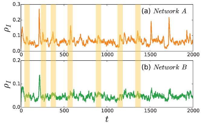
Figure 3: (color online). Reproduced time series of recurrent epidemics in the two-layered network model. (a) and (b) represent the evolutions of the infected density $\rho_{I}$ in the two-layered networks $\mathcal{A}$ and $\mathcal{B}$, respectively, where the parameters are taken as $\langle k_{a}\rangle=6.5$, $\langle k_{b}\rangle=1.5$, $\langle k_{ab}\rangle=1.0$, $\beta(t)\sim\mathcal{N}(0.1,0.1^{2})$, $\beta_{ab}=0.09$, $\gamma=0.2$, $\delta=0.02$, $p_{0}=0.01$, and $N_{a}=N_{b}=1000$.

Mechanism of the synchronized and mixed outbreak patterns. To understand the phenomenon of synchronized and mixed outbreak patterns better, we here study their underlying mechanisms. A key quantity for the phenomenon is the outbreak of epidemic, i.e. the peaks in the time series of Fig. 1. Notice that a peak is usually much higher than its background oscillations. To pick out a peak, we need to define its background/baseline first. As the distributions of both the real data in Fig. 1 and numerical simulations in Fig. 3 are approximately satisfied the normal distribution (see Fig. 2 SI), we define the baseline as $\mu+3\sigma$ with $\mu$ and $\sigma$ being the mean and standard deviation, respectively, which contains about $99.7\%$ data in the normal distribution Patel:1996 . Then, we can count the number of outbreaks in a measured time $t$. Let $n$ be the average number of outbreaks in realizations of the same evolution $t$. Larger $n$ implies more frequent outbreaks. Let $\Delta n=\mid n(\mathcal{A})-n(\mathcal{B})\mid$ be the difference of outbreak numbers between the networks $\mathcal{A}$ and $\mathcal{B}$. Larger $\Delta n$ implies more frequent emergence of the mixed outbreak pattern. In particular, the mixed outbreak pattern will disappear when $\Delta n=0$.

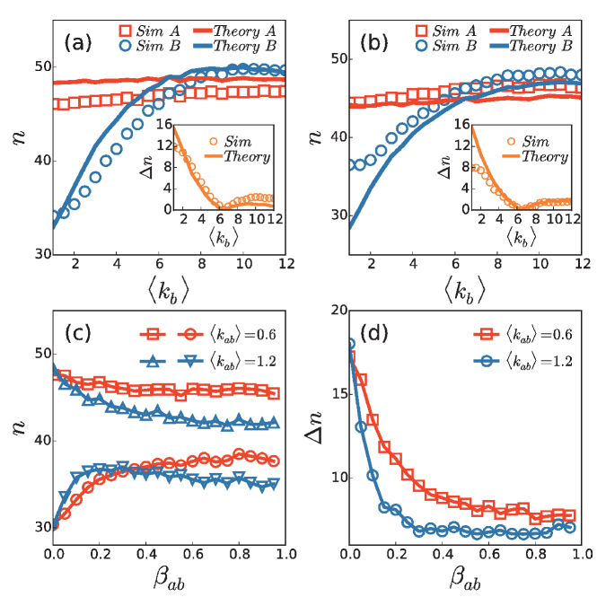
Figure 4: (color online). (a) and (b): Dependence of $n$ on the average degree $\langle k_{b}\rangle$ of network $\mathcal{B}$ for $\beta_{ab}=0.09$ and $0.3$, respectively, where the average degree of network $\mathcal{A}$ is fixed as $\langle k_{a}\rangle=6.5$, $\langle k_{ab}\rangle=1.0$, and the insets show the dependence of $\Delta n=\mid n(\mathcal{A})-n(\mathcal{B})\mid$ on $\langle k_{b}\rangle$. The solid lines represent the theoretical results from Eqs. (A theoretical analysis based on microscopic Markov-chain approach) and (A theoretical analysis based on microscopic Markov-chain approach). (c): Dependence of $n$ on $\beta_{ab}$ with $\langle k_{a}\rangle=6.5$ and $\langle k_{b}\rangle=1.5$ where the “squares” and “circles” represent the case of $\langle k_{ab}\rangle=0.6$ for the networks $\mathcal{A}$ and $\mathcal{B}$, respectively, and the “up triangles” and “down triangles” represent the case of $\langle k_{ab}\rangle=1.2$ for the networks $\mathcal{A}$ and $\mathcal{B}$, respectively. (d): Dependence of $\Delta n$ on $\beta_{ab}$ with $\langle k_{a}\rangle=6.5$ and $\langle k_{b}\rangle=1.5$ where the “squares” and “circles” represent the cases of $\langle k_{ab}\rangle=0.6$ and $1.2$, respectively. The other parameters are set as $\beta(t)\sim\mathcal{N}(0.1,0.1^{2})$, $\gamma=0.2$, $\delta=0.02$, $p_{0}=0.01$, and $N_{a}=N_{b}=1000$. All the results are averaged over $1000$ independent realizations with the simulation steps $t=20000$.

We are interested in how the average degrees and coupling influence the numbers $n$ and $\Delta n$. Figure 4(a) and (b) show the dependence of $n$ on the average degree $\langle k_{b}\rangle$ of network $\mathcal{B}$ for $\beta_{ab}=0.09$ and $0.3$, respectively, where the average degree of network $\mathcal{A}$ is fixed as $\langle k_{a}\rangle=6.5$. It is easy to see from Fig. 4(a) and (b) that the number $n(\mathcal{B})$ of network $\mathcal{B}$ will gradually increase with the increase of $\langle k_{b}\rangle$, while the number $n(\mathcal{A})$ of network $\mathcal{A}$ keeps approximately constant, indicating that a larger $\langle k_{b}\rangle$ is in favor of the recurrent outbreaks. Specifically, $n(\mathcal{B})$ will reach $n(\mathcal{A})$ when $\langle k_{b}\rangle$ is increased to the value of $\langle k_{b}\rangle=\langle k_{a}\rangle=6.5$, see the insets in Fig. 4(a) and (b) for the minimum of $\Delta n$. For details, Fig. 3 in SI shows the evolution of infected densities $\rho_{I}$ for the cases of $\langle k_{a}\rangle=\langle k_{b}\rangle$, confirming the result of $\Delta n=0$ in Fig. 4(a) and (b). On the other hand, comparing the two insets in Fig. 4 (a) and (b), we find that $\Delta n$ in Fig. 4(a) is greater than the corresponding one in Fig. 4(b), indicating that a larger $\beta_{ab}$ is in favor of suppressing the mixed outbreak pattern. These results can be also theoretically explained by the microscopic Markov-chain approach, see Methods for details. The solid lines in Fig. 4 (a) and (b) represent the theoretical results from Eqs. (A theoretical analysis based on microscopic Markov-chain approach) and (A theoretical analysis based on microscopic Markov-chain approach). It is easy to see that the theoretical results are consistent with the numerical simulations very well.

Fig. 4(c) and (d) show the influences of the coupling parameters such as $\beta_{ab}$ and $k_{ab}$ for the outbreak number $n$ and the difference of outbreak number $\Delta n$, respectively, where $\langle k_{a}\rangle=6.5$ and $\langle k_{b}\rangle=1.5$. From Fig. 4(c) we see that for the case of $k_{ab}=0.6$, $n(\mathcal{A})$ is an approximate constant and $n(\mathcal{B})$ gradually increase with $\beta_{ab}$. While for the case of $k_{ab}=1.2$, both $n(\mathcal{A})$ and $n(\mathcal{B})$ change with $\beta_{ab}$, indicating that both $k_{ab}$ and $\beta_{ab}$ take important roles in the synchronized and mixed outbreak patterns. From Fig. 4(d) we see that the case of $k_{ab}=1.2$ decreases faster than the case of $k_{ab}=0.6$, indicating that both the larger $k_{ab}$ and larger $\beta_{ab}$ are in favor of the synchronized outbreak pattern. That is, the stronger coupling will suppress the mixed outbreak pattern but enhance the synchronized outbreak pattern. On the contrary, the weaker coupling is in favor of the mixed epidemic outbreak pattern but suppress the synchronized outbreak pattern. For details, Fig. 4 in SI shows the evolution of infected densities $\rho_{I}$ for different $\beta_{ab}$, confirming the above results.

Coupling induced correlation between the epidemics of the two networks. The coupling between the two layers is represented by the pair of variables $(\beta_{ab},\langle k_{ab}\rangle)$. Qualitatively, larger $\beta_{ab}$ and $\langle k_{ab}\rangle$ represent stronger coupling. To quantitatively represent the effects of $\beta_{ab}$ and $\langle k_{ab}\rangle$, we here measure the cross-correlation, $r$, defined in Eq. (19), which can show some information beyond the synchronized and mixed outbreak patterns. By Eq. (19) we first calculate the coefficient $r$ between the two time series of GOPC and GP and find $r=0.66$, indicating that these two data are highly correlated. Fig. 5(a) shows the correspondence between the two time series of GOPC and GP. Then, we check the influence of coupling on the coefficient $r$. Fig. 5(b) shows the dependence of $r$ on $\beta_{ab}$ for $\langle k_{ab}\rangle=0.2,0.5,1.0$ and $2.0$, respectively. We see that $r$ increases with $\beta_{ab}$ for a fixed $\langle k_{ab}\rangle$ and also increases with $\langle k_{ab}\rangle$ for a fixed $\beta_{ab}$, indicating the enhanced correlation by the coupling strength. Very interesting, we find that for the case of $\langle k_{ab}\rangle=1.0$ in Fig. 5(b), the point of $r=0.66$ corresponds to $\langle\beta_{ab}\rangle=0.09$ (see the purple “star”), implying that the coupling in Fig. 5(a) is equivalent to the case of $\langle k_{ab}\rangle=1.0$ and $\langle\beta_{ab}\rangle=0.09$ in Fig. 5(b). In this sense, we may draw a horizontal line passing the purple “star” in Fig. 5(b) (see the dashed line) and its crossing points with all the curves there will also represent the equivalent coupling in Fig. 5(a). However, we notice that the horizontal line has no crossing point with the curve of $\langle k_{ab}\rangle=0.2$, indicating that there is a threshold of $\langle k_{ab}\rangle$ for the appearance of $r=0.66$ in Fig. 5(a).

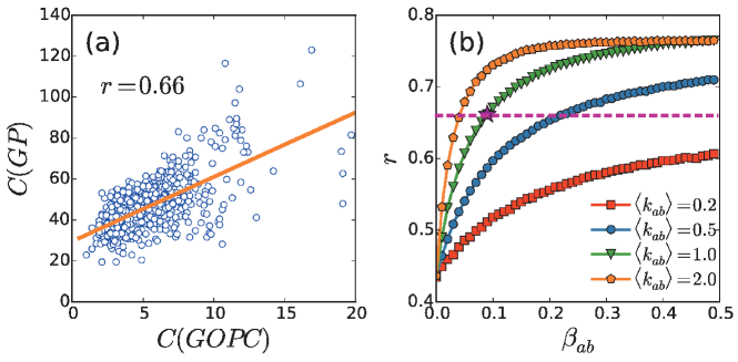
Figure 5: (color online.) Correlation between the two coupled layers. (a) Correlation between the two time series of GOPC and GP. (b) Dependence of the correlation coefficient $r$ on $\beta_{ab}$ for $\langle k_{ab}\rangle=0.2,0.5,1.0$ and $2.0$, respectively, where the purple “star” and its related dashed line represent the point of $r=0.66$. Other parameters are the same as in Fig. 3(a) and (b).

It is maybe helpful to understand the influence of $(\beta_{ab},\langle k_{ab}\rangle)$ on epidemics from the aspect of purely coupling in network structure. We know that a critical problem in coupled networks is when they behave as separate networks vs when they behave as a solid single network Radicchi:2013 ; Sahneh:2015 . In our case here, the synchrony of epidemic in the two layers corresponds the case of strong coupling while the mixed pattern represents the case of weak coupling. Therefore, the synchrony and mixed patterns also reflect the influence of network structure on its dynamics. On the other hand, we notice from Fig. 5(b) that there is a finite value of $r\approx 0.43$ when $\beta_{ab}=0$, implying that the same infection probability $\beta(t)$ in the two networks do have a contribution to the correlation $r$. However, the further increase of $r$ in Fig. 5(b) reflects the influence from the coupling parameters of $(\beta_{ab},\langle k_{ab}\rangle)$. From Fig. 5(b) we see that for a fixed $\beta_{ab}$, $r$ increases with $\langle k_{ab}\rangle$, indicating the influence of $\langle k_{ab}\rangle$. While for a fixed $\langle k_{ab}\rangle$, $r$ increases with $\beta_{ab}$, indicating the influence of $\beta_{ab}$. Therefore, the further increase of correlation from $r\approx 0.43$ do come from the coupling between the two time series.

Discussion

The dependence of the synchronized and mixed outbreak patterns on the average degrees of networks $\mathcal{A}$ and $\mathcal{B}$ may be also understood from the aspect of their epidemic thresholds. By the theoretical analysis in Methods we obtain the epidemic thresholds as $\beta_{c}^{A}=\frac{\gamma}{\langle k_{a}\rangle}$ and $\beta_{c}^{B}=\frac{\gamma}{\langle k_{b}\rangle}$ in Eq. (18), when the two networks are weakly coupled. For the case of $\langle k_{a}\rangle>\langle k_{b}\rangle$, we have $\beta_{c}^{A}<\beta_{c}^{B}$. When $\beta$ satisfies $\beta<\beta_{c}^{A}<\beta_{c}^{B}$, the epidemics cannot survive in each of networks $\mathcal{A}$ and $\mathcal{B}$. Thus, the infected fraction will be approximately zero, i.e. no epidemic outbreak in both $\mathcal{A}$ and $\mathcal{B}$. It should be noticed that this result just holds for the case of weakly coupling. When coupling is strong, it is possible for epidemic to occur in the coupled network even when $\beta$ is below the epidemic threshold of each layer Sahneh:2013 . When $\beta$ satisfies $\beta>\beta_{c}^{B}>\beta_{c}^{A}$, the epidemics will survive in both networks $\mathcal{A}$ and $\mathcal{B}$, indicating an outbreak will definitely occur in both of them. These two cases are trivial. However, when $\beta$ is in between $\beta_{c}^{A}$ and $\beta_{c}^{B}$, some interesting results may be induced by coupling. When coupling is weak, it is possible for epidemic to outbreak only in network $\mathcal{A}$ but not in network $\mathcal{B}$. When coupling is increased slightly, it will be also possible for epidemic to outbreak sometimes in network $\mathcal{B}$, i.e. resulting a mixed outbreak pattern. Once coupling is further increased to large enough, a synchronized outbreak pattern will be resulted.

So far, the reported results are from the ER random networks $\mathcal{A}$ and $\mathcal{B}$. We are wondering whether it is possible to still observe the phenomenon of the synchronized and mixed outbreak patterns in other network topologies. For this purpose, we here take the scale-free network BA:2002 as an example. Very interesting, by repeating the above simulation process in scale-free networks we have found the similar phenomenon as in ER random networks, see Figs. 5-7 in SI for details. Therefore, the synchronized and mixed outbreak patterns are a general phenomena in multi-layered epidemic networks.

In sum, the epidemic spreading has been well studied in the past decades, mainly focused on both the single and multi-layered networks. However, only a few works focused on the aspect of recurrent epidemics, including both the models in homogeneous population Stone:2007 and our recent model in a single network Zheng:2015 . We here report from the real data that the epidemics from different networks are in fact not isolated but correlated, implying that they should be considered as a multi-layered network. Motivated by this discovery, we present a two-layered network model to reproduce the correlated recurrent epidemics in coupled networks. More importantly, we find that this model can reproduce both the synchronized and mixed outbreak patterns in real data. The two-layered network favors to show the synchronized pattern when the average degrees of the two coupled networks have a large difference and shows the mixed pattern when their average degrees are very close. Besides the degree difference between the two networks, the coupling strength between the two layers has also significant influence to the synchronized and mixed outbreak patterns. We show that both the larger $\beta_{ab}$ and larger $\langle k_{ab}\rangle$ are in favor of the synchronized pattern but suppress the mixed pattern. This finding thus shows a new way to understand the epidemics in realistic multi-layered networks. Its further studies and potential applications in controlling the recurrent epidemics may be an interesting topic in near future.

Methods

A two-layered network model of recurrent epidemic spreading

We consider a two-layered network model with coupling between its two layers, i.e. the networks $\mathcal{A}$ and $\mathcal{B}$ in Fig. 2(a). We let the two networks have the same size $N_{a}=N_{b}=N$ and their degree distributions $P_{A}(k)$ and $P_{B}(k)$ be different. We may imagine the network $\mathcal{A}$ as a human contact network for one geographic region and the network $\mathcal{B}$ for a separated region. Each node in the two-layered network has two kinds of links, i.e. intra-links within $\mathcal{A}$ or $\mathcal{B}$ and the interconnection between $\mathcal{A}$ and $\mathcal{B}$. The former consists of the degree distributions $P_{A}(k)$ and $P_{B}(k)$ while the latter the interconnection network. We let $\langle k_{a}\rangle$, $\langle k_{b}\rangle$, and $\langle k_{ab}\rangle$ represent the average degrees of networks $\mathcal{A}$, $\mathcal{B}$ and interconnection network $\mathcal{AB}$, respectively. In details, we firstly generate two separated networks $\mathcal{A}$ and $\mathcal{B}$ with the same size $N$ and different degree distributions $P_{A}(k)$ and $P_{B}(k)$, respectively. Then, we add links between $\mathcal{A}$ and $\mathcal{B}$. That is, we randomly choose two nodes from $\mathcal{A}$ and $\mathcal{B}$ and then connect them if they are not connected yet. Repeat this process until the steps we planned. In this way, we obtain an uncorrelated two-layered network.

To discuss epidemic spreading in the two-layered network, we use the extended SIRS model, see Fig. 2(b) for its schematic illustration. In this model, a susceptible node has three ways to be infected. The first one is the natural infection from environment or unknown reasons, represented by a small probability $p_{0}$. The second one is the infection from contacting with infected individuals in the network $\mathcal{A}$ (or $\mathcal{B}$), represented by $\beta(t)$. And the third one is the infection from another network, represented by $\beta_{ab}$ (see Fig. 2(a)). Thus, a susceptible node will become infected with a probability $1-(1-p_{0})(1-\beta(t))^{k^{inf}}(1-\beta_{ab})^{k_{ab}^{inf}}$ where $k^{inf}$ is the infected neighbors in the same network and $k_{ab}^{inf}$ is the infected neighbors in another network. At the same time, an infected node will become refractory by a probability $\gamma$ and a refractory node will become susceptible again by a probability $\delta$.

In numerical simulations, the dependence of $\beta(t)$ on time is implemented as follows Zheng:2015 : we divide the total time $t$ into multiple segments with length $T$ and let $T=52$, corresponding to the $52$ weeks in one year. We let $\beta(t)$ be a constant in each segment, which is randomly chosen from the truncated Gaussian distribution $\mathcal{N}(0.1,0.1^{2})$. Once a $\beta(t)<0$ or $\beta(t)>1$ is chosen, we discard it and then choose a new one. At the same time, we fix $\gamma=0.2$ and $\delta=0.02$ and set $\beta_{ab}$ as the tunable parameter.

A theoretical analysis based on microscopic Markov-chain approach

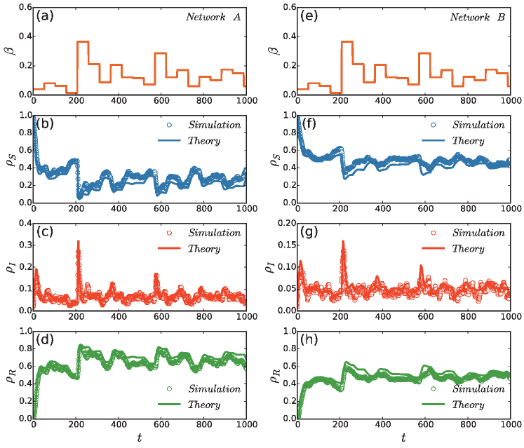
Figure 6: (color online.) Comparison between the theoretical solutions and numerical simulations. The left and right panels are for the networks $\mathcal{A}$ and $\mathcal{B}$, respectively. All the parameters are the same as in Fig. 3(a) and (b). (a) and (e) $\beta(t)$ versus $t$; (b) and (f) $\rho_{S}$ versus $t$; (c) and (g) $\rho_{I}$ versus $t$; (d) and (h) $\rho_{R}$ versus $t$. In (b)-(d) and (f)-(h), the solid curves represent the theoretical solutions while the “circles” represent the numerical simulations.

Let $P^{S}_{i,A}(t)$, $P^{I}_{i,A}(t)$, $P^{R}_{i,A}(t)$ be the probabilities for node $i$ in network $\mathcal{A}$ to be in one of the three states of $S,I$ and $R$ at time $t$, respectively. Similarly, we have $P^{S}_{i,B}(t)$, $P^{I}_{i,B}(t)$ and $P^{R}_{i,B}(t)$ in network $\mathcal{B}$. They satisfy the conservation law

$$P^{S}_{i,A}(t)+P^{I}_{i,A}(t)+P^{R}_{i,A}(t)=1,\quad P^{S}_{i,B}(t)+P^{I}_{i,B}(t)+P^{R}_{i,B}(t)=1.$$ (1)

According to the Markov-chain approach Gomez:2010 ; Gomez:2011 ; Granell:2013 ; Zheng:2015 ; Valdano:2015 , we introduce

$$\rho^{A}_{S}(t)=\frac{1}{N}\sum\limits_{i=1}^{N}P^{S}_{i,A}(t),\quad\rho^{A}_{I}(t)=\frac{1}{N}\sum\limits_{i=1}^{N}P^{I}_{i,A}(t),\quad\rho^{A}_{R}(t)=\frac{1}{N}\sum\limits_{i=1}^{N}P^{R}_{i,A}(t),$$

$$\rho^{B}_{S}(t)=\frac{1}{N}\sum\limits_{i=1}^{N}P^{S}_{i,B}(t),\quad\rho^{B}_{I}(t)=\frac{1}{N}\sum\limits_{i=1}^{N}P^{I}_{i,B}(t),\quad\rho^{B}_{R}(t)=\frac{1}{N}\sum\limits_{i=1}^{N}P^{R}_{i,B}(t),$$

where $\rho^{A}_{S}(t)$, $\rho^{A}_{I}(t)$ and $\rho^{A}_{R}(t)$ represent the densities of susceptible, infected, and refractory individuals at time $t$ in network $\mathcal{A}$, respectively. Similarly, we have $\rho^{B}_{S}(t)$, $\rho^{B}_{I}(t)$ and $\rho^{B}_{R}(t)$ in network $\mathcal{B}$.

Let $q^{S,I}_{i,A}(t)$, $q^{I,R}_{i,A}(t)$ and $q^{R,S}_{i,A}(t)$ be the transition probabilities from the state $S$ to $I$, $I$ to $R$, and $R$ to $S$ in network $\mathcal{A}$, respectively. By the Markov chain approach Gomez:2010 ; Valdano:2015 we have

$$q^{S,I}_{i,A}(t) = 1-(1-p_{0})\prod_{l\in\Lambda_{i,A}}(1-\beta(t)P^{I}_{l,A}(t))\prod_{v\in\Lambda_{i,B}}(1-\beta_{ab}P^{I}_{v,B}(t)),$$

$$q^{I,R}_{i,A}(t) = \gamma,$$ (2)

$$q^{R,S}_{i,A}(t) = \delta,$$

where $\Lambda_{i,A}$ represents the neighboring set of node $i$ in network $\mathcal{A}$. The term $(1-p_{0})$ in Eq. (A theoretical analysis based on microscopic Markov-chain approach) represents the probability that node $i$ is not infected by the environment. The term $\prod_{l\in\Lambda_{i,A}}(1-\beta(t)P^{I}_{l,A}(t))$ is the probability that node $i$ is not infected by the infected neighbors in network $\mathcal{A}$. While the term $\prod_{v\in\Lambda_{i,B}}(1-\beta_{ab}P^{I}_{v,B}(t))$ is the probability that node $i$ is not infected by the infected neighbors in another network. Thus, $(1-p_{0})\prod_{l\in\Lambda_{i,A}}(1-\beta(t)P^{I}_{l,A}(t))\prod_{v\in\Lambda_{i,B}}(1-\beta_{ab}P^{I}_{v,B}(t))$ is the probability for node $i$ to be in the susceptible state. Similarly, for the node in network $\mathcal{B}$, we have

$$q^{S,I}_{i,B}(t) = 1-(1-p_{0})\prod_{l\in\Lambda_{i,B}}(1-\beta(t)P^{I}_{l,B}(t))\prod_{v\in\Lambda_{i,A}}(1-\beta_{ab}P^{I}_{v,A}(t)),$$

$$q^{I,R}_{i,B}(t) = \gamma,$$ (3)

$$q^{R,S}_{i,B}(t) = \delta.$$

Based on these analysis, we formulate the following difference equations

$$P^{S}_{i,A}(t+1) = P^{S}_{i,A}(t)(1-q^{S,I}_{i,A}(t))+P^{R}_{i,A}(t)q^{R,S}_{i,A}(t),$$

$$P^{I}_{i,A}(t+1) = P^{I}_{i,A}(t)(1-q^{I,R}_{i,A}(t))+P^{S}_{i,A}(t)q^{S,I}_{i,A}(t),$$ (4)

$$P^{R}_{i,A}(t+1) = P^{R}_{i,A}(t)(1-q^{R,S}_{i,A}(t))+P^{I}_{i,A}(t)q^{I,R}_{i,A}(t).$$

$$P^{S}_{i,B}(t+1) = P^{S}_{i,B}(t)(1-q^{S,I}_{i,B}(t))+P^{R}_{i,B}(t)q^{R,S}_{i,B}(t),$$

$$P^{I}_{i,B}(t+1) = P^{I}_{i,B}(t)(1-q^{I,R}_{i,B}(t))+P^{S}_{i,B}(t)q^{S,I}_{i,B}(t),$$ (5)

$$P^{R}_{i,B}(t+1) = P^{R}_{i,B}(t)(1-q^{R,S}_{i,B}(t))+P^{I}_{i,B}(t)q^{I,R}_{i,B}(t).$$

The first term on the right-hand side of the first equation of Eq. (A theoretical analysis based on microscopic Markov-chain approach) is the probability that node $i$ is remained as susceptible state. The second term stands for the probability that node $i$ is changed from refractory to susceptible state. Similarly, we have the same explanation for the other equations of Eqs. (A theoretical analysis based on microscopic Markov-chain approach) and (A theoretical analysis based on microscopic Markov-chain approach). Substituting Eqs. (A theoretical analysis based on microscopic Markov-chain approach) and (A theoretical analysis based on microscopic Markov-chain approach) into Eqs. (A theoretical analysis based on microscopic Markov-chain approach) and (A theoretical analysis based on microscopic Markov-chain approach), we obtain the microscopic Markov dynamics as follows

$$P^{S}_{i,A}(t+1) = P^{S}_{i,A}(t)[(1-p_{0})\prod_{l\in\Lambda_{i,A}}(1-\beta(t)P^{I}_{l,A}(t))\prod_{v\in\Lambda_{i,B}}(1-\beta_{ab}P^{I}_{v,B}(t))]+P^{R}_{i,A}(t)\delta,$$

$$P^{I}_{i,A}(t+1) = P^{I}_{i,A}(t)(1-\gamma)+P^{S}_{i,A}(t)[1-(1-p_{0})\prod_{l\in\Lambda_{i,A}}(1-\beta(t)P^{I}_{l,A}(t))\prod_{v\in\Lambda_{i,B}}(1-\beta_{ab}P^{I}_{v,B}(t))],$$ (6)

$$P^{R}_{i,A}(t+1) = P^{R}_{i,A}(t)(1-\delta)+P^{I}_{i,A}(t)\gamma.$$

$$P^{S}_{i,B}(t+1) = P^{S}_{i,B}(t)[(1-p_{0})\prod_{l\in\Lambda_{i,B}}(1-\beta(t)P^{I}_{l,B}(t))\prod_{v\in\Lambda_{i,A}}(1-\beta_{ab}P^{I}_{v,A}(t))]+P^{R}_{i,B}(t)\delta,$$

$$P^{I}_{i,B}(t+1) = P^{I}_{i,B}(t)(1-\gamma)+P^{S}_{i,B}(t)[1-(1-p_{0})\prod_{l\in\Lambda_{i,B}}(1-\beta(t)P^{I}_{l,B}(t))\prod_{v\in\Lambda_{i,A}}(1-\beta_{ab}P^{I}_{v,A}(t))],$$ (7)

$$P^{R}_{i,B}(t+1) = P^{R}_{i,B}(t)(1-\delta)+P^{I}_{i,B}(t)\gamma.$$

Instead of getting the analytic solutions of Eqs. (A theoretical analysis based on microscopic Markov-chain approach) and (A theoretical analysis based on microscopic Markov-chain approach), we solve them by numerical integration. We set the initial conditions as $P^{S}_{i,A}(0)=1.0$, $P^{I}_{i,A}(0)=0.0$, $P^{R}_{i,A}(0)=0.0$, $P^{S}_{i,B}(0)=1.0$, $P^{I}_{i,B}(0)=0.0$, and $P^{R}_{i,B}(0)=0.0$. To conveniently compare the solutions with the numerical simulations in the section Results, we use the same set of $\beta(t)$ for both the integration and numerical simulations. Fig. 6 shows the results where the left and right panels are for the networks $\mathcal{A}$ and $\mathcal{B}$, respectively. In Fig. 6(b)-(d) and Fig. 6(f)-(h), the solid curves represent the theoretical solutions while the “circles” represent the numerical simulations. It is easy to see that the theoretical solutions are consistent with the numerical simulations very well.

A theoretical analysis based on mean field theory

To go deeper into the mechanism of the synchronized and mixed outbreak patterns, we try another theoretical analysis on mean field equations. Let $s^{A}(t)$, $i^{A}(t)$ and $r^{A}(t)$ represent the densities of susceptible, infected, and refractory individuals at time $t$ in network $\mathcal{A}$, respectively. Similarly, we have $s^{B}(t)$, $i^{B}(t)$ and $r^{B}(t)$ in network $\mathcal{B}$. Then, they satisfy

$$s^{A}(t)+i^{A}(t)+r^{A}(t)=1,\quad s^{B}(t)+i^{B}(t)+r^{B}(t)=1.$$ (8)

According to the mean-field theory, we have the following ordinary differential equations

$$\frac{ds^{A}(t)}{dt} = -p_{0}s^{A}(t)-\beta(t)\langle k_{a}\rangle s^{A}(t)i^{A}(t)-\beta_{ab}\langle k_{ab}\rangle s^{A}(t)i^{B}(t)+\delta r^{A}(t),$$ (9)

$$\frac{di^{A}(t)}{dt} = p_{0}s^{A}(t)+\beta(t)\langle k_{a}\rangle s^{A}(t)i^{A}(t)+\beta_{ab}\langle k_{ab}\rangle s^{A}(t)i^{B}(t)-\gamma i^{A}(t),$$ (10)

$$\frac{dr^{A}(t)}{dt} = \gamma i^{A}(t)-\delta r^{A}(t),$$ (11)

$$\frac{ds^{B}(t)}{dt} = -p_{0}s^{B}(t)-\beta(t)\langle k_{b}\rangle s^{B}(t)i^{B}(t)-\beta_{ab}\langle k_{ab}\rangle s^{B}(t)i^{A}(t)+\delta r^{B}(t),$$ (12)

$$\frac{di^{B}(t)}{dt} = p_{0}s^{B}(t)+\beta(t)\langle k_{b}\rangle s^{B}(t)i^{B}(t)+\beta_{ab}\langle k_{ab}\rangle s^{B}(t)i^{A}(t)-\gamma i^{B}(t),$$ (13)

$$\frac{dr^{B}(t)}{dt} = \gamma i^{B}(t)-\delta r^{B}(t).$$ (14)

Specifically, we consider a case of single epidemic outbreak with extremely weak coupling, i.e. $p_{0}=0$ and $\beta_{ab}\approx 0$. In the steady state, we have

$$\frac{ds^{A}(t)}{dt}=0,\quad\frac{di^{A}(t)}{dt}=0,\quad\frac{ds^{B}(t)}{dt}=0,\quad\frac{di^{B}(t)}{dt}=0,$$ (15)

which gives

$$s^{A}(t)=\frac{\gamma}{\beta(t)\langle k_{a}\rangle},\quad r^{A}(t)=\frac{\gamma}{\delta}i^{A}(t),\quad s^{B}(t)=\frac{\gamma}{\beta(t)\langle k_{b}\rangle},\quad r^{B}(t)=\frac{\gamma}{\delta}i^{B}(t).$$ (16)

Substituting Eq. (16) into Eq. (8) we obtain

$$\frac{\gamma}{\beta(t)\langle k_{a}\rangle}+(\frac{\gamma}{\delta}+1)i^{A}(t)=1,\quad\frac{\gamma}{\beta(t)\langle k_{b}\rangle}+(\frac{\gamma}{\delta}+1)i^{B}(t)=1.$$ (17)

The critical point can be given by letting $i^{A}(t)$ and $i^{B}(t)$ in Eq. (17) change from zero to nonzero, which gives

$$\beta_{c}^{A}=\frac{\gamma}{\langle k_{a}\rangle},\quad\beta_{c}^{B}=\frac{\gamma}{\langle k_{b}\rangle}.$$ (18)

For the considered networks with $\langle k_{a}\rangle>\langle k_{b}\rangle$, we have $\beta_{c}^{A}<\beta_{c}^{B}$.

Cross-correlation measure

In statistics, the Pearson correlation coefficient is a measure of the linear correlation between two variables. If two time series $\{X_{t}\}$ and $\{Y_{t}\}$ have the mean values $\overline{X}$ and $\overline{Y}$, we can define the correlation coefficient $r$ as follows

$$r=\frac{\sum\limits_{t=1}^{n}(X_{t}-\overline{X})(Y_{t}-\overline{Y})}{\sqrt{\sum\limits_{t=1}^{n}(X_{t}-\overline{X})^{2}\cdot\sum\limits_{t=1}^{n}(Y_{t}-\overline{Y})^{2}}}$$ (19)

To analyze the correlations of the growth trends between the two time series, we investigates their cross-correlation $r(t)$ in a given window $w_{t}$ Podobnik:2008 ; Wang:2016 , i.e. $\{X_{t},\ X_{t+1},\ \ldots,X_{t+w_{t}}\}$ and $\{Y_{t},\ Y_{t+1},\ \ldots,Y_{t+w_{t}}\}$. $\{X_{t}\}$ and $\{Y_{t}\}$ will share the same trend in the time interval $w_{t}$ when $r(t)>0$ and the opposite growth trend when $r(t)<0$. In this work, we let the whole time series be one window, i.e. with $w_{t}$ being the total evolutionary time $t$.

Author contributions

M.Z. and Z.L. conceived the research project. M.Z., M.Z., B.M. and Z.L. performed research and analyzed the results. M.Z., B.M. and Z.L. wrote the paper. All authors reviewed and approved the manuscript.

Additional information

Competing financial interests: The authors declare no competing financial interests. Correspondence and requests for materials should be addressed to Z.L. (zhliu@phy.ecnu.edu.cn).

References

- (1) Pastor-Satorras, R., & Vespignani, A., Epidemic spreading in scale-free networks. Phys. Rev. Lett. 86, 3200 (2001).
- (2) Boguñá, M., & Pastor-Satorras, R., Epidemic spreading in correlated complex networks. Phys. Rev. E 66, 047104 (2002).
- (3) Ferreira, S. C., Castellano, C., & Pastor-Satorras, R., Epidemic thresholds of the susceptible-infected-susceptible model on networks: A comparison of numerical and theoretical results. Phys. Rev. E 86, 041125 (2012).
- (4) Boguñá, M., Castellano, C., & Pastor-Satorras, R., Nature of the epidemic threshold for the susceptible-infected-susceptible dynamics in networks. Phys. Rev. Lett. 111, 068701 (2013).
- (5) Parshani, R., Carmi, S., & Havlin, S., Epidemic threshold for the susceptible-infectious-susceptible model on random networks. Phys. Rev. Lett. 104, 258701 (2010).
- (6) Castellano, C., & Pastor-Satorras, R., Thresholds for epidemic spreading in networks. Phys. Rev. Lett. 105, 218701 (2010).
- (7) Colizza, V., Pastor-Satorras, R., & Vespignani, A., Reaction-diffusion processes and metapopulation models in heterogeneous networks. Nature Phys. 3, 276-282 (2007).
- (8) Colizza, V., & Vespignani, A., Invasion threshold in heterogeneous metapopulation networks. Phys. Rev. Lett. 99, 148701 (2007).
- (9) Baronchelli, A., Catanzaro, M., & Pastor-Satorras, R., Bosonic reaction-diffusion processes on scale-free networks. Phys. Rev. E 78, 016111 (2008).
- (10) Tang, M., Liu, L., & Liu, Z., Influence of dynamical condensation on epidemic spreading in scale-free networks. Phys. Rev. E 79, 016108 (2009).
- (11) Vazquez, A., Racz, B., Lukacs, A., & Barabasi, A. L., Impact of non-Poissonian activity patterns on spreading processes. Phys. Rev. Lett. 98, 158702 (2007).
- (12) Meloni, S., Arenas, A., & Moreno, Y., Traffic-driven epidemic spreading in finite-size scale-free networks. Proc. Natl. Acad. Sci. USA 106, 16897-16902 (2009).
- (13) Balcan, D., Colizza, V., Gonçalves, B., Hu, H., Ramasco, J. J., & Vespignani, A., Multiscale mobility networks and the spatial spreading of infectious diseases. Proc. Natl. Acad. Sci. USA 106, 21484-21489 (2009).
- (14) Ruan, Z., Tang, M., & Liu, Z., Epidemic spreading with information-driven vaccination. Phys. Rev. E 86, 036117 (2012).
- (15) Liu, S., Perra, N., Karsai, M., & Vespignani, A., Controlling contagion processes in activity driven networks. Phys. Rev. Lett. 112, 118702 (2014).
- (16) Tang, M., Liu, Z., & Li, B., Epidemic spreading by objective traveling. Europhys. Lett. 87, 18005 (2009).
- (17) Liu, Z., Effect of mobility in partially occupied complex networks. Phys. Rev. E 81, 016110 (2010).
- (18) Pastor-Satorras, R., Castellano, C., Van Mieghem, P., & Vespignani, A., Epidemic processes in complex networks. Reviews of modern physics, 87(3), 925 (2015).
- (19) A. Barrat, M. Barthelemy, & A. Vespignani, Dynamical Processes on Complex Networks. (Cambridge University Press, Cambridge, England, 2008).
- (20) Dorogovtsev, S. N., Goltsev, A. V., & Mendes, J. F., Critical phenomena in complex networks. Rev. Mod. Phys. 80, 1275 (2008).
- (21) Boccaletti, S., Bianconi, G., Criado, R., del Genio, C. I., Gómez-Gardeñes, J., Romance, M., Sendiña-Nadal, I., Wang, Z., & Zanin, M., The structure and dynamics of multilayer networks. Phys. Rep. 544, 1 (2014).
- (22) Kivelä, M., Arenas, A., Barthelemy, M., Gleeson, J. P., Moreno, Y. & Porter, M. A., Multilayer networks. J. Complex Netw. 2, 203 (2014).
- (23) Feng, L., Monterola, C. P., & Hu, Y., The simplified self-consistent probabilities method for percolation and its application to interdependent networks. New Journal of Physics, 17(6), 063025 (2015).
- (24) Sahneh, F. D., Scoglio, C., & Chowdhury, F. N., Effect of coupling on the epidemic threshold in interconnected complex networks: A spectral analysis. In 2013 American Control Conference (pp. 2307-2312). IEEE (2013).
- (25) Wang, H., Li, Q., D’Agostino, G., Havlin, S., Stanley, H. E., & Van Mieghem, P. Effect of the interconnected network structure on the epidemic threshold. Phys. Rev. E 88(2) 022801 (2013).
- (26) Yagan, O., Qian, D., Zhang, J., & Cochran, D. Conjoining speeds up information diffusion in overlaying social-physical networks. IEEE J. Sel. Areas Commun. 31(6), 1038-1048 (2013).
- (27) Newman, M. E. Threshold effects for two pathogens spreading on a network. Phys. Rev. Lett. 95(10) 108701 (2005).
- (28) Marceau, V., Noël, P. A., Hébert-Dufresne, L., Allard, A., & Dubé, L. J., Modeling the dynamical interaction between epidemics on overlay networks. Phys. Rev. E 84 026105 (2011).
- (29) Zhao, Y., Zheng, M., & Liu, Z., A unified framework of mutual influence between two pathogens in multiplex networks. Chaos 24, 043129 (2014).
- (30) Buono, C., & Braunstein, L. A., Immunization strategy for epidemic spreading on multilayer networks. Europhy. Lett. 109(2), 26001 (2015).
- (31) Buono, C., Alvarez-Zuzek, L. G., Macri, P. A., & Braunstein, L. A., Epidemics in partially overlapped multiplex networks. PloS one, 9(3), e92200 (2014).
- (32) Little, R. G., Controlling cascading failure: Understanding the vulnerabilities of interconnected infrastructures. J. Urban Technology 9, 109-123 (2002).
- (33) Rosato, V., Issacharoff, L., Tiriticco, F., Meloni, S., Porcellinis, S., & Setola, R., Modelling interdependent infrastructures using interacting dynamical models. J. Critical Infrast. 4 63 (2008).
- (34) Buldyrev, S. V., Parshani, R., Paul, G., Stanley, H. E., & Havlin, S., Catastrophic cascade of failures in interdependent networks. Nature 464, 1025 (2010).
- (35) De Domenico, M., Solé-Ribalta, A., Gómez, S., & Arenas, A., Navigability of interconnected networks under random failures. Proc. Natl. Acad. Sci. USA 111, 8351 (2014).
- (36) Parshani, R., Rozenblat, C., Ietri, D., Ducruet, C., & Havlin, S., Inter-similarity between coupled networks. Europhy. Lett. 92, 68002 (2010).
- (37) Reis, S. D., Hu, Y., Babino, A., Andrade Jr, J. S., Canals, S., Sigman, M., & Makse, H. A., Avoiding catastrophic failure in correlated networks of networks. Nat. Phys. 10, 762 (2014).
- (38) Vidal, M., Cusick, M. E., & Barabási, A. L., Interactome networks and human disease. Cell 144, 986 (2011).
- (39) White, J. G., Southgate, E., Thomson, J. N., & Brenner, S., The structure of the nervous system of the nematode Caenorhabditis elegans. Phil. Trans. Royal Soc. London B, 314, 1 (1986).
- (40) Min, B., Gwak, S. H., Lee, N., & Goh, K. I., Layer-switching cost and optimality in information spreading on multiplex networks. Sci. Rep. 6, 21392 (2016).
- (41) Dickison, M., Havlin, S., & Stanley, H. E., Epidemics on interconnected networks. Phys. Rev. E 85, 066109 (2012).
- (42) Saumell-Mendiola, A., Serrano, M. A., & Boguná, M., Epidemic spreading on interconnected networks. Phys. Rev. E 86, 026106 (2012).
- (43) Granell, C., Gómez, S., & Arenas, A., Dynamical interplay between awareness and epidemic spreading in multiplex networks. Phys. Rev. Lett. 111, 128701 (2013).
- (44) Cozzo, E., Baños, R. A., Meloni, S., & Moreno, Y., Contact-based social contagion in multiplex networks. Phys. Rev. E 88, 050801(R) (2013).
- (45) Funk, S., & Jansen, V. A., Interacting epidemics on overlay networks. Phys. Rev. E 81, 036118 (2010).
- (46) Allard, A., Noël, P. A., Dubé, L. J., & Pourbohloul, B., Heterogeneous bond percolation on multitype networks with an application to epidemic dynamics. Phys. Rev. E 79, 036113 (2009).
- (47) Son, S. W., Bizhani, G., Christensen, C., Grassberger, P., & Paczuski, M., Percolation theory on interdependent networks based on epidemic spreading. Europhy. Lett. 97, 16006 (2012).
- (48) Sanz, J., Xia, C. Y., Meloni, S., & Moreno, Y., Dynamics of interacting diseases. Phys. Rev. X 4, 041005 (2014).
- (49) Leicht, E. A., & D’Souza, R. M., Percolation on interacting networks. arXiv:0907.0894 (2009).
- (50) Hackett, A., Cellai, D., Gómez, S., Arenas, A., & Gleeson, J. P., Bond percolation on multiplex networks. Phys. Rev. X 6(2), 021002 (2016).
- (51) Halu, A., Mukherjee, S., & Bianconi, G., Emergence of overlap in ensembles of spatial multiplexes and statistical mechanics of spatial interacting network ensembles. Phys. Rev. E 89 012806 (2014).
- (52) Barigozzi, M., Fagiolo, G., & Garlaschelli, D., Multinetwork of international trade: A commodity-specific analysis. Phys. Rev. E 81 046104 (2010).
- (53) Barigozzi, M., Fagiolo, G., & Mangioni, G., Identifying the community structure of the international-trade multi-network. Physica A, 390 2051 (2011).
- (54) Cardillo, A., Gómez-Gardeñes, J., Zanin, M., Romance, M., Papo, D., del Pozo, F., & Boccaletti, S., Emergence of network features from multiplexity. Sci. Rep. 3 1344 (2013).
- (55) Kaluza, P., Kölzsch, A., Gastner, M. T., & Blasius, B., The complex network of global cargo ship movements. Journal of the Royal Society: Interface 7 1093 (2010).
- (56) Department of Health, Hong Kong. Weekly consultation rates of influenza-like illness data. http://www.chp.gov.hk/en/sentinel/26/44/292.html. Date of access: 15/06/2014.
- (57) Zheng, M., Wang, C., Zhou, J., Zhao, M., Guan, S., Zou, Y., & Liu, Z., Non-periodic outbreaks of recurrent epidemics and its network modelling. Sci. Rep. 5, 16010 (2015).
- (58) The USA National Notifiable Diseases Surveillance System. Weekly measles infective cases. http://www.tycho.pitt.edu/. Date of access: 04/08/2016.
- (59) Scarpino, S. V., Allard, A., & Hébert-Dufresne, L. The effect of a prudent adaptive behaviour on disease transmission. Nat. Phys. 3832, 1745-2481 (2016).
- (60) Van Panhuis,W. G.et al. Contagious diseases in the united states from 1888 to the present. N. Engl. J. Med. 369, 2152-2158 (2013).
- (61) Stone L., Olinky R. & Huppert A., Seasonal dynamics of recurrent epidemics. Nature 446, 533-536 (2007).
- (62) Albert, R. & Barabasi, A., Statistical mechanics of complex networks. Rev. Mod. Phys. 74, 47-97 (2002).
- (63) Patel, J. K., & Read, C. B. Handbook of the normal distribution. CRC Press (Vol. 150) (1996).
- (64) Radicchi, F., & Arenas, A. Abrupt transition in the structural formation of interconnected networks. Nat. Phys., 9(11), 717-720 (2013).
- (65) Sahneh, F. D., Scoglio, C., & Van Mieghem, P., Exact coupling threshold for structural transition reveals diversified behaviors in interconnected networks. Phys. Rev. E 92(4), 040801 (2015).
- (66) Gómez, S., Arenas, A., Borge-Holthoefer, J., Meloni, S., & Moreno, Y., Discrete-time Markov chain approach to contact-based disease spreading in complex networks. Europhys. Lett. 89, 38009 (2010).
- (67) Gómez, S., Gómez-Gardeñes, J., Moreno, Y., & Arenas, A., Nonperturbative heterogeneous mean-field approach to epidemic spreading in complex networks. Phys. Rev. E 84, 036105 (2011).
- (68) Valdano, E., Ferreri, L., Poletto, C., & Colizza, V., Analytical computation of the epidemic threshold on temporal networks. Phys. Rev. X 5, 021005 (2015).
- (69) Podobnik, B., & Stanley, H. E., Detrended Cross-Correlation Analysis: A New Method for Analyzing Two Nonstationary Time Series. Phys. Rev. Lett. 100, 084102 (2008).
- (70) Wang, W., Liu, Q. H., Cai, S. M., Tang, M., Braunstein, L. A., & Stanley, H. E., Suppressing disease spreading by using information diffusion on multiplex networks. Sci. Rep. 6, 29259 (2016).
Acknowledgement
We acknowledge the Centre for Health Protection, Department of Health, the Government of the Hong Kong Special Administrative Region and the USA National Notifiable Diseases Surveillance System as digitized by Project Tycho for providing data. We especially acknowledge Hernán A. Makse for supporting the computer resource in the lab. This work was partially supported by the NNSF of China under Grant Nos. 11135001, 11375066, 973 Program under Grant No. 2013CB834100, the Program for Excellent Talents in Guangxi Higher Education Institutions and Guangxi Natural Science Foundation 2015jjGA10004.