myfnsymbols††‡‡§§‖∥¶¶

Abstract

Calibration of the uncertain Arrhenius diffusion parameters for quantifying mixing rates in Zr-Al nanolaminate foils was performed in a Bayesian setting [1]. The parameters were inferred in a low temperature regime characterized by homogeneous ignition and a high temperature regime characterized by self-propagating reactions in the multilayers. In this work, we extend the analysis to find optimal experimental designs that would provide the best data for inference. We employ a rigorous framework that quantifies the expected information gain in an experiment, and find the optimal design conditions using numerical techniques of Monte Carlo, sparse quadrature, and polynomial chaos surrogates. For the low temperature regime, we find the optimal foil heating rate and pulse duration, and confirm through simulation that the optimal design indeed leads to sharper posterior distributions of the diffusion parameters. For the high temperature regime, we demonstrate potential for increase in the expected information gain of the posteriors by increasing sample size and reducing uncertainty in measurements. Moreover, posterior marginals are also produced to verify favorable experimental scenarios for this regime.

1 Introduction

Sputter-deposited reactive multilayers are characterized by bilayers of approximately uniform thickness that alternate between distinct elements and mix exothermically. Typically, the bilayer thickness is on the order of tens of nanometers, whereas the overall multilayer thickness is tens of microns. The multilayers support self-propagating reactions that travel along the direction of the layers at speeds ranging from several centimeters per second to tens of meters per second [2, 3, 4, 5]. These special properties make them attractive for a wide range of applications, including joining processes such as welding, soldering and brazing [6, 7, 8, 9, 10, 11, 12, 13], and ignition of secondary reactions and defeat of biocidal agents [14, 15, 16, 17, 18, 19, 20, 21]. Advances in fabrication techniques [2, 19, 22, 23, 24, 25, 26, 27] enabling control of the microstructure of metallic multilayers at the atomistic levels, as well as simultaneous discovery of novel applications, have motivated a sustained development of reaction models for more than three decades. In particular, model calibration has typically relied on data from experiments conducted on geometrically flat nanolaminate foils comprising hundreds of bilayers. Once validated, the model predictions are then exploited to characterize reaction properties, and to identify optimal microstructure, composition, and geometry suited for targeted application scenarios.

Early reaction models often used a conserved scalar, $c$, to describe the evolution of formation reactions in metallic multilayers [28, 29, 30]. The conserved scalar, which measures the degree of mixing, is assumed to evolve according to the Fickian diffusion law:

$$\frac{\partial c}{\partial t}=\nabla\cdot(D\nabla c)$$ (1)

where $D$ is the atomic diffusivity. The reaction kinetics strongly depend on the diffusivity and its variation with temperature. The latter is typically represented in terms of the following Arrhenius law:

$$D=D_{0}\exp\left(-\frac{E_{a}}{RT}\right)$$ (2)

where $D_{0}$ is the pre-exponent and $E_{a}$ is the activation energy. This original formulation from [28] was extended to incorporate melting effects in reactants and products during the progress of reaction [20]. In order to overcome limitations due to the stiffness of the governing equations, Salloum and Knio recently proposed a reduced reaction formalism, and demonstrated orders of magnitude enhancements in computational efficiency for transient multidimensional simulations of Ni-Al multilayers [31, 32, 33]. The reduced model was further generalized to account for variable thermal transport properties, and used to examine the behavior of self-propagating reaction fronts [34, 35].

Recently, Fritz [36] studied homogenous reactions in Ni-Al nanolaminate foils that are triggered using a uniform current pulse. It was observed in these experiments that the measured intermixing rates were significantly smaller than those predicted by global Arrhenius atomic diffusivity law calibrated based on self-propagating velocity measurements. This observed discrepancy implies that a single global Arrhenius diffusivity law over the entire range of reaction temperatures is inadequate. Consequently, Alawieh et al. [37] introduced a composite diffusivity law that comprises two Arrhenius branches, describing the evolution of diffusivity at temperature regimes below and above the melting point of Al. The low-temperature branch was calibrated based on ignition experiments, whereas the high-temperature branch was inferred from measurements of self-propagating front velocities. For both branches, least-squares regression techniques were used to estimate the unknown Arrhenius parameters. Using the new composite diffusivity law, [37] demonstrated the possibility of using a single model to capture various experimental phenomena, including homogeneous ignition, self-propagation, and nanocalorimetry.

Vohra et al. [1] further generalized the methodology developed in [37] by adapting a Bayesian framework for inferring the Arrhenius parameters. The calibration step was accelerated by constructing functional representations of experimental observables, judiciously selected so that they exhibit smooth dependence on the uncertain model parameters. In particular, polynomial surrogates were constructed for reaction temperature in ignition experiments, and for reaction velocity in self-propagating front experiments. The overall method was applied to calibrate a composite Arrhenius diffusivity law for Zr-Al multilayers. Experience from the study in [1] also highlighted the potential impact of data noise and scarcity on residual uncertainties in inferred quantities.

In this work, we aim to demonstrate significant potential for application of an optimal Bayesian experimental design framework [38] to guide the selection of test conditions (experimental scenarios) in intermixing calibration experiments for reactive multilayers. Consequently, the experimental data is expected to significantly enhance the information gain in mixing rates and hence offer a robust strategy for model calibration. Specifically, we focus our attention on low-temperature homogeneous ignition experiments and self-propagating front experiments. Description of the reaction models used for both setups can be found in Section 2. Section 3 introduces the optimal Bayesian experimental design framework, where an objective function (expected utility) is formulated to quantify and reflect the average information that can be gained from an experiment, on the uncertain model parameters. Furthermore, this quantity is estimated using Monte Carlo sampling, and requires a very high number of reaction model evaluations, making it impractical. To mitigate the costs, computationally affordable polynomial chaos (PC) surrogates are utilized to accelerate both the Bayesian design and inference phases.

As mentioned earlier, the experimental design framework is applied to two Zr-Al reaction regimes as discussed in much detail in Section 4. First, a low temperature regime where a uniform current pulse of finite width is used to trigger homogeneous ignition of the nanolaminate. For this application, we use multilayers with a fixed bilayer width, and the design variables are the amplitude and duration of the current pulse. In additional to finding the optimal experimental design, we also perform Bayesian inference at optimal and non-optimal conditions, and demonstrate the higher information gain in the former. Second, a self-propagating reaction front regime, where the reaction front propagates parallel to the bilayers. In this case, the premix-width and the initial temperature of the Zr-Al nanolaminate foil are considered as design variables. Average information gain in the Arrhenius diffusion parameters for this regime is analyzed for a broad range of design conditions, sample size, and uncertainty in the data. Results based on varying either the bilayer thickness, the premix-width, or the initial Zr-Al foil temperature are compared and contrasted in Section 4.2. Furthermore, our findings from Bayesian inference based on synthetic data reflecting repeated measurements at two extreme values of the bilayer thickness and synthetic data collected at regular intervals throughout the considered range of bilayer thicknesses are compared. A posterior predictive check is also performed to verify the suitability of the predictions in this regime. Finally, conclusions are presented in Section 5.

2 Reaction Models

We rely on the reduced formalism proposed by Salloum and Knio [31, 32, 33] to model the dynamics of the reaction. In the reduced model, the canonical solution of the diffusion equation is used to replace the partial differential equation (PDE) (1), resulting in an ordinary differential equation (ODE) for the “normalized” age, $\tau$, of the mixed layer:

$$\frac{d\tau}{dt}=\frac{D(T)}{\delta^{2}}$$ (3)

where $\delta$ is thickness of the Al layer, and $D(T)$ is the diffusivity as a function of temperature. (3) is further accompanied by energy balance, which is expressed in terms of an enthalpy evolution equation that accounts for chemical heat release, thermal transport, and heat transfer. The resulting coupled ODE system is then integrated in time to simulate the evolution of the physics. The formulation of the enthalpy equation is briefly described in Section 2.1 for the homogeneous reactions, and in Section 2.2 for self-propagating reactions.

2.1 Homogeneous Ignition

For homogeneous ignition, the enthalpy and temperature of the multilayer can be treated as spatially uniform. For reactions initiated with a current pulse, we may use a simplified energy balance equation for thin multilayer foils:

$$\frac{dH}{dt}=\frac{V^{\prime}I}{V_{foil}}\mathbf{H}[t_{p}-t]+\frac{\partial\overline{Q}(\tau)}{\partial t}-\frac{h}{d}(T-T_{0})$$ (4)

where $H$ is the section-averaged enthalpy, $V^{\prime}$ and $I$ are the respective voltage and current applied across the foil, $t$ is time, $t_{p}$ is the width of the uniform current pulse, $\mathbf{H}$ is the Heaviside function, $\overline{Q}$ is chemical heat release, $d$ is the foil thickness, $h$ is the heat transfer coefficient, and $T$ and $T_{0}$ denote the instantaneous foil temperature and ambient temperature, respectively. The temperature is recovered from the enthalpy by inverting a temperature-enthalpy relationship that accounts for phase transformations, and accordingly involves the heats of fusion of the reactants and products [20, 1].

2.2 Self-propagating Reactions

For self-propagating reactions, our formulation of the energy conservation equation assumes that the reaction front propagates parallel to the deposited bilayers [2, 3, 4, 5], and that heat losses are negligible during self-propagation. These assumptions are suitable for most experimental setups for measuring the front velocity, which typically rely on igniting self-propagating fronts in thick foils with fine, nanoscale layering [39].

Under the above assumptions, the energy balance equation can be expressed as:

$$\frac{\partial H}{\partial t}=\overline{k}\frac{\partial^{2}T}{\partial x^{2}}+\frac{\partial\overline{Q}(\tau)}{\partial t}$$ (5)

where $H$ is the section-averaged enthalpy, $x$ is the direction of propagation, and $\overline{k}$ is the molar averaged thermal conductivity of the constituents.

For both types of reaction, we use the reduced model formalism [31] to estimate the chemical heat release term. For self-propagating fronts, the formulation incorporates temperature-dependent correlations for the specific heat and thermal conductivity. Additional details concerning thermo-physical properties and the numerical integration methodologies are provided in [1].

3 Optimal Bayesian Experimental Design

Optimal experimental design involves using a model to help find the best choice of designs for a targeted experimental purpose or goal. We are particularly interested in performing design for nonlinear models, where the model observables (or quantities of interest, QoIs) depend nonlinearly on the uncertain parameters. For brevity, we do not provide a full introduction of this rich field here, but instead refer interested readers to [40, 41], as well as literature review within [38, 42].

We adopt the methodology developed in [38] to find optimal design conditions for our experiments. We take a Bayesian perspective (e.g., [43, 44, 45]), and characterize the uncertainty in variables using probability density functions (PDFs)—i.e., treat them as random variables. Bayes’ theorem thus provides a natural mechanism for “updating” our knowledge about the uncertainty of parameters $\bm{X}$ when new data $\bm{y}$ are obtained from performing an experiment at a design condition $\bm{d}$:

$$p(\bm{X}|\bm{y},\bm{d})=\frac{p(\bm{y}|\bm{X},\bm{d})p(\bm{X})}{p(\bm{y}|\bm{d})}$$ (6)

where $p(\cdot)$ denotes PDF, $p(\bm{X})$ is the prior, $p(\bm{y}|\bm{X},\bm{d})$ is the likelihood, $p(\bm{X}|\bm{y},\bm{d})$ is the posterior, and $p(\bm{y}|\bm{d})$ is the evidence term that normalizes the posterior PDF. Intuitively, then, for example, we would like to perform an experiment whose observations result in “tight” or “sharp” posterior distributions, i.e., high information gain and uncertainty reduction.

To mathematically quantify the usefulness or value of an experiment, we introduce in Section 3.1 an objective function (also called the expected utility function in the experimental design context) that is to be maximized. This quantity can only be estimated through numerical methods, which typically involve a high number of model evaluations. In order to overcome this extremely computationally expensive (if not altogether intractable) requirement, we employ polynomial chaos (PC) expansions to act as surrogate models in place of the original ODE system. While they are approximations, PC surrogates can efficiently capture the dependence of QoIs on both the design variables and uncertain parameters, and greatly accelerate the computations in the design optimization as well as the post-experiment Bayesian inference/calibration phases. A brief introduction to the PC methodology is presented in Section 3.2.

3.1 Expected Utility

There are different possible approaches for quantifying the usefulness of data gathered from an experiment. For instance, one may take a goal-oriented approach, and impose a loss function based on specific desirable mission objectives from the experiments. More broadly, when the precise experimental goals are unknown, or if one wishes to design experiments that are generally good for a range of possible objectives, one may choose to simply learn about (i.e., reduce) the uncertainty associated with the physical system. We take this approach, and devise an objective function reflecting the expected information gain on the uncertain parameters from an experiment, based on the Kullback-Leibler (KL) divergence from posterior to prior [46, 47]:

$$U({\bm{d}})=\mathbb{E}_{\bm{y}|\bm{d}}\left[D_{\textnormal{KL}}(p(\bm{X}|\bm{y},\bm{d})\|p(\bm{X}))\right].$$ (7)

Since the observations are unknown when we design the experiments, we thus take an expectation $\mathbb{E}_{\bm{y}|\bm{d}}$ with respect to the data $\bm{y}$ given the particular candidate design $\bm{d}$. The final $U(\bm{d})$ is thus called the expected utility of performing an experiment at design condition $\bm{d}$. The optimal design problem thus involves finding

$$\bm{d}^{\ast}=\operatornamewithlimits{arg\,max}U({\bm{d}}).$$ (8)

The expected utility in (7) generally has no analytical form for models with nonlinear parameter-output relationships, and one can only approximate it numerically. We use a doubly-nested Monte Carlo (MC) estimator [48, 38]:

$$U(\bm{d})\approx\frac{1}{N_{out}}\sum_{i=1}^{N_{out}}\left\{\ln[p(\bm{y}^{(i)}|\bm{X}^{(i)},\bm{d})]-\ln[p(\bm{y}^{(i)}|\bm{d})]\right\}$$ (9)

where $N_{out}$ denotes the number of samples used for this “outer” loop, $\bm{X}^{(i)}$ are parameter samples drawn from the prior, and $\bm{y}^{(i)}$ are observation samples generated from the likelihood given $\bm{X}^{(i)}$ and $\bm{d}$. An “inner” MC estimator is also used for estimating the evidence (second) term $p(\bm{y}^{(i)}|\bm{d})$ in (9):

$$p(\bm{y}^{(i)}|\bm{d})\approx\frac{1}{N_{in}}\sum_{j=1}^{N_{in}}p(\bm{y}^{(i)}|\bm{X}^{(i,j)},\bm{d})$$ (10)

where $N_{in}$ denotes the number of inner MC samples, and $\bm{X}^{(i,j)}$ are samples from the prior. A direct application of the doubly-nested MC estimators in (9) and (10) together has complexity $\mathcal{O}(N_{out}N_{in})$. We follow the sampling technique introduced in [38], and reuse samples across the two MC loops to reduce the computations to $\mathcal{O}(N_{out})$.

Finally, we note that the estimators in (9) and (10) only require evaluations of the likelihood $p(\bm{y}|\bm{X},\bm{d})$. For this, we assume an additive Gaussian noise model:

$$\bm{y}=\bm{M}(\bm{X},\bm{d})+\bm{\epsilon}$$ (11)

where $\bm{M}(\bm{X},\bm{d})$ is the model (i.e., ODE system) evaluation at the specified $\bm{X}$ and $\bm{d}$. Gaussian noise, $\bm{\epsilon}\sim\mathcal{N}(\bm{0},\bm{\Sigma})$ with the covariance matrix $\bm{\Sigma}$ assumed to be diagonal (i.e., componentwise-independent noise) with components $\sigma_{i}$ being a fixed fraction of the corresponding model output (i.e., $\sigma_{i}$ = $\alpha M_{i}$, $\alpha$ scalar constant, so $\alpha=0.1$ means a 10% noise). Estimating the expected utility at a given design point hence involves $N_{out}$ model evaluations which can be computationally intensive especially for a large number of design considerations. As discussed earlier, we rely on polynomial chaos surrogates to estimate model evaluations in order to mitigate computational costs.

3.2 Polynomial Chaos (PC) Surrogate

PC is a spectral expansion technique that uses polynomials to capture the statistical dependence of model outputs on inputs, and are computationally much cheaper to evaluate. The PC methodology parameterizes random variables in terms of canonical random variables $\bm{\xi}\in\Omega$, and expresses the dependence of a generic QoI, $Q$, on $\bm{\xi}$, in terms of a mean-square convergent expansion of the form [49, 50, 51]:

$$Q(\bm{\xi})=\sum_{\bm{k}=0}^{P}c_{\bm{k}}\Psi_{\bm{k}}(\bm{\xi})$$ (12)

where $P$ is the number of terms retained in the truncated basis, the $\Psi_{\bm{k}}$’s form an orthogonal basis of the Hilbert space with the property that a member function, $f(\bm{\xi})$, is bounded:

$$L_{2}(\Omega)=\left\{f:\Omega\to{\mathbb{R}}\left|\int_{\Omega}f^{2}(\bm{\xi})d\mu(\bm{\xi})<\infty\right.\right\}$$ (13)

For the application in this study, the uncertain parameters and design variables are endowed with uniform distributions (details in Section 4). Accordingly, the components of $\bm{\xi}$ are independent, identically distributed uniform random variables over $[-1,1]$, and the $\Psi_{\bm{k}}$’s are multi-dimensional Legendre polynomials defined over $\Omega=[-1,1]^{d}$ with $d$ being the dimension of $\bm{\xi}$ reflecting the system’s stochastic degrees of freedom [52, 51]. Note that we also rely on the PC expansion to represent dependence of QoIs on the design variables $\bm{d}$. In other words, the representation in (12) is a function of both, $\bm{X}$ and $\bm{d}$ [38].

A deterministic approach is used to compute the unknown coefficients, $c_{\bm{k}}$, in the PC representation. The adaptive pseudo-spectral projection (aPSP) technique [53, 54, 55] is used for this purpose. The aPSP method relies on nested sparse grids based on a Smolyak tensorization [56]. The algorithm exploits the use of refinement indicators to selectively enrich the resolution along uncertain dimensions. Meanwhile, the pseudo-spectral projection technique ensures that the representation retains the largest number of polynomials whose coefficients can be determined without internal aliasing on the anisotropic sparse grid.

Once the PC surrogate is constructed, it not only accelerates the optimal Bayesian experimental design procedure, but also contributes to the overall uncertainty quantification analysis through global sensitivity analysis (GSA) and post-experiment Bayesian inference. GSA is a framework that assesses the sensitivity of QoIs with respect the uncertain parameters and design variables, across their entire space (hence “global”). One popular approach involves the computation of Sobol sensitivity indices [57, 58, 51, 59, 60, 61], which quantify the input variable variance contributions toward the QoI variance. Sobol indices enable us to assess the relative importance of uncertain parameters and design variables, and to gain valuable insight into the design problem even before conducting more elaborate and computationally demanding inverse problems. The Sobol indices can be analytically extracted directly from the PC coefficients as discussed further in Section 4.

Once the experimental data or observations are made available, PC surrogates can also be used to accelerate the Bayesian inference of the uncertain model parameters. Specifically, we are interested in computing the so-called posterior distribution of $\bm{X}$ using observations, $\bm{y}$ corresponding to design conditions, $\bm{d}^{\ast}$ using the Bayes’ rule:

$$p(\bm{X},\sigma^{2}|\bm{y},\bm{d}^{\ast})=\frac{p(\bm{y}|\bm{X},\sigma^{2},\bm{d}^{\ast})p(\bm{X})p(\sigma^{2})}{p(\bm{y}|\bm{d}^{\ast})},$$ (14)

where $p(\sigma^{2})$ is the prior distribution of the hyper-parameter. An uninformative, Jeffrey’s prior [45] for $\sigma^{2}$ is assumed: $p(\sigma^{2})=1/\sigma^{2}$. The joint posterior distribution is estimated using Markov chain Monte Carlo (MCMC) technique—specifically an adaptive Metropolis algorithm [62]—which involves repeated sampling of the likelihood. As outlined in [63, 64], using the surrogate in estimating the likelihood yields significant advantages, as the cost of performing a forward model run is replaced with that of evaluating a PC representation.

4 Results

We now apply the optimal Bayesian experimental design framework to find the most informative design conditions for homogeneous ignition and self-propagation experiments.

4.1 Homogeneous Ignition

We consider a nanolaminate with bilayer thickness, $\lambda=68$ nm, premix width, $w_{0}=0.8$ nm, and design an experiment aimed at producing the largest expected information gain on the pre-exponent, $D_{0}$, and the activation energy, $E_{a}$, by selecting the pulse duration, $t_{p}$, and heating rate, $dT/dt$. The parameters are assumed to have uniform priors in the following ranges: $D_{0}\in[0.6\times 10^{-10},1.20\times 10^{-10}]$ m²/s and $E_{a}\in[47,53]$ kJ/mol. The design variables are similarly assigned uniform measures: $dT/dt\in[2\times 10^{4},3\times 10^{4}]$ K/s and $t_{p}\in[8,12]$ ms. Our QoI is the reaction time, $t_{r}$, defined as the time elapsed from the onset of the current pulse until the foil reaches a prescribed temperature value $T_{r}$. Unless otherwise stated, this threshold is assumed to be 900 K. Table 1 summarizes all the variables.

	Homogeneous Ignition	Self-Propagation
Uncertain parameters, $\bm{X}$	$D_{0}$, $E_{a}$	$D_{0}$, $E_{a}$
Design variables, $\bm{d}$	$t_{p}$, $dT/dt$	$T_{0}$, $w_{0}$
Observable/QoI, $\bm{y}$	$t_{r}$	$v$

Table 1: Summary of uncertain parameters $\bm{X}$, design variables $\bm{d}$, and observable/QoI $\bm{y}$ of the homogeneous ignition and self-propagation experiments.

A PC surrogate is constructed for the QoI as a function of the total four degrees of freedom (two from $\bm{X}$ and two from $\bm{d}$) represented by uniform canonical variables $\bm{\xi}=[\xi_{1},\xi_{2},\xi_{3},\xi_{4}]$ and Legendre polynomial basis:

$$t_{r}=\sum_{k=0}^{P}c_{k}\Psi_{k}(\bm{\xi}).$$ (15)

The coefficients $c_{k}$ are computed using aPSP based on a nested Gauss-Patterson-Kronrod (GPK) quadrature rule [65], which required 40 sparse-grid refinement steps and a total of 1633 model simulations performed at nodes of the adapted sparse grid. The four-dimensional polynomial basis of the resulting surrogate was found to be of the order: 3, 2, 2 and 2 along $\xi_{1}$, $\xi_{2}$, $\xi_{3}$ and $\xi_{4}$ respectively.

The reaction time $t_{r}$ has been observed to increases monotonically toward $T_{r}$ when $T_{r}$ falls in the range of temperatures extending from ignition threshold to the melting point of Al, and $t_{r}$ also exhibits a smooth dependence on diffusivity parameters [1]. We thus expect the PC expansion of $t_{r}$ to converge rapidly, and a low-order expansion would be sufficient. To verify the quality of PC surrogate, we compute the following “worst-case” relative error:

$$\mbox{Relative Error}=\max_{1\leq m\leq N_{r}}\frac{|Q_{m}-Q_{s}|}{|Q_{m}|}$$ (16)

where $Q_{m}$, $m=1,\ldots,N_{r}$, is the QoI evaluated from the ODE model at the $m$th quadrature point, and $Q_{s}$ denotes the corresponding values obtained from the PC surrogate. The relative error of our PC surrogate is 3.16$\times$10^-5, confirming its suitable accuracy. The same adapted sparse grid is then used to construct PC surrogates for $t_{r}$ with $T_{r}=600$ K, 700 K, and 800 K. The relative errors for these surrogates are 1.41$\times$10^-4, 1.12$\times$10^-4 and 4.47$\times$10^-5 respectively, indicating that the adapted sparse grid also leads to suitable representations of reaction times across a broad range of reaction temperature thresholds.

Figure 1 illustrates 2D contours for the reaction time, $t_{r}$. Top row figures are generated in the $D_{0}$-$E_{a}$ plane for fixed values of the design parameters, and bottom row figures are generated in the $dT/dt$-$t_{p}$ plane using fixed values of the uncertain parameters. The plots in the left column are generated directly from the computed realizations, whereas contours presented on the right column are generated using the corresponding PC representation, on a uniform Cartesian grid. Several observations can be made. First, a close agreement is observed between the left and the right plots, further verifying that the PC representation is indeed suitable and that the adapted sparse grid is sufficiently dense to capture the response of the reaction time. Second, $t_{r}$ varies more rapidly along the $E_{a}$ axis compared to the $D_{0}$ axis. Hence, model predictions are expected to be more sensitive to the activation energy. Third, variation in $t_{r}$ is more pronounced as the heating rate is varied than when the pulse duration is varied. This suggests that the reaction time is more sensitive to $dT/dt$ than $t_{p}$. Finally, as the foil heating rate increases, the variations of the $t_{r}$ with pulse duration appear to be suppressed. Similarly, as the pulse duration increases, the variation of the reaction time with heating rate becomes milder. Thus, $t_{r}$ is expected to be more sensitive to design conditions characterized by small heating rates and pulse widths.

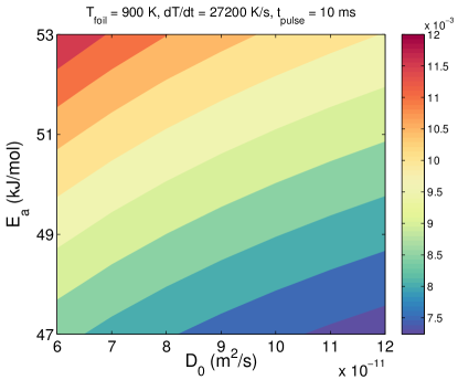
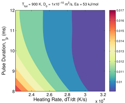
(a) Model	(b) PC Surrogate

Figure 1: Contours of reaction time as function of the physical parameters $D_{0}$ and $E_{a}$ (top) and of the design variables $t_{p}$ and $dT/dt$ (bottom). The contours are generated using (a) the reaction model, and (b) the PC surrogate.

To quantify the variability induced by the design and physical parameters, we exploit the PC surrogates to estimate the associated Sobol sensitivity indices. Results are reported in Figure 2, which depicts the first order and total sensitivity indices associated with $D_{0}$, $E_{a}$, $dT/dt$ and $t_{p}$, based on the PC expansion for the 900 K reaction time.

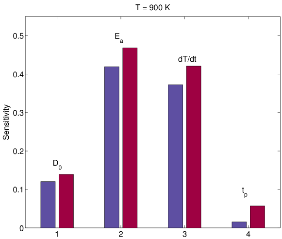
Figure 2: First order (blue) and total sensitivity (red) indices for the uncertain diffusivity parameters and design variables.

It is observed that the model predictions are predominantly sensitive to $E_{a}$ and $dT/dt$. This is consistent with the observations from Figure 1, as well as the analysis in [1] which considered the impact of $D_{0}$ and $E_{a}$ at fixed values of $t_{p}$ and $dT/dt$. In addition, we note that except for $t_{p}$, the first and total order sensitivity indices are close to each other indicating that the contributions due to mixed terms (joint effects) in the PC expansion are small. The observed trends underscore the importance of properly selecting the design conditions for the purpose of calibrating the model parameters, as discussed further below.

Additional insight into the variability induced by the parameters is gained by plotting PDFs of the reaction time. The PDFs are created by first generating a large number ($10^{5}$ – $10^{6}$) of MC samples of $\bm{\xi}$, evaluate the PC expansion at those points, and employ kernel density estimation on the outputs to create smooth density visualizations. Figure 3 depicts the PDFs for reaction time due to the uncertainty jointly over parameter and design spaces (4D case), and also for due to the uncertainty from only the parameter space and at a fixed setting of the heating rate and pulse duration (2D case). Plotted are curves generated based on PC representation of the 600K and 900K reaction times. As expected, the distributions corresponding to the 4D case (blue curves) exhibit a wider spread (variability) as compared to the 2D case (black curves). For both the 4D and 2D cases, the maximum likelihood estimate (MLE) of 900K reaction time is shifted to the right with respect to the MLE of the 600K reaction reaction time. Additionally, the standard deviation ($\sigma$) estimates indicate that the coefficients of variation associated with the distributions are large, corresponding to several fold variability in the reaction times.

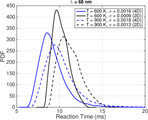
Figure 3: Probability density functions of the reaction time, generated using kernel density estimation. Plotted are curves generated for a multilayer with $\lambda=68$ nm using the 4D and 2D surrogates. The 2D surrogates are obtained from the 4D PC expansion by fixing the heating rate and pulse duration, respectively $t_{p}=10$ ms and $dT/dt=22200$ K/s. For each curve, the value of the standard deviation is indicated in the label.

We now explore the behavior of the expected utility function (7). In this work, we perform the optimization using a simple grid search; more sophisticated optimization algorithms may be employed, such as those described in [42], but we do not pursue them here. The 2D design space is discretized using a $20\times 20$ uniform grid, for a total of $N_{d}=400$ design points. At each design point, we compute a numerical approximation of $U(\bm{d})$ via (9) and (10), using $N_{out}=N_{in}=1000$ samples of the diffusion parameters. To generate the $\bm{y}$ samples, we first obtain our model evaluations $\bm{M}$ by evaluating the PC surrogate (note that the PC surrogate has replaced the expensive ODE models), and then substitute them into (11). The value of $\alpha$ was chosen to be 0.1 for the present exercise. Figure 4 illustrates contours of the expected utility generated using surrogates constructed at a reaction temperature of 900 K and a bilayer thickness of 72 nm. Results obtained using MC sampling and Latin Hypercube Sampling (LHS) agree well with each other. The design point, P, that maximizes the expected utility is located near the lower-left corner of the design space. In other words, experiments conducted at lower values of the heating rate and pulse duration are anticipated to be most informative. The expected utility function also drops rapidly as the pulse duration and heating rate increase, reaching a minimum near the top-right of the design space.

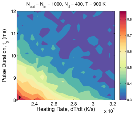
(a) Monte Carlo Sampling	(b) Latin Hypercube Sampling

Figure 4: Contours of the expected utility in the considered ranges of the design variables. Results are obtained using (a) Monte Carlo sampling and (b) Latin Hypercube sampling. In each case, the point P corresponds to the maximum utility value.

Figure 5 contrasts utility function contours for Zr-Al multilayers with bilayer thicknesses, $\lambda=68$ nm and 72 nm. Contours in both cases are qualitatively similar, and the more informative designs reside in regions of smaller values of heating rate and pulse duration. However, quantitative differences can be observed. These are indeed expected, as the reaction times are expected to depend significantly on the bilayer thickness [66, 36, 67, 68]. Highlighted in Figure 5(a) are two extreme scenarios corresponding to the maximum and minimum utility estimates. Design conditions at point P are regarded as optimal, whereas conditions at point R are expected to be least informative. The ratio of the expected utility estimated for the design P to that of design R is approximately 3.08 for the $\lambda$ = 72 nm case, and approximately 2 for the $\lambda$ = 68 nm case. Hence, the information gain from the posterior to the prior is expected to be much higher when data from optimally designed experiments is used for parameter inference.

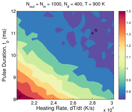
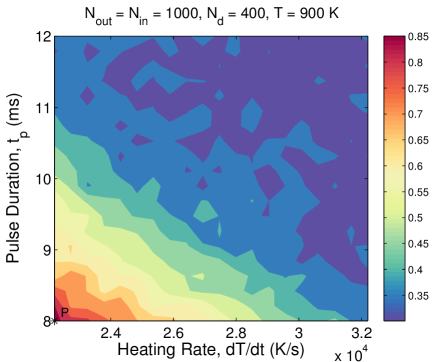
(a) $\lambda$ = 68 nm	(b) $\lambda$ = 72 nm

Figure 5: Contours of the expected utility for (a) $\lambda=68$ nm, and (b) $\lambda=72$ nm. In (a), the points P and R correspond to the maximum and minimum utility values, respectively.

To validate the predictions based on the utility function, a Bayesian inference exercise is conducted based on synthetic data, generated by taking $D_{0}=1\times 10^{-10}$ m²/s and $E_{a}=51$ kJ/mol as the “truth” parameter values. To generate the synthetic observations, we first evaluate the ODE model for the reaction time, $t_{r}$ at foil temperatures ranging from 700 K to 900 K, at increments of 5 K. The resulting reaction time estimates are then substituted into (11), and corrupted by a Gaussian noise ($\alpha$ = 0.01) to generate the set of experimental observations, $\bm{y}$. Joint posterior distributions of the diffusion parameters based on the synthetic observations are illustrated in Figure 6, for the two designs labeled in Figure 5(a). The inference results are consistent with the expected utility: the results in Figure 6 indicate a more concentrated (sharper) posterior distribution for design P than for R. However, in both cases, a small bias from the assumed truth is observed. This is expected since observations are noisy, and also because surrogates are used in lieu of full model computations in both the experimental design and inference phases.

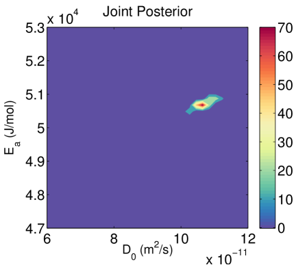
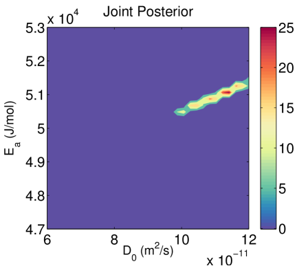
(a) P	(b) R

Figure 6: Joint posterior distribution of $D_{0}$ and $E_{a}$. Contours are generated for design conditions corresponding to (a) point P and (b) point R in Fig. 5(a).

To further investigate the inference results, we compare in Figure 7, the posterior marginals for $D_{0}$ and $E_{a}$ corresponding to the design conditions P and R. We observe that posterior marginals corresponding to design conditions P are much more concentrated than those corresponding to point R, again indicating that the former are indeed more informative. In addition, the maximum a posteriori (MAP) estimates in the case of the optimal design conditions are in better agreement with the assumed truth parameters.

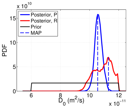
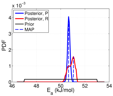
(a)	(b)

Figure 7: Marginal distribution of the posterior of (a) $D_{0}$ and (b) $E_{a}$. Curves are generated for design conditions corresponding to points P and R in Fig. 5(a). The uniform priors and the MAP estimates are also plotted.

4.2 Self-Propagating Reactions

For self-propagating front experiments, we again seek design conditions that maximize the expected information gain on $D_{0}$ and $E_{0}$. The design variables are now the initial foil temperature, $T_{0}$, and premix width, $w_{0}$. The parameters are assumed to have uniform priors in the following ranges: $D_{0}\in[1.5\times 10^{-9},4.5\times 10^{-9}]$ m²/s and $E_{a}\in[48,62]$ kJ/mol. The design variables are assigned uniform measures: $T_{0}\in[300,500]$ K and $w_{0}\in[0.5,1.5]$ nm. Our observable/QoI is the front velocity, $v$. Table 1 summarizes all the variables.

In this section, we apply a simplified approach to the design of self-propagating front experiments. The application of a simplified methodology is motivated by the fact that the front velocity is the main observable, and so a single experiment (performed using a nanolaminate foil of a specified bilayer thickness) yields a single data point only. One is thus faced with the challenge of dealing with a limited observation set, possibly involving noisy data. Several approaches have been applied to address this challenge, including performing repeated measurements at the same conditions, namely to quantify the impact of measurement uncertainty. Another avenue is based on the variation of foil properties. The most common approach falling within this framework concerns conducting experiments with different bilayer thicknesses. Whereas this approach has proven to be effective, it generally requires different deposition runs to synthesize samples with the desired properties, and to characterize the samples through imaging and calorimetry. These synthesis and analysis steps can be quite costly and time consuming, which leads to inherent constraints on the experimental sample size. An alternative approach is to conduct experiments with the same bilayer thickness but different premixed widths, which can be altered post fabrication through low-temperature annealing.

In light of the considerations above, we adopt a simplified approach that enables us to consider two different scenarios, and to draw inferences in an efficient manner. For each of these settings, we rely on a Bayesian inference methodology based on synthetic, noisy velocity data, and analyze the resulting information gain. In the first, we assume a design strategy in which experiments are conducted for multilayers with bilayer thicknesses falling at uniform intervals in a broad range. In the second scenario, a design methodology is assumed in which repeated measurements are conducted for samples having disparate values of the bilayer thickness. In addition, we assess the impact of sample size of the available measurements, and of measurement uncertainty on posterior marginals of the diffusion parameters. We then contrast posterior marginals pertaining to the two different strategies. As in the analysis above, we rely on PC surrogates of the observable in order to enable efficient sampling of posterior distributions.

We then construct PC surrogates for the self-propagating front velocity according to:

$$v(\lambda)=\sum_{\bm{k}=0}^{P}c_{\bm{k}}(\lambda)\Psi_{\bm{k}}(\bm{\xi})$$ (17)

where $\bm{\xi}$ is four-dimensional corresponding to the stochastic degrees of freedom in $D_{0}$, $E_{a}$, $T_{0}$, $w_{0}$. The coefficients $c_{k}$ are computed using the aPSP algorithm, requiring 36 iterations and a total of 2225 independent model simulations. The four-dimensional polynomial basis of the resulting surrogate in this case is observed to be of the order: 2, 2, 6 and 2 along $\xi_{1}$, $\xi_{2}$, $\xi_{3}$ and $\xi_{4}$ respectively. Relative error is computed for surrogates generated for different bilayer thicknesses falling in the range 40 nm – 90 nm, and the peak value of the relative error is found to be less than 0.45%. The aPSP construction thus provides excellent representations of the reaction velocity behavior in all cases considered in the present setup.

Figure 8 illustrates reaction velocity contours for a Zr-Al multilayer with bilayer thickness, $\lambda=67.38$ nm. Plotted are 2D contours for the considered range of diffusion parameters using fixed values of the design parameters, and for the considered range of design conditions with fixed values of the diffusion parameters. The contours are generated directly from the realizations, and by sampling the PC representation of the front velocity on uniform grids. Furthermore, Figure 8 indicates that, as expected, the reaction velocity increases as the diffusivity pre-exponent increases, and decreases as the activation energy increases. In addition, the reaction velocity increases with $T_{0}$, and decreases with $w_{0}$. The results also show that contours generated directly from the simulation data are in close agreement with those obtained by sampling the PC representation. This is consistent with the PC relative errors.

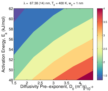
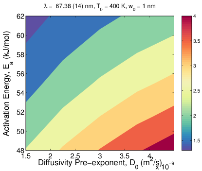
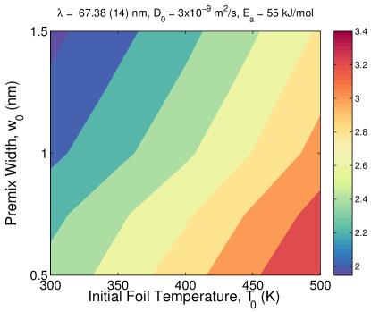
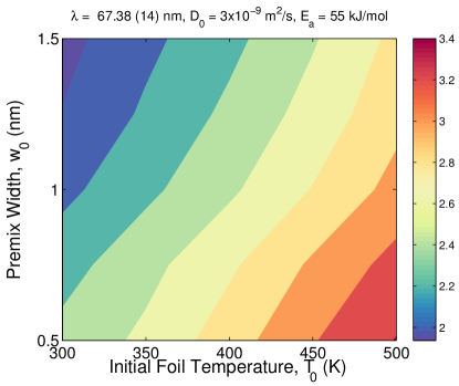
(a) Model	(b) PC Surrogate

Figure 8: Contours of reaction velocity as function of the physical parameters, $D_{0}$ and $E_{a}$ (top) and of the design variables, $t_{p}$ and $dT/dt$ (bottom). The contours are generated using (a) the reaction model, and (b) the PC surrogate.

Plotted in Figure 9 are PDFs of reaction velocity as a result of uncertainty in both the parameters and design variables, and generated using PC surrogates constructed for four different values of $\lambda$. The predictions reveal that the peak of the distribution shifts towards lower velocities as $\lambda$ increases. This is consistent with previous experimental, analytical and computational results [69, 29, 20, 1], which indicate that the front velocity decreases with bilayer thickness, as long as the latter is sufficiently larger than the thickness of the premixed layer. The spread in the distributions, as quantified by the standard deviation, $\sigma$, is also observed to decrease with $\lambda$. However, for the range of parameters and bilayers considered, the coefficient of variation, defined as the ratio of the standard deviation to the mean, is observed to be tightly bounded in the range $[0.2635,0.2714]$. Thus, the variability of the front velocity over the considered parameters domains has similar impact for the entire range of bilayers considered.

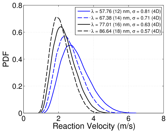
Figure 9: PDFs of reaction velocity for $\lambda=57.76$ nm, 67.38 nm, 77.01 nm and 86.64 nm. Reported in brackets is the corresponding thickness of the aluminum layer in each case.

To validate our approach involving parameter inference in a Bayesian setting, we perform a posterior predictive check using two different values of the premix width, $w_{0}=1.39$ nm, and $w_{0}=0.6$ nm. For each bilayer thickness considered, MCMC samples are used to determine the mean value and standard deviation of the reaction velocity. The posterior predictive results are contrasted with the original data used in the inference, as illustrated in Figure 10. It is seen that in all cases the posterior predictive captures the data within reasonable bounds. This provides confidence in the inferred diffusion parameters and corresponding velocity estimates.

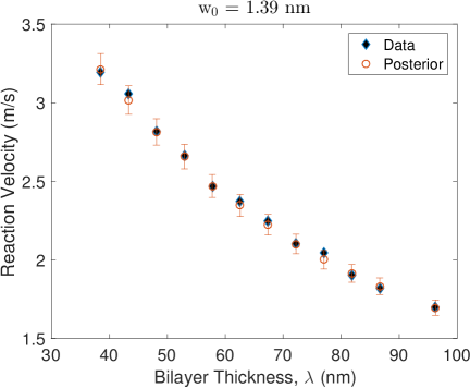
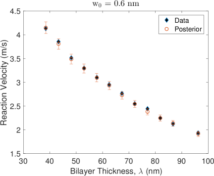
(a)	(b)

Figure 10: Reaction velocity versus bilayer thickness for (a) $w_{0}=1.39$ nm, and (b) $w=0.6$ nm. The synthetic data is depicted using symbols. The vertical bars correspond to $\pm 1$ standard deviation of the posterior predictive.

The first and total order Sobol sensitivity indices for the four uncertain parameters are shown using bar graphs in Figure 11. It is seen that the model predictions for reaction velocity are most sensitive to $E_{a}$, followed by $D_{0}$, $T_{0}$ and $w_{0}$. Specifically, the sensitivity indices of $E_{a}$ and $D_{0}$ are large, and so the impact of these parameters is clearly dominant. The sensitivity indices of $T_{0}$ and $w_{0}$ are relatively smaller, but their impact is still significant. The results in Figure 11 also show that first-order and total sensitivity indices of all four parameters are close to each other, which indicates a small contribution from mixed terms to the variance of the front velocity. Thus, in the parameter range considered, the contributions of individual parameters are in large part additive. This is not surprising because variations of the premixed width and initial temperature are naturally restricted to relatively small ranges.

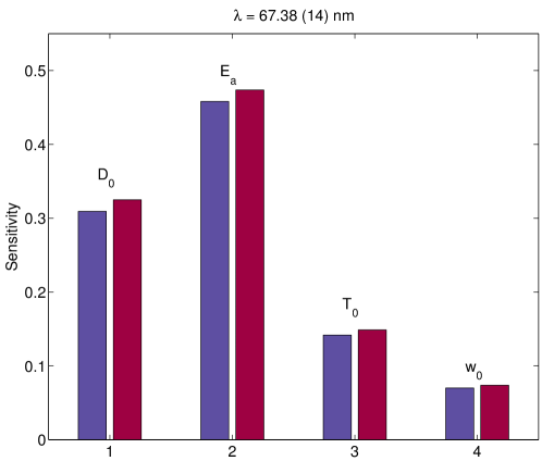
Figure 11: First order (blue) and total sensitivity (red) indices for the uncertain diffusivity parameters and design variables.

In order to assess the expected information gain associated with different design scenarios, we generate noisy synthetic data for the reaction velocity. The data are generated based on the PC representation of the model predictions, assuming “truth” diffusion parameter values of $D_{0}=3\times 10^{-9}$ m²/s and $E_{a}=55$ kJ/mol. The predictions are then perturbed with a Gaussian noise, using $\alpha=0.05$ in (11). The resulting synthetic velocity observations, plotted in Figure 12 for a range of bilayers, are then used as data for the Bayesian calibration step. As further discussed below, we contrast this $v$-$\lambda$ experimental design with alternatives based on similarly observing the reaction velocity for a range of initial foil temperatures ($v$-$T_{0}$ design), and a range of premix widths ($v$-$w_{0}$ design).

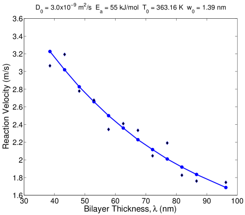
Figure 12: Reaction velocity versus bilayer thickness. The solid curve and circular dots corresponds to model results generated in the range, 40 nm $\leq\lambda\leq 100$ nm. The diamond symbols are perturbed values corresponding to a multiplicative Gaussian noise with a standard deviation of 5% of the unperturbed model estimate.

Figure 13 shows posterior marginal distributions of the activation energy for $v$-$\lambda$ and $v$-$w_{0}$ designs. Plotted are curves generated for different samples sizes, namely 4 and 12 for the $v$-$\lambda$ design, and 5 and 20 for the $v$-$w_{0}$ design. The results indicate that for both designs, under the present noise conditions, the larger sample size leads to a significantly sharper posterior than when the smaller sample size is used. In addition, the MAP estimate is closer to the assumed truth value, though evidently a discrepancy is still observed. The discrepancy arises due to measurement noise and PC approximation error, and generally would only vanish in the limit of infinite data and infinite polynomial order in PC surrogates.

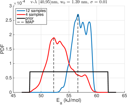
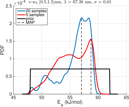
(a)	(b)

Figure 13: Marginal distributions of the posterior of the activation energy. Results are generated based on (a) $v$-$\lambda$ data pairs, and (b) $v$-$w_{0}$ data pairs. Curves are generated for different size data, as indicated. The uniform priors and MAP estimates are also plotted.

To assess the impact of observation noise, we generate posterior marginals of $E_{a}$ for the $v$-$\lambda$ design and different values of $\sigma$. Figure 14 contrasts posterior marginals obtained with $\alpha=0.05$ and 0.01. The distribution corresponding to a lower noise is observed to be much sharper. In other words, we obtain much tighter bounds on the estimates of $E_{a}$ when measurement uncertainty is reduced. Moreover, it is found that MAP estimates are closer to the truth value of 55 kJ/mol when sample size is increased and observation noise is reduced. Note that in the results presented above and later in this section, we show posterior marginals of $E_{a}$ only, as similar trends exist for $D_{0}$ and so we omit them for brevity.

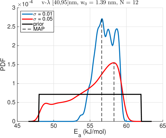
Figure 14: Marginal distributions of the posterior of $E_{a}$ for different values of the noise level.

We now contrast posterior marginals for three different scenarios, namely based on $v$-$\lambda$, $v$-$w_{0}$ and $v$-$T_{0}$ designs. In all cases, the sample size ($N$ = 5) and observation noise ($\alpha=0.01$) are held fixed. Moreover, the range of values for $\lambda$, $T_{0}$ and $w_{0}$ are selected such that the reaction velocity varies in the approximate range 2.2–2.7 m/s. Figure 15 depicts the marginal posterior distributions of $E_{a}$ for all three designs. The results show that for the case of $v$-$\lambda$ distribution, the information gain is highest followed by $v$-$T_{0}$ and $v$-$w_{0}$. Moreover, the MAP estimate for the $v$-$\lambda$ case is found to be closest to the assumed truth value, 55 kJ/mol. Thus, it is seen that under the present constraints, performing reaction velocity measurements by varying the bilayer would be more informative than experimental designs based on varying the initial temperature or premix width. As noted earlier, however, varying the bilayer would generally require a higher effort in synthesizing and characterizing the requisite number of samples.

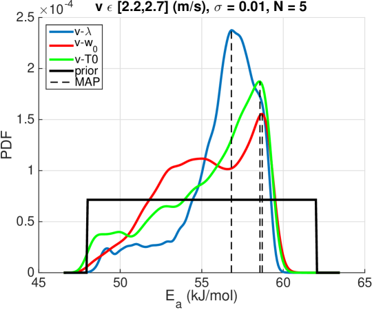
Figure 15: Marginal distributions of the posterior of $E_{a}$ based on $v$-$\lambda$, $v$-$w_{0}$ and $v$-$T_{0}$ data pairs. The uniform prior and MAP values are also plotted.

As a possible cost-effective alternative to performing experiments at different bilayer thicknesses, we consider the possibility of performing repeated experiments at two disparate values of the bilayer thickness. This is motivated by recent experiences of optimal experimental design of shock tube experiments [70], which aimed at maximizing the information gain resulting from a fixed number of experiments. The results in [70] showed that an attractive strategy is based on repeated experiments at high and low values of temperature, namely because these designs are effective in isolating the impact of observation noise and consequently in estimating the rate parameters. In the context of reactive multilayers, such a strategy would offer the advantage of minimizing the number of fabrication runs.

We explore the suitability of this approach by generating multiple realizations of the synthetic velocity data at low and high values of the bilayer, and contrast this design to one in which single observations are made at distinct values of the bilayer that are uniformly distributed in the range bounded by the low and high bilayer values. The synthetic velocity data thus generated are illustrated in Figures 16(a) and (b) respectively. Note that in both cases the sample size (= 10) is held fixed. Specifically, in the repeated experiment design, 5 observations are collected at each of the high and low values of $\lambda$. Shown in Figure 16(c) are the posterior marginal distributions of the activation energy for the two designs shown in Figures 16(a) and (b). The results indicate that posterior distributions for both cases are very close. The corresponding MAP estimates are also in agreement. This indicates that both strategies provide effective means of calibrating the diffusion parameters, with close estimates of the information gain. However, as noted above, in the present exercise the repeated observation design would be more cost effective than the uniformly distributed bilayer design, because two distinct fabrication runs would be required in the former whereas ten would be needed in the latter.

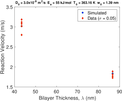
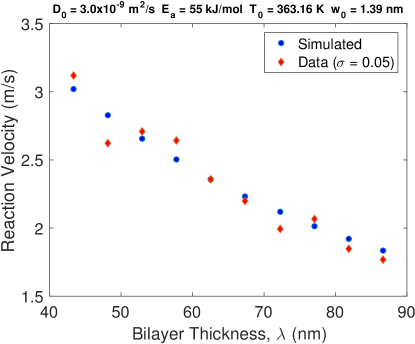
(a)	(b)

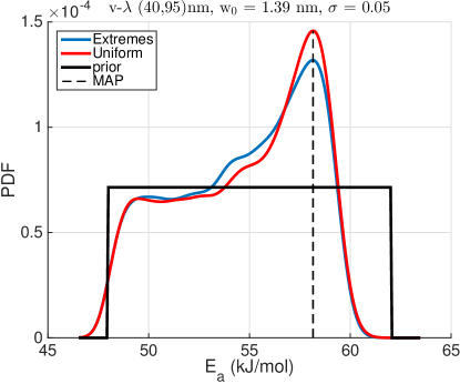
(c)

Figure 16: (a) Simulated and perturbed reaction velocities for $\lambda=43.32$ nm and $\lambda=86.64$ nm. (b) Simulated and perturbed reaction velocities for a range of bilayers uniformly distributed in the range, 43.32 nm $\leq\lambda\leq 86.64$ nm. (c) Marginal distributions of the posterior for $E_{a}$ based on the synthetic perturbed data pairs shown in (a) and (b).

5 Conclusions

We presented a Bayesian approach for systematically designing optimal reactive multilayer experiments. We focused on Zr-Al multilayers with a 1:1 molar ratio, and considered both homogeneous ignition and self-propagation experiments for the goal of learning about the uncertain Arrhenius parameters that describe the behavior of the atomic intermixing rates. For the homogeneous ignition experiment, the design variables are heating rate and pulse duration, and the observable is the characteristic time of the transient temperature profile during the ignition. For the self-propagation experiment, the design variables are initial foil temperature and premix width, and the observable is the front velocity. We also explore the design effects of bilayer thickness.

The optimal experimental design methodology employs an objective function (expected utility function) based on the Kullback-Leibler divergence between posterior and priors, reflecting the expected information gain on the uncertain parameters from the noisy measurements at a given design condition; the goal is then to find the design that maximizes this quantity. The expected utility is estimated numerically using a doubly-nested Monte Carlo formula. Its evaluation involves potentially thousands, millions, or even more solves of the physical model (ODE system), rendering it impractical. We thus construct a computationally-cheaper surrogate model based on polynomial chaos (PC) expansions, that capture the dependence of observables on both design and uncertain parameters. An adaptive pseudo-spectral projection technique is used to efficiently build accurate PC surrogates. The PC surrogates not only enable tractable optimal experimental design procedure, but also provide global sensitivity information and accelerate post-experiment Bayesian inference/calibration.

For the homogeneous ignition experiment, the design procedure reveals that the expected utility peaks as the heating rate and pulse duration decrease. These predictions are then verified using a Bayesian calibration exercise, based on synthetic noisy data generated from the PC surrogate assuming truth values of the activation energy and the pre-exponent. The inference is performed at optimal and non-optimal designs, and sharper posterior distributions are indeed obtained at the optimal design conditions.

For the self-propagation experiment, computations indicate that the expected information gain from experimental reaction velocity measurements increases as the sample size of the data increases and the measurement uncertainty decreases. The analysis also shows that reaction velocity measurements are more informative when conducted by varying the bilayer thicknesses as opposed to varying the initial foil temperature or the initial premix width. Additionally, the two design scenarios for $\lambda$ (uniformly discretized across a region versus repeated at two thicknesses) under fixed values of the data size and measurement uncertainty level and for the same assumed truth parameters, led to posterior distributions that are in close agreement. These results suggest that the repeated measurement approach can provide a cost-effective alternative to consideration of a large number of bilayers, as this generally entails a substantial synthesis cost.

In closing, we note that this study involves a number of assumptions, such as the lack of model error quantification and the use of an additive Gaussian noise structure. While these assumptions are reasonable for our present purpose, more advanced techniques on these fronts are certainly of great interest and value, and would be natural additions to the current framework. Finally, development of the optimal experimental design formulation and algorithms for multiple experiments, especially in a sequential manner that makes use of information feedback, can lead to even greater gains [71].

References

- [1] M. Vohra, J. Winokur, K.R. Overdeep, P. Marcello, T.P. Weihs, and O.M. Knio. Development of a reduced model of formation reactions in Zr-Al nanolaminates. Journal of Applied Physics, 116(23):233501, 2014.
- [2] K.J. Blobaum, D. Van Heerden, A.J. Gavens, and T.P. Weihs. Al/Ni formation reactions: characterization of the metastable Al9Ni2 phase and analysis of its formation. Acta Materialia, 51(13):3871 – 3884, 2003.
- [3] J.S. Kim, T. LaGrange, B.W. Reed, R. Knepper, T.P. Weihs, N.D. Browning, and G.H. Campbell. Direct characterization of phase transformations and morphologies in moving reaction zones in Al/Ni nanolaminates using dynamic transmission electron microscopy. Acta Materialia, 59(9):3571 – 3580, 2011.
- [4] J.C. Trenkle, J. Wang, T.P. Weihs, and T.C. Hufnagel. Microstructural study of an oscillatory formation reaction in nanostructured reactive multilayer foils. Applied Physics Letters, 87(15):153108–153108, 2005.
- [5] J.C. Trenkle, L.J. Koerner, M.W. Tate, S.M. Gruner, T.P. Weihs, and T.C. Hufnagel. Phase transformations during rapid heating of Al/Ni multilayer foils. Applied Physics Letters, 93(8):081903–081903, 2008.
- [6] A.J. Swiston, E. Besnoin, A. Duckham, O.M. Knio, T.P. Weihs, and T.C. Hufnagel. Thermal and microstructural effects of welding metallic glasses by self-propagating reactions in multilayer foils. Acta Materialia, 53:3713–3719, 2005.
- [7] A. Duckham, J. Newson, M.V. Brown, T.R. Rude, O.M. Knio, E.M. Heian, and J.S. Subramanian. Method for fabricating large dimension bonds using reactive multilayer joining. U.S. Patent 7,354,659, 2008.
- [8] G. Van Heerden, J. Newson, T. Rude, O.M. Knio, and T.P. Weihs. Methods and device for controlling pressure in reactive multilayer joining and resulting product. U.S. Patent 7,441,688, 2008.
- [9] J. Wang, E. Besnoin, O.M. Knio, and T.P. Weihs. Nanostructured soldered or brazed joints made with reactive multilayer foils. U.S. Patent 7,361,412, 2008.
- [10] G. Van Heerden, D. Deger, T.P. Weihs, and O.M. Knio. Hermetically sealing a container with crushable material and reactive multilayer material. U.S. Patent 7,143,568, 2006.
- [11] G. Van Heerden, D. Deger, T.P. Weihs, and O.M. Knio. Container hermetically sealed with crushable material and reactive multilayer material. U.S. Patent 7,121,402, 2006.
- [12] A.G. Merzhanov. Self-propagating high-temperature synthesis: Twenty years of search and findings. In Z.A. Munir and J.B. Holt, editors, Combustion and Plasma Synthesis of High-Temperature Materials. VCH Publishers, NY, 1990.
- [13] M. Koizumi and Y. Miyamoto. Recent progress in combustion synthesis of high-performance materials in Japan. In Z.A. Munir and J.B. Holt, editors, Combustion and Plasma Synthesis of High-Temperature Materials. VCH Publishers, NY, 1990.
- [14] H. Joress, S.C. Barron, K.J.T. Livi, N. Aronhime, and T.P. Weihs. Self-sustaining oxidation initiated by rapid formation reactions in multilayer foils. Applied Physics Letters, 101(11):111908–111908, 2012.
- [15] M. Vohra, T.P. Weihs, and O.M. Knio. A simplified computational model of the oxidation of Zr/Al multilayers. Combustion and Flame, 162(1):249–257, 2014.
- [16] K.R. Overdeep, K.J.T. Livi, D.J. Allen, N.G. Glumac, and T.P. Weihs. Using magnesium to maximize heat generated by reactive Al/Zr nanolaminates. Combustion and Flame, 162(7):2855–2864, 2015.
- [17] J. Feng, G. Jian, Q. Liu, and M.R. Zachariah. Passivated iodine pentoxide oxidizer for potential biocidal nanoenergetic applications. ACS applied materials & interfaces, 5(18):8875–8880, 2013.
- [18] K.T. Sullivan, N.W. Piekiel, S. Chowdhury, C. Wu, M.R. Zachariah, and C.E. Johnson. Ignition and combustion characteristics of nanoscale Al/AgIO3: A potential energetic biocidal system. Combustion Science and Technology, 183(3):285–302, 2010.
- [19] A.J. Gavens, D. Van Heerden, A.B. Mann, M.E. Reiss, and T.P. Weihs. Effect of intermixing on self-propagating exothermic reactions in Al/Ni nanolaminate foils. Journal of Applied Physics, 87(3):1255–1263, 2000.
- [20] E. Besnoin, S. Cerutti, O.M. Knio, and T.P. Weihs. Effect of reactant and product melting on self-propagating reactions in multilayer foils. J. Appl. Phys., 92:5474–5481, 2002.
- [21] E. Ma, C.V. Thompson, L.A. Clevenger, and K.N. Tu. Self-propagating explosive reactions in Al/Ni multilayer thin films. Applied physics letters, 57(12):1262–1264, 1990.
- [22] M.E. Reiss, C.M. Esber, D. Van Heerden, A.J. Gavens, M.E. Williams, and T.P. Weihs. Self-propagating formation reactions in Nb/Si multilayers. Mat. Sci. Eng., A261:217–222, 1999.
- [23] J. Wang, E. Besnoin, O.M. Knio, and T.P. Weihs. Investigating the effect of applied pressure on reactive multilayer foil joining. Acta Materialia, 52(18):5265 – 5274, 2004.
- [24] A.S. Rogachev, A.É. Grigoryan, E.V. Illarionova, I.G. Kanel, A.G. Merzhanov, A.N. Nosyrev, N.V. Sachkova, V.I. Khvesyuk, and P.A. Tsygankov. Gasless combustion of Ti-Al bimetallic multilayer nanofoils. Combustion, Explosion, and Shock Waves, 40:166–171, 2004.
- [25] J. Gachon, A. Rogachev, H. Grigoryan, E. Illarionova, J. Kuntz, D. Kovalev, A. Nosyrev, N. Sachkova, and P. Tsygankov. On the mechanism of heterogeneous reaction and phase formation in Ti/Al multilayer nanofilms. Acta. Mater, 53:1225–1231, 2005.
- [26] D.P. Adams, M.M. Bai, M.A. Rodriguez, J.J. Moore, L.N. Brewer, and J.B. Kelley. Structure and properties of Ni-Ti thin films used for brazing. In J.J. Stephens and K.S. Weil, editors, Proceedings of the 3rd International Brazing and Soldering Conference, 2006.
- [27] D.P. Adams, M.A. Rodriguez, C.P. Tigges, and P.G. Kotula. Self-propagating, high-temperature combustion synthesis of rhombohedral Al-Pt thin films. J. Mater. Res., 21:3168–3179, 2006.
- [28] S. Jayaraman, A.B. Mann, O.M. Knio, G. Bao, and T.P. Weihs. Numerical modeling of self-propagating exothermic reactions in multilayer systems. In E. Ma, M. Atzmon, P. Bellon, and R. Trivedi, editors, MRS Symp. Proc. Vol. 481, page 563, 1998.
- [29] A.B. Mann, A.J. Gavens, M.E. Reiss, D. Van Heerden, G. Bao, and T.P. Weihs. Modeling and characterizing the propagation velocity of exothermic reactions in multilayer foils. Journal of Applied Physics, 82(3):1178–1188, 1997.
- [30] Z.A. Munir and J.B. Holt. Combustion and plasma synthesis of high-temperature materials. VCH New York etc., 1990.
- [31] M. Salloum and O.M. Knio. Simulation of reactive nanolaminates using reduced models: I. Basic formulation. Combustion and Flame, 157(2):288–295, 2010.
- [32] M. Salloum and O.M. Knio. Simulation of reactive nanolaminates using reduced models: II. Normal propagation. Combustion and Flame, 157(3):436–445, 2010.
- [33] M. Salloum and O.M. Knio. Simulation of reactive nanolaminates using reduced models: III. Ingredients for a general multidimensional formulation. Combustion and Flame, 157(6):1154–1166, 2010.
- [34] L. Alawieh, O.M. Knio, and T.P. Weihs. Effect of thermal properties on self-propagating fronts in reactive nanolaminates. Journal of Applied Physics, 110(1):013509, 2011.
- [35] I. Sraj, M. Vohra, L. Alawieh, T.P. Weihs, and O.M. Knio. Self-propagating reactive fronts in compacts of multilayered particles. Journal of Nanomaterials, 2013:13, 2013.
- [36] G.M. Fritz. Characterizing the ignition threshold of multilayer reactive materials and controlling reaction velocities in compacts of reactive laminate particles. Ph.D. thesis, The Johns Hopkins University, 2011.
- [37] L. Alawieh, T.P. Weihs, and O.M. Knio. A generalized reduced model of uniform and self-propagating reactions in reactive nanolaminates. Combustion and Flame, 160(9):1857–1869, 2013.
- [38] X. Huan and Y.M. Marzouk. Simulation-based optimal bayesian experimental design for nonlinear systems. Journal of Computational Physics, 232(1):288–317, 2013.
- [39] S. Jayaraman, A.B. Mann, M. Reiss, T.P. Weihs, and O.M. Knio. Numerical study of the effect of heat losses on self-propagating reactions in multilayer foils. Combust. Flame, 124:178–194, 2001.
- [40] K. Chaloner and I. Verdinelli. Bayesian Experimental Design: A Review. Statistical Science, 10(3):273–304, 1995.
- [41] P. Müller. Simulation Based Optimal Design. Handbook of Statistics, 25:509–518, 2005.
- [42] X. Huan and Y.M. Marzouk. Gradient-Based Stochastic Optimization Methods in Bayesian Experimental Design. International Journal for Uncertainty Quantification, 4(6):479–510, 2014.
- [43] J.O. Berger. Statistical decision theory and Bayesian analysis. Springer, 1985.
- [44] E.S. Epstein. Statistical inference and prediction in climatology: a Bayesian approach. Meteorological monographs (USA), 1985.
- [45] D.S. Sivia. Data analysis: a Bayesian tutorial. Oxford university press, 1996.
- [46] D.V. Lindley. On a Measure of the Information Provided by an Experiment. The Annals of Mathematical Statistics, 27(4):986–1005, 1956.
- [47] D.V. Lindley. Bayesian Statistics: A Review. SIAM (Society for Industrial and Applied Mathematics), Philadelphia, PA, 1972.
- [48] K.J. Ryan. Estimating Expected Information Gains for Experimental Designs With Application to the Random Fatigue-Limit Model. Journal of Computational and Graphical Statistics, 12(3):585–603, 2003.
- [49] N. Wiener. The homogeneous chaos. American Journal of Mathematics, pages 897–936, 1938.
- [50] R.G. Ghanem and P.D. Spanos. Stochastic finite elements: a spectral approach, volume 387974563. Springer, 1991.
- [51] O.P. Le Maître and O.M. Knio. Spectral methods for uncertainty quantification: with applications to computational fluid dynamics. Springer, 2010.
- [52] D. Xiu and G.E. Karniadakis. The wiener–askey polynomial chaos for stochastic differential equations. SIAM Journal on Scientific Computing, 24(2):619–644, 2002.
- [53] P.G. Constantine, M.S. Eldred, and E.T. Phipps. Sparse pseudospectral approximation method. Computer Methods in Applied Mechanics and Engineering, 229-232:1–12, 2012.
- [54] P.R. Conrad and Y.M. Marzouk. Adaptive smolyak pseudospectral approximations. SIAM Journal on Scientific Computing, 35(6):A2643–A2670, 2013.
- [55] J. Winokur, P. Conrad, I. Sraj, O. Knio, A. Srinivasan, W.C. Thacker, Y. Marzouk, and M. Iskandarani. A priori testing of sparse adaptive polynomial chaos expansions using an ocean general circulation model database. Computational Geosciences, 17(6):899–911, 2013.
- [56] S.A. Smolyak. Quadrature and interpolation formulas for tensor products of certain classes of functions. In Dokl. Akad. Nauk SSSR, volume 4, page 123, 1963.
- [57] T. Crestaux, O. Le Maître, and J.M. Martinez. Polynomial chaos expansion for sensitivity analysis. Reliability Engineering & System Safety, 94(7):1161–1172, 2009.
- [58] T. Homma and A. Saltelli. Importance measures in global sensitivity analysis of nonlinear models. Reliability Engineering & System Safety, 52(1):1–17, 1996.
- [59] I.M. Sobol′. Global sensitivity indices for nonlinear mathematical models and their monte carlo estimates. Mathematics and Computers in Simulation, 55(1-3):271–280, 2001.
- [60] B. Sudret. Global sensitivity analysis using polynomial chaos expansions. Reliability Engineering & System Safety, 93(7):964–979, 2008.
- [61] A. Alexanderian, J. Winokur, I. Sraj, A. Srinivasan, M. Iskandarani, W.C. Thacker, and O.M. Knio. Global sensitivity analysis in an ocean general circulation model: a sparse spectral projection approach. Computational Geosciences, 16:757–778, 2012.
- [62] H. Haario, E. Saksman, J. Tamminen, et al. An adaptive metropolis algorithm. Bernoulli, 7(2):223–242, 2001.
- [63] Y.M. Marzouk, H.N. Najm, and L.A. Rahn. Stochastic spectral methods for efficient bayesian solution of inverse problems. Journal of Computational Physics, 224(2):560–586, 2007.
- [64] Y.M. Marzouk and H.N. Najm. Dimensionality reduction and polynomial chaos acceleration of bayesian inference in inverse problems. Journal of Computational Physics, 228(6):1862–1902, 2009.
- [65] T.N.L Patterson. The optimum addition of points to quadrature formulae. Mathematics of Computation, 22(104):847–856, 1968.
- [66] G.M. Fritz, S.J. Spey, M.D. Grapes, and T.P. Weihs. Thresholds for igniting exothermic reactions in Al/Ni multilayers using pulses of electrical, mechanical, and thermal energy. Journal of Applied Physics, 113(1):014901, 2013.
- [67] C.J. Morris, B. Mary, E. Zakar, S. Barron, G. Fritz, O. Knio, T.P. Weihs, R. Hodgin, P. Wilkins, and C. May. Rapid initiation of reactions in al/ni multilayers with nanoscale layering. Journal of Physics and Chemistry of Solids, 71:84–89, 2010.
- [68] S.J. Spey. Ignition properties of multilayer nanoscale reactive foils and the properties of metal-ceramic joints made with the same. Ph.D. thesis, The Johns Hopkins University, 2006.
- [69] R. Knepper, M.R. Snyder, G.M. Fritz, K. Fisher, O.M. Knio, and T.P. Weihs. Effect of varying bilayer spacing distribution on reaction heat and velocity in reactive Al/Ni multilayers. Journal of Applied Physics, 105(8):083504, 2009.
- [70] F. Bisetti, D. Kim, O. Knio, Q. Long, and R. Tempone. Optimal bayesian experimental design for priors of compact support with application to shock-tube experiments for combustion kinetics. International Journal for Numerical Methods in Engineering, page in press, 2016.
- [71] X. Huan and Y.M. Marzouk. Sequential Bayesian optimal experimental design via approximate dynamic programming. arXiv preprint arXiv:1604.08320, 2016.