Best Subset Binary Prediction

Abstract

We consider a variable selection problem for the prediction of binary outcomes. We study the best subset selection procedure by which the covariates are chosen by maximizing Manski (1975, 1985)’s maximum score objective function subject to a constraint on the maximal number of selected variables. We show that this procedure can be equivalently reformulated as solving a mixed integer optimization problem, which enables computation of the exact or an approximate solution with a definite approximation error bound. In terms of theoretical results, we obtain non-asymptotic upper and lower risk bounds when the dimension of potential covariates is possibly much larger than the sample size. Our upper and lower risk bounds are minimax rate-optimal when the maximal number of selected variables is fixed and does not increase with the sample size. We illustrate usefulness of the best subset binary prediction approach via Monte Carlo simulations and an empirical application of the work-trip transportation mode choice.

Keywords: binary choice, maximum score estimation, best subset selection, $\ell_{0}$-constrained maximization, mixed integer optimization, minimax optimality, finite sample property

JEL codes: C52, C53, C55

1 Introduction

Prediction of binary outcomes is an important topic in economics and various scientific fields. Let $Y\in\{0,1\}$ be the binary outcome of interest and $W$ a vector of covariates for predicting $Y$. Assume that the researcher has a training sample of $n$ independent identically distributed (i.i.d.) observations $\left(Y_{i},W_{i}\right)_{i=1}^{n}$ of $(Y,W)$. For $w\in\mathcal{W}$, let

$$b_{\theta}(w)\equiv 1\left\{w^{\prime}\theta\geq 0\right\},$$ (1.1)

where $\mathcal{W}$ is the support of $W$, $\theta$ is a vector of parameters, and $1\left\{\cdot\right\}$ is an indicator function that takes value 1 if its argument is true and 0 otherwise.

One reasonable prediction rule is to choose $\theta$ such that it maximizes the probability of making the correct prediction $P\left[Y=b_{\theta}(W)\right]$. However, this is infeasible in practice since the joint distribution of $(Y,W)$ is unknown. A natural sample analog is to maximize the sample average score which equals the proportion of correct predictions under the prediction rule (1.1) in the training sample. This maximization problem is equivalent to the maximum score estimation in binary response models and is pioneered by Manski (1975, 1985). Thus, we call the corresponding prediction rule the maximum score prediction rule. See Manski and Thompson (1989), Jiang and Tanner (2010), and Elliott and Lieli (2013) for prediction in the maximum score approach.

This prediction problem has the same structure as the binary classification problem, which is extensively studied in the statistics and machine learning literature. For example, see the classic work of Devroye, Györfi, and Lugosi (1996) among many others. In this literature, the empirical risk minimization (ERM) classifier over the class of binary classifiers specified by (1.1) is defined as a minimizer of the empirical predictive risk, which is taken to be one minus the objective function of the maximum score prediction problem. In other words, the ERM classification rule is identical to the maximum score prediction rule.

In this paper, we address the covariate selection issue in the framework of predicting the binary outcome $Y_{i}$ using the class of linear threshold-crossing prediction rules $b_{\theta}(W_{i})$ defined by (1.1). We study the best subset selection procedure by which the covariates are chosen among a collection of candidate explanatory variables by maximizing the empirical score subject to a constraint on the maximal number of selected variables. In other words, we investigate theoretical and numerical properties of the $\ell_{0}$-norm constrained maximum score prediction rules.

To the best of our knowledge, Greenshtein (2006) and Jiang and Tanner (2010) are the only existing papers in the literature that explicitly considered the same prediction problem as ours. Greenshtein (2006) considered a general loss function that includes maximum score prediction as a special case in the i.i.d. setup. Greenshtein (2006) focused on a high dimensional case and established conditions under which the excess risk converges to zero as $n\rightarrow\infty$. Jiang and Tanner (2010) focused on the prediction of time series data and obtained an upper bound for the excess risk. Neither Greenshtein (2006) nor Jiang and Tanner (2010) provided any numerical results for the best subset maximum score prediction rule. In contrast, we focus on cross-sectional applications and emphasize computational aspects.

The main contributions of this paper are twofold: first, we show that the best subset maximum score prediction rule is minimax rate-optimal and second, we demonstrate that it can be implemented via mixed integer optimization. The first contribution is theoretical and builds on the literature of empirical risk minimization (Tsybakov, 2004; Massart and Nédélec, 2006, in particular). Specifically, we obtain non-asymptotic upper and lower risk bounds when the dimension of potential covariates is possibly much larger than the sample size $n$. Our upper and lower risk bounds are minimax rate-optimal when the maximal number of selected variables is fixed and does not increase with $n$. The existing results of finite-sample upper and lower risk bounds for the binary prediction problem focus on the case where there is no variable selection and the set of covariates is fixed and low-dimensional. Our risk bound results extend to the setup under the $\ell_{0}$-norm constraint when the set of potential covariates is high-dimensional.

The second contribution is computational. We face two kinds of computational challenges. One challenge comes from the nature of the objective function and the other is from the best subset selection. The maximum score objective function is a piecewise constant function whose range set contains only finitely many points. Hence the maximum of the score maximization problem is always attained yet the maximizer is generally not unique. It is known that computing the maximum score estimates regardless of the presence of the $\ell_{0}$ constraint is NP (non-deterministic polynomial-time)-hard (see, e.g., Johnson and Preparata, 1978). See Manski and Thompson (1986) and Pinkse (1993) for first generation algorithms for maximum score estimation.

Our computation algorithm is based on the method of mixed integer optimization (MIO). Florios and Skouras (2008) provided compelling numerical evidence that the MIO approach is superior to the first-generation approaches. Kitagawa and Tetenov (2018) used an MIO formulation that is different from Florios and Skouras (2008) to solve maximum score type problems. The objective of interest in Kitagawa and Tetenov (2018) is to develop treatment choice rules by maximizing an empirical welfare criterion, which resembles the maximum score objective function. They derived minimax optimality and used the MIO formulation to implement their algorithm. Neither Florios and Skouras (2008) nor Kitagawa and Tetenov (2018) were concerned with the variable selection problem.

These second generation approaches are driven by developments in MIO solvers and also by availability of a much faster computer compared to the period when the first generation algorithms were proposed. Florios and Skouras (2008) reported that they obtained the exact maximum score estimates using Horowitz (1993)’s data in 10.5 hours. In this application, the sample size was $n=842$ and there were 4 parameters to estimate.

It is well known that use of a good and tighter parameter space can strengthen the performance of a global optimization procedure including the MIO approach. In this paper, we propose a data driven approach to refine the parameter space. Using a state-of-the-art MIO solver as well as a tailor-made heuristic to choose the parameter space, it took us less than 5 minutes to obtain the exact maximum score estimates using the same dataset with the same number of parameters to estimate. This is a dramatic improvement at the factor of more than 100 relative to the numerical performance reported in Florios and Skouras (2008). In other words, we demonstrate that hardware improvements combined with the advances in MIO solvers and also with a carefully chosen parameter space have made the maximum score approach empirically much more relevant now than ten years ago.

The second numerical challenge is concerned with constrained optimization with the $\ell_{0}$-norm constraint. It is well known that the $\ell_{0}$-norm constraint renders the variable selection problem NP-hard even in the regression setup where the objective function is convex and smooth (see, e.g., Natarajan, 1995; Bertsimas, King, and Mazumder, 2016). Recently Bertsimas, King, and Mazumder (2016) proposed a novel MIO approach to the best subset variable selection problem when least squares and least absolute deviation risks are concerned. They demonstrated that the MIO approach can efficiently deliver a provably optimal solution to the resulting $\ell_{0}$-norm constrained risk minimization problem for a variety of datasets with practical problem size. Our implementation of the best subset maximum score prediction rules combines insights from Bertsimas, King, and Mazumder (2016), Florios and Skouras (2008), and Kitagawa and Tetenov (2018). We present two alternative MIO solution methods that complement each other.

In practical applications, it is useful to consider an approximate solution by adopting an early termination rule. In our empirical application, by setting an explicitly pre-specified optimization error, we were able to obtain approximate maximum score estimates with Horowitz (1993)’s data in around 10 minutes when both an intercept term and one specific random covariate were always selected, and there were 9 additional auxiliary covariates that were subject to the constraint where at most 5 of them could be selected. This suggests that fast developments in computing environments will enable us to solve an empirical problem at a practically relevant scale in very near future. We provide additional numerical evidence in Monte Carlo experiments in a high-dimensional setup when the number of potential covariates is larger than the sample size.

The remainder of this paper is organized as follows. In Section 2, we describe our prediction rule. Section 3 establishes theoretical properties of the proposed prediction rule. In Section 4, we present computation algorithms using the MIO approach, and in Section 5, we conduct a simulation study on the performance of our prediction rule in both low and high dimensional variable selection problems. In Section 6, we illustrate usefulness of our prediction rule in the empirical application of work-trip mode choice using Horowitz (1993)’s data. We then conclude the paper in Section 7. Proofs of all theoretical results and supplementary material of this paper are collated in online appendices.

2 A Best Subset Approach to Maximum Score Prediction of Binary Outcomes

In this section, we describe our proposal of the best subset maximum score prediction rule. Following Magnus and Durbin (1999) and Danilov and Magnus (2004), we distinguish between focus covariates that are always included in the prediction rule and auxiliary covariates of which we are less certain. We thus decompose the covariate vector $W$ as $W=(X,Z)$, where $X$ is a $\left(k+1\right)$-dimensional vector of focus covariates and $Z$ is a $p$-dimensional vector of auxiliary covariates.

Noting that $b_{a\theta}(w)=$ $b_{\theta}(w)$ for any positive real scalar $a$, we adopt the same scale normalization method as in Horowitz (1992) and Jiang and Tanner (2010) by restricting the magnitude of the coefficient of one of the focus covariates to be unity. Specifically, write $X=(X_{0},\widetilde{X})$ where $X_{0}$ is a scalar variable and $\widetilde{X}$ is the remaining $k$-dimensional subvector of focus covariates. The parameter vector $\theta$ in (1.1) is decomposed accordingly as $\theta=(\alpha,\beta,\gamma)$, where $\alpha\in\{-1,1\}$ and $\left(\beta,\gamma\right)\in\Theta$, which is a subset of $\mathbb{R}^{k+p}$. In this notation, the binary prediction rule has the following form:

$$b_{\alpha,\beta,\gamma}(w)=1\{\alpha x_{0}+\widetilde{x}^{\prime}\beta+z^{\prime}\gamma\geq 0\}\text{ for }w\in\mathcal{W}.$$ (2.1)

We consider a parsimonious variable selection method by which the constituted prediction rule does not include more than a pre-specified number of auxiliary covariates. For any $p$ dimensional real vector $c$, let $\left\|c\right\|_{0}\equiv\sum\nolimits_{j=1}^{p}1\{c_{j}\neq 0\}$ be the $\ell_{0}$-norm of $c$. We carry out the $\ell_{0}$-norm constrained covariate selection procedure by solving the constrained maximization problem

$$\max\nolimits_{\left(\alpha,\beta,\gamma\right)\in\{-1,1\}\times\Theta_{q}}\text{ }S_{n}(\alpha,\beta,\gamma),$$ (2.2)

where the objective function $S_{n}$ is defined as

$$S_{n}(\theta)\equiv n^{-1}\sum\nolimits_{i=1}^{n}1\{Y_{i}=b_{\theta}(W_{i})\}$$ (2.3)

and the $\ell_{0}$-norm constrained parameter space is given as

$$\Theta_{q}\equiv\{\left(\beta,\gamma\right)\in\Theta\subset\mathbb{R}^{k+p}:\left\|\gamma\right\|_{0}\leq q\}$$ (2.4)

for a given positive integer $q$.

As we discussed in the introduction, solving for the exact maximizer for (2.2) is desirable yet can be computationally challenging. It is hence practically useful to consider an approximate solution, which is constructed below, to the maximization problem (2.2).

For any $\varepsilon\geq 0$, let $(\widehat{\alpha},\widehat{\beta},\widehat{\gamma})\in\{-1,1\}\times\Theta_{q}$ be an approximate maximizer with $\varepsilon$ tolerance level such that

$$S_{n}(\widehat{\alpha},\widehat{\beta},\widehat{\gamma})\geq\max\nolimits_{\left(\alpha,\beta,\gamma\right)\in\{-1,1\}\times\Theta_{q}}\text{ }S_{n}(\alpha,\beta,\gamma)-\varepsilon\text{ almost surely.}$$ (2.5)

We refer to the prediction rule defined by $1\{\widehat{\alpha}x_{0}+\widetilde{x}^{\prime}\widehat{\beta}+z^{\prime}\widehat{\gamma}\geq 0\}$ as the approximate best subset maximum score binary prediction rule. The value of $\varepsilon$ can be specified for early termination of the solution algorithm to the problem (2.2). In Section 4, we will present an algorithm that allows for computing an approximate solution to (2.2) within a definite approximation error bound specified by the tolerance level $\varepsilon$. In what follows, we use PRESCIENCE as shorthand for the approximate best subset maximum score binary prediction rule.

Remark 1.

In terms of model selection, there are several aspects one needs to consider. First, one needs to specify the covariate vector $W$. We recommend starting with a large set of covariates for $W$ since we have a built-in model selection procedure. Second, it is necessary to decide which covariates belong to $X$ (focus covariates) and $Z$ (auxiliary covariates). What consists of auxiliary covariates depends on particular applications. The auxiliary covariates correspond to the part of the model specification the researcher is not sure about. For example, they could be some higher order terms or interaction terms. If a researcher does not have concrete ideas about the auxiliary covariates, we recommend letting the auxiliary covariates be all regressors except one the researcher is specifically interested in. Third, it is required to choose $q$ (the $\ell_{0}$-norm constraint). The constant $q$ is an important tuning parameter in our procedure. A particular choice of $q$ can be motivated in some specific applications. Generally speaking, for the purpose of prediction, there is the standard tradeoff between flexibility, which requires a larger $q$, and the risk of over-fitting, which pushes for a smaller $q$. We recommend using cross validation to choose $q$, as we will demonstrate in our empirical example and Monte Carlo experiments.

3 Theoretical Properties of PRESCIENCE

In this section, we study the theoretical properties of PRESCIENCE. Let $F$ denote the joint distribution of $\left(Y,W\right)$. For $\left(\alpha,\beta,\gamma\right)\in\{-1,1\}\times\Theta$, let

$$S(\alpha,\beta,\gamma)\equiv P\left(Y=b_{\alpha,\beta,\gamma}(W)\right).$$ (3.1)

Note that $S(\alpha,\beta,\gamma)$ depends on the joint distribution $F$. Given a cardinality bound $q$, let

$$S_{q}^{\ast}\equiv\sup\nolimits_{\left(\alpha,\beta,\gamma\right)\in\{-1,1\}\times\Theta_{q}}\text{ }S(\alpha,\beta,\gamma).$$ (3.2)

That is, $S_{q}^{\ast}$ is the supremum of $S(\alpha,\beta,\gamma)$ given the $\ell_{0}$-norm constraint.

Following the literature on empirical risk minimization (see, e.g., Devroye, Györfi, and Lugosi (1996), Lugosi (2002), Tsybakov (2004), Massart and Nédélec (2006), Greenshtein (2006) and Jiang and Tanner (2010) among many others), we assess the predictive performance of PRESCIENCE by bounding the difference

$$U_{n}\equiv S_{q}^{\ast}-S(\widehat{\alpha},\widehat{\beta},\widehat{\gamma}),$$ (3.3)

where $(\widehat{\alpha},\widehat{\beta},\widehat{\gamma})$ is defined by (2.5). The difference $U_{n}$ is non-negative by the definition of $S_{q}^{\ast}$. Hence, a good prediction rule will result in a small value of $U_{n}$ with a high probability and also on average.

Throughout this section, we assume that $\varepsilon=0$ for simplicity. Before presenting our theoretical results, we first introduce some notation. For any two real numbers $a$ and $b$, let $a\vee b\equiv\max\{a,b\}$. Let $s\equiv k+q$ and

$$r_{n}\equiv s\ln(p\vee n)\vee 1.$$ (3.4)

Theorem 1.

Assume $s\geq 1$. Then for all $\sigma>0$, there is a universal constant $M_{\sigma}$, which depends only on $\sigma$, such that

$$P\left(U_{n}>2\sqrt{\frac{M_{\sigma}r_{n}}{n}}\right)\leq\exp(-\sigma r_{n}),$$ (3.5)

provided that

$$\left(4s+4\right)\ln\left(M_{\sigma}r_{n}\right)\leq r_{n}+\left(6s+5\right)\ln 2.$$ (3.6)

Theorem 1 establishes that the tail probability of $U_{n}$ decays exponentially in $r_{n}$. Moreover, this result is non-asymptotic: inequality (3.5) is valid for every sample size $n$ for which condition (3.6) holds. By comparing the leading terms on both sides of inequality (3.6), we can see that condition (3.6) is satisfied, for instance, if

$$4[\ln(s)+\ln(\ln(p\vee n))+\ln(M_{\sigma})]\leq\frac{1}{2}\ln(p\vee n).$$ (3.7)

Hence, condition (3.6) is satisfied easily when $p\vee n$ takes a relatively large value compared to $s$. If $(p\vee n)$ diverges to infinity, then $s$ can diverge at a sufficiently slow rate.

Theorem 1 implies that

$$E\left[U_{n}\right]=O\left(n^{-1/2}\sqrt{s\ln(p\vee n)}\right)=o(1),$$ (3.8)

provided that

$$s\ln(p\vee n)=o(n)$$ (3.9)

holds. This allows the case that

$$\ln p=O(n^{\alpha})\text{ and }s=o(n^{1-\alpha})\text{ for }0<\alpha<1.$$ (3.10)

In other words, the predictive performance of PRESCIENCE remains good even when the number of potentially relevant covariates ($p$) grows exponentially, provided that the number of selected covariates ($s$) can only grow at a polynomial rate. Greenshtein and Ritov (2004) and Greenshtein (2006) consider the case where $p$ grows at a polynomial rate. For this case, condition (3.9) implies that $s=o\left(n/\ln n\right)$, which coincides with the optimal sparsity rate established by Greenshtein and Ritov (2004) and Greenshtein (2006) under which a sequence of predictor selection procedures subject to the sparsity constraint can be shown to be persistent.

Remark 2.

For the case with $\varepsilon>0$, it is straightforward to modify the theoretical results presented above such that the rate result (3.8) continues to hold provided that

$$\varepsilon=O\left(n^{-1/2}\sqrt{s\ln(p\vee n)}\right).$$ (3.11)

3.1 An Upper Bound under the Margin Condition

The result (3.8) is derived under the i.i.d. setup but does not hinge on other regularity conditions on the underlying data generating distribution $F$. This rate result can be improved under additional assumptions on the distribution $F$. In this section, we consider a condition that is called the margin condition in the literature under which we may obtain a sharper result on the upper bound of $E\left[U_{n}\right]$. As before, the derived bound will be non-asymptotic.

It is necessary to introduce additional notation. Let

$$\mathcal{B}_{q}\mathcal{\equiv}\left\{b_{\theta}:\theta\in\{-1,1\}\times\Theta_{q}\right\}.$$ (3.12)

That is, $\mathcal{B}_{q}$ is the class of all prediction rules in (2.1) with the $\ell_{0}$-norm constraint. For $w\in\mathcal{W}$, let

$$\eta(w) \equiv P(Y=1|W=w),$$ (3.13)

$$b^{\ast}(w) \equiv 1\left\{\eta(w)\geq 0.5\right\}.$$ (3.14)

For any measurable function $f:\mathcal{W\mapsto}\mathbb{R}$, let $\left\|f\right\|_{1}=E\left[\left|f(W)\right|\right]$ denote the $L_{1}$-norm of $f$. The functions $\eta$ and $b^{\ast}$ as well as the $L_{1}$-norm $\left\|\cdot\right\|_{1}$ depend on the data generating distribution $F$. For any indicator function $b:\mathcal{W}\mapsto\left\{0,1\right\}$, let

$$\widetilde{S}\left(b\right)\equiv P\left(Y=b(W)\right).$$ (3.15)

We now state the following regularity condition.

Condition 1 (Margin Condition).

There are some $\vartheta\geq 1$ and $h>0$ such that, for every binary predictor $b:\mathcal{W}\mapsto\{0,1\}$,

$$\widetilde{S}\left(b^{\ast}\right)-\widetilde{S}\left(b\right)\geq h^{\vartheta}\left\|b^{\ast}-b\right\|_{1}^{\vartheta}.$$ (3.16)

Condition 1 is termed as the margin condition in the literature (see, e.g., Mammen and Tsybakov (1999), Tsybakov (2004) and Massart and Nédélec (2006)). For any binary predictor $b$,

$$\widetilde{S}(b^{\ast})-\widetilde{S}(b)=E\left[\left|2\eta(W)-1\right|\left|b^{\ast}(W)-b(W)\right|\right],$$ (3.17)

so that $\widetilde{S}(b)$ is maximized at $b=b^{\ast}$. Hence, Condition 1 implies that the functional $\widetilde{S}\left(\cdot\right)$ has a well-separated maximum. Suppose that there exist universal positive constants $C$ and $\alpha$ such that

$$P\left(|\eta(W)-1/2|\leq t\right)\leq Ct^{\alpha}$$

for all $t>0$. Then by modifying the proof of Proposition 1 of Tsybakov (2004) slightly, we can show that (3.16) holds with $\vartheta=(1+\alpha)/\alpha$. See Tsybakov (2004) for further discussions on the margin condition.

Recall that it is not necessary to assume (3.16) to establish the risk consistency, as shown in Theorem 1. We show below that we can obtain a tighter upper bound on $E\left[U_{n}\right]$ under (3.16). Let

$$\rho_{n}\equiv 1\vee\left[\ln 2+q\ln p+\left(s+1\right)\ln\left(n+1\right)\right].$$ (3.18)

The next theorem, which is an application of Massart and Nédélec (2006, Theorem 2), establishes a finite-sample bound on $E\left[U_{n}\right]$ under the margin condition.

Theorem 2.

There are universal constants $K$ and $K^{\prime}$ such that

$$E\left[U_{n}\right]\leq\left[\widetilde{S}\left(b^{\ast}\right)-\sup\nolimits_{b\in\mathcal{B}_{q}}\widetilde{S}\left(b\right)\right]+K^{\prime}\left(\frac{K^{2}\rho_{n}}{nh}\right)^{\vartheta/\left(2\vartheta-1\right)},$$ (3.19)

provided that Condition 1 holds with

$$h\geq\left(\frac{K^{2}\rho_{n}}{n}\right)^{\frac{1}{2\vartheta}}.$$ (3.20)

For $p\vee n$ sufficiently large, we have that $\rho_{n}\leq 5s\ln(p\vee n)$; thus, inequality (3.20) can hold under condition (3.9) in large samples, provided that $h$ is fixed or does not go to zero too rapidly.

The first term on the right-hand side of inequality (3.19) represents the bias term. Equation (3.17) implies that there is no bias term, namely $\widetilde{S}\left(b^{\ast}\right)=\sup\nolimits_{b\in\mathcal{B}_{q}}\widetilde{S}\left(b\right)$ if $b^{\ast}\in\mathcal{B}_{q}$. Therefore, Theorem 2 implies that

$$E\left[U_{n}\right]=O\left(\left[\frac{s\ln(p\vee n)}{nh}\right]^{\vartheta/\left(2\vartheta-1\right)}\right),$$ (3.21)

provided that $b^{\ast}\in\mathcal{B}_{q}$. The rate of convergence in (3.21) doubles that in (3.8) when $h$ is fixed and $\vartheta=1$. We notice that, if $b^{\ast}\notin\mathcal{B}_{q}$, the upper bound derived in Theorem 2 would asymptotically reduce to the non-zero bias term $\widetilde{S}\left(b^{\ast}\right)-\sup\nolimits_{b\in\mathcal{B}_{q}}\widetilde{S}\left(b\right)$ and hence the margin condition alone does not suffice for deducing there is improved rate of convergence. Nevertheless, the rate result (3.8) still holds regardless of the validity of the presumption that $b^{\ast}\in\mathcal{B}_{q}$.

We now remark on the condition that $b^{\ast}\in\mathcal{B}_{q}$ in the context of the binary response model specified below. Suppose that the outcome $Y$ is generated from a latent variable threshold crossing model (see, e.g., Manski, 1975, 1985):

$$Y=1\{W^{\prime}\theta^{\ast}\geq\xi\},$$ (3.22)

where $\theta^{\ast}$ denotes the true data generating parameter vector and $\xi$ is an unobserved latent variable whose distribution satisfies that

$$Med(\xi|W=w)=0\text{ for }w\in\mathcal{W}.$$ (3.23)

Let $\theta_{0}\equiv\arg\sup\nolimits_{\theta\in\{-1,1\}\times\Theta_{q}}$ $S(\theta)$. For simplicity, assume that $\theta_{0}\in\{-1,1\}\times\Theta_{q}$ so that the maximum is attained.

Proposition 1.

Assume that the model given by (3.22) and (3.23) is correctly specified. Suppose that Condition 1 holds. Then $b^{\ast}\in\mathcal{B}_{q}$ if and only if $W^{\prime}\theta_{0}$ and $W^{\prime}\theta^{\ast}$ have the same sign with probability $1$.

Manski (1988, Proposition 2) showed that, for the binary response model specified by (3.22) and (3.23), the true parameter value $\theta^{\ast}$ is identified relative to another value $\theta$ if and only if the event that $W^{\prime}\theta$ and $W^{\prime}\theta^{\ast}$ have different sign occurs with positive probability. Therefore, Proposition 1 implies that $b^{\ast}\in\mathcal{B}_{q}$ if and only if the “pseudo-true” value $\theta_{0}$ is observationally equivalent to $\theta^{\ast}$. In particular, this implies that $\theta^{\ast}=\theta_{0}$ if $\theta^{\ast}$ is point-identified.

It would be interesting to study the role of the bias when $b^{\ast}\notin\mathcal{B}_{q}$ using the framework of sieve estimation (Chen, 2007). As pointed by Elliott and Lieli (2013, Proposition 1), what matters is how well we can approximate the value of optimum $\sup\nolimits_{\theta\in\{-1,1\}\times\Theta_{q}}S(\theta)$, not the optimizer $\arg\sup\nolimits_{\theta\in\{-1,1\}\times\Theta_{q}}S(\theta)$. However, it would be much more demanding to develop non-asymptotic theory when the bias is present in our framework. We leave this as a topic for future research.

3.2 A Minimax Lower Bound under the Margin Condition

In this section, we derive a minimax lower bound under the margin condition. In particular, we focus on the case that $s=k+q$ is low-dimensional in that $s$ does not grow with sample size $n$ and also consider a sufficient condition for the margin condition.

Condition 1 is satisfied with $\vartheta=1$ whenever

$$\left|2\eta(w)-1\right|\geq h\text{ for }w\in\mathcal{W}.$$ (3.24)

Massart and Nédélec (2006) introduced (3.24) as an easily interpretable margin condition requiring that the conditional probability $\eta(w)$ should be bounded away from $1/2$. Condition (3.24) holds under certain regularity assumptions on the binary response model as indicated in the following proposition.

Proposition 2.

Assume that the model given by (3.22) and (3.23) is correctly specified. Suppose that there are universal constants $\kappa_{1}>0,$ $\kappa_{2}>0$ such that (i) $P\left(\left|W^{\prime}\theta^{\ast}\right|\geq\kappa_{1}\right)=1$ and (ii) there is some open interval $T$ containing $\left(-\kappa_{1},\kappa_{1}\right)$ such that $P\left(\xi\leq t|W=w\right)$ has a derivative (with respect to $t$) which is bounded below by $\kappa_{2}$ for every $t\in T$. Then condition (3.24) holds with $h=2\kappa_{1}\kappa_{2}$.

Conditions (i) and (ii) in Proposition 2 assume that $\left|W^{\prime}\theta^{\ast}\right|$ is bounded away from zero and the density of $\xi$ conditional on $W=w$ is bounded away from zero in a neighborhood of zero. While the latter condition is mild, the former is non-trivial. Condition (i) can hold easily when all components of $W$ are discrete, which is not uncommon in microeconometric applications of binary response models (see e.g., Komarova (2013) and Magnac and Maurin (2008)). In the presence of continuous covariates, this condition becomes more restrictive.

For any real vector $u$, let $\left\|u\right\|_{E}=\sqrt{u^{\prime}u}$ denote the Euclidean norm of $u$. To state a minimax lower bound, we first define the following class of distributions.

Definition 1.

For every $h\in\left(0,1\right)$, let $\mathcal{P}(h,\mathcal{B}_{q})$ denote the class of distributions $F$ satisfying the following conditions: (i) $b^{\ast}\in\mathcal{B}_{q}$, (ii) condition (3.24) holds, and (iii) there are constants $c_{u}>0$ and $c_{l}>0$ such that, for any two vectors $\theta=\left(\alpha,\beta,\gamma\right),$ $\widetilde{\theta}=\left(\widetilde{\alpha},\widetilde{\beta},\widetilde{\gamma}\right)\in\{-1,1\}\times\Theta_{q}$ satisfying $\alpha=\widetilde{\alpha}$ and $\beta=\widetilde{\beta}$, it holds that

$$c_{l}\left\|\theta-\widetilde{\theta}\right\|_{E}\leq\left\|b_{\theta}-b_{\widetilde{\theta}}\right\|_{1}\leq c_{u}\left\|\theta-\widetilde{\theta}\right\|_{E}.$$ (3.25)

The first two conditions in the definition of $\mathcal{P}(h,\mathcal{B}_{q})$ have already been introduced before. The new condition (iii) imposes that the Euclidean norm $\left\|\theta-\widetilde{\theta}\right\|_{E}$ is equivalent to the $L_{1}$-norm $\left\|b_{\theta}-b_{\widetilde{\theta}}\right\|_{1}$ for two values $\theta$ and $\widetilde{\theta}$ that differ only in the components corresponding to the auxiliary covariate coefficients. This condition is concerned with restrictions on the distribution of the covariate vector $W$. The following proposition gives sufficient conditions for verifying this norm equivalence condition.

For any subset $J\subset\{1,...,p\}$, let $Z_{J}$ denote the $\left|J\right|$-dimensional subvector of $Z\equiv(Z^{(1)},\ldots,Z^{(p)})^{\prime}$ formed by keeping only those elements $Z^{(j)}$ with $j\in J$. Let $\mathcal{I}_{q}\equiv\cup_{\left(\beta,\gamma\right)\in\Theta_{q}}\text{Supp}(\widetilde{X}\beta+Z^{\prime}\gamma)$, where $\text{Supp}(V)$ denotes the support of the random variable $V$.

Proposition 3.

Suppose that $s$ is fixed and does not grow with sample size $n$. Assume that there are positive real constants $L_{1}$, $L_{2}$ and $L_{3}$ such that (a) the distribution of $X_{0}$ conditional on $(\widetilde{X},Z)$ has a Lebesgue density that is bounded above by $L_{1}$ and bounded below by $L_{1}^{-1}$ on $\mathcal{I}_{q}$, and (b) for any subset $J\subset\{1,...,p\}$ such that $\left|J\right|\leq 2q$, $P\left(\left\|Z_{J}\right\|_{E}\leq L_{2}\right)=1$ and the smallest eigenvalue of $E\left(Z_{J}Z_{J}^{\prime}\right)$ is bounded below by $L_{3}$. Then Condition (iii) stated in (3.25) holds with $c_{u}=L_{1}L_{2}$ and $c_{l}=(L_{1}L_{2})^{-1}L_{3}$.

Condition (a) in Proposition 3 is mild. The first part of condition (b) holds with $L_{2}=\overline{L}\sqrt{2q}$ if $\max_{j\in\{1,...,p\}}\left|Z^{(j)}\right|\leq\overline{L}$ with probability 1 for some universal positive constant $\overline{L}$. The second part of condition (b) is related to the sparse eigenvalue assumption used in the high dimensional regression literature (see, e.g. Raskutti, Wainwright, and Yu (2011)). For example, suppose that $Z$ is a random vector with mean zero and the covariance matrix $\Sigma$ whose $(i,j)$ component is $\Sigma_{i,j}=\rho^{|i-j|}$ for some constant $\rho>0$. Then the smallest eigenvalue of $\Sigma$ is bounded away from zero where the lower bound is independent of the dimension $p$ (van de Geer and Bühlmann (2009, p. 1384)). Thus, in this case, $E\left(Z_{J}Z_{J}^{\prime}\right)$ is bounded below by that same lower bound.

We now state the result on the minimax lower bound for the predictive performance of PRESCIENCE.

Theorem 3.

Assume the parameter space $\Theta$ in (2.4) satisfies that there is a universal constant $\kappa>0$ such that

$$\max\nolimits_{j\in\{1,...,p\}}\left|\gamma_{j}\right|\leq\kappa,$$ (3.26)

where $\gamma_{j}$ denotes the $j$th component of $\gamma$. Suppose $p$ and $q$ are even numbers and $q<2p/3$. Let $\phi\equiv 0.71$. Then, for any binary predictor $\widehat{b}:\mathcal{W}\mapsto\{0,1\}$, which is in the set $\mathcal{B}_{q}$ and is constructed based on the data $\left(Y_{i},W_{i}\right)_{i=1}^{n}$, we have that

$$\sup\nolimits_{F\in\mathcal{P}(h,\mathcal{B}_{q})}E\left[S_{q}^{\ast}-\widetilde{S}(\widehat{b})\right]\geq\frac{\phi qc_{l}\left(1-\phi\right)\left(1-h\right)}{32nhc_{u}}\ln\left(\frac{p-q}{q/2}\right)$$ (3.27)

for $h\in\left(0,1\right)$, which is defined in (3.24), such that

$$h\geq\left[\frac{\phi\sqrt{q}\ln\left(\frac{p-q}{q/2}\right)}{8\sqrt{2}\kappa nc_{u}}\right]^{1/2}.$$ (3.28)

For any estimator $\widehat{b}$ taking value in $\mathcal{B}_{q}$, Theorem 3 implies that, as long as $\mathcal{P}(h,\mathcal{B}_{q})$ is non-empty, there is some distribution $F$ under which the average predictive risk $E\left[S_{q}^{\ast}-\widetilde{S}(\widehat{b})\right]$ cannot be smaller than the lower bound term stated in (3.27). Comparing the upper and lower bounds given by (3.19) and (3.27), we can deduce conditions under which these two bounds coincides in terms of rate of convergence such that the PRESCIENCE approach is rate-optimal in the minimax sense. Suppose that $(s,c_{l},c_{u})$ are fixed and does not increase or decrease with $n$. Then the risk lower bound is of order

$$O\left(\frac{\left(1-h\right)\ln p}{nh}\right).$$ (3.29)

Comparing (3.29) to (3.21) evaluated at $\vartheta=1$, we see that, if $h$ is also a universal constant and $p$ grows at a polynomial or exponential rate in $n$, then the upper and lower bound results induce the same convergence rate and hence the PRESCIENCE approach is minimax rate-optimal. On the other hand, when Condition 1 holds with $\vartheta>1$, the rate given by (3.21) is slower than that given by (3.29) such that the convergence rate implied by the risk lower bound need not be attained and therefore the PRESCIENCE approach may not be rate-optimal.

Remark 3.

The minimax rate optimality of PRESCIENCE is established under the assumption that $s$ is fixed. Theorem 3 does not provide a rate-optimal lower bound when $s$ diverges to infinity as $n\rightarrow\infty$, although it is a valid lower bound in any finite sample. It is an interesting open question for future research to investigate minimax optimality when $s\rightarrow\infty$.

Remark 4.

The assumption that $p$ and $q$ are even in Theorem 3 is innocuous for the minimax rate-optimality result. This assumption is made to invoke the known result (see Lemma 4 of Raskutti, Wainwright, and Yu (2011)) for the lower bound on the complexity of the $\ell_{0}$-ball. When $p$ and/or $q$ is odd, the lower bound result still holds since we can always consider $\mathcal{P}(h,\mathcal{B}_{q}^{\prime})\subset\mathcal{P}(h,\mathcal{B}_{q})$, where $\mathcal{B}_{q}^{\prime}$ is a subspace of $\mathcal{B}_{q}$ for which the parameter vector $\theta$ is confined to a lower dimensional space with dimension $p-1$ and/or $q-1$.

4 Implementation via Mixed Integer Optimization

We now present algorithms for solving the maximization problem (2.2). It is straightforward to see that solving (2.2) is the same as solving

$$\max\left\{\max\nolimits_{\left(\beta,\gamma\right)\in\Theta_{q}}\text{ }S_{n}(1,\beta,\gamma),\max\nolimits_{\left(\beta,\gamma\right)\in\Theta_{q}}\text{ }S_{n}(-1,\beta,\gamma)\right\}.$$

In what follows, we focus on solving the sub-problem

$$\max\nolimits_{\left(\beta,\gamma\right)\in\Theta_{q}}\text{ }S_{n}(1,\beta,\gamma)$$ (4.1)

because the other case corresponding to $\alpha=-1$ can be solved by replacing the value of $X_{0i}$ with that of $-X_{0i}$ and then applying the same solution method as developed for the case (4.1).

By (2.1) and noting that $Y_{i}\in\{0,1\}$, solving the problem (4.1) amounts to solving

$$\max\nolimits_{\left(\beta,\gamma\right)\in\Theta_{q}}n^{-1}\sum\nolimits_{i=1}^{n}\left[\left(1-Y_{i}\right)+\left(2Y_{i}-1\right)1\{X_{0i}+\widetilde{X}_{i}^{\prime}\beta+Z_{i}^{\prime}\gamma\geq 0\}\right].$$ (4.2)

We assume that the parameter space $\Theta$ is bounded and takes the polyhedral form:

$$\Theta=\{\left(\beta,\gamma\right)\in\mathbb{R}^{k+p}:A_{1}\beta+A_{2}\gamma\leq B\}$$

for some real constant matrices $A_{1}$ and $A_{2}$ and some real constant vector $B$. Let

$$\mathbf{C}\equiv\prod\nolimits_{j=1}^{p}\left[\underline{\gamma}_{j},\overline{\gamma}_{j}\right]$$ (4.3)

denote the smallest cube containing all values of $\gamma$ in the pair $\left(\beta,\gamma\right)$ confined by $\Theta$. Writing $\gamma=(\gamma_{1},...,\gamma_{p})$, we have that, if $\left(\beta,\gamma\right)\in\Theta$, then $-\infty<\underline{\gamma}_{j}\leq\gamma_{j}\leq\overline{\gamma}_{j}<\infty$ for $j\in\{1,...,p\}$. Let

$$M_{i}\equiv\max_{(\beta,\gamma)\in\Theta}\left|X_{0i}+\widetilde{X}_{i}^{\prime}\beta+Z_{i}^{\prime}\gamma\right|\text{ for }i\in\{1,...,n\}.$$ (4.4)

Our implementation builds on the method of mixed integer optimization (in particular, Bertsimas, King, and Mazumder (2016), Florios and Skouras (2008), and Kitagawa and Tetenov (2018)) and present two alternative solution methods that complement each other. The values $\left(M_{i}\right)_{i=1}^{n}$ can be computed by formulating the maximization problem in (4.4) as linear programming problems, which can be easily and efficiently solved by modern numerical software. Hence these values can be computed and stored beforehand as inputs to the algorithms that are used to solve the MIO problems described below.

4.1 Method 1

Our first solution method is based on an equivalent reformulation of the maximization problem (4.2) as the following constrained mixed integer optimization (MIO) problem:

$$\max_{(\beta,\gamma)\in\mathbf{\Theta},d_{1},...,d_{n},e_{1},...,e_{p}}n^{-1}\sum\nolimits_{i=1}^{n}\left[\left(1-Y_{i}\right)+\left(2Y_{i}-1\right)d_{i}\right]$$ (4.5)

subject to

$$\left(d_{i}-1\right)M_{i}\leq X_{0i}+\widetilde{X}_{i}^{\prime}\beta+Z_{i}^{\prime}\gamma<d_{i}(M_{i}+\delta),\text{ }i\in\{1,...,n\},$$ (4.6)

$$e_{j}\underline{\gamma}_{j}\leq\gamma_{j}\leq e_{j}\overline{\gamma}_{j},\text{ }j\in\{1,...,p\},$$ (4.7)

$$\mathop{\displaystyle\sum}\nolimits_{j=1}^{p}e_{j}\leq q,$$ (4.8)

$$d_{i}\in\{0,1\},\text{ }i\in\{1,...,n\},$$ (4.9)

$$e_{j}\in\{0,1\},\text{ }j\in\{1,...,p\},$$ (4.10)

where $\delta$ is a given small and positive real scalar (e.g. $\delta=10^{-6}$ as in our numerical study).

We now explain the equivalence between (4.2) and (4.5). Given $(\beta,\gamma)$, the inequality constraints (4.6) and the dichotomization constraints (4.9) enforce that $d_{i}=1\{X_{0i}+\widetilde{X}_{i}^{\prime}\beta+Z_{i}^{\prime}\gamma\geq 0\}$ for $i\in\{1,...,n\}$. Therefore, maximizing the objective function in (4.2) for $(\beta,\gamma)\in\Theta$ subject to the constraints (4.6) and (4.9) is equivalent to solving the problem (4.2) using all covariates. This part of formulation is similar to the MIO formulation used by Kitagawa and Tetenov (2018) for solving the maximum score type estimation problems without the variable selection constraint.

Following Bertsimas, King, and Mazumder (2016), we implement the best subset variable selection feature through the additional constraints (4.7), (4.8) and (4.10). The on-off constraints (4.7) and (4.10) ensure that, whenever $e_{j}=0$, the auxiliary covariate $Z_{j}$ is excluded in the resulting PRESCIENCE. Finally, the cardinality constraint $\left\|\gamma\right\|_{0}\leq q$ is enacted through the constraint (4.8), which restricts the maximal number of the binary controls $e_{j}$ that can take value unity.

Modern numerical optimization solvers such as CPLEX, Gurobi, MOPS, Mosek and Xpress-MP can be used to effectively solve the MIO formulations of the PRESCIENCE problem. Most of the solution algorithms employed by the MIO solvers can be viewed as complex and advanced refinements of the well-known branch-and-bound method for solving MIO problems. Along the branch-and-bound solution process, we can keep track of two important values: the best upper and lower bounds on the objective value of the MIO problem (4.5). The best lower bound corresponds to the objective function evaluated at the incumbent solution, which is the best feasible solution discovered so far. The best upper bound can be deduced by taking the maximum of the optimal objective values of all the linear programming relaxation formulations of the branching MIO sub-problems that have been solved so far. Let $MIO\_gap$ denote the difference between these two bounds. Note that the incumbent solution becomes optimal when the $MIO\_gap$ value reduces to zero.

We can use the $MIO\_gap$ value to solve for the $\varepsilon$-level PRESCIENCE introduced in Section 2. To see this, consider an early termination rule by which the solution algorithm is terminated whenever $MIO\_gap\leq\varepsilon$ where $\varepsilon$ is a given tolerance level. Let $(\widehat{\beta},\widehat{\gamma})$ be the incumbent solution upon termination of the MIO solver. Because $(\widehat{\beta},\widehat{\gamma})$ is in the feasible solution set of the problem (4.5), by constraints (4.7) and (4.8), we have that $\left\|\widehat{\gamma}\right\|_{0}\leq q$ . Moreover, by constraints (4.6) and (4.9), we have that $\widehat{d}_{i}=1\{X_{0i}+\widetilde{X}_{i}^{\prime}\widehat{\beta}+Z_{i}^{\prime}\widehat{\gamma}\geq 0\}$ for $i\in\{1,...,n\}$ so that $S_{n}(1,\widehat{\beta},\widehat{\gamma})$ is equal to the objective function in (4.5) evaluated at $(\widehat{d}_{1},...,\widehat{d}_{n})$. Since (4.2) and (4.5) are equivalent maximization problems, it thus follows from the construction of $MIO\_gap$ value that

$$S_{n}(1,\widehat{\beta},\widehat{\gamma})\geq\max\nolimits_{\left(\beta,\gamma\right)\in\Theta_{q}}\text{ }S_{n}(1,\beta,\gamma)-MIO\_gap.\text{ }$$ (4.11)

Given the termination condition, we can therefore see that

$$S_{n}(1,\widehat{\beta},\widehat{\gamma})\geq\max\nolimits_{\left(\beta,\gamma\right)\in\Theta_{q}}\text{ }S_{n}(1,\beta,\gamma)-\varepsilon,$$ (4.12)

which yields an approximately optimal solution with the optimization tolerance level $\varepsilon$ for the problem (4.1).

The PRESCIENCE can also be solved by incorporating the constraints (4.7), (4.8) and (4.10) in the MIO formulation of Florios and Skouras (2008) for solving the maximum score estimation problem. We now present this alternative MIO formulation below.

4.2 Method 2

Consider the constrained maximization problem:

$$\max\nolimits_{\left(\beta,\gamma\right)\in\Theta_{q}}n^{-1}\sum\nolimits_{i=1}^{n}1\left\{\left(2Y_{i}-1\right)(X_{0i}+\widetilde{X}_{i}^{\prime}\beta+Z_{i}^{\prime}\gamma)\geq 0\right\}.$$ (4.13)

The problem (4.13) without the constraint $\left\|\gamma\right\|_{0}\leq q$ reduces to the type of maximum score estimation problem studied by Florios and Skouras (2008). The objective function in (4.13) coincides with that in (4.1) with probability 1 as long as the sum $X_{0}+\widetilde{X}^{\prime}\beta+Z^{\prime}\gamma$ is continuously distributed. This condition holds provided that the distribution of $X_{0}$ conditional on $(\widetilde{X},Z)$ is continuous. With such a continuous covariate, we can also solve (4.1) by solving the following MIO formulation of (4.13):

$$\max_{(\beta,\gamma)\in\mathbf{\Theta},d_{1},...,d_{n},e_{1},...,e_{p}}n^{-1}\sum\nolimits_{i=1}^{n}d_{i}\text{ }$$ (4.14)

subject to the constraints (4.7), (4.8), (4.9), (4.10), and

$$\left(1-2Y_{i}\right)(X_{0i}+\widetilde{X}_{i}^{\prime}\beta+Z_{i}^{\prime}\gamma)\leq M_{i}\left(1-d_{i}\right),\text{ }i\in\{1,...,n\}.$$ (4.15)

Florios and Skouras (2008) showed that maximizing the objective function in (4.14) for $(\beta,\gamma)\in\Theta$ subject to the constraints (4.9) and (4.15) is equivalent to solving the problem (4.13) using all covariates. This can be seen from the fact that the objective function of the MIO problem (4.14) is strictly increasing in $d_{i}$ so that, given $(\beta,\gamma)$, it is optimal to set $d_{i}=1\{\left(2Y_{i}-1\right)(X_{0i}+\widetilde{X}_{i}^{\prime}\beta+Z_{i}^{\prime}\gamma)\geq 0\}$ under the constraints (4.9) and (4.15). Along similar arguments to those discussed for the problem (4.5), it is also straightforward to verify that the variable selection constraint $\left\|\gamma\right\|_{0}\leq q$ is imposed through the constraints (4.7), (4.8) and (4.10). Therefore, the maximization problems (4.13) and (4.14) are equivalent.

4.3 Tightening the Parameter Space as a Warm Start to the MIO Formulation of the PRESCIENCE Problem

The MIO formulations (4.5) and (4.14) depend on the specification of the parameter space $\Theta$. It is well known that use of a good and tighter parameter space can strengthen the performance of a global optimization procedure. Given an initial specification of $\Theta$, we propose below a data driven approach to refine the parameter space.

Recall that $W_{i}=(X_{0i},\widetilde{X}_{i},Z_{i})$ is the entire covariate vector. Let $\widetilde{W}_{i}$ denote the vector $(\widetilde{X}_{i},Z_{i})$. For $i\in\{1,...,n\}$, let $\widehat{P}_{i}$ be an estimate of ${P}_{i}\equiv P(Y_{i}=1|W_{i})$. Define the following sets recursively:

$$\underline{\Theta}_{1}\equiv\Theta\mathbf{,}\text{ }\overline{\Theta}_{1}\equiv\left\{\left(t_{1},...,t_{k+p}\right)\in\Theta:t_{1}\geq\widehat{l}_{1}\right\}$$

and, for $m\in\{2,...,k+p\}$,

$$\underline{\Theta}_{m} \equiv\left\{\left(t_{1},...,t_{k+p}\right)\in\Theta:\widehat{l}_{s}\leq t_{s}\leq\widehat{u}_{s}\text{ for }s\in\{1,...,m-1\}\right\},$$ (4.16)

$$\overline{\Theta}_{m} \equiv\left\{\left(t_{1},...,t_{k+p}\right)\in\underline{\Theta}_{m}:t_{m}\geq\widehat{l}_{m}\right\}.$$ (4.17)

where, for $j\in\{1,...,k+p\}$, the quantities $\widehat{l}_{j}$ and $\widehat{u}_{j}$ are defined respectively by

$$\widehat{l}_{j}\equiv\min\limits_{t\in\underline{\Theta}_{j}}t_{j}\text{ subject to }$$ (4.18)

$$(X_{0i}+\widetilde{W}_{i}^{\prime}t)(\widehat{P}_{i}-0.5)\geq 0\text{ for }i\in\{1,...,n\}.$$ (4.19)

$$\widehat{u}_{j}\equiv\max\limits_{t\in\overline{\Theta}_{j}}t_{j}\text{ subject to the constraints (\ref{sign constraints}).}$$ (4.20)

If the binary outcome $Y_{i}$ is generated from the model specified by (3.22) and (3.23) and the conditional probability $P(Y=1|W)$ is nonparametrically estimated, the interval $[\widehat{l}_{j},\widehat{u}_{j}]$ is a nonparametric estimate of the identified set for the $j$th component of the parameter vector $t=(\beta,\gamma)$. In this case, the sign-matching constraints (4.19) can be regarded as the empirical counterparts of the inequalities stated in the set

$$\left\{t\in\Theta:(X_{0i}+\widetilde{W}_{i}^{\prime}t)(P(Y_{i}=1|W_{i})-0.5)\geq 0\text{ almost surely}\right\},$$

which contains those $t$ values that are observationally equivalent to the true data generating parameter value (see, e.g. Komarova, 2013; Chen and Lee, 2015). Our procedures for computing $\widehat{l}_{j}$ and $\widehat{u}_{j}$ are modified versions of Horowitz (1998, p. 62)’s linear programming formulations of the identified bounds on the parameter components. The formulations (4.18) and (4.20) differ from those of Horowitz in that we further tighten the domain of $t$ in these optimization problems by exploiting the information of the upper and lower bound values that have been solved so far.

When the covariate vector is of high dimension, nonparametric estimation of $P(Y=1|W)$ would suffer from the curse of dimensionality problem. In this paper, we consider estimating this conditional probability by parametric methods such as the logit or probit approach. In Monte Carlo experiments and an empirical application, we estimate $({P}_{i})_{i=1}^{n}$ by the fitted choice probabilities from the logit regression of $Y$ on all the covariates.

Noting that the parametric model for estimating $P(Y=1|W)$ may be misspecified, for $\tau\geq 1$, we construct a conservative space $\widehat{\Theta}\left(\tau\right)$, which is a $\tau$-enlargement of the space $\prod\nolimits_{j=1}^{k+p}\left[\widehat{l}_{j},\widehat{u}_{j}\right]$ as given below:

$$\widehat{\Theta}\left(\tau\right)\equiv\left\{t\in\Theta:-\tau\left(\left|\widehat{l}_{j}\right|\vee\left|\widehat{u}_{j}\right|\right)\leq t_{j}\leq\tau\left(\left|\widehat{l}_{j}\right|\vee\left|\widehat{u}_{j}\right|\right)\text{ for }j\in\{1,...,k+p\}\right\}.$$

We can solve the MIO problems (4.5) and (4.14) with the refined parameter space $\widehat{\Theta}\left(\tau\right)$ in place of the original space $\Theta$. Using the terminology used in Bertsimas, King, and Mazumder (2016), we shall refer to these refined MIO representations as the warm-start MIO formulations of the PRESCIENCE problem. The value of $\tau$ is treated as a tuning parameter for solving the warm-start MIO problems. The original formulations (4.5) and (4.14) based on the space $\Theta$ are referred to as the cold-start MIO formulations.

Computation of the refined space $\widehat{\Theta}\left(\tau\right)$ requires solving $2\left(k+p\right)$ simple linear programming problems. This task can be done very efficiently even when $p$ is relatively large. On the other hand, the space $\widehat{\Theta}\left(\tau\right)$ is not always constructible since the problems (4.18) and (4.20) may not admit any feasible solution. This may occur due to the misspecification issue of using parametric choice probability estimates. Alternatively, it can also occur when the postulated binary response model specified by (3.22) and (3.23) itself is misspecified. As illustrated by Monte Carlo simulations and a real data application in Online Appendices D and E, when the refined space $\widehat{\Theta}\left(\tau\right)$ is available, solving the warm-start MIO formulations can be computationally far more efficient than solving their corresponding cold-start versions.

We conclude this subsection by commenting that our warm-start approach does not work well when $p$ is greater than $n$. In this case, irrespective of the knowledge of the true choice probabilities, the dimension of the vector of unknown coefficients is larger than the number of inequalities given by the constraints (4.19) such that these constraints may become ineffective for tightening the original parameter bounds. It is a topic for future research how to devise a good wart-start option for the high-dimensional setup.

5 Simulation Study

In this section, we study the performance of the PRESCIENCE method in Monte Carlo experiments. Throughout this paper, we used the MATLAB implementation of the Gurobi Optimizer to solve the MIO problems. Moreover, all numerical computations were done on a desktop PC (Windows 7) equipped with 32 GB RAM and a CPU processor (Intel i7-5930K) of 3.5 GHz.

Let $V=(V_{1},...,V_{p+1})$ be a multivariate normal random vector with mean zero and covariance matrix $\Sigma$ with its element $\Sigma_{i,j}=\left(0.25\right)^{\left|i-j\right|}$. The binary outcome is generated according to the following setup:

$$Y=1\{W^{\prime}\theta^{\ast}\geq\sigma(W)\xi\},$$

where $\theta^{\ast}$ denotes the value of the true data generating parameter vector, $W=(X,Z)$ is a $(p+2)$ dimensional covariate vector with the focus covariates $X=(X_{0},\widetilde{X})=(V_{1},1)$ and the auxiliary covariates $Z=(V_{2},...,V_{p+1})$, and $\xi$ is a $N(0,1)$ random variate independent of $V$. We set $\theta_{1}^{\ast}=1$, $\theta_{2}^{\ast}=0$, and $\theta_{j}^{\ast}=0$ for $j\in\{4,...,p+2\}.$ The coefficient $\theta_{3}^{\ast}$ is chosen to be non-zero such that, among the $p$ auxiliary covariates, only the variable $Z_{1}$ is relevant in the data generating processes (DGP).

We consider the following two specifications for $\theta_{3}^{\ast}$ and $\sigma(W)$:

$$\text{DGP(i) : }\theta_{3}^{\ast}=-0.35\text{ and }\sigma(W)=0.25.$$

$$\text{DGP(ii) : }\theta_{3}^{\ast}=-1.5\text{ and }\sigma(W)=0.25\left(1+2\left(V_{1}+V_{2}\right)^{2}+\left(V_{1}+V_{2}\right)^{4}\right).$$

As before, the parameter vector $\theta$ in (1.1) is decomposed as $\theta=(\alpha,\beta,\gamma)$ where $\alpha$, $\beta$ and $\gamma$ are coefficients associated with $X_{0}$, $\widetilde{X}$ and $Z$, respectively. The parameter space for the PRESCIENCE approach is specified to be

$$\{\left(\alpha,\beta,\gamma\right)\in\mathbb{R}^{p+2}:\alpha=1,(\beta,\gamma)=(\beta,\gamma_{1},...,\gamma_{p})\in[-10,10]^{p+1}\}$$ (5.1)

over which we compute PRESCIENCE via solving its corresponding MIO problem.

There were $100$ simulation repetitions in each Monte Carlo experiment. For each simulation repetition, we generated a training sample of $n$ observations for estimating the coefficients $\theta$ and a validation sample of $5000$ observations for evaluating the out-of-sample predictive performance. The training sample size $n$ was set to be 100 for DGP(i) and 50 for DGP(ii). For each DGP setup, we performed simulations with both the low and high dimensional covariate configurations. For the low dimensional case, we set $p=10$ for both DGP(i) and (ii). For the high dimensional case, we set $p=200$ for DGP(i) and $p=60$ for DGP(ii).

We considered the following class of prediction methods:

$$\mathcal{M}=\{\{\text{PRESCIENCE}\left(q\right)\text{, }q\in\{1,2,3\}\},\text{PRE\_CV},\text{logit\_lasso,probit\_lasso}\}\text{,}$$ (5.2)

where PRESCIENCE$\left(q\right)$ denotes the PRESCIENCE approach with a cardinality bound $q$ imposed on the auxiliary covariates, PRE_CV denotes the PRESCIENCE approach using a data driven value of $q\in\{1,2,3\}$ via the 5-fold cross validation procedure, and logit_lasso and probit_lasso respectively denote the $\ell_{1}$-penalized logit and probit maximum likelihood estimation (MLE) approaches (see e.g. Friedman, Hastie, and Tibshirani, 2010). Throughout this simulation study, we employed the cold-start MIO formulation (4.5) to solve the PRESCIENCE problems. For the simulation experiment with $p<n$, we computed the exact solution to each PRESCIENCE problem. For the high dimensional case with $p>n$, we solved for the PRESCIENCE solution with the tolerance level $\varepsilon$ specified according to the rule

$$\varepsilon=\min\{0.05,0.5\sqrt{\ln(p\vee n)/n}\}.$$ (5.3)

Note that this early termination rule is compatible with the order of magnitude stated in the condition (3.11) for the convergence rate result (3.8). For the logit_lasso and probit_lasso approaches, we used the MATLAB function lassoglm to implement these two penalized MLE approaches for which we calibrated the lasso penalty parameter value over a sequence of 100 values via the 10-fold cross validation procedure. We used the default setup of lassoglm for constructing this tuning sequence among which we made the following three choices, $\left\{\lambda_{\min},\lambda_{1se},\lambda_{2se}\right\}$, of the penalty parameter value. To describe these, let $\{I_{j}:j=1,\ldots,K\}$ be the partition of data, where $K=10$, and let $\hat{L}(I_{j},\lambda)$ denote the minus log likelihood function evaluated using data in $I_{j}$ but estimating the model using data in $\bigcup\nolimits_{i\in\{1,...,K\}\backslash\{j\}}I_{i}$ with a given penalty parameter value $\lambda$. The value $\lambda_{\min}$ refers to the $\lambda$ value that minimized the mean cross validated deviances ($K^{-1}\sum_{j=1}^{K}\hat{L}(I_{j},\lambda)$), whereas $\lambda_{1se}$ and $\lambda_{2se}$ respectively denote the largest penalty parameter values whose corresponding mean cross validated deviances still fall within the one- and two-standard errors of $K^{-1}\sum_{j=1}^{K}\hat{L}(I_{j},\lambda_{\min})$.

For each $m\in$ $\mathcal{M}$, let $\widehat{\theta}(m)$ denote the coefficients computed under the prediction method $m$. Let $in\_Score$ denote the average of the in-sample objective values $S_{n}(\widehat{\theta}(m))$ over all the simulation repetitions. In each simulation repetition, we approximated the out-of-sample objective value $S(\widehat{\theta}(m))$ using the generated validation sample. Let $out\_Score$ denote the average of $S(\widehat{\theta}(m))$ over all the simulation repetitions. It is straightforward to see that the theoretically best prediction rule $b^{\ast}(w)$ in this simulation design takes the form $b^{\ast}(w)=1\left\{w^{\prime}\theta^{\ast}\geq 0\right\}$. Hence, we also assess the predictive performance of a given prediction method $m\in\mathcal{M}$ by its relative score, which is ratio of the score evaluated at $\widehat{\theta}(m)$ over that evaluated at $\theta^{\ast}$. Let $in\_RS$ and $out\_RS$ respectively denote the average of in-sample relative scores $S_{n}(\widehat{\theta}(m))/$ $S_{n}(\theta^{\ast})$ and that of out-of-sample relative scores $S(\widehat{\theta}(m))/S(\theta^{\ast})$ over all the simulation repetitions.

We also examine the variable selection performance of the prediction method. We say that a variable $Z_{j}$ is effectively selected under the prediction method $m$ if and only if the magnitude of $\widehat{\theta}_{j+2}(m)$ is larger than a small tolerance level (e.g. $10^{-6}$ as used in our numerical study) which is distinct from zero in numerical computation. Let $Corr\_sel$ be the proportion of the auxiliary covariate $Z_{1}$ being effectively selected. Let $Orac\_sel$ be the proportion of obtaining an oracle variable selection outcome where, among all the auxiliary covariates, $Z_{1}$ was the only one that was effectively selected. Let $Num\_irrel$ denote the average number of effectively selected auxiliary covariates whose true DGP coefficients are zero.

5.1 Simulation Results for the DGP(i) Design

We now present the simulation results under the setup of DGP(i). First, we report the computational performance of our MIO solution algorithm to the PRESCIENCE problems. Table 1 gives the summary statistics of the MIO computation time in CPU seconds across simulation repetitions. From this table, we can see that the MIO problems for the PRESCIENCE computation were solved very efficiently in the DGP(i) simulations where the number of the auxiliary covariates could be the double of the sample size yet the maximum computation time was only around 5 minutes. It is also interesting to note that the PRESCIENCE computation time was not monotone in $q$. This feature might be due to the branching strategy heuristics of the MIO branch-and-bound solution algorithms.

Table 1: PRESCIENCE computation time (CPU seconds) under DGP(i)

	$p=10$			$p=200$
$q$	1	2	3	1	2	3
mean	0.69	1.10	0.51	7.11	20.37	1.96
min	0.01	0.01	0.01	0.31	0.16	0.07
median	0.35	0.38	0.33	3.76	2.09	0.99
max	3.51	24.56	5.42	68.04	362.7	15.95

We next turn to the statistical performance of the binary prediction method. In Tables 2 and 3, we compare the aforementioned predictive and variable selection performance measures for the various prediction approaches given in (5.2). As shown in these two tables, regardless of $p$, the in-sample fit in terms of $in\_Score$ and $in\_RS$ for the PRESCIENCE($q$) method increased with $q$. This finding is expected because the in-sample objective function (2.3) is monotone in $q$ by design for the PRESCIENCE approach. Nonetheless, both tables indicate that $out\_Score$ and $out\_RS$ also declined as $q$ increased, thus resounding with the known issue that in-sample overfitting may result in poor out-of-sample performance. When the true number of effective auxiliary covariates is unknown, one can choose the $q$ value that maximizes the mean cross validated score. From Tables 2 and 3, we find that the PRE_CV approach indeed balanced well the in-sample and out-of-sample predictive performances. Moreover, its predictive performance measures were also comparable to those given by the logit_lasso and probit_lasso approaches.

We now discuss the variable selection results. Table 2 indicates that all the prediction approaches had high $Corr\_sel$ rates and hence were capable of effectively selecting the relevant covariate $Z_{1}$. However, the good performance in the $Corr\_sel$ criterion may arise at the risk of overfitting. Therefore, we also have to take into account the performance in excluding irrelevant auxiliary covariates. The simulation design implies that the case with $q=1$ is the most parsimonious PRESCIENCE setup that correctly specifies the number of effective auxiliary covariates in the DGP. Therefore, it is not surprising that PRESCIENCE(1) performed the best in terms of $Num\_irrel$. We note that the PRE_CV approach also performed very well in excluding the irrelevant variables. In fact, for the PRESCIENCE based approaches, only PRESCIENCE(1) and PRE_CV could yield a non-zero probability of inducing an oracle variable selection outcome. For the penalized MLE approaches, the logit_lasso and probit_lasso coupled with the larger penalty parameter value $\lambda_{2se}$ also performed well in terms of $Orac\_Sel$ and $Num\_irrel$, albeit at the cost of a slight reduction of the out-of-sample predictive performances.

We also observe a similar pattern in the results of the DGP(i) setup with $p=200$. From Table 3, we find that the PRE_CV approach also balanced very well the requirement for including the relevant but excluding the irrelevant variables. It is also noted that the logit_lasso and probit_lasso approaches in this high dimensional simulation setup tended to select more irrelevant variables than the PRESCIENCE approach, hence suffering from a larger extent of overfitting.

Table 2: Comparison of prediction methods under DGP(i) with $p=10$

method	PRESCIENCE($q$)			PRE_CV	logit_lasso			probit_lasso
	${\small q=1}$	${\small q=2}$	${\small q=3}$		${\small\lambda}_{\min}$	${\small\lambda}_{1se}$	${\small\lambda}_{2se}$	${\small\lambda}_{\min}$	${\small\lambda}_{1se}$	${\small\lambda}_{2se}$
${\small Corr\_sel}$	0.93	0.99	1	0.97	1	1	0.94	1	1	0.95
${\small Orac\_sel}$	0.93	0	0	0.51	0	0.18	0.45	0	0.21	0.48
${\small Num\_irrel}$	0.07	1.01	1.99	0.71	5.03	2.02	0.97	4.75	1.87	0.9
${\small in\_Score}$	0.948	0.964	0.974	0.960	0.947	0.930	0.919	0.944	0.928	0.917
${\small in\_RS}$	1.028	1.046	1.058	1.042	1.028	1.009	0.997	1.024	1.007	0.995
${\small out\_Score}$	0.904	0.901	0.898	0.903	0.904	0.905	0.899	0.904	0.904	0.898
${\small out\_RS}$	0.982	0.979	0.976	0.981	0.983	0.983	0.977	0.983	0.983	0.976

Table 3: Comparison of prediction methods under DGP(i) with $p=200$

method	PRESCIENCE($q$)			PRE_CV	logit_lasso			probit_lasso
	${\small q=1}$	${\small q=2}$	${\small q=3}$		${\small\lambda}_{\min}$	${\small\lambda}_{1se}$	${\small\lambda}_{2se}$	${\small\lambda}_{\min}$	${\small\lambda}_{1se}$	${\small\lambda}_{2se}$
${\small Corr\_sel}$	0.78	0.88	0.89	0.86	0.99	0.9	0.79	0.99	0.9	0.78
${\small Orac\_sel}$	0.78	0	0	0.51	0	0.04	0.14	0	0.02	0.15
${\small Num\_irrel}$	0.22	1.12	2.11	0.73	21.18	8	3.67	20.38	7.4	3.37
${\small in\_Score}$	0.943	0.965	0.972	0.957	0.981	0.939	0.911	0.977	0.934	0.907
${\small in\_RS}$	1.032	1.056	1.063	1.047	1.073	1.027	0.997	1.070	1.022	0.993
${\small out\_Score}$	0.893	0.891	0.883	0.895	0.876	0.884	0.881	0.876	0.884	0.880
${\small out\_RS}$	0.971	0.969	0.960	0.973	0.953	0.961	0.958	0.953	0.961	0.957

To save space, we present details of the simulation results under the setup of DGP(ii) in Online Appendix C. The results are similar to those under DGP(i).

6 An Illustrative Application

We illustrate usefulness of PRESCIENCE in the empirical application of work-trip mode choice. We used the transportation mode dataset analyzed by Horowitz (1993). This dataset has also been well studied for illustration of econometric methods developed for binary response models (e.g., see Florios and Skouras (2008), Benoit and Van den Poel (2012, Section 4.3), and the references therein). The previous literature focused on estimating slope coefficients in the binary response model; however, in this section, we are mainly interested in the numerical performance of alternative MIO algorithms and the result of covariate selection.

The data consist of 842 observations sampled randomly from the Washington, D.C., area transportation study. Each record in the dataset contains the following information for a single work trip of the traveler: the chosen transportation mode, the number of cars owned by the traveler’s household ($CARS$), the transit out-of-vehicle travel time minus automobile out-of-vehicle travel time in minutes ($DOVTT$), the transit in-vehicle travel time minus automobile in-vehicle travel time in minutes ($DIVTT$) and the transit fare minus automobile travel cost in dollars ($DCOST$).

The dependent variable $Y$ is the traveler’s chosen mode of transportation such that $Y=1$ if the choice is automobile and 0 otherwise. Following Florios and Skouras (2008), we standardized each of explanatory variables to have mean zero and unit variance. Following Horowitz (1993) and Florios and Skouras (2008), we specified the coefficient of $DCOST$ to be unity and did not estimate that parameter. We set the focus covariates $X=(X_{0},\widetilde{X})$ to be $\left(DCOST,1\right)$, where the constant term was included to capture the regression intercept and the parameter $\alpha$ was set to be unity. The resulting PRESCIENCE problem hence reduced to the maximization problem (4.1). We implemented the two MIO formulations developed in Section 4 for solving this problem. To compare their computational performance, we report the CPU time (in seconds) and the number of branch-and-bound nodes that the MIO solver had explored to reach the optimal solution. The former depends on both the computing hardware and software configurations whereas the latter only depends on the solution algorithms employed by the MIO solver.

For the auxiliary covariates, we set

$$Z =(CARS,DOVTT,DIVTT,CARS\times DOVTT,DOVTT\times DIVTT,$$

$$CARS\times DIVTT,CARS\times CARS,DOVTT\times DOVTT,$$

$$DIVTT\times DIVTT).$$ (6.1)

The covariate specification (6.1) allows us to approximate a smooth function of the variables $(CARS,DOVTT,DIVTT)$ by its quadratic expansion. We are interested in the data driven selection of these expansion terms through the PRESCIENCE procedure. In this setup, we have that $k=1$ and $p=9$. We specified the parameter space $\Theta$ to be $\left[-10,10\right]^{10}$. We computed the PRESCIENCE for each $q\in\{1,3,5\}$. Since there are 10 unknown parameters in this setup, we solved for the PRESCIENCE solutions with a non-zero tolerance level which was also specified according to the rule (5.3). For $n=842$, this amounts to setting the MIO tolerance level to be about 4.4%. To further reduce the computational cost, we adopted the warm-start strategy in the resulting MIO formulations. We set $\tau=1.5$ and constructed $(\widehat{P}_{i})_{i=1}^{n}$ using the fitted choice probabilities from the logit regression of $Y$ on all the covariates to derive the refined space $\widehat{\Theta}\left(\tau\right)$ from the initial parameter space $\Theta$.

Table 4: Refined parameter bounds ($\tau=1.5$)

Covariate specification: $k=1,p=9$

Variable	lower bound	upper bound
Intercept	-10	10
$CARS$	-10	10
$DOVTT$	-9.8299	9.8299
$DIVTT$	-8.0158	8.0158
$CARS\times DOVTT$	-6.0306	6.0306
$DOVTT\times DIVTT$	-7.5870	7.5870
$CARS\times DIVTT$	-5.7873	5.7873
$CARS\times CARS$	-4.2513	4.2513
$DOVTT\times DOVTT$	-1.9552	1.9552
$DIVTT\times DIVTT$	-5.7297	5.7297

Table 4 presents the refined parameter bounds derived from $\widehat{\Theta}\left(\tau\right)$ in this setup. The results of Table 4 indicate that the size (measured in the volume of a ($k+p$) dimensional cube) of $\widehat{\Theta}\left(\tau\right)$ is only about 0.99% of that of $\Theta$; thus, there is a considerable reduction in the parameter search space by using the refined space $\widehat{\Theta}\left(\tau\right)$ in place of the original space $\Theta$.

Table 5: Results Using Quadratic Expansion

Covariate specification: $k=1,p=9$

$q$	$1$		$3$		$5$
MIO formulation	(4.5)	(4.14)	(4.5)	(4.14)	(4.5)	(4.14)
focus covariates
$DCOST$	1	1	1	1	1	1
Intercept	3.6374	3.2803	4.5191	3.1493	5.4587	2.9101
auxiliary covariates
$CARS$	3.0404	2.4667	3.5782	2.4416	6.3592	2.1480
$DOVTT$	0	0	0.8390	0.3416	0	0
$DIVTT$	0	0	0	0	0	0
$CARS\times DOVTT$	0	0	0	0	-1.1798	-0.5332
$DOVTT\times DIVTT$	0	0	0	0	-3.7056	-0.4177
$CARS\times DIVTT$	0	0	-0.2744	0.1644	0	0
$CARS\times CARS$	0	0	0	0	0	0
$DOVTT\times DOVTT$	0	0	0	0	1.3282	0.1835
$DIVTT\times DIVTT$	0	0	0	0	2.7936	0.0744
in-sample performance
maximized average score	0.8979	0.8979	0.9086	0.9086	0.9145	0.9097
MIO solver output
$MIO\_gap$	0.0428	0.0428	0.0428	0.0428	0.0428	0.0428
CPU time (in seconds)	55	259	65985	3931	566	778
branch-and-bound nodes	24547	71943	1521685	439394	208537	425053

We now present in Table 5 the estimation results for the setup with the covariate specification (6.1). From Table 5, we can see that the two MIO formulations (4.5) and (4.14) yield the same set of selected variables across all the three cases of $q$. The parameter estimates computed from both formulations are also qualitatively similar in general. The variable $CARS$ remains to be selected in all these cases and its parameter estimate is also of the largest magnitude among all parameter estimates of the quadratic expansion variables. Moreover, there is very little loss in the goodness of fit from adopting only $CARS$ as the auxiliary covariate.

We now remark on the computational performance. For the cases of $q\in\{1,5\}$, formulation (4.5) clearly outperformed formulation (4.14) in both the CPU time and the number of branch-and-bounds used in the computation; however, both MIO formulations performed quite well for these two variable selection cases. By contrast, for the case of $q=3$, both approaches incurred more computational cost. In particular, it took around 18.3 hours and noticeably more branch-and-bound nodes to solve the formulation (4.5) in the $q=3$ scenario. On the whole, these results suggest that the two MIO formulations (4.5) and (4.14) are valuable complements for implementing the PRESCIENCE procedures.

By construction, the maximized average score of the PRESCIENCE approach increases with the specified value of $q$. In this empirical application, our results presented so far indicate that the in-sample predictive performance of the parsimonious predictive model using an intercept term and only the two variables $\left(DCOST,CARS\right)$ seems comparable to that of a more complex model using a richer set of covariates. We now investigate this issue further via the method of cross validation (CV).

We conducted the 5-fold CV analysis to assess the out-of-sample predictive performance of the PRESCIENCE methods for the selection of the variables specified by (6.1). As in Table 5, we considered the cases of $q\in\{1,3,5\}$ for which we implemented the corresponding PRESCIENCE procedures with a non-zero tolerance level. Because the training sample in each CV fold contains around 80% of the original observations, we set the MIO tolerance level for early termination to be about 4.9% by the rule (5.3).

Table 6: Summary of the 5-fold Cross Validation Results

Covariate specification: $k=1,p=9$

$q$	$1$		$3$		$5$
MIO formulation	(4.5)	(4.14)	(4.5)	(4.14)	(4.5)	(4.14)
average in-sample performance
$MIO\_gap$	0.0454	0.0475	0.0475	0.0475	0.0475	0.0475
maximized objective value	0.8993	0.8993	0.9100	0.9112	0.9127	0.9148
average out-of-sample performance
proportion of correct predictions	0.9026	0.8979	0.8884	0.8812	0.8932	0.8884

Table 6 summarizes the 5-fold CV results, which are based on the averages over the performance results computed in each CV fold. From Table 6, we can see that, for both MIO formulations, the in-sample maximized objective values were already very similar across the three cases of $q$ though they did strictly increase with $q$. Moreover, irrespective of the MIO formulations, the parsimonious case of $q=1$ had the best out-of-sample performance.

Figure 1: Auxiliary Covariate Parameter Estimates in each CV-fold

Covariate specification: $k=1,p=9$

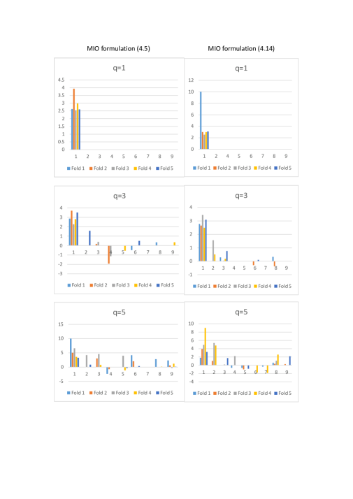
Notes: For each panel of Figure 1, the values in the horizontal axis correspond to the indices of the 9 components of the auxiliary covariate vector defined by (6.1), whereas the vertical axis displays the values of the parameter estimates. The left and right panels are based on MIO formulations (4.5) and (4.14), respectively.

We now inspect the variables selected in each of the 5 CV folds. Figure 1 summarizes the parameter estimates computed in each CV fold for the 9 auxiliary covariates specified by (6.1). From this figure, we also note that $CARS$ was selected across all $q$ cases in all CV folds. Its parameter estimate was also of a relatively large magnitude when compared to those of other selected variables. These cross-validation results further strengthen the finding that $CARS$ may be the most important predictive variable for the work-trip mode choice.

7 Concluding Remarks

In this paper, we consider the variable selection problem for predicting binary outcomes. We study the best subset selection procedure by which the covariates are chosen by maximizing the maximum score objective function subject to a constraint on the maximal number of selected covariates. We establish non-asymptotic upper and lower risk bounds for the resulting best subset maximum score binary prediction rule when the dimension of potential covariates is possibly much larger than the sample size. The derived upper and lower risk bounds are minimax rate-optimal when the maximal number of selected variables is fixed and does not increase with the sample size. For implementation, we show that the variable selection problem of this paper can be equivalently formulated as a mixed integer optimization problem, which enables computation of the exact or an approximate solution with a definite approximation error bound.

The present paper takes the maximum score approach for the binary prediction problem. There is a large body of the literature that studies maximum score estimation in various other aspects since the seminal work by Manski (1975, 1985). In the context of semiparametric binary response models, advances of the maximum score approach have been made in terms of point identification (Manski, 1988), partial identification (Manski and Tamer, 2002; Komarova, 2013; Blevins, 2015; Chen and Lee, 2015), asymptotic distribution (Kim and Pollard, 1990; Seo and Otsu, 2017), panel data (Manski, 1987; Charlier, Melenberg, and van Soest, 1995; Abrevaya, 2000), time series (Moon, 2004; Guerre and Moon, 2006; de Jong and Woutersen, 2011), dynamic network formation (Graham, 2016), nonparametrically generated regressors (Chen, Lee, and Sung, 2014), and so on. The numerical approach employed in this paper can be adapted to these contexts.

Efficient computation is particularly demanding when it is necessary to obtain maximum score estimates repeatedly many times. This difficulty naturally arises, for example, in the context of resampling (Delgado, Rodrıguez-Poo, and Wolf, 2001; Abrevaya and Huang, 2005; Lee and Pun, 2006; Patra, Seijo, and Sen, 2015) and change-point problems (Lee and Seo, 2008; Lee, Seo, and Shin, 2011). It would be an interesting future research topic to investigate numerical performance of our method (e.g. the warm-start procedure in Section 4.3) in these computation-intensive problems.

The maximum score approach has produced many offsprings: smoothed maximum score estimation (Horowitz, 1992, 2002), multinomial choice estimation (Matzkin, 1993; Fox, 2007), integrated maximum score estimation (Chen, 2010), Bayesian method (Benoit and Van den Poel, 2012), alternative estimation based on local nonlinear least squares (Blevins and Khan, 2013a, b; Khan, 2013), estimation using local polynomial smoothing (Chen and Zhang, 2015), and non-Bayesian Laplace type estimation (Jun, Pinkse, and Wan, 2015, 2017) among many others. Some of these alternative estimation methods are equipped with algorithms that are easier to compute than the maximum score estimation. It is an interesting open question how to accommodate a variable selection problem in these alternative methods. One starting point can be the work by Jiang and Tanner (2010) who considered empirical risk minimization under the $\ell_{0}$ constraint with Gibbs posterior as an alternative to maximum score prediction. It might be also interesting to consider penalized estimation with the $\ell_{0}$, $\ell_{1}$ and/or $\ell_{2}$ penalty. The maximum score approach is also closely related to the maximum utility estimation framework (Lieli and Nieto-Barthaburu, 2010; Lieli and White, 2010; Elliott and Lieli, 2013; Lieli and Springborn, 2013) for binary decision under model uncertainty. It would be interesting to generalize our results to this framework. These are also topics for future research.

Appendices

Appendix A presents proofs of all theoretical results, Appendix B gives a brief description of the branch-and-bound method for solving the mixed integer optimization problem, Appendix C reports the simulation results under the setup of DGP(ii) of Section 5, Appendix D reports an additional simulation study on the performance of adopting the warm-start strategy of Section 4.3 in solving the MIO formulations (4.5) and (4.14), and Appendix E reports additional results for the empirical example using the linear specification of covariates.

Appendix A Proofs of theoretical results

A.1 Proofs of Propositions 1, 2, and 3

Proof of Proposition 1.

By (3.22) and (3.23), we have that

$$w^{\prime}\theta^{\ast}\geq 0\Longleftrightarrow\eta(w)\geq 1/2\Longleftrightarrow b^{\ast}(w)=1.$$ (A.1)

Since the functional $\widetilde{S}(b^{\ast})$ is maximized at $b=b^{\ast}$ and, by Condition 1, this maximum is unique, we have that

$$b^{\ast}\in\mathcal{B}_{q}\Longleftrightarrow b^{\ast}=b_{\theta_{0}}.$$ (A.2)

By (1.1), we have that

$$b_{\theta_{0}}(w)=1\Longleftrightarrow w^{\prime}\theta_{0}\geq 0.$$ (A.3)

Thus it follows from (A.1), (A.2) and (A.3) that $b^{\ast}\in\mathcal{B}_{q}$ if and only if $W^{\prime}\theta_{0}$ and $W^{\prime}\theta^{\ast}$ have the same sign with probability 1.    

Proof of Proposition 2.

Let $G_{w}(t)\equiv P\left(\xi\leq t|W=w\right)$. By (3.22) and (3.23), we have that $\eta(w)=G_{w}(w^{\prime}\theta^{\ast})$ and $G_{w}(0)=1/2$. By condition (ii) of Proposition 2, it hence follows that, if $w^{\prime}\theta^{\ast}\geq\kappa_{1}$, then

$$\eta(w)\geq G_{w}(\kappa_{1})\geq 1/2+\kappa_{1}\kappa_{2}.$$

On the other hand, by similar arguments, we have that, if $w^{\prime}\theta^{\ast}\leq-\kappa_{1}$, then

$$\eta(w)\leq G_{w}(-\kappa_{1})\leq 1/2-\kappa_{1}\kappa_{2}.$$

Combing these results and using condition (i) of Proposition 2, we thus deduce that condition (3.24) holds with $h=2\kappa_{1}\kappa_{2}$.    

Proof of Proposition 3.

Consider any two vectors $\theta=\left(\alpha,\beta,\gamma\right),$ $\widetilde{\theta}=(\widetilde{\alpha},\widetilde{\beta},\widetilde{\gamma})\in\{-1,1\}\times\Theta_{q}$ such that $\alpha=\widetilde{\alpha}$ and $\beta=\widetilde{\beta}$. We now prove this proposition for the case $\alpha=\widetilde{\alpha}=1$. The other case $\alpha=\widetilde{\alpha}=-1$ can be proved using identical arguments and hence is omitted.

Assume $\alpha=\widetilde{\alpha}=1.$ Note that

$$\left\|b_{\theta}-b_{\widetilde{\theta}}\right\|_{1}$$

$$= P\left(-\widetilde{X}\beta-Z^{\prime}\gamma\leq X_{0}<-\widetilde{X}\widetilde{\beta}-Z^{\prime}\widetilde{\gamma}\right)+P\left(-\widetilde{X}\beta-Z^{\prime}\gamma>X_{0}\geq-\widetilde{X}\widetilde{\beta}-Z^{\prime}\widetilde{\gamma}\right)$$

$$= E\left[P\left(-\widetilde{X}\beta-Z^{\prime}\gamma\leq X_{0}<-\widetilde{X}\widetilde{\beta}-Z^{\prime}\widetilde{\gamma}|\widetilde{X},Z\right)1\left\{Z^{\prime}\gamma\geq Z^{\prime}\widetilde{\gamma}\right\}\right]$$

$$+E\left[P\left(-\widetilde{X}\beta-Z^{\prime}\gamma>X_{0}\geq-\widetilde{X}\widetilde{\beta}-Z^{\prime}\widetilde{\gamma}|\widetilde{X},Z\right)1\left\{Z^{\prime}\gamma\leq Z^{\prime}\widetilde{\gamma}\right\}\right].$$

By Condition (a) of Proposition 3, we hence have that

$$E\left[\left|Z^{\prime}\left(\gamma-\widetilde{\gamma}\right)\right|\right]L_{1}^{-1}\leq\left\|b_{\theta}-b_{\widetilde{\theta}}\right\|_{1}\leq E\left[\left|Z^{\prime}\left(\gamma-\widetilde{\gamma}\right)\right|\right]L_{1}.$$ (A.4)

Let $J\equiv\{j\in\left\{1,...,p\right\}:\gamma_{j}\neq\widetilde{\gamma}_{j}\}$. Since $\left\|\gamma\right\|_{0}\leq q$ and $\left\|\widetilde{\gamma}\right\|_{0}\leq q$, we have that $\left|J\right|\leq 2q$. Therefore, $Z^{\prime}\left(\gamma-\widetilde{\gamma}\right)=Z_{J}^{\prime}\delta_{J}$ where $Z_{J}$ denotes the subvector of $Z\equiv(Z^{(1)},\ldots,Z^{(p)})^{\prime}$ formed by keeping only those elements $Z^{(j)}$ with $j\in J$ and $\delta_{J}$ denotes the subvector of $\gamma-\widetilde{\gamma}$ formed by keeping only those elements $(\gamma_{j}-\widetilde{\gamma}_{j})$ with $j\in J$.

By Condition (b) and Cauchy-Schwarz inequality, we have that with probability 1,

$$\left|Z_{J}^{\prime}\delta_{J}\right|\leq L_{2}\left\|\delta_{J}\right\|_{E}$$ (A.5)

and hence

$$\frac{\delta_{J}^{\prime}Z_{J}Z_{J}^{\prime}\delta_{J}}{L_{2}^{2}\left\|\delta_{J}\right\|_{E}^{2}}\leq\frac{\left|Z_{J}^{\prime}\delta_{J}\right|}{L_{2}\left\|\delta_{J}\right\|_{E}}\leq 1.$$ (A.6)

Using (A.6) and the assumption that the smallest eigenvalue of $E\left(Z_{J}Z_{J}^{\prime}\right)$ is bounded below by $L_{3}$, we thus have that

$$E\left[\left|Z_{J}^{\prime}\delta_{J}\right|\right]\geq L_{2}^{-1}L_{3}\left\|\delta_{J}\right\|_{E}.$$ (A.7)

Noting that $\left\|\delta_{J}\right\|_{E}=\left\|\theta-\widetilde{\theta}\right\|_{E}$ and combining (A.4), (A.5) and (A.7), we conclude that condition (3.25) holds with $c_{u}=L_{1}L_{2}$ and $c_{l}=(L_{1}L_{2})^{-1}L_{3}$.    

A.2 Proof of Theorem 1

Recall the notation $\theta=(\alpha,\beta,\gamma)$. Let

$$G_{n}(\theta)\equiv\sqrt{n}\left[S_{n}(\theta)-S(\theta)\right].$$

We first present the following lemma, which will be used to prove Theorem 1.

Lemma 1.

For $t>0$, there is a universal constant $D$ such that

$$P\left(\sup\limits_{\theta\in\{-1,1\}\times\Theta_{q}}\left|G_{n}(\theta)\right|>t\right)\leq 2\binom{p}{q}\left(\frac{Dt}{\sqrt{4s+4}}\right)^{4s+4}e^{-2t^{2}}.$$

Proof.

Let $m$ be a subset of the index set $\left\{1,...,p\right\}$ such that $m$ contains only $q$ elements. Let $\mathcal{M}$ be the collection of all such subsets. Note that $\left|\mathcal{M}\right|=\binom{p}{q}$. For $m\in\mathcal{M}$, let

$$\Gamma_{m}\equiv\{\left(\beta,\gamma\right)\in\Theta:\gamma_{j}=0\text{ for }j\notin m\}.$$

For any $t>0$, we have that

$$P\left(\sup\limits_{\theta\in\{-1,1\}\times\Theta_{q}}\left|G_{n}(\theta)\right|>t\right) \leq\sum_{m\in\mathcal{M}}P\left(\sup\limits_{\left(\beta,\gamma\right)\in\Gamma_{m}}\left|G_{n}(1,\beta,\gamma)\right|>t\right)$$

$$+\sum_{m\in\mathcal{M}}P\left(\sup\limits_{\left(\beta,\gamma\right)\in\Gamma_{m}}\left|G_{n}(-1,\beta,\gamma)\right|>t\right).$$ (A.8)

To complete the proof, it remains to derive the bounds on the tail probability terms on the right hand side of the inequality above.

Consider the function $f_{\theta}:\{0,1\}\times\mathcal{W\mapsto}\{0,1\}$ defined by

$$f_{\theta}(y,w) \equiv 1\left\{y=b_{\theta}(w)\right\}$$

$$=1-y+\left(2y-1\right)b_{\theta}.$$

For $m\in\mathcal{M}$, let

$$\digamma_{m}^{+} \equiv\{f_{\theta}:\theta\in\{1\}\times\Gamma_{m}\},$$

$$\digamma_{m}^{-} \equiv\{f_{\theta}:\theta\in\{-1\}\times\Gamma_{m}\}.$$

For each $m\in\mathcal{M}$, by Lemmas 9.6 and 9.9 of Kosorok (2008), the class of functions $\digamma_{m}^{+}$  and $\digamma_{m}^{-}$ are both $VC$ classes of functions with $VC$ indices $V(\digamma_{m}^{+})$ and $V(\digamma_{m}^{-})$ satisfying that

$$V(\digamma_{m}^{+})=V(\digamma_{m}^{-})\leq 2s+3.$$

For two measurable functions $f$ and $g$ and a given probability measure $Q$, define the (semi-) metric

$$d_{Q}(f,g)\equiv\sqrt{\int\left(f-g\right)^{2}dQ}.$$

By Theorem 9.3 of Kosorok (2008), we have that, for some universal constant $K>1$ and $0<\epsilon<1$,

$$\sup\nolimits_{Q}N\left(\epsilon,\digamma_{m}^{+},d_{Q}\right)\vee\sup\nolimits_{Q}N\left(\epsilon,\digamma_{m}^{-},d_{Q}\right)$$

$$\leq K\left(2s+3\right)\left(16e\right)^{2s+3}\left(\epsilon\right)^{-4(s+1)}$$

$$\leq\left(\frac{\Lambda(s)}{\epsilon}\right)^{4s+4},$$

where

$$\Lambda(s)\equiv\left[K\left(2s+3\right)\left(16e\right)^{2s+3}\right]^{\frac{1}{4s+4}}$$

and, for a given class of functions $\digamma$, $N\left(\epsilon,\digamma,d_{Q}\right)$ denotes the minimal number of open balls (defined under the metric $d_{Q}$) of radius $\epsilon$ required to cover $\digamma$.

Observe that

$$\Lambda(s)\leq 16Ke\left(2s+3\right)^{\frac{1}{4s+4}}\leq 32Ke,$$ (A.9)

where the second inequality follows from the fact that $i\leq 2^{i}$ for all integer $i$.

Using (A.9), we can apply Theorem 1.3 of Talagrand (1994) to deduce that, for $t>0$, there is a universal constant $D$ such that

$$P\left(\sup\limits_{\left(\beta,\gamma\right)\in\Gamma_{m}}\left|G_{n}(1,\beta,\gamma)\right|>t\right)\vee P\left(\sup\limits_{\left(\beta,\gamma\right)\in\Gamma_{m}}\left|G_{n}(-1,\beta,\gamma)\right|>t\right)$$

$$\leq\left(\frac{Dt}{\sqrt{4s+4}}\right)^{4s+4}e^{-2t^{2}}.$$ (A.10)

Lemma 1 hence follows by combining inequalities (A.8) and (A.10).    

We now prove Theorem 1.

Proof of Theorem 1.

By Lemma 1 and using the fact that $\binom{p}{q}\leq p^{q},$ we have that, for some universal constant $D$ and for $t>0$,

$$P\left(\sup\limits_{\theta\in\{-1,1\}\times\Theta_{q}}\left|G_{n}(\theta)\right|>t\right)\leq 2p^{q}\left(\frac{Dt}{\sqrt{4s+4}}\right)^{4s+4}e^{-2t^{2}}.$$ (A.11)

For $t\geq D$ and $s\geq 1$, the right hand side term of (A.11) can be further bounded above by

$$p^{s}t^{8s+8}2^{-6s-5}e^{-2t^{2}}=e^{\lambda(s,p,t)},$$ (A.12)

where

$$\lambda(s,p,t)\equiv-2t^{2}+\left(8s+8\right)\ln t+s\ln p-\left(6s+5\right)\ln 2.$$

For $\sigma>0$, let

$$t=\sqrt{M_{\sigma}r_{n}}$$ (A.13)

where

$$M_{\sigma}\equiv\left(1+\sigma/2\right)\vee D^{2}.$$ (A.14)

Note that $t\geq D$ by (A.13) and (A.14). Thus with the $t$ value specified by (A.13), we have that

$$\lambda(s,p,t)\leq\left(-2M_{\sigma}+1\right)r_{n}+\left(4s+4\right)\ln\left(M_{\sigma}r_{n}\right)-\left(6s+5\right)\ln 2\leq-\sigma r_{n}$$ (A.15)

where the second inequality follows from (A.14) and (3.6).

It is straightforward to see that

$$U_{n} =\sup\limits_{\theta\in\{-1,1\}\times\Theta_{q}}\text{ }S(\theta)-S(\widehat{\theta})$$

$$\leq\sup\limits_{\theta\in\{-1,1\}\times\Theta_{q}}\left|S_{n}(\theta)-S(\theta)\right|+\sup\limits_{\theta\in\{-1,1\}\times\Theta_{q}}S_{n}(\theta)-S(\widehat{\theta})$$

$$\leq\sup\limits_{\theta\in\{-1,1\}\times\Theta_{q}}\left|S_{n}(\theta)-S(\theta)\right|+S_{n}(\widehat{\theta})-S(\widehat{\theta})$$

$$\leq 2\sup\limits_{\theta\in\{-1,1\}\times\Theta_{q}}\left|S_{n}(\theta)-S(\theta)\right|.$$

Hence, we have that

$$P\left(U_{n}>2\sqrt{\frac{M_{\sigma}r_{n}}{n}}\right)\leq P\left(\sup\limits_{\theta\in\{-1,1\}\times\Theta_{q}}\left|G_{n}(\theta)\right|>\sqrt{M_{\sigma}r_{n}}\right).$$ (A.16)

Therefore, Theorem 1 follows by putting together the results of (A.11), (A.12) and (A.15) and then concluding that the right hand side term of (A.16) is bounded above by $e^{-\sigma r_{n}}$ under condition (3.6).    

A.3 Proof of Theorem 2

We first introduce some notation which will be used in the proof Theorem 2. Let $\mathcal{A}$ be a collection of subsets of $\mathcal{W}$. For any subset $S\subset\mathcal{W}$, let $T_{\mathcal{A}}(S)$ denote the trace of $\mathcal{A}$ on $S$ defined by

$$T_{\mathcal{A}}(S)=\left\{A\cap S:A\in\mathcal{A}\right\}.$$

If $\mathcal{A=\cup}_{j\in J}\mathcal{A}_{j}$, then we have

$$T_{\mathcal{A}}(S)\subset\mathcal{\cup}_{j\in J}T_{\mathcal{A}_{j}}(S)\text{ for }S\subset\mathcal{W}\text{.}$$ (A.17)

We now prove Theorem 2.

Proof of Theorem 2.

By (1.1), (3.1), (3.2) and (3.15), we have that

$$S(\widehat{\theta})=\widetilde{S}\left(b_{\widehat{\theta}}\right)\text{ and }S_{q}^{\ast}=\sup\nolimits_{b\in\mathcal{B}_{q}}\widetilde{S}\left(b\right).$$ (A.18)

Theorem 2 is an application of Theorem 2 of Massart and Nédélec (2006) to the binary prediction problem. Massart and Nédélec (2006, Section 2.4) showed how to apply their Theorem 2 to derive the risk upper bound for the empirical risk minimizer. Using their derived results (Massart and Nédélec (2006, p. 2340)) in their Theorem 2 for our setup, we conclude that, under Condition 1, there are universal constants $K$ and $K^{\prime}$ such that

$$\begin{split}&E\left[\widetilde{S}\left(b^{\ast}\right)-\widetilde{S}\left(b_{\widehat{\theta}}\right)\right]\\ &\leq 2\left[\widetilde{S}\left(b^{\ast}\right)-\sup\nolimits_{b\in\mathcal{B}_{q}}\widetilde{S}\left(b\right)\right]\\ &+K^{\prime}\left[\left(\frac{K^{2}\left(1\vee E(H_{\mathcal{A}})\right)}{nh}\right)^{\vartheta/\left(2\vartheta-1\right)}\wedge\sqrt{\frac{K^{2}\left(1\vee E(H_{\mathcal{A}})\right)}{n}}\right],\end{split}$$ (A.19)

where

$$\mathcal{A} \mathcal{\equiv}\{A_{\theta}:\theta\in\{-1,1\}\times\Theta_{q}\},$$

$$A_{\theta} \equiv\{w\in\mathcal{W}:w^{\prime}\theta\geq 0\},$$

and $H_{\mathcal{A}}$ is the random combinatorial entropy of $\mathcal{A}$ defined by

$$H_{\mathcal{A}}=\ln\left(\left|T_{\mathcal{A}}(\left\{W_{1},W_{2},...,W_{n}\right\})\right|\right),$$

where

$$T_{\mathcal{A}}(\left\{W_{1},W_{2},...,W_{n}\right\})=\left\{A\cap\left\{W_{1},W_{2},...,W_{n}\right\}:A\in\mathcal{A}\right\}$$ (A.20)

is the trace of $\mathcal{A}$ on the covariate data $\left\{W_{1},W_{2},...,W_{n}\right\}$.

Using (3.3) and (A.18), it follows that

$$U_{n} = \sup\nolimits_{b\in\mathcal{B}_{q}}\widetilde{S}\left(b\right)-\widetilde{S}\left(b_{\widehat{\theta}}\right)$$ (A.21)

$$= \left[\sup\nolimits_{b\in\mathcal{B}_{q}}\widetilde{S}\left(b\right)-\widetilde{S}\left(b^{\ast}\right)\right]+\left[\widetilde{S}\left(b^{\ast}\right)-\widetilde{S}\left(b_{\widehat{\theta}}\right)\right].$$

To complete the proof, it thus remains to derive an upper bound on the term $E(H_{\mathcal{A}})$.

Let $m$ be a subset of the index set $\left\{1,...,p\right\}$ such that $m$ contains only $q$ elements. Let $\mathcal{M}$ be the collection of all such subsets. Note that $\left|\mathcal{M}\right|=\binom{p}{q}$. For $m\in\mathcal{M}$, let

$$\mathcal{A}_{m}^{+} \mathcal{\equiv}\{A_{\theta}:\theta\in\{1\}\times\Gamma_{m}\},$$

$$\mathcal{A}_{m}^{-} \mathcal{\equiv}\{A_{\theta}:\theta\in\{-1\}\times\Gamma_{m}\},$$

$$\Gamma_{m} \equiv\{\left(\beta,\gamma\right)\in\Theta:\gamma_{j}=0\text{ for }j\notin m\}\text{.}$$

It is immediate to see that

$$\mathcal{A=\cup}_{m\in\mathcal{M}}\left(\mathcal{A}_{m}^{+}\cup\mathcal{A}_{m}^{-}\right).$$ (A.22)

For each $m\in\mathcal{M}$, by Lemmas 9.6 and 9.9 of Kosorok (2008), the family of sets $\mathcal{A}_{m}^{+}$  and $\mathcal{A}_{m}^{-}$ are both $VC$ classes of sets with $VC$ indices $V(\mathcal{A}_{m}^{+})$ and $V(\mathcal{A}_{m}^{-})$ satisfying that

$$V(\mathcal{A}_{m}^{+})=V(\mathcal{A}_{m}^{-})\leq s+2.$$

Hence by Corollary 1.3 of Lugosi (2002), we have that

$$\left|T_{\mathcal{A}_{m}^{+}}(\left\{W_{1},W_{2},...,W_{n}\right\})\right|\vee\left|T_{\mathcal{A}_{m}^{-}}(\left\{W_{1},W_{2},...,W_{n}\right\})\right|\leq(n+1)^{s+1}.$$ (A.23)

By (A.17), (A.22) and (A.23), we thus have that

$$H_{\mathcal{A}} \leq\ln 2+\ln\binom{p}{q}+\left(s+1\right)\ln\left(n+1\right)$$

$$\leq\ln 2+q\ln p+\left(s+1\right)\ln\left(n+1\right).$$ (A.24)

Theorem 2 therefore follows by combining the results (A.19), (A.21) and (A.24).    

A.4 Proof of Theorem 3

Proof of Theorem 3.

Define

$$R_{n}(h,\mathcal{B}_{q})=\inf_{\widehat{b}\in\mathcal{B}_{q}}\sup_{F\in\mathcal{P}(h,\mathcal{B}_{q})}E_{F}\left[\widetilde{S}\left(b^{\ast}\right)-\widetilde{S}(\widehat{b})\right]$$

where the infimum is taken over the set of all binary predictors in $\mathcal{B}_{q}$ that are constructed based on the data $\left(Y_{i},W_{i}\right)_{i=1}^{n}$. By (3.2), it follows that $S_{q}^{\ast}=\widetilde{S}\left(b^{\ast}\right)$ under $F\in\mathcal{P}(h,\mathcal{B}_{q})$. Thus Theorem 3 is proved once we show that

$$R_{n}(h,\mathcal{B}_{q})\geq\frac{\phi qc_{l}\left(1-\phi\right)\left(1-h\right)}{32nhc_{u}}\ln\left(\frac{p-q}{q/2}\right).$$ (A.25)

For any indicator function $b\in\mathcal{B}_{q}$, let

$$\eta_{b}(w)\equiv\left[1+\left(2b(w)-1\right)h\right]/2\text{ for }w\in\mathcal{W}.$$

Let $F_{b}$ denote the joint distribution of $\left(Y,W\right)$ such that under $F_{b}$, the distribution of $W$ satisfies condition (3.25), and $Y$ conditional on $W=w$ follows a Bernoulli distribution with parameter $\eta_{b}(w)$ for every $w\in\mathcal{W}$. By the same arguments as those in the proof of Theorem 6 of Massart and Nédélec (2006, p. 2355), we can deduce that, for any finite subset $\mathcal{C}$ of $\mathcal{B}_{q}$,

$$\left\{F_{b}:b\in\mathcal{C}\right\}\subset\mathcal{P}(h,\mathcal{B}_{q})$$ (A.26)

and

$$R_{n}(h,\mathcal{B}_{q})\geq\frac{h}{2}\inf_{\widehat{b}\in\mathcal{C}}\sup_{b\in\mathcal{C}}E_{F_{b}}\left[\left\|b-\widehat{b}\right\|_{1}\right].$$ (A.27)

Consider the set

$$\mathcal{H}\equiv\left\{\gamma\in\left\{-1,0,1\right\}^{p}:\left\|\gamma\right\|_{0}=q\right\}.$$

By Lemma 4 of Raskutti, Wainwright, and Yu (2011), we have that, for $p,q$ even and $q<2p/3$, there is a subset $\mathcal{A\subset H}$ with cardinality

$$\left|\mathcal{A}\right|\geq\left(\frac{p-q}{q/2}\right)^{q/2}$$ (A.28)

such that

$$\left\|\gamma-\gamma^{\prime}\right\|_{0}\geq q/2\text{ for all }\gamma,\gamma^{\prime}\in\mathcal{A}\text{ and }\gamma\neq\gamma^{\prime}.$$ (A.29)

Let

$$\mathcal{D\equiv}\{1\}\times\{\underline{0}\}\times\epsilon_{n}\mathcal{A}$$ (A.30)

where $\underline{0}=(0,...,0)$ denotes the $k$-dimensional vector of which all elements take value $0$, and $\epsilon_{n}>0$ is a given sequence that will be chosen later. Note that, for any $\theta,\widetilde{\theta}\in\mathcal{D}$,

$$\epsilon_{n}^{2}\left\|\theta-\widetilde{\theta}\right\|_{0}\leq\left\|\theta-\widetilde{\theta}\right\|_{E}^{2}\leq 4\epsilon_{n}^{2}\left\|\theta-\widetilde{\theta}\right\|_{0}.$$ (A.31)

Now take

$$\mathcal{C=}\left\{b_{\theta}\in\mathcal{B}_{q}:\theta\in\mathcal{D}\right\}.$$ (A.32)

We then have that

$$R_{n}(h,\mathcal{B}_{q}) \geq\frac{h}{2}\inf_{\widehat{\theta}\in\mathcal{D}}\sup_{\theta\in\mathcal{D}}E_{F_{b_{\theta}}}\left[\left\|b_{\theta}-b_{\widehat{\theta}}\right\|_{1}\right]$$ (A.33)

$$\geq\frac{hc_{l}}{2}\inf_{\widehat{\theta}\in\mathcal{D}}\sup_{\theta\in\mathcal{D}}E_{F_{b_{\theta}}}\left[\left\|\theta-\widehat{\theta}\right\|_{E}\right]$$ (A.34)

$$\geq\frac{hc_{l}\epsilon_{n}}{2}\inf_{\widehat{\theta}\in\mathcal{D}}\sup_{\theta\in\mathcal{D}}E_{F_{b_{\theta}}}\left[\sqrt{\left\|\theta-\widehat{\theta}\right\|_{0}}\right]$$ (A.35)

$$\geq\frac{hc_{l}\epsilon_{n}\sqrt{q}}{2\sqrt{2}}\inf_{\widehat{\theta}\in\mathcal{D}}\sup_{\theta\in\mathcal{D}}P_{F_{b_{\theta}}}\left(\widehat{\theta}\neq\theta\right)$$ (A.36)

$$\geq\frac{hc_{l}\epsilon_{n}\sqrt{q}}{2\sqrt{2}}\inf_{\widehat{\theta}\in\mathcal{D}}\left[1-\inf_{\theta\in\mathcal{D}}P_{F_{b_{\theta}}}\left(\widehat{\theta}=\theta\right)\right],$$ (A.37)

where the infimum in (A.33) is taken over the set of all estimators $\widehat{\theta}$ taking values in $\mathcal{D}$; (A.34) follows from (A.26), (A.32) and (3.25); (A.35) follows from (A.31); (A.36) follows from (A.29).

By Lemma 8 of Massart and Nédélec (2006), we have that, for a given point $\widetilde{\theta}\in\mathcal{D}$,

$$\inf_{\theta\in\mathcal{D}}P_{F_{b_{\theta}}}\left(\widehat{\theta}=\theta\right)\leq\phi\vee\frac{\overline{\mathcal{K}}}{\ln\left(\left|\mathcal{D}\right|\right)},$$ (A.38)

where

$$\overline{\mathcal{K}}=\frac{n}{\left|\mathcal{D}\right|-1}\sum_{\theta\in\mathcal{D},\theta\neq\widetilde{\theta}}\mathcal{K}\left(F_{b_{\theta}},F_{b_{\widetilde{\theta}}}\right),$$

and $\mathcal{K}\left(F_{b_{\theta}},F_{b_{\widetilde{\theta}}}\right)$ is the Kullback-Leibler information between $F_{b_{\theta}}$ and $F_{b_{\widetilde{\theta}}}$. For $\widetilde{\theta},\theta\in\mathcal{D}$ and $\theta\neq\widetilde{\theta}$, using Lemma 7 of Massart and Nédélec (2006), we have that, for $h<1$,

$$\mathcal{K}\left(F_{b_{\theta}},F_{b_{\widetilde{\theta}}}\right) =h\ln\left(\frac{1+h}{1-h}\right)\left\|b_{\theta}-b_{\widetilde{\theta}}\right\|_{1}$$

$$\leq\frac{2c_{u}h^{2}}{1-h}\left\|\theta-\widetilde{\theta}\right\|_{E}$$

$$\leq\frac{4c_{u}h^{2}\epsilon_{n}}{1-h}\sqrt{\left\|\theta-\widetilde{\theta}\right\|_{0}}$$

$$\leq\frac{4c_{u}h^{2}\epsilon_{n}\sqrt{2q}}{1-h},$$

where the last inequality follows since $\left\|\theta-\widetilde{\theta}\right\|_{0}\leq 2q$ for all $\widetilde{\theta},\theta\in\mathcal{D}$. Hence, we have that

$$\overline{\mathcal{K}}\leq\frac{4nc_{u}h^{2}\epsilon_{n}\sqrt{2q}}{1-h}.$$ (A.39)

Putting together (A.37), (A.38) and (A.39), we have that

$$R_{n}(h,\mathcal{B}_{q})\geq\frac{h\epsilon_{n}c_{l}\sqrt{q}}{2\sqrt{2}}\left(1-\phi\right)$$ (A.40)

provided that

$$\frac{4nc_{u}h^{2}\epsilon_{n}\sqrt{2q}}{\left(1-h\right)\ln\left(\left|\mathcal{D}\right|\right)}\leq\phi.$$ (A.41)

By (A.28) and (A.30), condition (A.41) holds whenever

$$\frac{8nc_{u}h^{2}\epsilon_{n}\sqrt{2q}}{\left(1-h\right)q\ln\left(\frac{p-q}{q/2}\right)}\leq\phi.$$ (A.42)

By (3.26), (A.30) and (A.32), we have that $\epsilon_{n}\leq\kappa.$ Therefore, we can get the result (A.25) by setting

$$\epsilon_{n}=\frac{\phi\sqrt{q}\left(1-h\right)\ln\left(\frac{p-q}{q/2}\right)}{8nc_{u}h^{2}\sqrt{2}}$$

provided that this choice of $\epsilon_{n}$ also satisfies that $\epsilon_{n}\leq\kappa$, which can be easily seen to hold under the condition (3.28) for the lower bound on the value of $h$.    

Appendix B The Branch-and-Bound Method for Solving MIO Problems

For completeness of the paper and for readers who are unfamiliar with MIO, we will present briefly the branch-and-bound method for solving the MIO problem. For further details, see, e.g., Conforti, Cornuéjols, and Zambelli (2014) for a recent and comprehensive study on the MIO theory and solution methods.

We take the formulation (4.5) as an expositional example and explain how the branch-and-bound method can be used to solve this MIO problem. The maximization problem (4.5) consists of $n+p$ binary control variables. Let $v=(d_{1},...,d_{n},e_{1},...,e_{p})$ denote the vector that collects all these binary controls. Let $\widetilde{S}_{n}\left(\beta,\gamma,v\right)$ denote the objective function of (4.5). We may maximize $\widetilde{S}_{n}$ over $v$ by enumerating all possible values of $v$, which amounts to exhaustively searching over a binary tree that has $2^{n+p}$ leaf nodes. This naive method is inefficient and becomes practically infeasible for large scale problems. The branch-and-bound method improves the search efficiency by avoid visiting those tree nodes which can be fathomed not to constitute the optimum.

Let $\Gamma_{0}$ denote the space of the controls $\left(\beta,\gamma,v\right)$ defined by all the constraints stated in the MIO problem (4.5). Let $\overline{\Gamma}_{0}$ be an enlargement of $\Gamma_{0}$, which is defined analogously to $\Gamma_{0}$ with the dichotomization constraints $v\in\{0,1\}^{n+p}$ being replaced by the constraints $v\in[0,1]^{n+p}$. Optimizing the objective function $\widetilde{S}_{n}$ over $\left(\beta,\gamma,v\right)\in\overline{\Gamma}_{0}$ reduces to a simple linear programming (LP) problem. Clearly, the maximized objective value of this LP relaxation problem forms an upper bound on the function $\widetilde{S}_{n}\left(\beta,\gamma,v\right)$ defined on the original domain $\Gamma_{0}$. Moreover, if the solution for $v$ in the LP relaxation problem turns out to be a vector of binary values, we can deduce that the LP relaxation solution for $\left(\beta,\gamma,v\right)$ is also the solution to the MIO problem (4.5).

When the LP relaxation solution for $v$ contains fractional-valued elements, we choose a fractional-valued element $v_{j}$ and then construct the two LP sub-problems, denoted as $LP_{1}$ and $LP_{1}^{\prime}$, which correspond to maximizing $\widetilde{S}_{n}\left(\beta,\gamma,v\right)$ over the subspaces $\overline{\Gamma}_{1}\equiv$ $\overline{\Gamma}_{0}\cap\left\{\left(\beta,\gamma,v\right):v_{j}=0\right\}$ and $\overline{\Gamma}_{1}^{\prime}\equiv$ $\overline{\Gamma}_{0}\cap\left\{\left(\beta,\gamma,v\right):v_{j}=1\right\}$, respectively. Consider the problem $LP_{1}$ and note that the treatment of $LP_{1}^{\prime}$ is similar. There are four possible cases for $LP_{1}$: (i) $\overline{\Gamma}_{1}$ is empty and hence $LP_{1}$ is infeasible. (ii) $\overline{\Gamma}_{1}$ is non-empty and the maximized objective value of $LP_{1}$ is not larger than the best known lower bound on the objective value of (4.5). (iii) $\overline{\Gamma}_{1}$ is non-empty, the maximized objective value of $LP_{1}$ is larger than the best known lower bound on the objective value of (4.5), and the solution for $v$ of $LP_{1}$ is in $\{0,1\}^{n+p}$. (iv) $\overline{\Gamma}_{1}$ is non-empty, the maximized objective value of $LP_{1}$ is larger than the best known lower bound on the objective value of (4.5), and the solution for $v$ of $LP_{1}$ contains fractional-valued elements.

For cases (i) and (ii), we can bypass further sub-problems of $LP_{1}$ since these will not yield a solution to the MIO problem (4.5). In other words, all nodes of the binary search tree along the branch implied by $LP_{1}$ can be pruned and need not be further considered. For case (iii), we can update the best known feasible solution to the MIO problem (4.5) as the optimal solution to the problem $LP_{1}$. For case (iv), the sub-domain $\Gamma_{0}\cap\left\{\left(\beta,\gamma,v\right):v_{j}=0\right\}$ may still contain an optimal solution. Therefore, in case (iv), we branch on a fraction-valued component of the $LP_{1}$ solution for $v$ to create further two sub-problems and then repeat this process as described above.

Appendix C Simulation Results for the DGP(ii) Design

In this part of the appendix, we report the simulation results under the setup of DGP(ii) of Section 5. Table 7 gives the MIO computation time statistics for solving the PRESCIENCE($q$) problem under DGP(ii). Compared to the results of Table 1, the PRESCIENCE problem appeared to be more computationally difficult for the high dimensional setup in the DGP(ii) design where the maximum computation time could exceed 2.5 hours. However, the mean and median computation time remained well capped below 6 minutes across all cases in Table 7. In fact, the case of the MIO computation lasting over one hour appeared in only 3 out of the 100 repetitions for the PRESCIENCE(3) simulations in the setup of $p=60$.

Table 7: PRESCIENCE computation time (CPU seconds) under DGP(ii)

	$p=10$			$p=60$
$q$	1	2	3	1	2	3
mean	0.39	1.55	0.73	3.47	68.53	350.4
min	0.05	0.04	0.03	0.21	0.03	0.04
median	0.40	0.76	0.38	2.77	23.07	50.13
max	1.02	20.34	9.97	16.56	417.2	8552

Table 8: Comparison of prediction methods under DGP(ii) with $p=10$

method	PRESCIENCE($q$)			PRE_CV	logit_lasso			probit_lasso
	${\small q=1}$	${\small q=2}$	${\small q=3}$		${\small\lambda}_{\min}$	${\small\lambda}_{1se}$	${\small\lambda}_{2se}$	${\small\lambda}_{\min}$	${\small\lambda}_{1se}$	${\small\lambda}_{2se}$
${\small Corr\_sel}$	0.86	0.95	0.95	0.91	0.91	0.6	0.27	0.88	0.55	0.28
${\small Orac\_sel}$	0.86	0.01	0	0.53	0.09	0.3	0.16	0.09	0.3	0.16
${\small Num\_irrel}$	0.14	1.04	2.02	0.67	2.93	0.62	0.26	2.49	0.51	0.26
${\small in\_Score}$	0.834	0.871	0.894	0.860	0.787	0.710	0.630	0.776	0.695	0.627
${\small in\_RS}$	1.095	1.144	1.175	1.131	1.031	0.930	0.825	1.016	0.910	0.822
${\small out\_Score}$	0.724	0.711	0.696	0.716	0.673	0.614	0.553	0.668	0.606	0.552
${\small out\_RS}$	0.948	0.930	0.910	0.937	0.881	0.804	0.724	0.874	0.794	0.723

Table 9: Comparison of prediction methods under DGP(ii) with $p=60$

method	PRESCIENCE($q$)			PRE_CV	logit_lasso			probit_lasso
	${\small q=1}$	${\small q=2}$	${\small q=3}$		${\small\lambda}_{\min}$	${\small\lambda}_{1se}$	${\small\lambda}_{2se}$	${\small\lambda}_{\min}$	${\small\lambda}_{1se}$	${\small\lambda}_{2se}$
${\small Corr\_sel}$	0.76	0.82	0.88	0.82	0.64	0.45	0.29	0.63	0.43	0.28
${\small Orac\_sel}$	0.76	0	0	0.41	0	0.13	0.16	0	0.11	0.15
${\small Num\_irrel}$	0.24	1.18	2.12	0.88	4.53	1.17	0.47	4.17	1.06	0.44
${\small in\_Score}$	0.842	0.894	0.927	0.880	0.766	0.680	0.629	0.759	0.673	0.626
${\small in\_RS}$	1.103	1.171	1.216	1.153	1.000	0.887	0.821	0.990	0.878	0.817
${\small out\_Score}$	0.713	0.693	0.673	0.700	0.608	0.575	0.540	0.608	0.571	0.539
${\small out\_RS}$	0.934	0.907	0.881	0.917	0.797	0.753	0.708	0.796	0.748	0.706

We compare in Tables 8 and 9 the predictive and variable selection performance results for the various prediction methods given in (5.2). For the penalized MLE approaches, the logit_lasso and probit_lasso implemented with $\lambda_{\min}$ performed better in terms of predictive performance than those implemented with $\lambda_{1se}$ or $\lambda_{2se}$. Yet, the PRE_CV approach still had the best overall performance among all the prediction approaches in Tables 8 and 9. We also note that the PRE_CV approach could outperform the logit_lasso and probit_lasso approaches by a large margin in both the in-sample and out-of-sample predictive performances in the high dimensional variable selection setup.

It is well known in the binary prediction literature (see e.g. Elliott and Lieli, 2013) that the optimal prediction rule in terms of score maximization does not hinge on knowing the true distribution of $Y$ given $W$, and binary prediction based on the MLE approach with a misspecified likelihood can yield poor predictive performance. For the DGP(ii) design, the binary response probability $P(Y=1|W)$ depends on the index $\left[\sigma(W)\right]^{-1}W^{\prime}\theta$, which is nonlinear in the variables $V_{1}$ and $V_{2}$, such that the logit and probit likelihoods with an index linear in $W$ are misspecified. We approximated this nonlinearity by using covariates that consisted of cubic polynomial terms in $\left(V_{1},V_{2}\right)$. Specifically, we replaced the last 7 variables of the original auxiliary covariates $\left(V_{2},...,V_{p+1}\right)$ by the vector

$$(V_{1}^{2},V_{2}^{2},V_{1}^{3},V_{2}^{3},V_{1}V_{2},V_{1}V_{2}^{2},V_{1}^{2}V_{2}),$$

where each nonlinear covariate was standardized to have mean zero and variance unity, so that the resulting auxiliary covariate vector remained to be of dimension $p$. In Table 10, we reported simulation results under DGP(ii) with this auxiliary covariate specification on the predictive performance comparison between the PRESCIENCE and penalized MLE approaches. Except for the auxiliary covariate setting, all simulation setups for the results of Table 10 were the same as described in Section 5. Comparing these results to those of Tables 8 and 9, we found that the out-of-sample predictive performance for both the logit_lasso and probit_lasso approaches could indeed be improved; however, the PRE_CV approach continued dominating these MLE approaches and the performance gain remained substantial in the setup with 60 auxiliary covariates.

Table 10: Predictive performance comparison under DGP(ii) where the auxiliary covariates include cubic polynomial terms in $(V_{1},V_{2})$.

method	PRESCIENCE($q$)			PRE_CV	logit_lasso			probit_lasso
	${\small q=1}$	${\small q=2}$	${\small q=3}$		${\small\lambda}_{\min}$	${\small\lambda}_{1se}$	${\small\lambda}_{2se}$	${\small\lambda}_{\min}$	${\small\lambda}_{1se}$	${\small\lambda}_{2se}$
10 auxiliary covariates
${\small in\_Score}$	0.837	0.879	0.911	0.876	0.801	0.721	0.661	0.791	0.723	0.664
${\small in\_RS}$	1.099	1.155	1.198	1.152	1.051	0.947	0.867	1.039	0.949	0.870
${\small out\_Score}$	0.717	0.720	0.707	0.718	0.701	0.634	0.578	0.699	0.636	0.582
${\small out\_RS}$	0.939	0.942	0.926	0.940	0.918	0.830	0.757	0.914	0.832	0.762
60 auxiliary covariates
${\small in\_Score}$	0.846	0.900	0.936	0.89	0.779	0.678	0.629	0.769	0.674	0.625
${\small in\_RS}$	1.107	1.180	1.227	1.166	1.018	0.883	0.820	1.004	0.879	0.815
${\small out\_Score}$	0.696	0.699	0.695	0.696	0.616	0.576	0.540	0.615	0.574	0.538
${\small out\_RS}$	0.912	0.915	0.911	0.911	0.807	0.755	0.708	0.805	0.752	0.705

Appendix D Additional Simulations on the Performance of the Warm-Start MIO Approaches to the PRESCIENCE Problem

In Appendix D, we conduct a simulation study on the performance of adopting the warm-start strategy of Section 4.3 in solving the MIO formulations (4.5) and (4.14). We used the setup of DGP(ii) of Section 5 for the simulation design. For all simulation experiments in this section, we used a training sample of $n=100$ observations over which we computed the exact solutions to all the MIO problems. We set $p$, the dimension of the vector of auxiliary covariates, to be 10. We used the space (5.1) as the parameter space $\Theta$ for the cold-start MIO solution approach. For the warm-start MIO formulations, we set $\tau=1.5$ and constructed $(\widehat{P}_{i})_{i=1}^{n}$ using the fitted choice probabilities from the logit regression of $Y$ on the entire covariate vector $W$ to derive the space $\widehat{\Theta}\left(\tau\right)$ as a refinement of the initial parameter space $\Theta$. The number of simulation repetition was set to be $100$.

We now present the simulation results. Table 11 gives the summary statistics of the MIO computation time in CPU seconds and the average of the maximized scores over all the simulation repetitions. From this table, we note that, fixing the start method, the average of maximized scores under the MIO formulation (4.5) was identical to that under the MIO formulation (4.14). In fact, the maximized score values computed under the two MIO formulations were also identical across all the simulation repetitions. This matched the mathematical equivalence between the MIO problems (4.5) and (4.14). Across the start method, we find that the warm start approach, which is based on a smaller parameter space, could miss the global optimum. However, the difference of the cold and warm-start based maximized objective values was very small. In fact, in no more than 7% of the simulation repetitions did we observe the occurrence of such differences among which the maximal difference was about 0.02.

On the other hand, we observe significant reduction of computation time from employing the warm start strategy across nearly all cases in Table 11. However, the cold start approach might sometimes be less computationally costly than its warm start version. Yet this happened only in the simulation with the MIO formulation (4.5) and its ocurrence was rare (in only 1 out of 100 repetitions). Therefore, we believe that the warm start method may be a useful heuristic device to improve the computational efficiency for the MIO based computation of PRESCIENCE. Finally, concerning the performance comparison of the MIO formulations (4.5) and (4.14), Table 11 reveals that the formulation (4.5) tended to outperform the formulation (4.14) in terms of computation time in the cold-start setting. This tendency appeared to be reversed in the warm-start setting.

Table 11: Performance comparison of cold and warm-start MIO formulations

	cold start			warm start
$q$	1	2	3	1	2	3
MIO formulation (4.5)
maximized score	0.812	0.837	0.855	0.811	0.836	0.854
MIO computation time
mean	1.44	40.5	149	0.49	4.30	43.4
min	0.64	1.68	0.57	0.07	0.11	0.18
median	1.33	33.5	94.5	0.36	2.11	6.54
max	3.18	223	1102	1.31	59.7	3074
MIO formulation (4.14)
maximized score	0.812	0.837	0.855	0.811	0.836	0.854
MIO computation time
mean	7.78	79.2	401	0.55	4.32	19.4
min	0.55	1.09	0.42	0.05	0.09	0.11
median	4.66	63.2	242	0.40	1.92	5.05
max	31.3	868	3153	4.28	35.7	367

Appendix E Empirical Illustration for Best Subset Selection Using Linear Specification

In this section of the appendix, we report empirical results using the linear specification of covariates. Specifically, we use the same focused covariates as constructed in the main text; for auxiliary covariates $Z$, we consider the simple specification where $Z=\left(CARS,DOVTT,DIVTT\right)$. Under this setup, we have that $k=1$ and $p=3$. Following Florios and Skouras (2008), we set all unknown parameters to be within the range $[-10,10]$ and took the parameter space $\Theta$ to be $\left[-10,10\right]^{4}$. The refined space $\widehat{\Theta}\left(\tau\right)$ was computed accordingly as described in Section 4.3. Table 12 presents the resulting refined parameter bounds derived from $\widehat{\Theta}\left(\tau\right)$.

Table 12: Refined parameter bounds ($\tau=1.5$)

Covariate specification: $k=1,p=3$

Variable	lower bound	upper bound
Intercept	-7.8275	7.8275
$CARS$	-5.4143	5.4143
$DOVTT$	-1.9229	1.9229
$DIVTT$	-0.7884	0.7884

We can clearly see from Table 12 that using the refined space $\widehat{\Theta}\left(\tau\right)$ helped to reduce the parameter search space in both of the MIO formulations (4.5) and (4.14). The extent of this reduction could be quite large even when the enlargement parameter $\tau$ was set to be $1.5$. In fact, the size of $\widehat{\Theta}\left(\tau\right)$ was merely about 0.64% of that of $\Theta$. Therefore, we can anticipate considerably computational efficiency gain from using the warm-start MIO formulations.

In Table 13, we present comparative results of the warm-start and cold-start approaches for the MIO formulations in (4.5) specified with different values of the cardinality bound $q$. Since there are only 4 unknown parameters in this simple setup, we set $\varepsilon=0$ in (4.12) and solved for the exact PRESCIENCE.

Table 13: Implementation Using MIO formulation (4.5)

Covariate specification: $k=1,p=3$

$q$	$1$		$2$		$3$
MIO start method	warm	cold	warm	cold	warm	cold
focus covariates
$DCOST$	1	1	1	1	1	1
Intercept	3.4654	3.4258	3.2447	5.2013	4.7953	4.9267
auxiliary covariates
$CARS$	2.7420	2.7191	2.7470	4.3828	3.6571	3.8179
$DOVTT$	0	0	0	0.9278	0.7951	0.7952
$DIVTT$	0	0	0.6653	0	0.3830	0.4978
in-sample performance
maximized score	756	756	763	763	765	765
maximized average score	0.8979	0.8979	0.9062	0.9062	0.9086	0.9086
MIO solver output
$MIO\_gap$	0	0	0	0	0	0
CPU time (in seconds)	15	13	112	903	253	1887
branch-and-bound nodes	6321	6120	62630	304708	129947	887349

To interpret the results of Table 13, first note that $MIO\_gap=0$ for all MIO problems in this table. Thus all these MIO solutions were exact; moreover, both the cold-start and warm-start MIO approaches yielded the same maximized objective values and the parameter estimates for auxiliary covariates indeed respected the $\ell_{0}$-norm constraint specified in (2.4). The parameter estimates solved by these two different approaches were very similar for the cases of $q\in\{1,3\}$. Since the maximum score objective function is a step function, it is not surprising to have multiple solutions and thus the PRESCIENCE for a given value of $q$ need not be unique. This can be clearly seen from the case of $q=2$, where the results of the cold-start and warm-start methods differed in the covariate to be excluded from the corresponding PRESCIENCE.

We now assess the computational efficiency of the warm-start and cold-start approaches. From Table 13, we can see that both approaches performed very well. Most of the MIO cases considered in this table were solved in few minutes and the case taking the longest time was also solved in about half an hour. We also notice from these results that, except for the case of $q=1$ under which both approaches were comparable, the cold-start formulation was clearly outperformed by its corresponding warm-start version. The difference in computational efficiency can be sizable: the warm-start approach just took about 12% (13%) of the time and 20% (14%) of the branch-and-bound nodes used by the cold-start approach to solve the $q=2$ ($q=3$) case.

In this empirical application, the computational merit of using the refined parameter space is also evident for the PRESCIENCE implementation using the MIO formulation (4.14). The results for this formulation are summarized in Table 14.

Table 14: Implementation Using MIO formulation (4.14)

Covariate specification: $k=1,p=3$

$q$	$1$		$2$		$3$
MIO start method	warm	cold	warm	cold	warm	cold
focus covariates
$DCOST$	1	1	1	1	1	1
Intercept	3.2803	3.2803	4.6701	5.2013	4.8270	4.9267
auxiliary covariates
$CARS$	2.4666	2.4667	3.4212	4.3828	3.7000	3.8179
$DOVTT$	0	0	0.9542	0.9278	0.8141	0.7952
$DIVTT$	0	0	0	0	0.3211	0.4978
in-sample performance
maximized score	756	756	763	763	765	765
maximized average score	0.8979	0.8979	0.9062	0.9062	0.9086	0.9086
MIO solver output
$MIO\_gap$	0	0	0	0	0	0
CPU time (in seconds)	62	470	81	6428	144	2052
branch-and-bound nodes	38163	139833	89977	4867501	154390	1539205

As in Table 13, the parameter estimates from both the warm-start and cold-start approaches in Table 14 were very similar for the cases $q\in\left\{1,3\right\}$. For these two cases, the parameter estimates as displayed in Tables 13 and 14 were also qualitatively and quantitatively similar across the MIO formulations (4.5) and (4.14). For the case of $q=2$, in contrast to the results for the formulation (4.5), the variable being excluded was the same for both warm-start and cold-start versions of the formulation (4.14). We notice that the case of $q=3$ reduces to the maximum score estimation problem using all covariates; for this case, our MIO estimates were quite similar to those computed by Florios and Skouras (2008) and both our and their maximized objective values were identical.

It can be noticed that, across all cases in Tables 13 and 14, the variable $CARS$ was always selected and its parameter estimate was of a much larger magnitude than those of other selected auxiliary covariates. This indicates that $CARS$ is the most important variable among the three auxiliary covariates. Moreover, by comparing the maximized average scores derived under difference cases of $q$, there was very little loss in the goodness of fit from adopting the parsimonious specification using only $CARS$ as the auxiliary covariate.

Regarding the computational efficiency, we can clearly see from the results across all cases of $q$ in Table 14 that, for the MIO formulation (4.14), there was huge performance gain from using the warm-start approach in terms of reduction of the CPU time and branch-and-bound nodes. Putting together the results from both Tables 2 and 3, we thus find that, regardless of the MIO formulations (4.5) and (4.14), it is generally far more computationally efficient to adopt the warm-start strategy in the implementation.

We now compare computational performance across the formulations (4.5) and (4.14). From Tables 13 and 14, we can see that, for all three cases of $q$, it took far fewer branch-and-bound nodes to solve the formulation (4.5) than to solve the formulation (4.14). However, in terms of usage of the CPU time, the former formulation did not completely dominate the latter. This can be intuitively explained as follows.

There are $2n$ inequalities stated in (4.6) of the formulation (4.5). By contrast, the number of inequalities in (4.15) of the formulation (4.14) is only half of that amount. Hence, the corresponding linear programming (LP) relaxation problems in the branch-and-bound solution procedure for the formulation (4.5) are likely to be tighter than those for the formulation (4.14). This would help to reduce the number of branching steps required to reach the optimum. On the other hand, for the formulation (4.5), it may take much longer to solve at each node the LP relaxation problem which contains a massive amount of inequality constraints. Thus, there is a tradeoff between the computational cost per node and the total number of required nodes in the solution procedure. This tradeoff may depend on the sample size, the support of the data and the variable selection bound $q$. Therefore, we find that each of these two MIO formulations has its strength and hence both complement each other for solving the PRESCIENCE problems.

References

- (1)
- Abrevaya (2000) Abrevaya, J. (2000): “Rank estimation of a generalized fixed-effects regression model,” Journal of Econometrics, 95(1), 1–23.
- Abrevaya and Huang (2005) Abrevaya, J., and J. Huang (2005): “On the bootstrap of the maximum score estimator,” Econometrica, 73(4), 1175–1204.
- Benoit and Van den Poel (2012) Benoit, D. F., and D. Van den Poel (2012): “Binary quantile regression: a Bayesian approach based on the asymmetric Laplace distribution,” Journal of Applied Econometrics, 27(7), 1174–1188.
- Bertsimas, King, and Mazumder (2016) Bertsimas, D., A. King, and R. Mazumder (2016): “Best subset selection via a modern optimization lens,” Annals of Statistics, 44(2), 813–852.
- Blevins (2015) Blevins, J. R. (2015): “Non-Standard Rates of Convergence of Criterion-Function-Based Set Estimators,” Econometrics Journal, 18, 172–199.
- Blevins and Khan (2013a) Blevins, J. R., and S. Khan (2013a): “Distribution-Free Estimation of Heteroskedastic Binary Response Models in Stata,” Stata Journal, 13, 588–602.
- Blevins and Khan (2013b) (2013b): “Local NLLS Estimation of Semiparametric Binary Choice Models,” Econometrics Journal, 16, 135–160.
- Charlier, Melenberg, and van Soest (1995) Charlier, E., B. Melenberg, and A. H. O. van Soest (1995): “A smoothed maximum score estimator for the binary choice panel data model with an application to labour force participation,” Statistica Neerlandica, 49(3), 324–342.
- Chen and Lee (2015) Chen, L.-Y., and S. Lee (2015): “Breaking the curse of dimensionality in conditional moment inequalities for discrete choice models,” Cemmap Working Paper CWP26/15.
- Chen, Lee, and Sung (2014) Chen, L.-Y., S. Lee, and M. J. Sung (2014): “Maximum score estimation with nonparametrically generated regressors,” Econometrics Journal, 17(3), 271–300.
- Chen (2010) Chen, S. (2010): “An integrated maximum score estimator for a generalized censored quantile regression model,” Journal of Econometrics, 155(1), 90–98.
- Chen and Zhang (2015) Chen, S., and H. Zhang (2015): “Binary quantile regression with local polynomial smoothing,” Journal of Econometrics, 189(1), 24–40.
- Chen (2007) Chen, X. (2007): “Large Sample Sieve Estimation of Semi-Nonparametric Models (Chapter 76),” in Handbook of Econometrics, Volumn 6, pp. 5549–5632. Elsevier.
- Conforti, Cornuéjols, and Zambelli (2014) Conforti, M., G. Cornuéjols, and G. Zambelli (2014): Integer Programming. Springer.
- Danilov and Magnus (2004) Danilov, D., and J. R. Magnus (2004): “On the harm that ignoring pretesting can cause,” Journal of Econometrics, 122(1), 27–46.
- de Jong and Woutersen (2011) de Jong, R., and T. Woutersen (2011): “Dynamic Time Series Binary Choice,” Econometric Theory, pp. 1–30.
- Delgado, Rodrıguez-Poo, and Wolf (2001) Delgado, M. A., J. M. Rodrıguez-Poo, and M. Wolf (2001): “Subsampling inference in cube root asymptotics with an application to Manski’s maximum score estimator,” Economics Letters, 73(2), 241–250.
- Devroye, Györfi, and Lugosi (1996) Devroye, L., L. Györfi, and G. Lugosi (1996): Probabilistic Theory of Pattern Recognition. Springer.
- Elliott and Lieli (2013) Elliott, G., and R. Lieli (2013): “Predicting binary outcomes,” Journal of Econometrics, 174(1), 15–26.