Batch Coloring of Graphs

Abstract

In graph coloring problems, the goal is to assign a positive integer color to each vertex of an input graph such that adjacent vertices do not receive the same color assignment. For classic graph coloring, the goal is to minimize the maximum color used, and for the sum coloring problem, the goal is to minimize the sum of colors assigned to all input vertices. In the offline variant, the entire graph is presented at once, and in online problems, one vertex is presented for coloring at each time, and the only information is the identity of its neighbors among previously known vertices. In batched graph coloring, vertices are presented in $k$ batches, for a fixed integer $k\geq 2$, such that the vertices of a batch are presented as a set, and must be colored before the vertices of the next batch are presented. This last model is an intermediate model, which bridges between the two extreme scenarios of the online and offline models. We provide several results, including a general result for sum coloring and results for the classic graph coloring problem on restricted graph classes: We show tight bounds for any graph class containing trees as a subclass (e.g., forests, bipartite graphs, planar graphs, and perfect graphs), and a surprising result for interval graphs and $k=2$, where the value of the (strict and asymptotic) competitive ratio depends on whether the graph is presented with its interval representation or not.

1 Introduction

We study three different graph coloring problems in a model where the input is given in batches. In this model of computation an adversary reveals the input graph one batch at a time. Each batch is a subset of the vertex set together with its edges to the vertices revealed in the current batch or in previous batches. After a batch is revealed the algorithm is asked to color the vertices of this batch with colors which are positive integers, the coloring must be valid or proper, i.e., neighbors are colored using distinct colors, and this coloring cannot be modified later.

The batch scenario is somewhere between online and offline. In an offline problem, there is only one batch, while for an online problem, the requests arrive one at a time and have to be handled as they arrive without any knowledge of future events, so each request is a separate batch. Many applications might fall between these two extremes of online and offline. For example, a situation where there are two (or more) deadlines, an early one with a lower price and a later one with a higher price can lead to batches.

When considering a combinatorial problem using batches, we assume that the requests arrive grouped into a constant number $k$ of batches. Each batch must be handled without any knowledge of the requests in future batches. As with online problems, we do not consider the execution times of the algorithms used within one batch; the focus is on the performance ratios attainable. Therefore, our goal is to quantify the extent to which the performance of the solution deteriorates due to the lack of information regarding the requests of future batches. We also investigate how much advance knowledge of the number of batches can help.

The quality of the algorithms is evaluated using competitive analysis. Let $A(\sigma)$ denote the cost of the solution returned by algorithm $A$ on request sequence $\sigma$, and let $\textsc{OPT}(\sigma)$ denote the cost of an optimal (offline) solution. Note that for standard coloring problems, $\textsc{OPT}(G)=\chi(G)$, where $\chi(G)$ is the chromatic number of the graph $G$. An online coloring algorithm $A$ is $\rho$-competitive if there exists a constant $b$ such that, for all finite request sequences $\sigma$, $A(\sigma)\leq\rho\cdot\textsc{OPT}(\sigma)+b$. The competitive ratio of algorithm $A$ is $\inf\{\rho\mid A~{}\mbox{\rm is }\rho\mbox{\rm-competitive}\}$. If the inequality holds with $b=0$, the algorithm is strictly $\rho$-competitive and the strict competitive ratio is $\inf\{\rho\mid A~{}\mbox{\rm is strictly }\rho\mbox{\rm-competitive}\}$.

The First-Fit algorithm for coloring a graph traverses the list of vertices given in an arbitrary order or in the order they are presented, and assigns each vertex the minimal color not assigned to its neighbors that appear before it in the list of vertices.

Other combinatorial problems have been studied previously using batches. The study of bin packing with batches was motivated by the property that all known lower bound instances have the form that items are presented in batches. The case of two batches was first considered in [8], an algorithm for this case was presented in [5], and better lower bounds were found in [2]. A study of the more general case of $k$ batches was done in [6], and recently, a new lower bound on the competitive ratio of bin packing with three batches was presented in [1]. The scheduling problem of minimizing makespan on identical machines where jobs are presented using two batches was considered in [19].

Graph classes containing trees.

The first coloring problem we consider using batches is that of coloring graph classes containing trees as a subclass (e.g., forests, bipartite graphs, planar graphs, perfect graphs, and graphs in general), minimizing the number of colors used. Offline, finding a proper coloring of bipartite graphs is elementary and only (at most) two colors are needed. However, there is no online algorithm with a constant competitive ratio, even for trees. Gyárfás and Lehel [9] show that for any online tree coloring algorithm $A$ and any $n\geq 1$, there is a tree on $n$ vertices for which $A$ uses at least $\lfloor\log n\rfloor+1$ colors. The lower bound is exactly matched by First-Fit [10], and hence, the optimal competitive ratio on trees is $\Theta(\log n)$. For general graphs, Halldórsson and Szegedy [12] have shown that the competitive ratio is $\Omega(n/\log n)$.

We show that any algorithm for coloring trees in $k$ batches uses at least $2k$ colors in the worst case, even if the number of batches is known in advance. This gives a lower bound of $k$ on the competitive ratio of any algorithm coloring trees in $k$ batches. The lower bound is tight, since (on any graph, not only trees), a $k$-competitive algorithm can be obtained by coloring each batch optimally with colors not used in previous batches. Thus, for graph classes containing trees as a subclass, $k$ is the optimal competitive ratio.

Coloring interval graphs in two batches.

Next we consider coloring interval graphs in two batches, minimizing the number of colors used. An interval graph is a graph which can be defined as follows: The vertices represent intervals on the real line, and two vertices are adjacent if and only if their intervals overlap (have a nonempty intersection). If the maximum clique size of an interval graph is $\omega$, it can be colored optimally using $\omega$ colors by using First-Fit on the interval representation of the graph, with the intervals sorted by nondecreasing left endpoints. For the online version of the problem, Kierstead and Trotter [14] provided an algorithm which uses at most $3\omega-2$ colors and proved a matching lower bound for any online algorithm.

The algorithm presented in [14] does not depend on the interval representation of the graph, but the lower bound does, so in the online case the optimal competitive ratio is the same for these two representations (see [13, 17] for the current best results regarding the strict competitive ratio of First-Fit for coloring interval graphs). In contrast, when there are two batches, there is a difference. We show tight upper and lower bounds of $2$ for the case when the interval representation is unknown and $3/2$ when it is known, respectively. Our results apply to both the asymptotic and the strict competitive ratio.

Note that when the interval representation of the graph is used, the batches consist of intervals on the real line (and it is not necessary to give the edges explicitly).

Sum coloring.

The sum coloring problem (also called chromatic sum) was introduced in [16] (see [15] for a survey of results on this problem). The problem is to give a proper coloring to the vertices of a graph, where the colors are positive integers, so as to minimize the sum of these colors over all vertices (that is, if the coloring is defined by a function $C$, the objective is to minimize $\sum_{v\in V}C(v)$).

Bar-Noy et al. [3] study the problem, motivated by the following application: Consider a scheduling problem on an infinite capacity batched machine where all jobs have unit processing time, but some jobs cannot be run simultaneously due to conflicts for resources. If the conflicts are given by a graph where the jobs are vertices and an edge exists between two vertices, if the corresponding jobs cannot be executed simultaneously (and thus each batch of jobs corresponds to an independent set of this graph), the value $s$ of the optimal sum coloring of the graph gives the sum of the completion times of all jobs in an optimal schedule. Dividing by the number of jobs gives the average response time. The problem when restricted to interval graphs is also motivated by VLSI routing [18]. The first problem seems more likely to come in batches than the second.

The sum coloring problem is NP-hard for general graphs [16] and cannot be approximated within $n^{1-\varepsilon}$ for any $\varepsilon>0$ unless $\mbox{ZPP}=\mbox{NP}$ [3]. Interestingly, there is a linear time algorithm for trees, even though there is no constant upper bound on the number of different colors needed for the minimum sum coloring of trees [16]. For online algorithms, there is a lower bound of $\Omega(n/\log^{2}n)$ for general graphs with $n$ vertices [11].

We show tight upper and lower bounds of $k$ on the competitive ratio when there are $k$ batches and $k$ is known in advance to the algorithm. The competitive ratio is higher if $k$ is unknown in advance to the algorithm. We do not give a closed form expression for the competitive ratio in this case, but give tight upper and lower bounds on the order of growth of the competitive ratio and the strict competitive ratio. For any nondecreasing function $f$, with $f(1)\geq 1$, the optimal competitive ratio for $k$ batches is $O(f(k))$ if the series $\sum_{i=1}^{\infty}\frac{1}{f(i)}$ converges, and it is $\Omega(f(k))$ if the series diverges. Thus, for example, it is $O(k\log k(\log\log k)^{2})$ and $\Omega(k\log k\log\log k)$.

Restricting to trees, First-Fit is strictly $2$-competitive for the online problem. Thus, First-Fit gives a (strict) competitive ratio of $2$ regardless of the number of batches. See for example [4] for results on the strict competitive ratio of First-Fit for other graph classes.

2 Graph Classes Containing Trees

In this section, we study the problem of coloring trees in $k$ batches. The results hold for any graph class that contains trees as a special case, including bipartite graphs, planar graphs, perfect graphs, and the class of all graphs. If we want the algorithm to be polynomial time, then we are restricted to graph classes where optimal offline coloring is possible in polynomial time (e.g., perfect graphs [7]).

The construction proving the following lemma resembles that of the lower bound of $\Omega(\log n)$ for the competitive ratio for online coloring of trees [9].

Lemma 1

For any integer $k\geq 1$, any algorithm for $k$-batch coloring of trees can be forced to use at least $2k$ colors, even if $k$ is known in advance.

Proof

After each batch, the graph will be a forest. If at some point, at least $2k+1$ distinct colors are used, no further batches will be introduced (that is, any remaining batches will be empty). Thus, in the discussion for each batch, we assume that the vertices of the batch are colored with at most $2k$ colors.

Batch $i$, $1\leq i\leq k$, contains $a_{i}=2\cdot(8k^{3})^{k-i}$ vertices. After batch $i$, the graph will contain $a_{i}/2$ disjoint level $i$ trees. A level $i$ tree consists of an edge, called the base edge, with each endpoint connected to two good level $j$ trees, for $1\leq j\leq i-1$. A good level $j$ tree is a level $j$ tree with at least one vertex of each color $1,2,\ldots,2j$. Thus, a good level 1 tree is just one edge, with colors $1$ and $2$ on its endpoints.

We now explain how the batches are constructed. In particular, we prove that there are enough good level $j$ trees, for each $j$, $1\leq j\leq k$. Once this is in place, we have proven that, after the $k$th batch, each color $1,2,\ldots,2k$ has been used.

The first batch is a matching over its vertices. Each edge of the first batch must be colored with two different colors. Since we are assuming that at most $2k$ colors are used, there are less than $2k^{2}$ distinct pairs of colors. Thus, there are at least $g_{1}=a_{1}/(4k^{2})$ edges having the same pair of colors. We rename the colors such that these are colors $1$ and $2$. These edges are then the good level $1$ trees and these are the base edges.

In batch $i\geq 2$, there are $a_{i}/2$ new base edges. Furthermore, for each $j$, $1\leq j\leq i-1$, each of the $a_{i}$ new vertices is connected to a vertex of color $2j-1$ in a good level $j$ tree and to a vertex of color $2j$ in another good level $j$ tree (see Figure 1 for an illustration). Each good level $j$ tree is connected to at most one new vertex, and if it is connected to a new vertex it stops being a good level $j$ tree. Thus, the graph remains a forest. Therefore, the endpoints of each batch $i$ base edge must be colored with two different colors not in $\{1,2\ldots,2i-2\}$. With at most $2k$ colors used, more than $g_{i}=a_{i}/(4k^{2})$ of these base edges have the same pair $c,c^{\prime}$ of colors on their endpoints. We rename the colors larger than $2i-2$ such that these two colors are called $2i-1$ and $2i$.

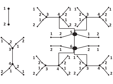
Figure 1: The single edge on the left hand size (top) is a good level $1$ tree. The tree on the left hand side (bottom) is a good level $2$ tree. The tree on the right hand size is a good level $3$ tree.

To complete the proof, we now show that there are enough good level $j$ trees, for $1\leq j\leq k$. For $k=1$, this is clearly true, since $a_{k}=2$ and one base edge suffices to force the algorithm to use $2$ colors. For $k\geq 2$, we note that, for $1\leq j<k$, good level $j$ trees are used to construct trees in all later batches. In each batch $i>j$, exactly $2a_{i}$ such trees are used. Thus, the total number of good level $j$ trees needed is

$$\sum_{i=j+1}^{k}2a_{i} =\sum_{i=j+1}^{k}4\cdot(8k^{3})^{k-i}=4\cdot\sum_{i=0}^{k-j-1}(8k^{3})^{i}=4\cdot\frac{(8k^{3})^{k-j}-1}{8k^{3}-1}<\frac{(8k^{3})^{k-j}}{k^{3}}$$

$$=\frac{a_{j}}{2k^{3}}$$

$$\leq\frac{a_{j}}{4k^{2}},\text{ since }k\geq 2$$

$$=g_{j},$$

where $g_{j}$ is the lower bound that we calculated on the number of good level $j$ trees.

If a connected graph is required, one vertex can be added to the last batch, connecting all trees remaining in the forest. ∎

It is easy to see that the construction in Lemma 1 can be changed to use many fewer vertices when considering bipartite graphs, rather than restricting to trees. For each bipartite graph in level $i$, it is sufficient to attach four good bipartite graphs from level $i-1$.

The following lemma holds for any graph, not only trees.

Lemma 2

There is a strictly $k$-competitive algorithm for $k$-batch coloring, even if $k$ is not known in advance.

Proof

Consider a graph $G$ presented in $k$ batches and let $\chi=\chi(G)$. Since each batch of vertices induces a subgraph of $G$, each batch can clearly be colored with at most $\chi$ colors. Thus, using the colors $(i-1)\chi+1,(i-1)\chi+2,\ldots,(i-1)\chi+\chi$ for batch $i$ yields a strictly $k$-competitive algorithm. ∎

Theorem 2.1 below follows directly from Lemmas 1 and 2.

Theorem 2.1

For any graph class containing trees as a special case, the optimal (strict) competitive ratio for $k$-batch coloring is $k$, regardless of whether or not $k$ is known in advance.

3 Interval Coloring in Two Batches

Since not all trees are interval graphs, the lower bound from the previous section does not apply here. For the case of interval graphs we show the surprising result that while coloring in two batches has a tight bound of $2$, the problem becomes easier if we assume that the vertices of the graph are revealed together with their interval representation (and this interval representation of vertices of the first batch cannot be modified in the second batch). The standard results for online coloring of interval graphs do not make this distinction: The lower bound is obtained for the (a priori easier) case where the interval representation of a vertex is revealed to the algorithm when the vertex is revealed, while the upper bound holds even if such a representation is not revealed (the online algorithm only computes a maximum clique size containing the new vertex and applies the First-Fit algorithm on a subset of the vertices). Throughout this section, our lower bounds are with respect to the asymptotic competitive ratio while our upper bounds are for the strict competitive ratio, and thus the results are tight for both measures.

3.1 Unknown interval representation

We start with a study of the case where the algorithm is guarantied that the resulting graph (at the end of every batch) will be an interval graph, but the interval representation of the vertices of the first batch is not revealed to the algorithm (and may depend on the actions of the algorithm). We show that in this case $2$ is the best competitive ratio that can be achieved by an online algorithm.

Theorem 3.1

For the problem of $2$-batch coloring of interval graphs with unknown interval representation, the optimal (strict) competitive ratio is $2$.

Proof

The upper bound follows from Lemma 2. Each of the two induced subgraphs is an interval graph, and it can be colored optimally in polynomial time even if the interval representation is not given.

Next, we show a matching lower bound. For a given $q\in\mathbb{N}$, let $N_{1}=\binom{4q}{q}+1$ and $N_{2}=\binom{4q}{2q}+1$. In the first batch, the adversary gives $N_{1}+N_{2}$ pairwise nonoverlapping cliques: $N_{1}$ cliques of size $q$ and $N_{2}$ cliques of size $2q$.

Assume that an algorithm uses at most $4q$ colors for the first batch. By the pigeon hole principle, there are two cliques of size $q$ that are colored with the same set $\mathcal{C}_{1}$ of colors. The vertices of these two cliques will correspond to the intervals $[5,6]$ and $[9,10]$, respectively. Similarly, there are two cliques of size $2q$ that are colored with the same set $\mathcal{C}_{2}$ of colors. For one of these cliques, $q$ vertices will correspond to the interval $[0,1]$ and the remaining $q$ vertices will correspond to the interval $[0,3]$. If any of these $2q$ vertices are colored with colors from $\mathcal{C}_{1}$, they will correspond to the interval $[0,1]$. We let $\mathcal{C}_{2}^{\prime}$ denote the set of colors used on the vertices corresponding to the interval $[0,3]$. Note that $\mathcal{C}_{1}\cap\mathcal{C}_{2}^{\prime}=\emptyset$, and hence, $|\mathcal{C}_{1}\cup\mathcal{C}_{2}^{\prime}|=2q$. For the other of these two cliques, the $q$ vertices colored with $\mathcal{C}_{2}^{\prime}$ will correspond to the interval $[12,15]$ and the remaining $q$ vertices will correspond to the interval $[14,15]$. All other intervals are placed to the right of the point $15$ so that they do not overlap with any of the four cliques just described.

The second batch consists of $q$ vertices corresponding to the interval $[2,8]$ and $q$ vertices corresponding to the interval $[7,13]$. All of these $2q$ intervals overlap with each other and with intervals of all colors in $\mathcal{C}_{1}\cup\mathcal{C}_{2}^{\prime}$. Thus, the algorithm uses at least $4q$ colors.

Since no clique is larger than $2q$ vertices, OPT uses $2q$ colors. Since $q$ can be arbitrarily large, this proves that no deterministic online algorithm can be better than $2$-competitive, even when considering the asymptotic competitive ratio. ∎

3.2 Known interval representation

We now assume that the vertices are revealed to the algorithm together with their interval representation. For this case, we show an improved competitive ratio of $\frac{3}{2}$. We first state the following lower bound whose proof is a special case of the lower bound proof of Kierstead and Trotter [14].

Lemma 3

For the problem of $2$-batch coloring of interval graphs with known interval representation, no algorithm can achieve a competitive ratio strictly smaller than $\frac{3}{2}$.

Proof

This is a special case of the lower bound of Kierstead and Trotter [14]. The construction is as follows. For a given $q\in\mathbb{N}$, let $N=\binom{3q}{2q}$. In the first batch, the adversary gives $2q$ vertices corresponding to the interval $[4i,4i+1]$, for $i=0,1,\ldots,N$. Thus, the first batch consists of $N+1$ pairwise nonoverlapping cliques. The clique of intervals $[4i,4i+1]$ is called clique $i$.

Assume that an algorithm colors the first batch using at most $3q$ colors. Since there are more than $N$ cliques, there must be two cliques, clique $k$ and clique $\ell$, colored with the same $2q$ colors. Assume that the cliques are named such that $k<\ell$.

In the second batch, the adversary gives $2q$ vertices corresponding to each of the intervals $[4k,4k+3]$ and $[4k+2,4\ell+1]$. To color the second batch vertices, the algorithm will need $4q$ colors different from the $2q$ colors used on clique $k$ and clique $\ell$. Thus, the algorithm uses at least $6q$ colors in total.

Since there is no clique larger than $4q$ vertices, OPT uses only $4q$ colors. Since $q$ can be chosen arbitrarily large, this shows that no deterministic online algorithm can be better than $\frac{3}{2}$-competitive. ∎

For the matching upper bound, we define an algorithm, TwoBatches, which is strictly $\frac{3}{2}$-competitive, using Algorithm 1 to color the first batch of intervals and Algorithm 2 to color the second batch. Intervals can be open, closed, or semi-closed.

Let $\omega$ denote the maximum clique size in the full graph consisting of intervals from both batches. For any interval $I$, let $\text{color}(I)$ denote the color assigned to $I$ by TwoBatches. Similarly, for a set $\mathcal{I}$ of intervals, $\text{color}(\mathcal{I})$ denotes the set of colors used to color the intervals in $\mathcal{I}$.

Each endpoint of a first batch interval $I$ is called an event point, and this event point is associated with $I$. If there is a point that is an endpoint of several intervals, we have multiple copies of this point as event points each of which is associated with a different interval.

We define a total order, $T$, on the event points. For two event points $p$ and $p^{\prime}$, if $p<p^{\prime}$, then $p$ appears before $p^{\prime}$ in the total order. For the case $p=p^{\prime}$, let $I$ and $I^{\prime}$ be the two intervals such that $p$ and $p^{\prime}$ are associated with $I$ and $I^{\prime}$, respectively. We consider a total order satisfying the following properties.

1. If $p$ and $p^{\prime}$ are both right endpoints, $p\notin I$, and $p^{\prime}\in I^{\prime}$, then $p$ appears before $p^{\prime}$ in the total order of the event points.

2. Otherwise, if $p$ is a left endpoint and $p^{\prime}$ is an right endpoint, then:

   • If $p\notin I$, then $p^{\prime}$ appears before $p$ in the total order of the event points.

   • If $p\in I$ and $p^{\prime}\notin I^{\prime}$, then $p^{\prime}$ appears before $p$ in the total order of the event points.

   • If $p\in I$ and $p^{\prime}\in I^{\prime}$, then $p$ appears before $p^{\prime}$ in the total order of the event points.

3. Otherwise (that is, $p$ and $p^{\prime}$ are both left endpoints), then if $p\in I$ and $p^{\prime}\notin I^{\prime}$, then $p$ appears before $p^{\prime}$ in the total order of the event points.

We fix one particular total order, $T$, on the event points satisfying all these conditions. Observe that this total order is a refinement of the standard order “$\leq$” on the real numbers. If an event point $p$ appears before another event point $q$ in $T$, we write $p<_{T}q$. If $p$, $q$, and $p^{\prime}$ are event points, we say that $q$ is between $p$ and $p^{\prime}$, if and only if $p<_{T}q<_{T}p^{\prime}$. In this case, we will also sometimes say that $q$ is to the right of $p$ and to the left of $p^{\prime}$.

For any three points $p$, $q$, and $p^{\prime}$, where $q$ is not an event point, we say that $q$ is between $p$ and $p^{\prime}$, if and only if $p<q<p^{\prime}$. In this case, we will also sometimes say that $q$ is to the right of $p$ and to the left of $p^{\prime}$.

3.2.1 First batch.

Algorithm 1 processes the event points in the order given by $T$. When a right endpoint is processed, we say that the color of the associated interval is released. It is then available until it is used again. When processing a left endpoint, the associated interval is colored with the most recently released available color (or a new color, if necessary). Thus, a stack ordering is used for the colors. Pseudo-code for the algorithm is given in Algorithm 1.

1:  $\omega_{1}\leftarrow$ maximum clique size in the first batch

2:  Initialize an empty stack of colors // The stack will contain available colors

3:  for $i\leftarrow\omega_{1}$ downto $1$ do

4:        $\text{Push}(i)$

5:  for each event point, $p$, in the order given by $T$ do

6:        if $p$ is a left endpoint of an interval $I$ then

7:              $\text{color}(I)\leftarrow\text{Pop}(){}$

8:        else if $p$ is a right endpoint of an interval $I$ then

9:              $\text{Push}(\text{color}(I))$

Algorithm 1 Coloring the first-batch intervals.

For ease of presentation, we insert $2\omega$ dummy intervals into the first batch: one clique of size $\omega$ before all input intervals and one clique of size $\omega$ after all input intervals. Since these dummy cliques do not overlap with any other intervals, each will be colored with the colors $1,2,\ldots,\omega$, and they will not influence the behavior of Algorithm 1 on the rest of the first-batch intervals.

We note that it is well-known that one can color an interval graph with a maximum clique size of $\omega$ using $\omega$ colors, by maintaining a set of available colors, and traversing the event points according to the total order $T$: Each time a left endpoint is considered, we color its associated interval with one of the colors in the set of available colors (removing it from this set), and each time a right endpoint is considered we return the color of its interval to the set of available colors. By using Algorithm 1, we consider one particular tie-breaking rule used whenever the set of available colors contains more than one color. More commonly, one considers the First-Fit rule of using the minimum color in the set of available colors. However, in order to establish the improved bound of $\frac{3}{2}$ on the strict competitive ratio (or even for the competitive ratio) of the algorithm for two batches, we need to use a different tie-breaking rule, the one defined by using a stack as in Algorithm 1.

Before analyzing the algorithm, we introduce some additional terminology. Maximal cliques always refer only to first-batch intervals. For each maximal clique, we choose a point, called a clique point, contained in all intervals of the clique. If a clique point $p$ appears to the right of another clique point $q$, we say that the clique corresponding to $p$ appears to the right of the clique corresponding to $q$, and vice versa.

For each maximal clique, $\mathcal{I}$, we order the intervals of the clique by left and right endpoints, respectively, resulting in two orderings, $L_{\mathcal{I}}(\cdot)$ and $R_{\mathcal{I}}(\cdot)$. The further an endpoint is from the clique point of $\mathcal{I}$, the earlier the interval appears in the ordering. More precisely, for each interval $I\in\mathcal{I}$, $L_{\mathcal{I}}(I)=i$, if the left endpoint of $I$ appears as the $i$th in $T$ among the endpoints associated with intervals in $\mathcal{I}$. Similarly, $R_{\mathcal{I}}(I)=j$, if the right endpoint of $I$ appears as the $j$th last in $T$ among the endpoints associated with intervals in $\mathcal{I}$. As an example, consider the clique $\mathcal{I}$ consisting of the three intervals $a=[1,6]$, $b=[2,4]$, and $c=[3,5]$. For this clique, we have $L_{\mathcal{I}}(a)=1$, $L_{\mathcal{I}}(b)=2$, $L_{\mathcal{I}}(c)=3$ and $R_{\mathcal{I}}(a)=1$, $R_{\mathcal{I}}(b)=3$, $R_{\mathcal{I}}(c)=2$.

The following lemma is illustrated in Figure 2.

Figure 2: Illustration of Lemma 4, with $h=3$. The intervals of $\mathcal{I}^{\prime}$ are drawn with dashed lines.

Lemma 4

Consider a maximal clique, $\mathcal{I}_{\ell}$, of size $m$ and an interval $I_{\ell}\in\mathcal{I}_{\ell}$ such that $R_{\mathcal{I}_{\ell}}(I_{\ell})=0pt$. Let $\mathcal{I}_{\ell}^{0pt}=\left\{I\in\mathcal{I}_{\ell}\mid R_{\mathcal{I}_{\ell}}(I)<0pt\right\}$ be the $0pt-1$ intervals in $\mathcal{I}_{\ell}$ with the rightmost right endpoints. Let $\mathcal{I}_{r}$ be the first maximal clique of size at least $0pt$ to the right of $\mathcal{I}_{\ell}$ and let $I_{r}\in\mathcal{I}_{r}$ be such that $L_{\mathcal{I}_{r}}(I_{r})=0pt$. Finally, let $p_{\ell}$ be the right endpoint of $I_{\ell}$, let $p_{r}$ be the left endpoint of $I_{r}$, and consider the set $\mathcal{I}^{\prime}$ of first-batch intervals containing a point $p$ with $p_{\ell}<p<p_{r}$ or an endpoint $p$ with $p_{\ell}<_{T}p<_{T}p_{r}$. Then, $\text{color}(\mathcal{I}^{\prime})\subseteq\text{color}(\mathcal{I}_{\ell}^{0pt})\,.$

Proof

For the intervals in $\mathcal{I}_{\ell}^{0pt}$, the lemma follows trivially.

We now consider the intervals in $\mathcal{I}^{\prime}\setminus\mathcal{I}_{\ell}^{0pt}$. Note that we can assume $p_{\ell}<_{T}p_{r}$, since otherwise $\mathcal{I}^{\prime}$ is empty, and the lemma follows trivially.

Assume for the sake of contradiction that some interval $I^{\prime}\in\mathcal{I}^{\prime}\setminus\mathcal{I}_{\ell}^{0pt}$ has an endpoint to the left of $p_{\ell}$. This interval would overlap with all intervals in $\mathcal{I}_{\ell}^{0pt}$, contradicting the assumption that $p_{\ell}<_{T}p_{r}$. Hence, we only need to consider intervals with a left endpoint between $p_{\ell}$ and $p_{r}$.

Consider any interval with a left endpoint $p$ such that $p_{\ell}<_{T}p<_{T}p_{r}$. It follows from the definition of $\mathcal{I}_{r}$ and $I_{r}$ that there are more right endpoints than left endpoints between $p_{\ell}$ and $p$ (note that $0pt>1$ in this case). Thus, at $p$, the most recently released available color is a color in $\text{color}(\mathcal{I}_{\ell}^{0pt})$, and therefore, the interval associated with $p$ is colored with a color in $\text{color}(\mathcal{I}_{\ell}^{0pt})$. ∎

3.2.2 Second batch.

We now describe the algorithm, Algorithm 2, given in pseudo-code below, for coloring the second batch intervals.

A chain is a set of nonoverlapping second batch intervals. The algorithm starts with partitioning the second-batch intervals into $\omega$ chains (some of which may be empty). This is clearly possible, since the graph is $\omega$-colorable.

The second batch intervals are colored in iterations, two chains per iteration. The algorithm keeps a counter, $i$, which is incremented once in each iteration, and maintains the set $\textsc{Batch}_{2}\textsc{-Colored}$ of second batch intervals that the algorithm has already colored. In each iteration, a set of nonoverlapping first-batch intervals is processed. The algorithm maintains the invariant that, at the beginning of each iteration, any maximal first-batch clique of size $0pt$ contains exactly $\min\{0pt,\omega-i\}$ unprocessed intervals.

A first-batch maximal clique of size at least $\omega-i+1$ as well as its clique point is said to be active. The part of the real line between two neighboring active clique points is called a region. Throughout the execution of Algorithm 2, the number of regions is nondecreasing, and whenever a region is split, the chains of the region are also split by a simple projection onto each region and each resulting region will contain its boundary active clique points (in particular, this means that active clique points may belong to two regions). In each iteration, each region and its chains are treated separately.

The algorithm maintains the invariant that no uncolored second batch interval overlaps with more than one region. This is the key property, allowing the algorithm to consider one region at a time in a given iteration of the algorithm. First-batch intervals overlapping with more than one region will be cut into more intervals, with a cutting point at each active clique point contained in the interval. Thus, by cutting the intervals of an active clique of size $0pt$, the clique is replaced by two cliques of size $0pt$ in neighboring regions. When a first-batch interval is cut into parts, the different parts of the interval may be processed in different iterations, but no new event points are introduced.

In the $i$th iteration, one chain in each region is colored with the color of a first-batch interval in the region being processed in this iteration, and another chain of the region will be colored with the color $\omega+i$, which has not been used in the region before. For any point $p$, let $d_{p}$ be the number of second batch intervals containing $p$. We say that $p$ is covered by a set $S$ of intervals, if there are $\min\{d_{p},i\}$ second batch intervals in $S$ containing $p$.

Next, we define a set ${\mathcal{P}}$ of representative points, such that each interval between two neighboring clique points is represented by one point. To this end, we define the following equivalence relation between points on the real line. For a pair of points $p$ and $p^{\prime}$, we say that $p$ is equivalent to $p^{\prime}$ if the following conditions hold:

• For every clique point $q$, either both $p\leq q$ and $p^{\prime}\leq q$ or both $p\geq q$ and $p^{\prime}\geq q$ (this in particular means that $p$ and $p^{\prime}$ belong to a common region).

• For every interval $I$ of either the first batch or the second batch, we have that either $p,p^{\prime}\in I$ or the two points $p$ and $p^{\prime}$ are to a common side of $I$ (either both are smaller than any point in $I$ or both are larger than any point in $I$).

Observe that the number of equivalence classes of this relation is linear in the number of intervals of the input. The set of representative points ${\mathcal{P}}$ is defined such that each equivalence class has exactly one member in ${\mathcal{P}}$, chosen arbitrarily. We use the following observation.

Observation 3.2

For a given set $S$ of intervals, at any point after line 9 in Algorithm 2, we have that all points (on the real line) are covered by $S$ if and only if all points in ${\mathcal{P}}$ are covered by $S$.

For a region $R$, we denote by ${\mathcal{P}}_{R}$ the set of representative points contained in region $R$ (that is, ${\mathcal{P}}_{R}=R\cap{\mathcal{P}}$).

1:  Mark all first-batch intervals as unprocessed

2:  Create an optimal coloring of the second-batch intervals, using a set $\mathcal{C}$ of $\omega$ colors

3:  $R\leftarrow(-\infty,\infty)$ // Initially, there is only one region

4:  $\textsc{Chains}_{R}\leftarrow\emptyset$

5:  ${\mathcal{P}}_{R}\leftarrow$ the set of representative points in region $R$

6:  for each color $c\in\mathcal{C}$ do

7:     $\textsc{Chains}_{R}\leftarrow\textsc{Chains}_{R}\cup\{\{I\mid I\text{ is a second batch interval with color }c\}\}$

8:  $\textsc{Batch}_{2}\textsc{-Colored}\leftarrow\emptyset$ // Set of colored second batch intervals

9:  $i\leftarrow 0$

10:  while $i<\lfloor\omega/2\rfloor$ do // Invariant $I$

11:     // Color two chains:

12:     $i\leftarrow i+1$

13:     Split all regions (incl. the assoc. chains and sets of repr. points) at all active clique points

14:     for each region $R$ containing at least one nonempty chain do

15:       $(\textsc{Chain}_{1},\textsc{Chain}_{2})\leftarrow$ CreateChains($R$) // See Algorithm 3

16:       // Color intervals in $\textsc{Chain}_{1}$ and $\textsc{Chain}_{2}$ using a first batch color and a new color:

17:       $I_{\ell}\leftarrow$ the unprocessed first-batch interval of the earliest event point in $R$

18:       $I_{r}\leftarrow$ the unprocessed first-batch interval of the latest event point in $R$

19:       Mark $I_{\ell}$ and $I_{r}$ as processed

20:       Give all intervals in $\textsc{Chain}_{1}$ the color of $I_{\ell}$

21:       Give all intervals in $\textsc{Chain}_{2}$ the color $\omega+i$

22:       $\textsc{Batch}_{2}\textsc{-Colored}\leftarrow\textsc{Batch}_{2}\textsc{-Colored}\cup\textsc{Chain}_{1}\cup\textsc{Chain}_{2}$

23:       $\textsc{Chain}_{R}\leftarrow\textsc{Chain}_{R}\setminus\{\textsc{Chain}_{1},\textsc{Chain}_{2}\}$

24:  // If $\omega$ is odd, each region may have one chain left to color:

25:  for each region $R$ where $\textsc{Chains}_{R}$ contains a nonempty chain Chain do

26:     $I\leftarrow$ the unprocessed first-batch interval with the earliest event point in $R$

27:     Give the intervals of Chain the color of $I$

Algorithm 2 Coloring the second batch intervals.

1:  $\textsc{Chain}_{1}$ $\leftarrow$ a chain in $\textsc{Chains}_{R}$ containing the leftmost left endpoint

2:  $\textsc{Chain}_{2}$ $\leftarrow$ any other chain from $\textsc{Chains}_{R}$

3:  while some point in ${\mathcal{P}}_{R}$ is not covered by $\textsc{Batch}_{2}\textsc{-Colored}\cup\textsc{Chain}_{1}\cup\textsc{Chain}_{2}$  do

4:     $p\leftarrow$ the leftmost point in ${\mathcal{P}}_{R}$ not covered by $\textsc{Batch}_{2}\textsc{-Colored}\cup\textsc{Chain}_{1}\cup\textsc{Chain}_{2}$

5:     $\textsc{Chain}_{3}$ $\leftarrow$ a chain from $\textsc{Chains}_{R}$ containing $p$

6:     if for all points $q<p$ in ${\mathcal{P}}_{R}$, $q$ is contained in $\textsc{Chain}_{3}$ or in both $\textsc{Chain}_{1}$ and $\textsc{Chain}_{2}$ then

7:       $\textsc{Chain}_{2}$ $\leftarrow$ $\textsc{Chain}_{3}$ // $\textsc{Chain}_{2}$ now refers to the chain in $\textsc{Chains}_{R}$ that $\textsc{Chain}_{3}$ refers to

8:     else

9:       $q\leftarrow$ the rightmost point in ${\mathcal{P}}_{R}$ left of $p$ violating the condition

10:       $\textsc{Chain}\leftarrow$ one of $\textsc{Chain}_{1}$ or $\textsc{Chain}_{2}$ not containing $q$ // Chain now refers to a chain in $\textsc{Chains}_{R}$

11:       // Do a crossover of Chain and $\textsc{Chain}_{3}$ at the point $q$, modifying Chain and $\textsc{Chain}_{3}$ in $\textsc{Chains}_{R}$:

12:       $\textsc{Tail}\leftarrow\{I\in\textsc{Chain}\mid I\text{ starts to the right of }q\}$

13:       $\textsc{Tail}_{3}\leftarrow\{I\in\textsc{Chain}_{3}\mid I\text{ starts to the right of }q\}$

14:       $\textsc{Chain}\leftarrow(\textsc{Chain}\setminus\textsc{Tail})\cup\textsc{Tail}_{3}$

15:       $\textsc{Chain}_{3}\leftarrow(\textsc{Chain}_{3}\setminus\textsc{Tail}_{3})\cup\textsc{Tail}$

16:  return  $(\textsc{Chain}_{1},\textsc{Chain}_{2})$

Algorithm 3 CreateChains($R$)

We use the following loop invariant for each region to establish that TwoBatches is correct and strictly $3/2$-competitive. The proof of the invariant $I$ is based on induction on the value of $i$.

Invariant $\boldsymbol{I}$:

1. All points $p$ are covered by the set $\textsc{Batch}_{2}\textsc{-Colored}$.

2. No color used for an unprocessed first-batch interval contained in a region $R$ has been used for a second batch interval intersecting region $R$ so far.

3. Each active clique has exactly $\omega-i$ unprocessed intervals.

4. For each region $R$, $\textsc{Chain}_{R}$ has at most $\omega-2i$ chains.

Lemma 5

$I$ is an invariant for the while-loop in Algorithm 2.

Proof

We prove by on induction on $i$ that the invariant holds at the start of every iteration of the while-loop.

1. By Observation 3.2, it suffices to show that the set $\textsc{Batch}_{2}\textsc{-Colored}$ covers all points in ${\mathcal{P}}$.

   At the beginning of the first iteration, $i=0$, so (I1) is trivially true. At the beginning of each of the following iterations, it follows from (I1) that each point $p$ is contained in at least $\min\{d_{p},i\}$ intervals in $\textsc{Batch}_{2}\textsc{-Colored}$. In line 22, all intervals of $\textsc{Chain}_{1}\cup\textsc{Chain}_{2}$ are added to $\textsc{Batch}_{2}\textsc{-Colored}$. Thus, we only need to prove that, if $p$ is not covered after the increment of $i$ in line 12, the while loop in lines 3–15 of Algorithm 3 will add at least one interval containing $p$ to $\textsc{Chain}_{1}\cup\textsc{Chain}_{2}$.

   Consider a region $R$ and let $p_{\ell}$ and $p_{r}$ be defined as in Lemma 4, with $0pt=\omega-i+1$. Any point in $R$ to the left of $p_{\ell}$ or to the right of $p_{r}$ is contained in at least $0pt$ first-batch intervals. Hence, there cannot be any uncovered points in $R$ to the left of $p_{\ell}$ or to the right of $p_{r}$.

   As long as some point $p$ in ${\mathcal{P}}_{R}$ is not covered by $\textsc{Batch}_{2}\textsc{-Colored}\cup\textsc{Chain}_{1}\cup\textsc{Chain}_{2}$, it follows from (I1) and the definition of covered that $\textsc{Chains}_{R}$ contains $p$ and that $\textsc{Chain}_{1}\cup\textsc{Chain}_{2}$ does not contain $p$. Thus, $\textsc{Chain}_{3}$ of line 5 of Algorithm 3 exists.

   If for all points $q<p$ in ${\mathcal{P}}_{R}$, $\textsc{Chain}_{3}$ contains $q$ or both $\textsc{Chain}_{1}$ and $\textsc{Chain}_{2}$ contain $q$, swapping any of $\textsc{Chain}_{1}$ or $\textsc{Chain}_{2}$ with $\textsc{Chain}_{3}$ will ensure that $\textsc{Chain}_{1}\cup\textsc{Chain}_{2}$ contains all points $q\leq p$ in ${\mathcal{P}}_{R}$.

   Otherwise, there is a point $q<p$ in ${\mathcal{P}}_{R}$ not contained in $\textsc{Chain}_{3}$ and not contained in both $\textsc{Chain}_{1}$ and $\textsc{Chain}_{2}$. The algorithm chooses $q$ as the rightmost such point among the points in ${\mathcal{P}}_{R}$. The algorithm then chooses a $\textsc{Chain}\in\{\textsc{Chain}_{1},\textsc{Chain}_{2}\}$ such that Chain does not contain $q$. Since neither Chain nor $\textsc{Chain}_{3}$ contains $q$, all intervals in $\textsc{Chain}\cup\textsc{Chain}_{3}$ appear strictly before or after $q$. Thus it is possible to cut each of Chain and $\textsc{Chain}_{3}$ into two sets, “head” and “tail” consisting of the intervals ending before $q$ or starting after $q$, respectively, and let the two chains swap tails, while maintaining the property that no two intervals within a chain overlap.

   After this crossover operation, $p$ is contained in Chain. Neither $\textsc{Chain}_{1}$ nor $\textsc{Chain}_{2}$ is changed to the left of $q$. Since all points between $q$ and $p$ were contained in $\textsc{Chain}_{3}$ or both $\textsc{Chain}_{1}$ and $\textsc{Chain}_{2}$ before the crossover, all such points are still contained in $\textsc{Chain}_{1}\cup\textsc{Chain}_{2}$ after the crossover. Thus, the leftmost point in ${\mathcal{P}}_{R}$ not covered by $\textsc{Batch}_{2}\textsc{-Colored}\cup\textsc{Chain}_{1}\cup\textsc{Chain}_{2}$ now occurs at or to the right of the leftmost point in ${\mathcal{P}}_{R}$ to the right of $p$. This means that, after $O(n)$ iterations of the while loop of lines 3–15 of Algorithm 3, all points in ${\mathcal{P}}$ are covered by $\textsc{Batch}_{2}\textsc{-Colored}\cup\textsc{Chain}_{1}\cup\textsc{Chain}_{2}$.

2. At the beginning, the statement is trivially true, since no second-batch interval has been colored.

   Since no unprocessed first-batch intervals in a region are colored with $\text{color}(I_{\ell})$, according to Lemma 4, and since no first-batch intervals are colored with $\omega+i$, (I2) is maintained.

3. At the beginning of the first iteration, (I3) is trivially true, since every active clique has $\omega$ first-batch intervals, and all first-batch intervals are unprocessed.

   In each iteration, the cliques of size $\omega-i+1$ are added to the set of active cliques, and one interval of each active clique is processed. Hence, (I3) is maintained.

4. At the beginning, the statement holds as an optimal coloring consists of exactly $\omega$ color classes and the number of chains in $\textsc{Chain}_{R}$ after line 7 is the number of color classes.

   In each iteration of the while loop in lines 3–15 of Algorithm 3, the number of chains in $\textsc{Chain}_{R}$ is not modified, as in each such iteration we replace two chains by another pair of chains covering the same set of second batch intervals. Invariant (I4) is maintained because the number of chains in $\textsc{Chain}_{R}$ is modified once in every iteration in line 22, where it is decreased by two.

∎

We use the invariant $I$ to prove that for any input $\sigma$, TwoBatches produces a proper coloring using at most $\left\lfloor\frac{3}{2}\textsc{OPT}(\sigma)\right\rfloor$ colors.

Lemma 6

For any input $\sigma$, the algorithm TwoBatches produces a proper coloring using at most $\left\lfloor\frac{3}{2}\textsc{OPT}(\sigma)\right\rfloor$ colors.

Proof

We first note that, by (I1), no chain in $\textsc{Chains}_{R}$ can contain an active clique point. Thus, the splitting of chains done in line 13 is possible.

In each of the $\lfloor\omega/2\rfloor$ iterations of the while loop of lines 3–15 of Algorithm 3, two chains are colored and the number of chains in $\textsc{Chain}_{R}$ is decreased by two. If $\omega$ is odd, one additional chain may be colored in line 27 (and at this point $\textsc{Chain}_{R}$ consists of a single chain by invariant (I4)). Thus, all of the $\omega$ chains containing all second batch intervals are colored.

The actual coloring happens in lines 20 and 21, and possibly in line 27. In line 20, the color used is the color, $c$, of the earliest event point associated with the unprocessed first-batch interval, $I_{\ell}$, in the region $R$. By Lemma 4 and (I3), $I_{\ell}$ and $I_{r}$ are the only first-batch intervals overlapping with $R$ that are colored with $c$. By invariant (I1) and the definition of $I_{\ell}$ and $I_{r}$, no interval in $\textsc{Chains}_{R}$ overlaps with $I_{\ell}$ and $I_{r}$ in $R$. By invariant (I2), no second batch interval in $R$ has been colored with $c$ in earlier iterations. Thus, coloring the intervals of $\textsc{Chain}_{1}$ results in a legal coloring of these intervals. The same arguments hold for the possible coloring done in line 27. Since the color $\omega+i$ has never been used before, the coloring of $\textsc{Chain}_{2}$ is also legal.

In summary, in Algorithm 1, $\omega$ colors are used. In Algorithm 2, the colors are used again for some intervals and only $\left\lfloor\omega/2\right\rfloor$ new colors are used. ∎

Combining Lemmas 3 and 6 shows that the optimal (strict) competitive ratio for the problem is $\frac{3}{2}$:

Theorem 3.3

TwoBatches has a strict competitive ratio of $\frac{3}{2}$.

4 Sum Coloring of Graphs in Multiple Batches

We study two cases separately: the case where the number of batches is known to the algorithm from the beginning, and the case where it is not. Once again, our lower bounds are for the competitive ratio and our upper bounds are for the strict competitive ratio.

4.1 Number of batches known in advance

We start our study of sum coloring by examining the case where the algorithm knows the number of batches $k$ in advance. Recall that we do not require that algorithms used within one batch be polynomial time.

Lemma 7

There is a strictly $k$-competitive algorithm for sum coloring in $k$ batches, if $k$ is known in advance.

Proof

For each batch, the algorithm, $k$-BatchColor, applies an optimal procedure, Color, to compute an optimal sum coloring for the subgraph induced by the set of vertices of batch $i$, separately from previous batches. In order to construct the solution of the input graph, $k$-BatchColor applies the following transformation: For every vertex $v$ of batch $i$, if Color colors $v$ with color $c$, then $k$-BatchColor colors $v$ using color $f(i,c)=k\cdot(c-1)+i$. This function $f$ satisfies $f(i,c)\equiv i\ (\bmod\ k)$, so if $f(i,c)=f(i^{\prime},c^{\prime})$, for some $1\leq i,i^{\prime}\leq k$, then $i=i^{\prime}$. Moreover, if $f(i,c)=f(i,c^{\prime})$, then $k(c-c^{\prime})=0$, and therefore $c=c^{\prime}$. Thus, vertices of different batches have different colors, and two vertices of the same batch have the same color after the transformation if and only if they had the same color in the solution returned by Color. As any proper coloring of the graph provides proper colorings for the $k$ induced subgraphs, the total cost of the $k$ outputs of Color does not exceed the cost of an optimal coloring of the entire graph. For any color $c$ and batch $i$, $f(i,c)\leq k\cdot c$. Thus, the cost of the output is at most $k$ times the total cost of the $k$ solutions returned by Color (for the $k$ vertex disjoint induced subgraphs). ∎

We prove a matching lower bound for this case, which holds even for the asymptotic competitive ratio.

Lemma 8

No algorithm for sum coloring in $k$ batches has a competitive ratio strictly smaller than $k$, even if $k$ is known in advance.

Proof

Assume for the sake of contradiction that there is a value of $k$ and an online algorithm $A$ for sum coloring of graphs in $k$ batches whose competitive ratio $\rho$ is strictly smaller than $k$. Let $M$ be a large integer such that $M>\max\{2k^{2},\frac{2\rho}{k-\rho}\}$.

The algorithm will be presented with $k$ batches, such that after every batch $i$ ($1\leq i\leq k$) the input either stops (the remaining $k-i$ batches will be empty), or one vertex of the batch, which will be denoted by $v_{i}$, is selected as a designated vertex, and it will be used for constructing the other batches.

Batch $i$ (for $i=1,2,\ldots,k$) is constructed as follows: The batch consists of a set $V_{i}$ of $M^{i}$ vertices, each of which has $i-1$ neighbors that are $v_{1},v_{2},\ldots,v_{i-1}$ (thus, the vertices of $V_{i}$ form an independent set and the vertices $v_{1},v_{2},\ldots,v_{i}$ form a clique). For $i\leq k-1$, if the algorithm colors all vertices of batch $i$ with colors of value at least $k$, then the input stops. Otherwise, one vertex whose color is in $\{1,2,\ldots,k-1\}$ is selected to be $v_{i}$, and the set of vertices of the next batch, $V_{i+1}$, is presented. If the input consists of $j$ batches, $V=\cup_{i=1}^{j}V_{i}$.

We compute an upper bound on the optimal sum of colors, if the input stops after the first $j$ batches (we describe solutions which are not necessarily optimal). If the input consists of $j$ batches, we next show that the set $V\setminus\{v_{1},v_{2},\ldots,v_{j-1}\}$ is independent. Consider a vertex $v$ of batch $i$. This vertex is presented with edges to $\{v_{1},v_{2},\ldots,v_{i-1}\}$. If $v$ does not become $v_{i}$, it will not have any further edges. Thus, it is possible to assign color $1$ to each such vertex, and use color $i+1$ for $v_{i}$. We show that, for $1\leq j\leq k$, this gives a total cost of $O_{j}\leq M^{j}+2M^{j-1}$. For $j=1$ and $j=2$, we obtain $O_{1}=M$ and $O_{2}=M^{2}+M+1\leq M^{2}+2M$. For $j\geq 3$, the total cost of this solution is

$$O_{j} =\sum_{i=1}^{j}(M^{i}-1)+1+\sum_{i=1}^{j-1}(i+1)=\sum_{i=1}^{j}M^{i}+\sum_{i=1}^{j-1}i=\frac{M^{j+1}-1}{M-1}-1+\frac{j(j-1)}{2}$$

$$<\frac{M^{j+1}}{M-1}+k^{2}<\frac{M^{j+1}}{M-1}+M^{j-2},\text{ as $j-2\geq 1$.}$$

We find that

$$\frac{M^{j+1}}{M-1}+M^{j-2} \leq M^{j}+2M^{j-1}$$

$$\Leftrightarrow \frac{M^{3}}{M-1}+1 \leq M^{2}+2M$$

$$\Leftrightarrow \;M^{3}+M-1 \leq M^{3}+2M^{2}-M^{2}-2M$$

$$\Leftrightarrow 3M \leq M^{2}+1,\text{ which holds for any }M\geq 3.$$

If the input stops after $j<k$ batches, then $A$ has colored $M^{j}$ vertices with colors of at least $k$, and its cost is at least $k\cdot M^{j}$. Otherwise, consider batch $k$. Each of the vertices $v_{1},v_{2},\ldots,v_{k-1}$ was given a color no larger than $k-1$, and since they induce a clique, each of the colors $\{1,2,\ldots,k-1\}$ is used exactly once on these $k-1$ vertices. When the set $V_{k}$ is presented, each vertex of $V_{k}$ is connected to each vertex in $\{v_{1},v_{2},\ldots,v_{k-1}\}$, so every vertex of $V_{k}$ must be colored with a color that is at least $k$. Thus, in this batch the total cost of the algorithm is at least $k\cdot M^{k}$.

We showed that if the input stops after batch $j$ (for $1\leq j\leq k$), the cost of the algorithm is at least $k\cdot M^{j}$, while the cost of an optimal solution does not exceed $M^{j}+2M^{j-1}$. The performance ratio is thus at least

$$\frac{k\cdot M^{j}}{M^{j}+2M^{j-1}}=\frac{k}{1+2/M}>\frac{k}{1+2(k-\rho)/(2\rho)}=\frac{2\rho k}{2\rho+2k-2\rho}=\rho\,,$$

as $M>\frac{2\rho}{k-\rho}$. This contradicts the assumption that the competitive ratio was $\rho$. ∎

Combining Lemmas 7 and 8 gives the following result:

Theorem 4.1

For sum coloring in $k$ batches, with $k$ known in advance, the optimal (strict) competitive ratio is $k$.

Remark 1

Observe that the graph in the proof of Lemma 8 for the case $k=2$ has no cycles. Thus, there is no online algorithm for sum coloring of forests in $k$ batches with competitive ratio strictly smaller than $2$. This can be strengthened to trees by adding one extra vertex in the second batch which is adjacent to all of the isolated vertices from the first batch.

Theorem 4.2

For sum coloring of trees in $k$ batches, First-Fit is strictly $2$-competitive, and this is the best possible competitive ratio, even if $k$ is known in advance.

Proof

The lower bound of $2$ for any online algorithm holds because the graph in the proof of Lemma 8 for the case $k=2$ has no cycles, and thus there is no online algorithm for sum coloring of forests in $2$ batches whose competitive ratio is strictly smaller than 2. This can be extended to trees by adding one extra vertex in the second batch which is adjacent to all vertices of the first batch. To prove the upper bound of First-Fit, we will show by induction on $t$ that when First-Fit is used for coloring a tree (a connected subgraph) on $t$ vertices the sum of the colors of the vertices is at most $2t-1$. Obviously, no algorithm can have a cost below $t$ (in fact, if $t>1$, then any coloring has cost at least $t+1$).

For $t=1$, the claim follows trivially as a single vertex is assigned color $1$. Assume that the claim holds for all $t^{\prime}<t$ and we prove it for $t$. Consider the last vertex to be colored by First-Fit. This vertex will be connected to some number of existing trees (connected components of the graph prior to this iteration), and we denote this number (of components) by $X$. If $X=0$, then the new vertex gets color $1$ and becomes a singleton (so $t=1$ and the sum of colors is $1=2t-1$). If $X>0$, then for every $j=1,2,\ldots,X$, the $j$-th tree with $t_{j}$ vertices had the sum of colors $2t_{j}-1$ (or less). The new vertex has a color not exceeding $X+1$ (as the new vertex is connected to one vertex of each of the $X$ existing trees), and we have $\sum_{j=1}^{X}t_{j}=t-1$. We find that the total cost of the solution returned by First-Fit does not exceed $\sum_{j=1}^{X}(2t_{j}-1)+X+1=2(t-1)-X+(X+1)=2t-1$. ∎

4.2 Number of batches unknown in advance

Next, we consider the case where the number of batches $k$ is not known in advance. Thus, to obtain a given competitive ratio, this ratio must be obtained after each batch. Note that the algorithm described in the proof of Lemma 7 cannot be used in this case. While the algorithm is not well defined if $k$ is unknown in advance to the algorithm, it may seem that modifying the value of $k$ by doubling would result in a competitive ratio of $O(k)$, but no such algorithm exists. We prove that for any positive nondecreasing sequence $f(i)$, which is defined for integer values of $i$ (where $f(i)\geq 1$ for $i\geq 1$), no algorithm with competitive ratio $O(f(k))$ can be given if the series $S_{f}=\sum_{i=1}^{\infty}\frac{1}{f(i)}$ is divergent. On the other hand, we show that if this series is convergent, then such an algorithm can be given. This shows, in particular, that the best possible competitive ratio is $O(k\log k(\log\log k)^{2})$ (since the series for this function converges according to the Cauchy condensation test), and it is $\Omega(k\log k\log\log k)$ (since the series for this function diverges according to the Cauchy condensation test). In fact it is $O(k\log k\log\log k\cdots$ $(\log^{(x)}k)^{2})$ and $\Omega(k\log k\log\log k\cdots\log^{(x)}k)$, for any positive integer $x$.

Consider a sequence $f(i)$ for which $S_{f}$ is convergent, and let $c_{f}$ be its limit. We present an algorithm, $\textsc{BatchColor}_{f}$, for this variant of sum coloring. Initially, all colors are declared available. When coloring the $i$th batch, its induced subgraph is first colored using an optimal procedure, Color. Let $t_{i}$ denote the maximum color used by Color for batch $i$. For each $j=1,2,\ldots,t_{i}$ in increasing order, vertices that Color gives color $j$ will be colored using the largest available color among the colors $1,2,\ldots,\lfloor j\cdot c_{f}\cdot f(i)\rfloor$. Then, this color is declared taken. This color is now unavailable for vertices of future batches and for vertices of the current batch that were assigned a color larger than $j$ by Color. If this process is successful (there always exists an available color), then we say that batch $i$ is feasible.

Assuming that all batches are feasible, using arguments similar to those used for Lemma 7, we obtain an upper bound on the competitive ratio of $\textsc{BatchColor}_{f}$ as follows. Since a color used by Color in a particular batch is assigned to an available color by $\textsc{BatchColor}_{f}$, if all batches are feasible, each pair, $(i,j)$, where $i$ is a batch number and $j$ is a color assigned by Color in batch $i$, is given a different color. Since Color produces a proper coloring, $\textsc{BatchColor}_{f}$ does too. The function $f$ is nondecreasing, so the color assigned to a given vertex by $\textsc{BatchColor}_{f}$ is at most $c_{f}\cdot f(k)$ times the color assigned by Color.

Lemma 9

Consider sum coloring in $k$ batches, where the value of $k$ is not known in advance. If for all $1\leq i\leq k$, batch $i$ is feasible, then the competitive ratio of $\textsc{BatchColor}_{f}$ is at most $c_{f}\cdot f(k)$.

Lemma 10

All batches for the algorithm $\textsc{BatchColor}_{f}$ are feasible.

Proof

Assume that the algorithm has an infeasible batch, let $i$ be the minimal index of a batch that is not feasible, and $j$ be the smallest color that was used by Color, for which $\textsc{BatchColor}_{f}$ cannot find an available color among the first $\lfloor j\cdot c_{f}\cdot f(i)\rfloor$ colors. Let $t+1$ be the smallest available color at the time when $\textsc{BatchColor}_{f}$ tries to select a color for vertices that Color gives color $j$ in batch $i$. That is, all the $t$ smallest colors were selected earlier (during the first $i-1$ batches or earlier during batch $i$), and color $t+1$ is still available. By definition, $t+1>\lfloor j\cdot c_{f}\cdot f(i)\rfloor$.

The color $t+1$ was available when previous colors were selected. Consider a pair $j^{\prime},\ell$ such that $\ell\leq i$, $1\leq j^{\prime}\leq t_{\ell}$, and $j^{\prime}<j$ if $\ell=i$. If $t+1\leq\lfloor j^{\prime}\cdot c_{f}\cdot f(\ell)\rfloor$, then the color selected by $\textsc{BatchColor}_{f}$ for Color’s color $j^{\prime}$ for batch $\ell$ is above $t+1$, since the maximum available color no larger than $\lfloor j^{\prime}\cdot c_{f}\cdot f(\ell)\rfloor$ was selected. Thus, all colors $1,2,\ldots,t$ were selected for pairs $j^{\prime},\ell$ satisfying $\lfloor j^{\prime}\cdot c_{f}\cdot f(\ell)\rfloor\leq t$, and thus $j^{\prime}\cdot c_{f}\cdot f(\ell)<t+1$. For a given value of $\ell$, the number of suitable values of $j^{\prime}$ is smaller than $\frac{t+1}{c_{f}\dot{f}(\ell)}$. As the color $t+1$ cannot be selected for Color’s color $j$ for batch $i$, $j$ is one such value for batch $i$, so for this batch the number of values of $j^{\prime}$ whose selected colors are no larger than $t$ is smaller than $\frac{t+1}{c_{f}\dot{f}(i)}-1$. The total number of colors strictly below $t+1$ selected in the first $i$ batches just before Color’s color $j$ for batch $i$ is considered is strictly below $\sum_{\ell=1}^{i}\frac{t+1}{c_{f}\dot{f}(\ell)}-1\leq\frac{t+1}{c_{f}}\sum_{\ell=1}^{\infty}\frac{1}{f(\ell)}-1=t$, where the last inequality holds since the series converges to $c_{f}$, contradicting the assumption that all the first $t$ colors were already selected. ∎

By Lemmas 9 and 10, we obtain:

Theorem 4.3

Consider sum coloring in at most $k$ batches and let $f$ be any nondecreasing function with $f(i)\geq 1$ for all $i\geq 1$, whose series $S_{f}$ converges to $c_{f}$. Then, the algorithm $\textsc{BatchColor}_{f}$ is $(c_{f}\cdot f(k))$-competitive, even if the value $k$ is not known in advance.

Now, we provide the lower bound.

Theorem 4.4

Consider sum coloring in $k$ batches, where the value of $k$ is not known in advance. Let $f(i)$ be a nondecreasing sequence with $f(i)\geq 1$ for all $i\geq 1$, whose series $S_{f}$ is divergent. Then, there is no constant $c$ such that a competitive ratio of at most $c\cdot f(k)$ can be obtained for all $k\geq 1$.

Proof

Assume for the sake of contradiction that there exists a constant $c>1$ and an algorithm $A$, such that $A$ is $(c\cdot f(k))$-competitive, for any number $k\geq 1$ of batches. Let $C=\max\{2c,10\}$. Let $k$ be such that $\sum_{i=1}^{k}{1}/{f(i)}>11C$ (where $k$ must exist as the series $S_{f}$ is divergent). Fix a large integer $M$, such that $M>130\cdot C^{2}\cdot f(k)^{2}$. We say that a color $a$ is small if $a\leq 10CM$.

We now describe an adversarial input. Batch $i$ of the input consists of $M^{i-1}$ cliques of size $3\lfloor{M}/{f(i)}\rfloor$. There are no edges between vertices in different cliques of the same batch. A vertex that $A$ colors with a small color is called a cheap vertex. For each batch $i$, if there is at least one clique containing at least $M/f(i)$ cheap vertices, then one such clique is chosen, and the cheap vertices of this clique are called special vertices. In each batch, all vertices are connected to all special vertices of previous batches and to no other vertices in previous batches. Thus, no colors used for special vertices can be used in later batches, and there is at most one special vertex for each small color.

The input will contain at most $k$ batches. If, after some batch $i<k$, the sum of colors used by $A$ is larger than $c\cdot f(i)$ times the optimal sum of colors, there will be no more batches. Otherwise, all $k$ batches are given. Thus, if there are fewer than $k$ batches, the theorem trivially follows. Below, we consider the case where there are exactly $k$ batches.

We first give an upper bound on the optimal sum of colors for the first $i$ batches, for $1\leq i\leq k$.

Claim: For every value of $i$ (such that $1\leq i\leq k$), the optimal sum of colors for the first $i$ batches is at most $19M^{i+1}/(f(i))^{2}$.

We now prove the claim: Consider the following proper coloring. For each clique $K$, let $n_{K}$ denote the number of vertices in $K$ that are not special. These vertices are colored using the colors $1,2,\ldots,n_{K}$. Each special vertex $v$ is given the color $3M+b$, where $b$ is the color assigned to $v$ by $A$. As the vertices of each clique are only connected to special vertices of previous batches, and they are not connected to vertices of other cliques of the same batch, this coloring is proper.

For $i=1$, there is only one clique, and the sum of colors in this coloring (where there is one vertex of every color in $\{1,2,\ldots 3\lfloor\frac{M}{f(i)}\rfloor\}$), is

$$\sum_{\ell=1}^{3\lfloor\frac{M}{f(i)}\rfloor}\ell<\frac{9M^{2}}{(f(i))^{2}}<\frac{19M^{i+1}}{(f(i))^{2}}\,.$$

For $i\geq 2$, the sum of the colors of special vertices is at most

$$\sum_{\ell=3M+1}^{3M+10CM}\ell<(10CM)(3M+10CM)<130C^{2}M^{2}<\frac{M^{3}}{(f(k))^{2}}\leq\frac{M^{3}}{(f(i))^{2}}\leq\frac{M^{i+1}}{(f(i))^{2}}\,,$$

and the sum of the colors of the remaining vertices is at most

$$\sum_{j=1}^{i}M^{j-1}\sum_{\ell=1}^{3\lfloor\frac{M}{f(j)}\rfloor}\ell<\sum_{j=1}^{i}M^{j-1}\frac{9M^{2}}{(f(j))^{2}}=\sum_{j=1}^{i}\frac{9M^{j+1}}{(f(j))^{2}}<\frac{18M^{i+1}}{(f(i))^{2}}\,,$$

where the last inequality follows by showing that for every $j\leq i$ we have $\frac{9M^{j+1}}{(f(j))^{2}}\leq\frac{9M^{i+1}}{(f(i))^{2}}\cdot\frac{1}{2^{i-j}}$ by induction on $i-j$. For $i-j=0$, the claim trivially holds. Assume that it holds for $i-j$ and denote $j^{\prime}=j-1$, we will show it for $i-j^{\prime}$. We have

$$\frac{9M^{j^{\prime}+1}}{(f(j^{\prime}))^{2}}=\frac{9M^{j+1}}{(f(j))^{2}}\cdot\frac{(f(j))^{2}}{M\cdot(f(j^{\prime}))^{2}}\leq\frac{9M^{j+1}}{(f(j))^{2}}\cdot\frac{(f(i))^{2}}{M}\leq\frac{1}{2}\cdot\frac{9M^{j+1}}{(f(j))^{2}}\leq\frac{9M^{i+1}}{(f(i))^{2}}\cdot\frac{1}{2^{i-j^{\prime}}}$$

where the first inequality holds because $1\leq f(j^{\prime})\leq f(j)\leq f(i)$, the second inequality holds by our choice of $M$, and the last inequality holds by the induction assumption. Thus, for this coloring, the total sum of the colors is less than $19M^{i+1}/(f(i))^{2}$.

This concludes the proof of the claim.

We now show that, by the assumption that $A$ is $(c\cdot f(i))$-competitive on $i$ batches, $1\leq i\leq k$, each batch $i$ must have a clique with at least $M/f(i)$ cheap vertices. Assume for the sake of contradiction that some batch $i$ does not contain a clique with at least $M/f(i)$ cheap vertices. Then, each clique in the batch contains at most $\lfloor M/f(i)\rfloor$ cheap vertices and hence at least $2\lfloor M/f(i)\rfloor$ vertices with colors larger than $10CM$. Thus, the sum of colors used for this batch is more than $M^{i-1}\cdot 2\lfloor M/f(i)\rfloor\cdot 10CM>10CM^{i+1}/f(i)\geq 20cM^{i+1}/f(i)$. By Claim 1 , this gives a ratio of more than

$$\frac{20cM^{i+1}/f(i)}{19M^{i+1}/(f(i))^{2}}>c\cdot f(i)\,.$$

Thus, the total number of special vertices is at least $\sum_{i=1}^{k}M/f(i)>11CM$, contradicting the fact that there is at most one special vertex for each of the small colors. ∎

References

- [1] J. Balogh, J. Békési, G. Dósa, G. Galambos, and Z. Tan. Lower bound for 3-batched bin packing. Discrete Optimization, 21:14–24, 2016.
- [2] J. Balogh, J. Békési, G. Galambos, and M. C. Markót. Improved lower bounds for semi-online bin packing problems. Computing, 84(1–2):139–148, 2009.
- [3] A. Bar-Noy, M. Bellare, M. Halldorsson, H. Shachnai, and T. Tamir. On chromatic sums and distributed resource allocation. Information and Computation, 140:183–202, 1998.
- [4] A. Borodin, I. Ivan, Y. Ye, and B. Zimny. On sum coloring and sum multi-coloring for restricted families of graphs. Theoretical Computer Science, 418:1–13, 2012.
- [5] G. Dósa. Batched bin packing revisited. Journal of Scheduling, 2015. In press.
- [6] L. Epstein. More on batched bin packing. Operations Research Letters, 44:273–277, 2016.
- [7] M. Grötschel, L. Lovász, and A. Schrijver. The ellipsoid method and its consequences in combinatorial optimization. Combinatorica, 1(2):169–197, 1981.
- [8] G. Gutin, T. Jensen, and A. Yeo. Batched bin packing. Discrete Optimization, 2:71–82, 2005.
- [9] A. Gyárfás and J. Lehel. On-line and First-Fit colorings of graphs. Journal of Graph Theory, 12:217–227, 1988.
- [10] A. Gyárfás and J. Lehel. First fit and on-line chromatic number of families of graphs. Ars Combinatoria, 29(C):168–176, 1990.
- [11] M. M. Halldórsson. Online coloring known graphs. The Electronic Journal of Combinatorics, 7, 2000.
- [12] M. M. Halldórsson and M. Szegedy. Lower bounds for on-line graph coloring. Theoretical Computer Science, 130(1):163–174, 1994.
- [13] H. A. Kierstead, D. A. Smith, and W. T. Trotter. First-fit coloring on interval graphs has performance ratio at least 5. European Journal of Combinatorics, 51:236–254, 2016.
- [14] H. A. Kierstead and W. T. Trotter. An extremal problem in recursive combinatorics. Congressus Numerantium, 33:143–153, 1981.
- [15] E. Kubicka. The chromatic sum of a graph: History and recent developments. International Journal of Mathematics and Mathematical Sciences, 2004(30):1563–1573, 2004.
- [16] E. Kubicka and A. J. Schwenk. An introduction to chromatic sums. In 17th ACM Computer Science Conference, pages 39–45. ACM Press, 1989.
- [17] N. S. Narayanaswamy and R. S. Babu. A note on First-Fit coloring of interval graphs. Order, 25(1):49–53, 2008.
- [18] S. Nicolosoi, M. Sarrafzadeh, and X. Song. On the sum coloring problem on interval graphs. Algorithmica, 23(2):109–126, 1999.
- [19] G. Zhang, X. Cai, and C. K. Wong. Scheduling two groups of jobs with incomplete information. Journal of Systems Science and Systems Engineering, 12:73–81, 2003.