Interplay between Deconfinement and Chiral Properties

Abstract

We study interplay between confinement/deconfinement and chiral properties. We derive some analytical relations of the Dirac modes with the confinement quantities, such as the Polyakov loop, its susceptibility and the string tension. For the confinement quantities, the low-lying Dirac eigenmodes are found to give negligible contribution, while they are essential for chiral symmetry breaking. This indicates no direct, one-to-one correspondence between confinement/deconfinement and chiral properties in QCD. We also investigate the Polyakov loop in terms of the eigenmodes of the Wilson, the clover and the domain-wall fermion kernels, respectively.

12.38.Aw, 12.38.Gc, 14.70.Dj

1 Introduction

The relation between quark confinement and spontaneous chiral-symmetry breaking has been a longstanding difficult problem remaining in QCD physics. In this paper, considering the essential role of low-lying Dirac modes to chiral symmetry breaking [1], we derive analytical relations between the Dirac modes and the confinement quantities, e.g., the Polyakov loop [2], its fluctuations [3] and the string tension [4]. We mainly use the lattice unit, $a=1$.

2 Dirac operator, Dirac eigenvalues and Dirac modes

We use an ordinary square lattice with spacing $a$ and size $V\equiv N_{s}^{3}\times N_{t}$, and impose the temporal periodicity/antiperiodicity for gluons/quarks. In lattice QCD, the gauge variable is expressed as the link-variable $U_{\mu}(s)$=${\rm e}^{iagA_{\mu}(s)}$, and the simple Dirac operator is given as

$$\not\!\!\hat{D}=\frac{1}{2a}\sum_{\mu=1}^{4}\gamma_{\mu}(\hat{U}_{\mu}-\hat{U}_{-\mu}),$$ (1)

where the link-variable operator $\hat{U}_{\pm\mu}$ is defined by [2, 3, 4]

$$\langle s|\hat{U}_{\pm\mu}|s^{\prime}\rangle=U_{\pm\mu}(s)\delta_{s\pm\hat{\mu},s^{\prime}},$$ (2)

with $U_{-\mu}(s)\equiv U^{\dagger}_{\mu}(s-\hat{\mu})$. For the anti-hermitian Dirac operator $\hat{\not\!\!D}$ satisfying $\hat{\not\!\!D}_{s^{\prime},s}^{\dagger}$=$-\hat{\not\!\!D}_{s,s^{\prime}}$, we define the Dirac mode $|n\rangle$ and the Dirac eigenvalue $\lambda_{n}$,

$$\hat{\not\!\!D}|n\rangle=i\lambda_{n}|n\rangle\quad(\lambda_{n}\in{\bf R}),\qquad\langle m|n\rangle=\delta_{mn},\qquad\sum_{n}|n\rangle\langle n|=1.$$ (3)

3 Polyakov loop and Dirac modes on odd-number lattice

We here use a temporally odd-number lattice [2, 3, 4], where the temporal lattice size $N_{t}(<N_{s})$ is odd. In general, only gauge-invariant quantities such as closed loops and the Polyakov loop survive in QCD, according to the Elitzur theorem [1]. All the non-closed lines are gauge-variant and their expectation values are zero. Now, we consider the functional trace [2, 4],

$$I\equiv{\rm Tr}_{c,\gamma}(\hat{U}_{4}\hat{\not\!\!D}^{N_{t}-1})=\sum_{n}\langle n|\hat{U}_{4}\not\!\!\hat{D}^{N_{t}-1}|n\rangle=i^{N_{t}-1}\sum_{n}\lambda_{n}^{N_{t}-1}\langle n|\hat{U}_{4}|n\rangle,$$ (4)

where ${\rm Tr}_{c,\gamma}\equiv\sum_{s}{\rm tr}_{c}{\rm tr}_{\gamma}$, and we use the completeness of the Dirac mode.

From Eq.(1), $\hat{U}_{4}\hat{\not\!\!D}^{N_{t}-1}$ is expressed as a sum of products of $N_{t}$ link-variable operators. Then, $\hat{U}_{4}\hat{\not\!\!D}^{N_{t}-1}$ includes many trajectories with the total length $N_{t}$, as shown in Fig. 1. Note that all the trajectories with the odd-number length $N_{t}$ cannot form a closed loop on the square lattice, and give gauge-variant contribution, except for the Polyakov loop. Thus, in $\langle I\rangle=\langle{\rm Tr}_{c,\gamma}(\hat{U}_{4}\hat{\not\!\!D}^{N_{t}-1})\rangle$, only the Polyakov-loop can survive as the gauge-invariant component, and $\langle I\rangle$ is proportional to the Polyakov loop $\langle L_{P}\rangle$. Actually, we can mathematically derive the following relation [2, 4]:

$$\langle I\rangle = \langle{\rm Tr}_{c,\gamma}(\hat{U}_{4}\hat{\not\!\!D}^{N_{t}-1})\rangle=\langle{\rm Tr}_{c,\gamma}\{\hat{U}_{4}(\gamma_{4}\hat{D}_{4})^{N_{t}-1}\}\rangle=4\langle{\rm Tr}_{c}(\hat{U}_{4}\hat{D}_{4}^{N_{t}-1})\rangle$$ (5)

$$= \frac{4}{2^{N_{t}-1}}\langle{\rm Tr}_{c}\{\hat{U}_{4}^{N_{t}}\}\rangle=-\frac{4N_{c}V}{2^{N_{t}-1}}\langle L_{P}\rangle,$$

where the last minus reflects the temporal antiperiodicity of $\hat{\not\!\!D}$ [4].

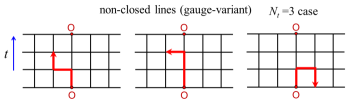
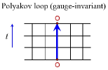
Figure 1: Examples of the trajectories stemming from $I={\rm Tr}_{c,\gamma}(\hat{U}_{4}\hat{\not\!\!D}^{N_{t}-1})$. For each trajectory, the total length is $N_{t}$, and the “first step” is positive temporal direction, $\hat{U}_{4}$. All the trajectories with the odd length $N_{t}$ cannot form a closed loop on the square lattice, so that they are gauge-variant and give no contribution, except for the Polyakov loop. Thus, only the Polyakov-loop component survives in $\langle I\rangle$.

Thus, we obtain the analytical relation between the Polyakov loop $\langle L_{P}\rangle$ and the Dirac modes in QCD on the temporally odd-number lattice [2, 4],

$$\langle L_{P}\rangle=-\frac{(2i)^{N_{t}-1}}{4N_{c}V}\left\langle\sum_{n}\lambda_{n}^{N_{t}-1}\langle n|\hat{U}_{4}|n\rangle\right\rangle_{\rm gauge~{}ave.},$$ (6)

which is mathematically valid in both confined and deconfined phases. From Eq.(6), we can investigate each Dirac-mode contribution to the Polyakov loop. Remarkably, due to the factor $\lambda_{n}^{N_{t}-1}$ in Eq.(6), low-lying Dirac modes gives negligible contribution to the Polyakov loop [2, 4]. In lattice QCD simulations, we have numerically confirmed the relation (6) and scarce contribution of low-lying Dirac modes to the Polyakov loop in both confined and deconfined phases [2].

4 Polyakov-loop fluctuations and Dirac eigenmodes

Next, we consider the Polyakov-loop fluctuations, which can be a good indicator of the QCD transition [5]. On the temporally odd lattice, we derive Dirac-mode expansion formula for Polyakov-loop fluctuations [3], e.g.,

$$R_{A}=\frac{\left\langle\left|\sum\lambda_{n}^{N_{t}-1}\hat{U}_{4}^{nn}\right|^{2}\right\rangle-\left\langle\left|\sum\lambda_{n}^{N_{t}-1}\hat{U}_{4}^{nn}\right|\right\rangle^{2}}{\left\langle\left(\sum\lambda_{n}^{N_{t}-1}{\rm Re}\left(\mathrm{e}^{2\pi ki/3}\hat{U}_{4}^{nn}\right)\right)^{2}\right\rangle-\left\langle\sum\lambda_{n}^{N_{t}-1}{\rm Re}\left(\mathrm{e}^{2\pi ki/3}\hat{U}_{4}^{nn}\right)\right\rangle^{2}},$$ (7)

where $\hat{U}_{4}^{nn}\equiv\langle n|\hat{U}_{4}|n\rangle$, and $k$ is chosen such that the transformed Polyakov loop lies in its real sector [3, 5]. The damping factor $\lambda_{n}^{N_{t}-1}$ appears in the Dirac-mode sum. By removing low-lying Dirac modes, the quark condensate rapidly reduces, but the Polyakov-loop fluctuation is almost unchanged [3].

5 The Wilson loop and Dirac modes on arbitrary square lattices

In this section, we investigate the string tension and the Dirac modes, using the Wilson loop on $R\times T$ rectangle on arbitrary square lattices with any number of $N_{t}$ [4]. The Wilson loop is expressed by the functional trace,

$$W\equiv{\rm Tr}_{c}\hat{U}_{1}^{R}\hat{U}_{-4}^{T}\hat{U}_{-1}^{R}\hat{U}_{4}^{T}={\rm Tr}_{c}\hat{U}_{\rm staple}\hat{U}_{4}^{T},\quad\hat{U}_{\rm staple}\equiv\hat{U}_{1}^{R}\hat{U}_{-4}^{T}\hat{U}_{-1}^{R}.$$ (8)

For even $T$ (odd $T$ case is similar [4]), we consider the functional trace,

$$J\equiv{\rm Tr}_{c,\gamma}\hat{U}_{\rm staple}\hat{\not\!\!D}^{T}=\sum_{n}\langle n|\hat{U}_{\rm staple}{\not\!\!D}^{T}|n\rangle=(-)^{\frac{T}{2}}\sum_{n}\lambda_{n}^{T}\langle n|\hat{U}_{\rm staple}|n\rangle.~{}$$ (9)

Similarly in Sec. 3, one can derive $\langle W\rangle=\frac{(-)^{\frac{T}{2}}2^{T}}{4}\left\langle\sum_{n}\lambda_{n}^{T}\langle n|\hat{U}_{\rm staple}|n\rangle\right\rangle$ [4]. Then, the string tension $\sigma$ is expressed as

$$\sigma=-\lim_{R,T\to\infty}\frac{1}{RT}{\rm ln}\langle W\rangle=-\lim_{R,T\to\infty}\frac{1}{RT}{\rm ln}\left|\left\langle\sum_{n}(2\lambda_{n})^{T}\langle n|\hat{U}_{\rm staple}|n\rangle\right\rangle\right|.~{}~{}$$ (10)

Because of the factor $\lambda_{n}^{T}$ in the sum, the string tension $\sigma$ (the confining force) is to be unchanged by the removal of the low-lying Dirac-mode contribution.

6 The Polyakov loop and Wilson/clover/domain-wall fermions

Finally, we express the Polyakov loop with the eigenmodes of the Wilson, the clover ($O(a)$-improved Wilson) and the domain-wall fermion kernels, where light doublers are absent [1]. The clover fermion kernel is given as

$$\hat{K}=\frac{1}{2a}\sum_{\mu=1}^{4}\gamma_{\mu}(\hat{U}_{\mu}-\hat{U}_{-\mu})+\frac{r}{2a}\sum_{\mu=\pm 1}^{\pm 4}\gamma_{\mu}(\hat{U}_{\mu}-1)+m+\frac{arg}{2}\sigma_{\mu\nu}G_{\mu\nu},$$ (11)

which becomes the Wilson fermion kernel without the last term in RHS. We define eigenmodes and eigenvalues of $\hat{K}$ as $\hat{K}|n\rangle\rangle=i\tilde{\lambda}_{n}|n\rangle\rangle$ with $\tilde{\lambda}_{n}\in{\bf C}$.

We adopt the lattice with $N_{t}=4l+1$, and consider the functional trace,

$$J\equiv\Tr(\hat{U}_{4}^{2l+1}\hat{K}^{2l})=\sum_{n}\langle\langle n|\hat{U}_{4}^{2l+1}{\hat{K}}^{2l}|n\rangle\rangle=\sum_{n}(i\tilde{\lambda}_{n})^{2l}\langle\langle n|\hat{U}_{4}^{2l+1}|n\rangle\rangle.$$ (12)

Since the kernel $\hat{K}$ in Eq. (11) includes many terms, $J\equiv\Tr(\hat{U}_{4}^{2l+1}\hat{K}^{2l})$ consists of products of link-variable operators. In each product, the total number of $\hat{U}$ does not exceed $N_{t}$. Each product gives a trajectory as Fig. 2.

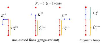
Figure 2: Some examples of the trajectories in $J\equiv\Tr(\hat{U}_{4}^{2l+1}\hat{K}^{2l})$. The length does not exceed $N_{t}$. Only the Polyakov loop can form a closed loop and survives in $\langle J\rangle$.

Among the trajectories, however, only the Polyakov loop can form a closed loop and survives in $\langle J\rangle$, and we derive

$$\langle L_{P}\rangle\propto\langle\sum_{n}\tilde{\lambda}_{n}^{2l}\langle\langle n|\hat{U}_{4}^{2l+1}|n\rangle\rangle~{}\rangle_{\rm gauge~{}ave.}.$$ (13)

Due to $\tilde{\lambda}_{n}^{2l}$, one finds small contribution from low-lying modes of $\hat{K}$ to the Polyakov loop. We also derive a similar formula for the domain-wall fermion.

7 Summary

We have derived relations between the Dirac modes and the confinement quantities (the Polyakov loop, its fluctuations and the string tension) and have found scarce contribution from the low-lying Dirac modes. This indicates some independence of confinement from chiral properties in QCD.