textcolor 0.5 -90 current page.center 0.35 1.8 to report a bug pls visit https://github.com/weinbe58/QuSpin/issues

QuSpin: a Python Package for Dynamics and Exact Diagonalisation of Quantum Many Body Systems.
Part I: spin chains

Abstract

We present a new open-source Python package for exact diagonalization and quantum dynamics of spin(-photon) chains, called QuSpin, supporting the use of various symmetries in 1-dimension and (imaginary) time evolution for chains up to 32 sites in length. The package is well-suited to study, among others, quantum quenches at finite and infinite times, the Eigenstate Thermalisation hypothesis, many-body localisation and other dynamical phase transitions, periodically-driven (Floquet) systems, adiabatic and counter-diabatic ramps, and spin-photon interactions. Moreover, QuSpin’s user-friendly interface can easily be used in combination with other Python packages which makes it amenable to a high-level customisation. We explain how to use QuSpin using four detailed examples: (i) Standard exact diagonalisation of XXZ chain (ii) adiabatic ramping of parameters in the many-body localised XXZ model, (iii) heating in the periodically-driven transverse-field Ising model in a parallel field, and (iv) quantised light-atom interactions: recovering the periodically-driven atom in the semi-classical limit of a static Hamiltonian.

 

Contents

1. 1 What Problems can I Solve with QuSpin?
2. 2 How do I use QuSpin?
   1. 2.1 Exact Diagonalisation of Spin Hamiltonians
   2. 2.2 Adiabatic Control of Parameters in Many-Body Localised Phases
   3. 2.3 Heating in Periodically Driven Spin Chains
   4. 2.4 Quantised Light-Atom Interactions in the Semi-classical Limit: Recovering the Periodically Driven Atom
3. 3 Future Perspectives for QuSpin
4. A Installation Guide in a Few Steps
   1. A.1 Mac OS X/Linux
   2. A.2 Windows
5. B Basic Use of Command Line to Run Python
   1. B.1 Mac OS X/Linux
   2. B.2 Windows
   3. B.3 Execute Python Script (any operating system)
6. C Complete Example Codes
7. D Package Documentation

 

1 What Problems can I Solve with QuSpin?

The study of quantum many-body dynamics comprises a variety of problems, such as dynamical phase transitions (e.g. many-body localisation), thermalising time evolution, adiabatic change of parameters, periodically-driven systems, and many others. In contrast to the tremendous progress made in studying low-energy phenomena based on well-developed sophisticated techniques, such as Quantum Monte Carlo methods [1, 2, 3], Density Matrix Renormalisation Group [4, 5], Matrix Product States [6], Dynamical Mean-Field Theory [7, 8, 9], etc., one of the most popular “cutting-edge” investigation technique for out-of-equilibrium quantum many-body problems remains ‘old school’ exact diagonalisation (ED).

Over the last years, there have appeared freely accessible numerical packages and libraries which contribute to widespread the use of such numerical techniques among the condensed matter community: the Algorithms and Libraries for Physics Simulations [10, 11, 12, 13] (ALPS), C++ libraries for tensor networks: ITensor [14] and Tensor Network Theory Library[15], the Quantum Toolbox in Python (QuTiP) [16, 17], as well as the Mathematica Quantum Many-Body Physics Package DiracQ [18] are among the most common available and freely accessible tools. Although some of these are indeed freely accessible, not all of them are considered open-source as they have certain restrictions about the use and/or distribution of the source code. On the other hand, some members of the scientific community have been pushing for more open-source software, notably in the development of Python. The authors benefited greatly from the community development of these powerful numerical tools and so in the same spirit we present in this paper, an optimised open-source Python package for dynamics and exact diagonalisation of quantum many-body spin systems, called QuSpin:

• A major representative feature of QuSpin is the construction of spin Hamiltonians containing arbitrary (possibly non-local in space) many-body operators. One example is the four-spin operator $\mathcal{O}=\sum_{j}\sigma^{z}_{j}\sigma^{+}_{j+1}\sigma^{-}_{j+2}\sigma^{z}_{j+3}+\mathrm{h.c.}$. Such multi-spin operators are often times generated by the nested commutators typically appearing in higher-order terms of perturbative expansions, such as the Schrieffer-Wolff transformation [19, 20, 21] and the inverse-frequency expansion [22, 23]. Sometimes they appear in the study of exactly solvable reverse-engineered models.

• Another important feature is the availability to use symmetries which, if present in a given model, give rise to conservation laws leading to selection rules between the many-body states. As a result, the Hilbert space reduces to a tensor product of the Hilbert spaces corresponding to the underlying symmetry blocks. Consequently, the presence of symmetries effectively diminishes the relevant Hilbert space dimension which, in turn, allows one to study larger systems. Currently, QuSpin supports the following spin chain symmetries:

  • total magnetisation (particle number in the case of hard-core bosons)

  • parity (i.e. reflection w.r.t. the middle of the chain)

  • spin inversion (on the entire chain but also individually for sublattices $A$ and $B$)

  • the joint application of parity and spin inversion (present e.g. when studying staggered or linear external potentials)

  • translation symmetry

  • all physically meaningful combinations of the above

  We shall see in Sec. 2, constructing Hamiltonians with given symmetries is done by specifying the desired combination of symmetry blocks.

• As of present date, ED methods represent one of the most reliable ways to safely study the dynamics of a generic quantum many-body system. In this respect, it is important to emphasise that with QuSpin the user can build arbitrary time-dependent Hamiltonians. The package contains built-in routines to calculate the real (and imaginary) time evolution of any quantum state under a user-defined time-dependent Hamiltonian based on SciPy’s integration tool for ordinary differential equations [24].

• Besides spin chains, QuSpin also allows the user to couple an arbitrary interacting spin chain to a single photon mode (i.e. quantum harmonic oscillator). In this case, the total magnetisation symmetry is replaced by the combined total photon and spin number conservation. Such an example is discussed in Sec. 2.4.

• Last but not least, QuSpin has been especially designed to construct particularly short and efficient ED codes (typically less than $200$ lines, as we explicitly demonstrate in Sec. 2 and App. C). This greatly reduces the amount of time required to start a new study; it also allows users with little-to-no programming experience to do state-of-the-art ED calculations.

Examples of ‘hot’ problems that can be studied with the help of QuSpin include:

• quantum quenches and quantum dynamics at finite and infinite times

• adiabatic and counter-diabatic ramps

• periodically driven (Floquet) systems

• many-body localisation, Eigenstate Thermalisation hypothesis

• quantum information

• quantised spin-photon interactions and similar cavity QED related models

• dynamical phase transitions and critical phenomena

• machine learning with quantum many-body systems

This list is far from being complete, but it can serve as a useful guideline to the interested user.

Overall, we believe QuSpin to be of particular interest to both students and senior researchers, who can use it to quickly test new exciting ideas, and build up intuition about quantum many-body problems.

2 How do I use QuSpin?

One of the main advantages of QuSpin is its user-friendly interface. To demonstrate how the package works, we shall guide the reader step by step through a short snippets of Python code. In case the reader is unfamiliar with Python, we kindly invite them to accept the challenge of learning the Python basics, while enjoying the study of quantum many-body dynamics, see App. B.

Installing QuSpin is quick and efficient; just follow the steps outlined in App. A.

Below, we stick to the following general guidelines: first, we define the problem containing the physical quantities of interest and show their behaviour in a few figures. After that, we present the QuSpin code used to generate them, broken up into its building blocks. We explain each step in great detail. The complete code, including the lines used to generate the figures shown below, is available in App. C. It is not our purpose in this paper to discuss in detail the interesting underlying physics of these systems; instead, we focus on setting up the Python code to study them with the help of QuSpin, and leave the interested reader figure out the physics details themselves.

2.1 Exact Diagonalisation of Spin Hamiltonians

Physics Setup—Before we show how QuSpin can be used to solve more sophisticated time-dependent problems, let us discuss how to set up and diagonalise static spin chain Hamiltonians. We focus here on the XXZ model in an magnetic field

$$H=\sum_{j=0}^{L-2}\frac{J_{xy}}{2}\left(S^{+}_{j+1}S^{-}_{j}+\mathrm{h.c.}\right)+J_{zz}S^{z}_{j+1}S^{z}_{j}+h_{z}\sum_{j=0}^{L-1}S^{z}_{j},$$ (1)

where $J_{xy}$ and $J_{zz}$ are the $xy$- and $zz$-interaction strengths, respectively, and $h_{z}$ is the external field along the $z$ direction. Note that we enumerate the $L$ sites of the chain by $j=0,1,\dots,L-1$ to conform with Python’s array indexing convention. We shall assume open boundary conditions.

Code Analysis—Let us now build and diagonalise $H$ using QuSpin. First, we load the required Python packages. Note that we adopt the commonly used abbreviation for NumPy, np.

Next, we define the physical model parameters. In doing so, it is advisable to use the floating point when the coupling is meant to be a non-integer real number, in order to avoid problems with division: for example, 1 is the integer $1$ while 1.0 – the corresponding float. For instance, in Python 2.7, we have 0.5$\neq$1/2$=$0, but rather 0.5$=$1.0/2.0.

To set up any Hamiltonian, we need to calculate the basis of the Hilbert space it is defined on, see line 13 below. Note that, since we work with spin operators here, it is required to pass the flag pauli=False; failure to do so will result in a Hamiltonian defined in terms of the Pauli spin matrices $\sigma^{\mu}_{i}=2S^{\mu}_{i}$. One can also display the basis using the command print basis.

The XXZ Hamiltonian $H$ from Eq. (1) obeys certain symmetries. In particular, one can specify a magnetisation sector (a.k.a. filling) using the basis optional argument N_up=int, where int$\in[0,L]$ is any integer to specify the number of up-spins, see line 14. However, magnetisation is not the only integral of motion – the model also conserves parity, i.e. reflection w.r.t. the middle of the chain. The parity operator has eigenvalues $\pm 1$ and thus further divides the Hilbert space into two new subspaces. To restrict the Hamiltonian to either one of them, we use the basis optional argument pblock=$\pm 1$. Since parity and magnetisation commute, it is also possible to request them simultaneously, see line 15. We stress that each one of the lines 13-15 is sufficient to build the basis on its own and we only show them all here for clarity.

In QuSpin, many-body operators $JS_{i_{1}}^{\mu_{1}}\dots S_{i_{n}}^{\mu_{n}}$ are defined by a string of letters $\mu_{1},\dots\mu_{n}$, representing the operator types, $\mu_{i}\in$["+","-","x","y","z"], together with a site-coupling list $[J,i_{1},\dots,i_{n}]$ which holds the coupling and the indices for the sites $i$ that each spin operator acts at on the lattice. Setting up the spin-spin operators in the XXZ model goes as follows. First, we need to define the site-coupling lists J_zz, J_xy and h_z. To uniquely specify a two-spin interaction, we need (i) the coupling, and (ii) – the labels of the sites the two operators act on. QuSpin uses Python’s indexing convention meaning that the first lattice site is always $i=0$, and the last one: $i=L-1$. For example, for the $zz$-interaction, the coupling is Jzz, while the two sites are the nearest neighbours i,i+1. Hence, the list [Jzz,i,i+1] defines the bond operator $J_{zz}(0)S^{\mu}_{i}S^{\nu}_{i+1}$ (we specify $\mu$ and $\nu$ in the next step). To define the total interaction energy $J_{zz}(0)\sum_{i=0}^{L-2}S^{\mu}_{i}S^{\nu}_{i+1}$, all we need is to loop over the $L-2$ bonds of the open chain. In the same spirit one can define boundary or single-site operators, such as h_z. It is also possible to set up multi-spin operators, as we show in Sec. 2.3.

The above lines of code specify the coupling but not yet which spin operators are being coupled. i.e. we have not yet fixed $\mu$ and $\nu$. To do this, we need to create a static and/or dynamic operator list. As the name suggests, static lists define time-independent operators. Given the site-coupling list J_xy from above, it is easy to define the operator $J_{xy}/2\sum_{i=0}^{L-2}S^{+}_{i}S^{-}_{i+1}$ by specifying the spin operator type in the same order as the site indices appear in the corresponding site-coupling list: [["+-",J_xy]]. In other words, the order "+-" corresponds directly to the site-index order "i,i+1". Similarly, one should set up the hermitian conjugate term $J_{xy}/2\sum_{i=0}^{L-2}S^{-}_{i}S^{+}_{i+1}$ as [["-+",J_xy]]. In the end, one can concatenate these operator lists to produce the static part of the Hamiltonian.

If the Hamiltonian has time dependence, it is defined using dynamic lists. Since we are dealing with a static problem in this section, we set the dynamic to an empty list. In the following three sections, we show how to set up non-trivial time-dependent Hamiltonians.

Once the static and dynamic lists are set up, building up the corresponding Hamiltonian is a one-liner. In QuSpin, this is done using the hamiltonian constructor class, see line 24 below. The first required argument is the static list, while the second one – the dynamic list. These two arguments must appear in this order. Another argument is the basis, which carries the necessary information about symmetries. Yet whether a given Hamiltonian has these symmetries, depends on the operators defined in the static and dynamic lists. The hamiltonian class performs an automatic check on the Hamiltonian for hermiticity, the presence of magnetisation conservation and other requested symmetries, and raises an error if these checks fail.

Having set up the Hamiltonian, we now briefly discuss a few ED routines. If one is only interested in the spectrum E, one can obtain it as follows:

If, on top, one also needs the unitary matrix V with the corresponding eigenvectors in its columns, the proper command is

Often times, one does not need to fully diagonalise $H$, but a part of the spectrum suffices. For instance, if one is interested in the many-body bandwidth of the model, it can be computed from the smallest and largest eigenvalues. This can be done efficiently using the eigsh attribute (eigenvalues of a sparse hermitian matrix), see line 32 below. The optional argument k=2 ensures that only two eigenstates are calculated. To determine which ones, the argument which="BE" specifies them to be the two states at Both Ends of the spectrum. Convergence of the underlying diagonalisation algorithm is enforced by explicitly specifying the number of maximal iterations: maxiter=1E4. If we do not want the eigenstates returned, we use return_eigenvectors=False.

Last, we show how to find that eigenenergy and eigenstate, closest to a given predefined energy E_star. This is also done using the eigsh attribute. Since we request only one state, we set k=1. The predefined energy is then passed using the optional argument sigma. More on how eigsh works can be found in the SciPy online documentation.

The entire code is available in Example Code 1.

2.2 Adiabatic Control of Parameters in Many-Body Localised Phases

Physics Setup—Strongly disordered many-body models have recently enjoyed a lot of attention in the theoretical condensed matter community. It has been shown that, beyond a critical disorder strength, these models undergo a dynamical phase transition from an delocalised ergodic (thermalising) phase to a many-body localised (MBL), i.e. non-conducting, non-thermalising phase, in which the system violates the Eigenstate Thermalisation hypothesis [25, 26, 27, 28, 29, 30, 31].

In our first QuSpin example, we show how one can study the adiabatic control of model parameters in many-body localised phases. It was recently argued that the adiabatic theorem does not apply to disordered systems [32]. On the other hand, controlling the system parameters in MBL phases is of crucial experimental[33, 34, 35, 36, 37] significance. Thus, the question as to whether there exists an adiabatic window for some, possibly intermediate, ramp speeds (as is the case for periodically-driven systems[38]), is of particular and increasing importance.

Let us consider the XXZ open chain in a disordered $z$-field with the time-dependent Hamiltonian

$$H(t) = \sum_{j=0}^{L-2}\frac{J_{xy}}{2}\left(S^{+}_{j+1}S^{-}_{j}+\mathrm{h.c.}\right)+J_{zz}(t)S^{z}_{j+1}S^{z}_{j}+\sum_{j=0}^{L-1}h_{j}S^{z}_{j},$$

$$J_{zz}(t) = (1/2+vt)J_{zz}(0),$$ (2)

where $J_{xy}$ is the spin-spin interaction in the $xy$-plane, disorder is modelled by a uniformly distributed random field $h_{j}\in[-h_{0},h_{0}]$ of strength $h_{0}$ along the $z$-direction, and the spin-spin interaction along the $z$-direction – $J_{zz}(t)$ – is the adiabatically-modulated (ramp) parameter. In the following, we set $J_{zz}(0)=1$ as the energy unit. It has been demonstrated that this model exhibits a transition to an MBL phase [39]. In particular, for $h_{0}=h_{\mathrm{MBL}}=3.72$ the system is in a many-body localised phase, while for $h_{0}=h_{\mathrm{ETH}}=0.1$ the system is in the ergodic (ETH) delocalised phase. We now choose the ramp protocol $J_{zz}(t)=(1/2+vt)J_{zz}(0)$ with the ramp speed $v$, and evolve the system with the Hamiltonian $H(t)$ from $t_{i}=0$ to $t_{f}=(2v)^{-1}$. We choose the initial state $|\psi_{i}\rangle=|\psi(t_{i})\rangle$ from the middle of the spectrum of $H(t_{i})$ to ensure typicality; more specifically we choose $|\psi_{i}\rangle$ to be that eigenstate of $H(t_{i})$ whose energy is closest to the middle of the spectrum of $H(t_{i})$, where the density of states, and thus the thermodynamic entropy, is largest.

To determine whether the system can adiabatically follow the ramp, we use two different indicators: (i) we evolve the state up to time $t_{f}$ and project it onto the eigenstates of $H(t_{f})$. The corresponding diagonal entropy density:

$$s_{d}=-\frac{1}{L}\mathrm{tr}\left[\rho_{d}\log\rho_{d}\right],\qquad\rho_{d}=\sum_{n}|\langle n|\psi(t_{f})\rangle|^{2}|n_{f}\rangle\langle n_{f}|$$ (3)

in the basis $\{|n_{f}\rangle\}$ of $H(t_{f})$ at small enough ramp speeds $v$, is a measure of the delocalisation of the time-evolved state $\psi(t_{f})\rangle$ among the energy eigenstates of $H(t_{f})$. If, for instance, after the ramp the system still occupies a single eigenstate $|\tilde{n}_{f}\rangle$, then $s_{d}=0$.

The second measure of adiabaticity we use is (ii) the entanglement entropy density

$$s_{\mathrm{ent}}(t_{f})=-\frac{1}{|\mathrm{A}|}\mathrm{tr}_{\mathrm{A}}\left[\rho_{\mathrm{A}}(t_{f})\log\rho_{\mathrm{A}}(t_{f})\right],\qquad\rho_{\mathrm{A}}(t_{f})=\mathrm{tr}_{\mathrm{A^{c}}}|\psi(t_{f})\rangle\langle\psi(t_{f})|$$ (4)

of subsystem A, defined to contain the left half of the chain and $|\mathrm{A}|=L/2$. We denoted the reduced density matrix of subsystem A by $\rho_{\mathrm{A}}$, and $\mathrm{A^{c}}$ is the complement of A.

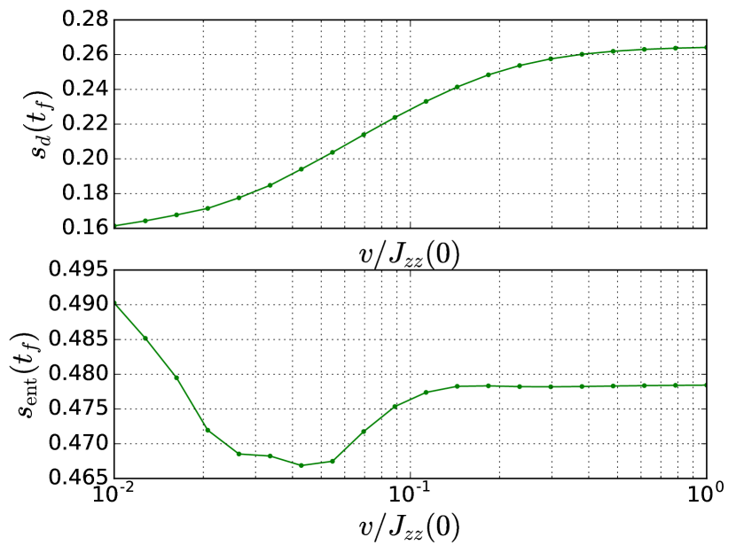
(a) ETH phase

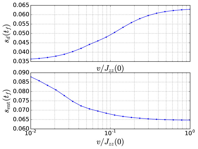
(b) MBL phase

Figure 1: Diagonal and entanglement entropy densities as a function of the ramp speed in the MBL and delocalised (ETH) phases of the ramped disordered XXZ model. The ramped protocol is chosen as $J_{zz}(t)=(1/2+vt)J_{zz}(0)$. The parameters are $J_{xy}/J_{zz}(0)=1.0$, $h_{\mathrm{MBL}}/J_{zz}(0)=3.9$, $h_{\mathrm{ETH}}/J_{zz}(0)=0.1$, and $L=10$. Disorder averaging was performed over $1000$ realisations.

Figure 1 shows the entropies vs. ramp speed in the MBL and ETH phases. The interesting underlying physics is, however, beyond the purpose of this paper.

Code Analysis—Let us now explain how one can study this problem numerically using QuSpin. We begin by first loading the required Python packages.

Since we want to produce many realisations of the data and average over disorder, we specify the simulations parameters: n_real is the number of disorder realisations, while n_jobs is the joblib parallelisation parameter which determines how many Python processes to run simultaneously.

Next, we define the physical model parameters.

The time-dependent disordered Hamiltonian consists of two parts: the time-dependent XXZ model which is disorder-free, and the disorder field whose values differ from one realisation to another. We focus on the XXZ part first. Let us code up the driving protocol $J_{zz}(t)=(1/2+vt)J_{zz}(0)$. As already explained, our goal is to obtain the disorder-averaged entropies as a function of the ramp speed $v$. Hence, for each disorder realisation, we need to evolve the initial state many times, each corresponding to a different ramp speed. However, calculating the Hamiltonian every single time is not particularly efficient from the point of view of simulation runtime. We thus want to set up a family of Hamiltonians $\{v:H(t;v)\}$ at once, and we shall employ Python’s features to do so. This will require that the drive speed v is not a parameter of the function ramp, see line 29, but is declared beforehand as a global variable. Once, ramp has been defined, reassigning v dynamically induces the corresponding change in ramp without any need to re-define ramp itself. We shall comment on how this works later on in the code.

To set up the static part of the Hamiltonian, we follow the same steps as in Sec. 2.1. Since the Hamiltonian (2) conserves the total magnetisation, the overlap betweens states of different magnetisation sectors vanishes trivially, and we can reach larger system sizes by working in a fixed magnetisation sector. A natural choice is the zero-magnetisation sector which contains the ground state. Parity is broken by the disorder field, so we leave it out.

The time-dependent part of the Hamiltonian is defined using dynamic lists. Similar to their static counterparts, one needs to define an operator string, say "zz" to declare the specific operator from a site-coupling list. Apart from the site-coupling list J_zz, however, a dynamic list also requires a time-dependent function and its arguments, see line 34 below. In the linearly driven XXZ-Hamiltonian we are setting up here, the function arguments ramp_args is an empty list, see line 31 above. The careful reader might have noticed that there is a certain freedom in coding the coupling of the time-dependent term, $J_{zz}(t)=(1/2+vt)J_{zz}(0)$: here we choose to include the constant Jzz_0 in the zz site-coupling list and hence this factor is absent in the definition of the ramp function. Building the Hamiltonian is straightforward, as we explained in Sec. 2.1.

To produce the entropies vs. ramp speed data over many disorder realisations, we define the function realization which returns a two NumPy arrays for the MBL and ETH phases respectively. Each array contains values of the values of the diagonal entropy density $s_{d}$, and the values of the entanglement entropy density $s_{\mathrm{ent}}$ for each velocity, as columns of the array. We now walk the reader step by step through the definition of realization. The first argument is the vector of ramp speeds, vs, required for the dynamics. The second argument is the time-dependent XXZ Hamiltonian H_XXZ to which we shall be adding a disordered $z$-field for each disorder realisation. The third argument is the spin basis which is required to calculate $s_{\mathrm{ent}}$. The fourth (last) argument is the realisation number, which is only used to print a message about the duration of the single realisation run.

We time each realisation simulation, using the package time:

In order to properly be able to use $H_{\mathrm{XXZ}}(t;v)$ as a family of Hamiltonians in $v$ (we shall see exactly how this works in a moment), we explicitly declare the variable v global.

Since the problem involves disorder, we have to generate multiple disorder realisations. In this case, it is recommended to reset the pseudo-random number generator before any random numbers have been drawn. This is because the code spawns multiple python processes to do the disorder realization in parallel. Therefore, if the pseudo-random number generator is seeded before the new processes are spawned, all the parallel jobs will produce the same disorder realizations.

Next, we set up the full disordered time-dependent Hamiltonian of the problem $H(t)=H_{\mathrm{XXZ}}(t)+\sum_{j}h_{j}S^{z}_{j}$. The random field $h_{j}$ differs from one realisation to another and is, therefore, defined inside the realization function. Recall that we want to compare the localised with the delocalised regimes, corresponding to the disorder strengths $h_{\mathrm{MBL}}$ and $h_{\mathrm{ETH}}$, respectively. For each lattice site $i$ we draw a random number unscaled_fields[i] uniformly in the interval $[-1,1]$, and store it in the vector unscaled_fields, see line 55 below. Building the external $z$-field proceeds in exactly the same way as before: (i) we calculate the site-coupling list, line 57, (ii) we designate that the operator is along the $z$-axis by defining a static operator list, line 59, and (iii) we use the already computed spin basis to construct the operator matrix with the hamiltonian class, lines 61-62. QuSpin has the option to disable the default checks on hermiticity, magnetisation (particle number) conservation, and symmetries using the auxiliary dictionary no_checks passed straight to hamiltonian as keyword arguments. This can allow the user to define non-hermitian operators. Last, in lines 64-65, we define the MBL and ETH time-dependent Hamiltonians, corresponding to the two disorder strengths $h_{\mathrm{ETH}}$ and $h_{MBL}$.

Let us first focus on the MBL phase. We want the initial state to be as close as possible to an infinite-temperature state within the given symmetry sector. To this end, we can first calculate the minimum and maximum energy, Emin and Emax of the spectrum of $H_{\mathrm{MBL}}(t=0)$. Then, by taking the ‘centre-of-mass’ we obtain a number, E_inf_temp, which represents the infinite-temperature energy up to finite-size effects, line 72. Note that the **eigsh_args is a standard Python way of reading off the arguments by name from a dictionary.

The initial state psi_0 is then that eigenstate of $H_{\mathrm{MBL}}(t=0)$, whose energy is closest to E_inf_temp, using optional argument sigma=E_inf_temp.

The calculation of the diagonal entropy density $s_{d}$ requires the eigensystem of the Hamiltonian $H_{\mathrm{MBL}}(t_{f})$ at the end of the ramp $t_{f}=(2v_{f})^{-2}$. The entire spectrum and the corresponding eigenstates are obtained using the hamiltonian method eigh. For time-dependent Hamiltonians, eigh accepts the argument time to specify the time slice. Unless explicitly specified, time=0.0 by default. Note that we re-set the ramp speed v to unity to calculate the correct eigensystem of the Hamiltonian at the end of the ramp, since $v$ a parameter of $H(t;v)$ (see line 68).

To calculate the entropies for each ramp speed, we use the helper function _do_ramp (defined below), which first evolves the initial state according to the $v$-dependent Hamiltonian $H_{\mathrm{MBL}}(t;v)$ for a fixed ramp speed $v$. In line 78 we loop over the ramp speed vector vs. More importantly, however, the iteration index v carries the same name as the parameter in the drive function ramp. Thus, every time a new ramp speed is read off the vector vs, the external parameter v changes its value. Because v is a global variable, this change induces a change into the function ramp which, in turn, induces a change in the dynamic list. Thus, at the end of the day, a new member of the family of MBL Hamiltonians, $\{v:H_{\mathrm{MBL}}(t;v)\}$, is picked and parsed to _do_ramp to do the time evolution with. Hence, we end up with a convenient and automatic way of generating the whole family $\{v:H_{\mathrm{MBL}}(t;v)\}$, while having to calculate the operators in the Hamiltonian only once.

It remains to discuss the helper function _do_ramp. Its job is to evolve the initial state psi_0 with the hamiltonian object H and to calculate the entropies at the end of the ramp.

Given a ramp speed v, we first determine the total ramp time t_f. Evolving a quantum state under any Hamiltonian H is easily done with the hamiltonian method evolve, see line 114. evolve requires the initial state psi_0, the starting time – here 0.0, and a vector of times to return the evolved state at, but since we are only interested in the state at the final time – we pass the final time t_f. The evolve method has further interesting features which we discuss in Secs. 2.3 and 2.4.

Once we have the state at the end of the ramp, we can obtain the entropies as follows. Calculating $s_{\mathrm{ent}}$ is done using the measurements function ent_entropy which we imported in line 3. It requires the quantum state (here the pure state psi), and the basis the state is stored in. Optionally, one can specify the site indices which define the subsystem retained after the partial trace using the argument chain_subsys. Note that ent_entropy returns a dictionary, in which the value of the entanglement entropy is stored under the key "Sent". The function ent_entropy has a many further features, described in the documentation, see App. D.

Similarly, there is a built-in function to calculate the diagonal entropy density $s_{d}$ of a state psi in a given basis (here V_final), called diag_ensemble. This function can calculate a variety of interesting quantities in the diagonal ensemble defined by the eigensystem arguments (here E_final, V_final). We again invite the interested reader to check out the documentation in App. D.

This concludes the definition of _do_ramp.

Back to the function realization, we have already seen how to obtain the entropies in the MBL phase. We now do the same thing in the delocalised ETH phase. The code is the same as the MBL one:

We can now display how long the single iteration took

and conclude the definition of realization:

Now that we have written the realization function, we can call it n_real times to produce the data. The easiest way of doing this is to loop over the disorder realisation, as shown in lines 126-129. However, a better to proceed makes use of the joblib package which can distribute simultaneous function calls over n_job Python processes, see line 130^,. To learn more about how this works, we invite the readers to check the documentation of joblib. Having produced and extracted the entropy vs. ramp speed data, we are ready to perform the disorder average by taking the mean over all realisations, lines 133-135.

The complete code including the lines that produce Fig. 1 is available in Example Code 2.

2.3 Heating in Periodically Driven Spin Chains

Physics Setup—As a second example, we now show how one can easily study heating in the periodically-driven transverse-field Ising model with a parallel field [40, 41, 42]. This model is non-integrable even without the time-dependent driving protocol. The time-periodic Hamiltonian is defined as a two-step protocol as follows:

$$H(t) = \left\{\begin{array}[]{cl}J\sum_{j=0}^{L-1}\sigma^{z}_{j}\sigma^{z}_{j+1}+h\sum_{j=0}^{L-1}\sigma^{z},&t\in[-T/4,\phantom{3}T/4]\\ \kern-80.00012ptg\sum_{j=0}^{L-1}\sigma^{x}_{j},&t\in[\phantom{-}T/4,3T/4]\end{array}\right\}\mathrm{mod}\ T,$$ (7)

$$= \sum_{j=0}^{L-1}\frac{1}{2}\left(J\sigma^{z}_{j}\sigma^{z}_{j+1}+h\sigma^{z}+g\sigma^{x}_{j}\right)+\frac{1}{2}\text{sgn}\left[\cos\Omega t\right]\left(J\sigma^{z}_{j}\sigma^{z}_{j+1}+h\sigma^{z}-g\sigma^{x}_{j}\right).$$ (8)

Unlike the previous example, here we consider a closed spin chain with a periodic boundary (i.e. a ring). The spin-spin interaction strength is denoted by $J$, the transverse field – by $g$, and the parallel field – by $h$. The period of the drive is $T$ and, although the periodic step protocol contains infinitely many Fourier harmonics, we shall refer to $\Omega=2\pi/T$ as the frequency of the drive.

Since the Hamiltonian is periodic, $H(t+T)=H(t)$, Floquet’s theorem applies and postulates that the dynamics of the system at times $lT$, integer multiple of the driving period (a.k.a. stroboscopic times), is governed by the time-independent Floquet Hamiltonian $H_{F}$. In other words, the evolution operator is stroboscopically given by

$$U(lT)=\mathcal{T}_{t}\exp\left(-i\int^{lT}_{0}H(t)\mathrm{d}t\right)=\exp(-ilTH_{F}).$$ (9)

While the Floquet Hamiltonian for this system cannot be calculated analytically, a suitable approximation can be found at high drive frequencies by means of the van Vleck inverse-frequency expansion [22, 43]. However, this expansion is known to calculate the effective Floquet Hamiltonian $H_{\mathrm{eff}}$ in a different basis than the original stroboscopic one:

$$H_{F}=\exp[-iK_{\mathrm{eff}}(0)]H_{\mathrm{eff}}\exp[iK_{\mathrm{eff}}(0)],$$

which requires the additional calculation of the so-called Kick operator $K_{\mathrm{eff}}(0)$ to ‘rotate’ to the original basis.

In the inverse-frequency expansion, we expand both $H_{\mathrm{eff}}$ and $K_{\mathrm{eff}}(0)$ in powers of the inverse frequency. Let us label these approximate objects by the superscript ⁽ⁿ⁾, suggesting that the corresponding operators are of order $\mathcal{O}(\Omega^{-n})$:

$$H_{F} = H_{F}^{(0)}+H_{F}^{(1)}+H_{F}^{(2)}+H_{F}^{(3)}+\mathcal{O}(\Omega^{-4})=H_{F}^{(0+1+2+3)}+\mathcal{O}(\Omega^{-4}),$$

$$H_{\mathrm{eff}} = H_{\mathrm{eff}}^{(0)}+H_{\mathrm{eff}}^{(1)}+H_{\mathrm{eff}}^{(2)}+H_{\mathrm{eff}}^{(3)}+\mathcal{O}(\Omega^{-4}),$$

$$K_{\mathrm{eff}} = K_{\mathrm{eff}}^{(0)}+K_{\mathrm{eff}}^{(1)}+K_{\mathrm{eff}}^{(2)}+K_{\mathrm{eff}}^{(3)}+\mathcal{O}(\Omega^{-4}),$$

Using the short-hand notation one can show that, for this problem, all odd-order terms in the van Vleck expansion vanish [see App. G of Ref. [44]]

$$H_{F}^{(0+1+2+3)}=H_{F}^{(0+2)}\approx\mathrm{e}^{-iK_{\mathrm{eff}}^{(2)}(0)}\left(H_{\mathrm{eff}}^{(0)}+H_{\mathrm{eff}}^{(2)}\right)\mathrm{e}^{+iK_{\mathrm{eff}}^{(2)}(0)},$$ (10)

while the first few even-order ones are given by

$$H_{\mathrm{eff}}^{(0)} = \frac{1}{2}\sum_{j}J\sigma^{z}_{j}\sigma^{z}_{j+1}+h\sigma^{z}_{j}+g\sigma^{x}_{j},$$

$$H_{\mathrm{eff}}^{(2)} = -\frac{\pi^{2}}{12\Omega^{2}}\sum_{j}J^{2}g\sigma^{z}_{j-1}\sigma^{x}_{j}\sigma^{z}_{j+1}+Jgh(\sigma^{x}_{j}\sigma^{z}_{j+1}+\sigma^{z}_{j}\sigma^{x}_{j+1})+Jg^{2}(\sigma^{y}_{j}\sigma^{y}_{j+1}-\sigma^{z}_{j}\sigma^{z}_{j+1})$$

$$\quad\qquad\qquad+\left(J^{2}g+\frac{1}{2}h^{2}g\right)\sigma^{x}_{j}+\frac{1}{2}hg^{2}\sigma^{z}_{j},$$

$$K_{\mathrm{eff}}^{(0)} = {\bf 0},$$

$$K_{\mathrm{eff}}^{(2)}(0) = \frac{\pi^{2}}{8\Omega^{2}}\sum_{j}Jg\left(\sigma^{z}_{j}\sigma^{y}_{j+1}+\sigma^{y}_{j}\sigma^{z}_{j+1}\right)+hg\sigma^{y}_{j},$$ (11)

It was recently argued based on the aforementioned Floquet theorem that, in a closed periodically driven system, stroboscopic dynamics is sufficient to completely quantify heating [45], and we shall make use of this fact in our little study here. We choose as the initial state the ground state of the approximate Hamiltonian $H_{F}^{(0+1+2+3)}$ and denote it by $|\psi_{i}\rangle$:

$$|\psi_{i}\rangle=|\mathrm{GS}(H_{F}^{(0+1+2+3)})\rangle.$$ (12)

Regimes of slow and fast heating can then be easily detected by looking at the energy density $\mathcal{E}$ absorbed by the system from the drive

$$\mathcal{E}(lT)=\frac{1}{L}\langle\psi_{i}|\mathrm{e}^{ilTH_{F}}H_{F}^{(0+1+2)}\mathrm{e}^{-ilTH_{F}}|\psi_{i}\rangle,$$ (13)

and the entanglement entropy of a subsystem. We call this subsystem A and define it to contain $L/2$ consecutive chain sites:

$$s_{\mathrm{ent}}(lT)=-\frac{1}{L_{\mathrm{A}}}\mathrm{tr}_{\mathrm{A}}\left[\rho_{\mathrm{A}}(lT)\log\rho_{\mathrm{A}}(lT)\right],\ \ \mathrm{with}\ \ \rho_{\mathrm{A}}(lT)=\mathrm{tr}_{\mathrm{A^{c}}}\left[\mathrm{e}^{-ilTH_{F}}|\psi_{i}\rangle\langle\psi_{i}|\mathrm{e}^{ilTH_{F}}\right],$$ (14)

where the partial trace in the definition of the reduced density matrix (DM) $\rho_{\mathrm{A}}$ is over the complement of A, denoted $\mathrm{A^{c}}$, and $L_{\mathrm{A}}=L/2$ denotes the length of subsystem A.

Since heating can be exponentially slow at high frequencies [46, 47, 48, 49], one might be interested in calculating also the infinite-time quantities

$$\overline{\mathcal{E}}=\lim_{N\to\infty}\frac{1}{N}\sum_{l=0}^{N}\mathcal{E}(lT),\qquad\overline{s}_{\mathrm{rdm}}=-\frac{1}{L_{\mathrm{A}}}\mathrm{tr}_{\mathrm{A}}\left[\overline{\rho}_{\mathrm{A}}\log\overline{\rho}_{\mathrm{A}}\right],\qquad s_{d}^{F}=-\frac{1}{L}\mathrm{tr}\left[\rho^{F}_{d}\log\rho^{F}_{d}\right],$$ (15)

where $\overline{\rho}_{\mathrm{A}}$ is the infinite-time reduced DM of subsystem A, and $\rho^{F}_{d}$ is the DM of the Diagonal ensemble [50] in the exact Floquet basis $\{|n_{F}\rangle\!\!:H_{F}|n_{F}\rangle=E_{F}|n_{F}\rangle\}$:

$$\overline{\rho}_{\mathrm{A}}=\lim_{N\to\infty}\frac{1}{N}\sum_{l=0}^{N}\rho_{\mathrm{A}}(lT)=\mathrm{tr}_{\mathrm{A^{c}}}\left[\rho_{d}^{F}\right],\qquad\rho_{d}^{F}=\sum_{n}|\langle\psi_{i}|n_{F}\rangle|^{2}|n_{F}\rangle\langle n_{F}|$$

We note in passing that in general $\overline{s}_{\mathrm{rdm}}\neq\lim_{N\to\infty}N^{-1}\sum_{l=0}^{N}s_{\mathrm{ent}}(lT)$ due to interference terms, although the two may happen to be close.

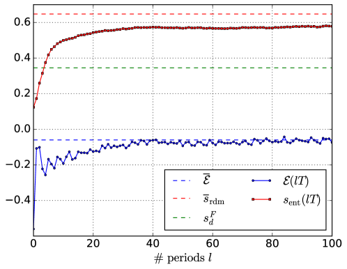
Figure 2: Stroboscopic dynamics of the energy density and entanglement entropy density (solid lines), together with their infinite-time values (dashed lines) in the periodically-driven TFIM in a parallel field. The parameters are $g/J=0.809$, $h/J=0.9045$, $\Omega/J=4.5$, and $L=14$.

In Fig. 2 we show the time evolution of $\mathcal{E}(lT)$ and $s_{\mathrm{ent}}(lT)$ as a function of the number of driving cycles $l$ for a given drive frequency, together with their infinite-time values.

Code Analysis—Let us now discuss the QuSpin code for this problem in detail. First we load the required classes, methods and functions required for the computation:

After that, we define the model parameters:

The time-periodic step drive of frequency Omega can easily be incorporated through the following function:

Next, we define the basis, similar to the example in Sec. 2.2. One can convince oneself that the Hamiltonian in Eq. (7) possesses two symmetries at all times $t$ which are, therefore, also inherited by the Floquet Hamiltonian. These are translation invariance and parity (i.e. reflection w.r.t. the centre of the chain). To incorporate them, one needs to specify the desired block for each symmetry: kblock=int selects the many-body states of total momentum $2\pi/L$*int, while pblock=$\pm 1$ sets the parity sector. For all total momenta different from $0$ and $\pi$, the translation operator does not commute with parity, in which case semi-momentum states producing a real Hamiltonian are the natural choice [51]. The optional argument a=1 specifies the number of sites per unit cell.

The definition of the site-coupling lists proceeds similarly to the MBL example above. It is interesting to note how the periodic boundary condition is encoded in line 25 using the modulo operator %. Compared to open boundaries, the PBC J_nn list now also has a total of L elements, as many as there are sites and bonds on the ring.

To program the full Hamiltonian $H(t)$, we use the second line of Eq. (7). The time-independent part is defined using the static operator list. For the time-dependent part, we need to pass the function drive and its arguments drive_args, defined in lines 15-18, to all operators the drive couples to. In fact, QuSpin is smart enough to automatically sum up all operators multiplied by the same time-dependent function in any dynamic list created. Note that since we are dealing with a Hamiltonian defined by Pauli matrices and not the spin-$1/2$ operators, we drop the optional argument pauli for the hamiltonian class, since by default it is set to pauli=True.

The following lines define the approximate van Vleck Floquet Hamiltonian, cf. Eq. (2.3). Of particular interest is line 37 where we define the site-coupling list for the three-spin operator "zxz". Apart from the coupling J**2*g, we now need to specify the three site indices i,(i+1)%L,(i+2)%L for each of the operators "zxz", respectively. In a similar fashion, one can define any multi-spin operator.

In order to rotate the state from the van Vleck to the stroboscopic (Floquet-Magnus) picture, we also have to calculate the kick operator at time $t=0$. While the procedure is the same as above, note that $K_{\mathrm{eff}}(0)$ has imaginary matrix elements, whence the variable dtype=np.complex128 is used (in fact this is the default dtype optional argument that the hamiltonian class assumes if one does not pass this argument explicitly). If the user tries to force define a real-valued Hamiltonian which, however, has complex matrix elements, QuSpin will raise an error.

Next, we need to find $H_{F}^{(0+2)}=\exp[-iK^{(2)}_{\mathrm{eff}}(0)]H^{(0+2)}_{\mathrm{eff}}\exp[iK^{(2)}_{\mathrm{eff}}(0)]$. To this end, we make use of the hamiltonian class method rotate_by which conveniently provides a function for this purpose. By specifying the optional argument generator=True, rotate_by recognises the operator $B$ as a generator and defines a linear transformation to ‘rotate’ a hamiltonian object $A$ via $\exp(a^{*}B^{\dagger})A\exp(aB)$ for any complex-valued number $a$. Although we do not make use of it directly here, it might also be useful for the user to become familiar with the documentation of the exp_op class which provides the matrix exponential, cf. App. D, and contains a variety of useful method functions. For instance, $\exp(zB)A$ can be obtained using exp_op(B,a=z).dot(A), while $A\exp(zB)$ is A.dot(exp_op(B,a=z)) for any complex number z.

Now that we have concluded the initialisation of the approximate Floquet Hamiltonian, it is time to discuss how to study the dynamics of the system. We start by defining a vector of times t, particularly suitable for the study of periodically driven systems. We initialise this time vector as an object of the Floquet_t_vec class. The arguments we need are the drive frequency Omega, the number of periods (here 100), and the number of time points per period len_T (here set to 1). Once initialised, t has many useful attributes, such as the time values t.vals, the drive period t.T, the stroboscopic times t.strobo.vals, or their indices t.strobo.inds. The Floquet_t_vec class has further useful properties, described in the documentation in App. D.

To calculate the exact stroboscopic Floquet Hamiltonian $H_{F}$, one can conveniently make use of the Floquet class. Currently, it supports three different ways of obtaining the Floquet Hamiltonian: (i) passing an arbitrary time-periodic hamiltonian object it will evolve each Fock state for one period to obtain the evolution operator $U(T)$. This calculation can be parallelised using the Python module joblib, activated by setting the optional argument n_jobs. (ii) one can pass a list of static hamiltonian objects, accompanied by a list of time steps to apply each of these Hamiltonians at. In this case, the Floquet class will make use of the matrix exponential to find $U(T)$. Instead, here we choose, (iii), to use a single dynamic hamiltonian object $H(t)$, accompanied by a list of times $\{t_{i}\}$ to evaluate it at, and a list of time steps $\{\delta t_{i}\}$ to compute the time-ordered matrix exponential as $\prod_{i}\exp(-iH(t_{i})\delta t_{i})$. The Floquet class calculates the quasienergies EF folded in the interval $[-\Omega/2,\Omega/2]$ by default. If required, the user may further request the set of Floquet states by setting VF=True, the Floquet Hamiltonian, HF=True, and/or the Floquet phases – thetaF=True. For more information on Floquet_t_vec, the user is advised to consult the package documentation, see App. D.

As discussed in the setup of the problem, we choose for the initial state the ground state of the approximate Hamiltonian $H_{F}^{(0+2)}$. Following the discussion in Sec. 2.1, we use the hamiltonian class attribute eigsh.

Finally, we can calculate the time-dependence of the energy density $\mathcal{E}(t)$ and the entanglement entropy density $s_{\mathrm{ent}}(t)$. This is done using the measurements function obs_vs_time. If one evolves with a constant Hamiltonian (which is effectively the case for stroboscopic time evolution), QuSpin offers two different but equivalent options, that we now discuss. (i) As a first required argument of obs_vs_time one passes a tuple (psi_i,E,V) with the initial state, the spectrum, and the eigenbasis of the Hamiltonian to do the evolution with. The second argument is the time vector (here t.vals), and the third one – a dictionary with the operator one would like to measure (here the approximate energy density HF_02/L, see line 83 below. If the observable is time-dependent, obs_vs_time will evaluate it at the appropriate times: $\langle\psi(t)|\mathcal{O}(t)|\psi(t)\rangle$. To obtain the entanglement entropy, obs_vs_time calls the measurements function ent_entropy, whose arguments are passed using the variable Sent_args. ent_entropy requires the basis, and optionally – the subsystem chain_subsys which would otherwise be set to the first L/2 sites of the chain. To learn more about how to obtain the reduced density matrix or other features of ent_entropy, consult the documentation, App. D.

The other way to calculate a time-dependent observable (ii) is more generic and works for arbitrary time-dependent Hamiltonians. It makes use of Schrödinger evolution to find the time-dependent state using the evolve method of the hamiltonian class. While we introduced evolve in Sec. 2.2, here we explain an important feature: if the optional argument iterate=True is passed, then QuSpin will not do the calculation of the state immediately; instead – it will create a generator object. This generator object will calculate the time dependent state one by one upon request. By doing so one can avoid the causal loop over the times t.vals to first find the state, and then looping once more over time to evaluate observables. The evolve method typically works for larger system sizes, than the ones that allow full ED. One can then simply pass the generator psi_t into obs_vs_time instead of the initial tuple.

The output of obs_vs_time is a dictionary. Extracting the energy density and entanglement entropy density values as a function of time, is as easy as:

Last, we compute the infinite-time value of the energy density, the entropy of the infinite-time reduced density matrix, as well as the Floquet diagonal entropy. They are, in fact, closely related to the expectation values of the Diagonal ensemble of the initial state in the Floquet basis [45]. The measurements tool contains the function diag_ensemble specifically designed for this purpose. The required arguments are the system size L, the initial state psi_i, as well as the Floquet spectrum EF and states VF. The optional arguments are packed in the auxiliary dictionary DE_args, and contain the observable Obs, the diagonal entropy Sd_Renyi, and the entanglement entropy of the reduced DM Srdm_Renyi with its arguments Srdm_args. The additional label _Renyi is used since in general one can also compute the Renyi entropy with parameter $\alpha$, if desired. The function diag_ensemble will automatically return the densities of the requested quantities, unless the flag densities=False is specified. It has more features which allow one to calculate the temporal and quantum fluctuations of an observable at infinite times (i.e. in the Diagonal ensemble), and return the diagonal density matrix. Moreover, it can do additional averages of all diagonal ensemble quantities over a user-specified energy distribution, which may prove useful in calculating thermal expectations at infinite times, cf. App. D.

The complete code including the lines that produce Fig. 2 is available in Example Code 3.

2.4 Quantised Light-Atom Interactions in the Semi-classical Limit: Recovering the Periodically Driven Atom

Physics Setup—The last example we show deals with the quantisation of the (monochromatic) electromagnetic (EM) field. For the purpose of our study, we take a two-level atom (i.e. a single-site spin chain) and couple it to a single photon mode (i.e. a quantum harmonic oscillator). The Hamiltonian reads

$$H=\Omega a^{\dagger}a+\frac{A}{2}\frac{1}{\sqrt{N_{\mathrm{ph}}}}\left(a^{\dagger}+a\right)\sigma^{x}+\Delta\sigma^{z},$$ (16)

where the operator $a^{\dagger}$ creates a photon in the mode, and the atom is modelled by a two-level system described by the Pauli spin operators $\sigma^{x,y,z}$. The photon frequency is $\Omega$, $N_{\mathrm{ph}}$ is the average number of photons in the mode, $A$ – the coupling between the EM field $E=\sqrt{N_{\mathrm{ph}}^{-1}}\left(a^{\dagger}+a\right)$ and the dipole operator $\sigma^{x}$, and $\Delta$ measures the energy difference between the two atomic states.

An interesting question to ask is under what conditions the atom can be described by the time-periodic semi-classical Hamiltonian:

$$H_{\mathrm{sc}}(t)=A\cos\Omega t\;\sigma^{x}+\Delta\sigma^{z}.$$ (17)

Curiously, despite its simple form, one cannot solve in a closed form for the dynamics generated by the semi-classical Hamiltonian $H_{\mathrm{sc}}(t)$.

To address the above question, we prepare the system such that the atom is in its ground state, while we put the photon mode in a coherent state with mean number of photons $N_{\mathrm{ph}}$, as required to by the semi-classical regime [52]:

$$|\psi_{i}\rangle=|\mathrm{coh}(N_{\mathrm{ph}})\rangle|\downarrow\;\rangle.$$ (18)

We then calculate the exact dynamics generated by the spin-photon Hamiltonian $H$, measure the Pauli spin matrix $\sigma^{z}$ which represents the energy of the atom, $\sigma^{x}$ – the ‘dipole’ operator, and the photon number $n=a^{\dagger}a$:

$$\langle\mathcal{O}\rangle=\langle\psi_{i}|\mathrm{e}^{itH}\mathcal{O}\;\mathrm{e}^{-itH}|\psi_{i}\rangle,\qquad\mathcal{O}=n,\sigma^{z},\sigma^{y},$$ (19)

and compare these to the semi-classical expectation values

$$\langle\mathcal{O}\rangle_{\mathrm{sc}}=\langle\;\downarrow|\mathcal{T}_{t}\mathrm{e}^{i\int^{t}_{0}H_{\mathrm{sc}}(t^{\prime})\mathrm{d}t^{\prime}}\mathcal{O}\;\mathcal{T}_{t}\mathrm{e}^{-i\int^{t}_{0}H_{\mathrm{sc}}(t^{\prime})\mathrm{d}t^{\prime}}|\downarrow\;\rangle,\qquad\mathcal{O}=\sigma^{z},\sigma^{y}.$$ (20)

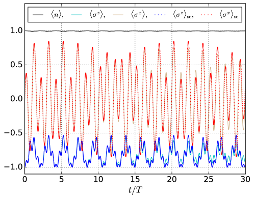
Figure 3: Emergent effective periodically driven dynamics in the semi-classical limit of the quantised light-atom interaction. The solid lines represent expectation values in the spin-photon basis, while dashed lines – the corresponding semi-classical quantities. The parameters are $A/\Delta=1$, $\Omega/\Delta=3.5$. The photon Hilbert space has a total number of $N_{\mathrm{ph,tot}}=60$ states, and the mean number of photons in the initial coherent state is $N_{\mathrm{ph}}=30$.

Figure 3 a shows a comparison between the quantum and the semi-classical time evolution of all observables $\mathcal{O}$ as defined above. As expected, we find a reasonable agreement with the deviation at longer times increasing, depending on the number of photons used, and the drive frequency.

Code Analysis—We used the following compact QuSpin code to produce these results. First we load the required classes, methods and functions to do the calculation:

Next, we define the model parameters as follows:

To set up the spin-photon Hamiltonian, we first build the site-coupling lists. The ph_energy list does not require the specification of a lattice site index, since the latter is not defined for the photon sector. The at_energy list, on the other hand, requires the input of the lattice site for the $\sigma^{z}$ operator: since we consider a single two-level system or, equivalently – a single-site chain, this index is 0. The spin-photon coupling lists absorb and emit also require the site index which refers to the corresponding Pauli matrices: in this model – 0 again due to dimensional constraints.

To build the static operator list, we use the | symbol in the operator string to distinguish the spin and photon operators: spin operators always come to the left of the |-symbol, while photon operators – to the right. For convenience, the identity operator I can be omitted, such that I|n is the same as |n, and z|I is equivalent to z|, respectively. The dynamic list is empty since the spin-photon Hamiltonian is time-independent.

To build the spin-photon basis, we call the function photon_basis and use spin_basis_1d as the first argument. We need to specify the number of spin lattice sites, and the total number of harmonic oscillator (a.k.a photon) states. Building the Hamiltonian works as in Sec. 2.2 and 2.3.

We now set up the time-periodic semi-classical Hamiltonian which is defined on the spin Hilbert space only; thus we use a spin_basis_1d basis object. We use the dynamic_sc list to define the time-dependence.

Next, we define the initial state as a product state, see Eq. (18). Notice that in the QuSpin spin_basis_1d basis convention the state $|\downarrow\;\rangle=(1,0)^{t}$. This is because the spin basis states are coded using their bit representations and the state of all spins pointing down is assigned the integer 0. To define the oscillator (a.k.a. photon) coherent state with mean photon number $N_{\mathrm{ph}}$, we use the function coherent_state: its first argument is the eigenvalue of the annihilation operator $a$, while the second argument is the total number of oscillator states.

The next step is to define a vector of stroboscopic times, using the class Floquet_t_vec. Unlike in Sec. 2.3, here we are also interested in the non-stroboscopic times in between the perfect periods $lT$. Thus, we omit the optional argument len_T making use of the default value set to len_T=100, meaning that there are now $100$ time points within each period.

We now time evolve the initial state both in the atom-photon, and the semi-classical cases using the hamiltonian class method evolve, as before. Once again, we define the solution psi_t as a generator expression using the optional argument iterate=True.

Last, we define the observables of interest, using the hamiltonian class with unit coupling constants. Since each observable represents a single operator, we refrain from defining operator lists and set up the observables in-line. Note that the main difference in defining the Pauli operators in the atom-photon and the semi-classical cases below (apart from the | notation), is the basis argument, defined in lines 62-63. The Python dictionaries obs_args and obs_args_sc represent another way of passing optional keyword arguments to the hamiltonian function. Here we also disable the automatic symmetry and hermiticity checks.

Finally, we calculate the time-dependent expectation values using the measurements tool function obs_vs_time. Its arguments are the time-dependent state psi_t, the vector of times t.vals, and a dictionary of all observables of interest, and were discussed in Sec. 2.3. obs_vs_time returns a dictionary with all time-dependent expectations stored under the same keys they were passed. They can be accessed as shown in lines 75 and 78, respectively.

The complete code including the lines that produce Fig. 3 is available in Example Code 4.

3 Future Perspectives for QuSpin

We have demonstrated that the QuSpin functionality allows the user to do many different kinds of ED calculations. In one spatial dimension, one also has the option of using a wide range of available symmetries. The reader might have noticed that, provided the study does not require the use of symmetries (e.g. a fully disordered 2D model), one can specify the site-coupling lists such as to build higher-dimensional Hamiltonians, using the spin_basis_1d class. Setting up higher-dimensional Hamiltonians with symmetries is possible in limited cases, too, when they can be uniquely mapped to one-dimensional systems.

In addition to the features we have discussed in this paper, there are many other functions defined inQuSpin which are all listed in the Documentation (Appendix D). Some of the more interesting ones include the tensor_basis class which constructs a new basis object out of two other basis objects, thus implementing the tensor product. This can be employed, e.g., to study interacting ladders with hard-core bosons. Another class which is useful for state-of-the-art calculations is the HamiltonianOperator class. It does the matrix vector product without actually storing the matrix elements which significantly reduces the amount of memory needed to do this operation. This is particularly suited for diagonalising very large spin chains using eigsh, as it only requires on the order of a hundred calls of the matrix vector product to solve for a few eigenvalues and eigenvectors (for a specific example, see the documentation in App. D). A recent addition to the tools module is the block_tools module. This module contains a class which projects an initial state in the full Hilbert space to a set of user provided symmetry sectors and then evolves each block in parallel (possibly over many CPU core’s) with a single function call. This is useful in cases where the intial state may not obey the given symmetries of the Hamiltonian used to evolve the state, for example when calculating non-equal time correlation functions. Finally the hamiltonian class is not just limited to matrices generated in our code from the operator strings. In general, this class also takes arbitrary matrices as inputs for both static and dynamic operators; therefore, one can use all of the packages functionality for any user-defined matrix.

We have set up the code to make it easily generalisable to different types of systems. We are currently working towards adding the one-dimensional symmetries for spinless and spinful fermions, but we are hoping to eventually add higher spins and bosons, too. Farther into the future we may implement a number of two dimensional lattices as well as their symmetries. We also welcome anyone who is interested in contributing to this project to reach out to the authors with any questions they may have about the package organisation. All modifications can be proposed through the pull request system on github.com.

We would much appreciate it if the users could report bugs using the issues forum in the QuSpin online repository.

Appendix A Installation Guide in a Few Steps

QuSpin is currently only being supported for Python 2.7 and Python 3.5 and so one must make sure to install this version of Python. We recommend the use of the free package manager Anaconda which installs Python and manages its packages. For a lighter installation, one can use miniconda.

A.1 Mac OS X/Linux

To install Anaconda/miniconda all one has to do is execute the installation script with administrative privilege. To do this, open up the terminal and go to the folder containing the downloaded installation file and execute the following command:

⬇

$ sudo bash <installation_file>

You will be prompted to enter your password. Follow the prompts of the installation. We recommend that you allow the installer to prepend the installation directory to your PATH variable which will make sure this installation of Python will be called when executing a Python script in the terminal. If this is not done then you will have to do this manually in your bash profile file:

⬇

$ export PATH="path_to/anaconda/bin:$PATH"

Installing via Anaconda.—Once you have Anaconda/miniconda installed, all you have to do to install QuSpin is to execute the following command into the terminal:

⬇

$ conda install -c weinbe58 quspin

If asked to install new packages just say ‘yes’. To keep the code up-to-date, just run this command regularly.

Installing Manually.—Installing the package manually is not recommended unless the above method failed. Note that you must have the Python packages NumPy, SciPy, and Joblib installed before installing QuSpin. Once all the prerequisite packages are installed, one can download the source code from github and then extract the code to whichever directory one desires. Open the terminal and go to the top level directory of the source code and execute:

⬇

$ python setup.py install --record install_file.txt

This will compile the source code and copy it to the installation directory of Python recording the installation location to install_file.txt. To update the code, you must first completely remove the current version installed and then install the new code. The install_file.txt can be used to remove the package by running:

⬇

$ cat install_file.txt | xargs rm -rf.

A.2 Windows

To install Anaconda/miniconda on Windows, download the installer and execute it to install the program. Once Anaconda/miniconda is installed open the conda terminal and do one of the following to install the package:

Installing via Anaconda.—Once you have Anaconda/miniconda installed all you have to do to install QuSpin is to execute the following command into the terminal:

⬇

> conda install -c weinbe58 quspin

If asked to install new packages just say ‘yes’. To update the code just run this command regularly.

Installing Manually.—Installing the package manually is not recommended unless the above method failed. Note that you must have NumPy, SciPy, and Joblib installed before installing QuSpin. Once all the prerequisite packages are installed, one can download the source code from github and then extract the code to whichever directory one desires. Open the terminal and go to the top level directory of the source code and then execute:

⬇

> python setup.py install --record install_file.txt

This will compile the source code and copy it to the installation directory of Python and record the installation location to install_file.txt. To update the code you must first completely remove the current version installed and then install the new code.

Appendix B Basic Use of Command Line to Run Python

In this appendix we will review how to use the command line for Windows and OS X/Linux to navigate your computer’s folders/directories and run the Python scripts.

B.1 Mac OS X/Linux

Some basic commands:

• change directory:

  ⬇

  $ cd < path_to_directory >

• list files in current directory:

  ⬇

  $ ls

  list files in another directory:

  ⬇

  $ ls < path_to_directory >

• make new directory:

  ⬇

  $ mkdir <path>/< directory_name >

• copy file:

  ⬇

  $ cp < path >/< file_name > < new_path >/< new_file_name >

• move file or change file name:

  ⬇

  $ mv < path >/< file_name > < new_path >/< new_file_name >

• remove file:

  ⬇

  $ rm < path_to_file >/< file_name >

Unix also has an auto complete feature if one hits the TAB key. It will complete a word or stop when it matches more than one file/folder name. The current directory is denoted by "." and the directory above is "..". Now, to execute a Python script all one has to do is open your terminal and navigate to the directory which contains the python script. To execute the script just use the following command:

⬇

$ python script.py

It’s that simple!

B.2 Windows

Some basic commands:

• change directory:

  ⬇

  > cd < path_to_directory >

• list files in current directory:

  ⬇

  > dir

  list files in another directory:

  ⬇

  > dir < path_to_directory >

• make new directory:

  ⬇

  > mkdir <path>\< directory_name >

• copy file:

  ⬇

  > copy < path >\< file_name > < new_path >\< new_file_name >

• move file or change file name:

  ⬇

  > move < path >\< file_name > < new_path >\< new_file_name >

• remove file:

  ⬇

  > erase < path >\< file_name >

Windows also has a auto complete feature using the TAB key but instead of stopping when there multiple files/folders with the same name, it will complete it with the first file alphabetically. The current directory is denoted by "." and the directory above is "..".

B.3 Execute Python Script (any operating system)

To execute a Python script all one has to do is open up a terminal and navigate to the directory which contains the Python script. Python can be recognised by the extension .py. To execute the script just use the following command:

⬇

python script.py

It’s that simple!

Appendix C Complete Example Codes

In this appendix, we give the complete python scripts for the four examples discussed in Sec. 2. In case the reader has trouble with the TAB spaces when copying from the code environments below, the scripts can be downloaded from github at: https://github.com/weinbe58/QuSpin/tree/master/examples

QuSpin Example Code 1: Exact Diagonalisation of the XXZ Model

QuSpin Example Code 2: Adiabatic Control of Parameters in MBL Phases

QuSpin Example Code 3: Heating in Periodically Driven Spin Chains

QuSpin Example Code 4: Quantised Light-Atom Interactions in the Semi-classical Limit

Appendix D Package Documentation

In QuSpin quantum many-body operators are represented as matrices. The computation of these matrices are done through custom code written in Cython. Cython is an optimizing static compiler which takes code written in a syntax similar to Python, and compiles it into a highly efficient C/C++ shared library. These libraries are then easily interfaced with Python, but can run orders of magnitude faster than pure Python code [53]. The matrices are stored in a sparse matrix format using the sparse matrix library of SciPy [24]. This allows QuSpin to easily interface with mature Python packages, such as NumPy, SciPy, any many others. These packages provide reliable state-of-the-art tools for scientific computation as well as support from the Python community to regularly improve and update them [54, 55, 56, 24]. Moreover, we have included specific functionality in QuSpin which uses NumPy and SciPy to do many desired calculations common to ED studies, while making sure the user only has to call a few NumPy or SciPy functions directly. The complete up-to-date documentation for the package is available online under:

https://github.com/weinbe58/QuSpin/#quspin

References

- [1] L. Pollet, Recent developments in quantum monte carlo simulations with applications for cold gases, Reports on Progress in Physics 75(9), 094501 (2012).
- [2] W. M. C. Foulkes, L. Mitas, R. J. Needs and G. Rajagopal, Quantum monte carlo simulations of solids, Rev. Mod. Phys. 73, 33 (2001), 10.1103/RevModPhys.73.33.
- [3] P. H. Acioli, Review of quantum monte carlo methods and their applications, Journal of Molecular Structure: THEOCHEM 394(2), 75 (1997), http://dx.doi.org/10.1016/S0166-1280(96)04821-X.
- [4] A. J. Daley, C. Kollath, U. Schollwöck and G. Vidal, Time-dependent density-matrix renormalization-group using adaptive effective hilbert spaces, Journal of Statistical Mechanics: Theory and Experiment 2004(04), P04005 (2004).
- [5] U. Schollwöck, The density-matrix renormalization group, Rev. Mod. Phys. 77, 259 (2005), 10.1103/RevModPhys.77.259.
- [6] U. Schollwöck, The density-matrix renormalization group in the age of matrix product states, Annals of Physics 326(1), 96 (2011), http://dx.doi.org/10.1016/j.aop.2010.09.012, January 2011 Special Issue.
- [7] A. Georges, G. Kotliar, W. Krauth and M. J. Rozenberg, Dynamical mean-field theory of strongly correlated fermion systems and the limit of infinite dimensions, Rev. Mod. Phys. 68, 13 (1996), 10.1103/RevModPhys.68.13.
- [8] G. Kotliar, S. Y. Savrasov, K. Haule, V. S. Oudovenko, O. Parcollet and C. A. Marianetti, Electronic structure calculations with dynamical mean-field theory, Rev. Mod. Phys. 78, 865 (2006), 10.1103/RevModPhys.78.865.
- [9] H. Aoki, N. Tsuji, M. Eckstein, M. Kollar, T. Oka and P. Werner, Nonequilibrium dynamical mean-field theory and its applications, Rev. Mod. Phys. 86, 779 (2014), 10.1103/RevModPhys.86.779.
- [10] F. Alet, P. Dayal, A. Grzesik, A. Honecker, M. Körner, A. Läuchli, S. R. Manmana, I. P. McCulloch, F. Michel, R. M. Noack, G. Schmid, U. Schollwöck et al., The alps project: Open source software for strongly correlated systems, Journal of the Physical Society of Japan 74(Suppl), 30 (2005), 10.1143/JPSJS.74S.30, http://dx.doi.org/10.1143/JPSJS.74S.30.
- [11] A. Albuquerque, F. Alet, P. Corboz, P. Dayal, A. Feiguin, S. Fuchs, L. Gamper, E. Gull, S. Gürtler, A. Honecker, R. Igarashi, M. Körner et al., The {ALPS} project release 1.3: Open-source software for strongly correlated systems, Journal of Magnetism and Magnetic Materials 310(2, Part 2), 1187 (2007), http://dx.doi.org/10.1016/j.jmmm.2006.10.304, Proceedings of the 17th International Conference on MagnetismThe International Conference on Magnetism.
- [12] B. Bauer, L. D. Carr, H. G. Evertz, A. Feiguin, J. Freire, S. Fuchs, L. Gamper, J. Gukelberger, E. Gull, S. Guertler, A. Hehn, R. Igarashi et al., The alps project release 2.0: open source software for strongly correlated systems, Journal of Statistical Mechanics: Theory and Experiment 2011(05), P05001 (2011).
- [13] M. Dolfi, B. Bauer, S. Keller, A. Kosenkov, T. Ewart, A. Kantian, T. Giamarchi and M. Troyer, Matrix product state applications for the {ALPS} project, Computer Physics Communications 185(12), 3430 (2014), http://dx.doi.org/10.1016/j.cpc.2014.08.019.
- [14] E. M. Stoudenmire, S. R. White et al., ITensor: C++ library for implementing tensor product wavefunction calculations (2011–).
- [15] D. J. S. Al-Assam, S. R. Clark and TNT Development team, Tensor network theory library, beta version 1.2.0 (2016–).
- [16] J. Johansson, P. Nation and F. Nori, Qutip: An open-source python framework for the dynamics of open quantum systems, Computer Physics Communications 183(8), 1760 (2012), http://dx.doi.org/10.1016/j.cpc.2012.02.021.
- [17] J. Johansson, P. Nation and F. Nori, Qutip 2: A python framework for the dynamics of open quantum systems, Computer Physics Communications 184(4), 1234 (2013), http://dx.doi.org/10.1016/j.cpc.2012.11.019.
- [18] J. G. Wright and B. S. Shastry, Diracq: A quantum many-body physics package, arXiv preprint arXiv:1301.4494 (2013).
- [19] J. R. Schrieffer and P. A. Wolff, Relation between the anderson and kondo hamiltonians, Phys. Rev. 149, 491 (1966), 10.1103/PhysRev.149.491.
- [20] S. Bravyi, D. P. DiVincenzo and D. Loss, Schrieffer–wolff transformation for quantum many-body systems, Annals of Physics 326(10), 2793 (2011), http://dx.doi.org/10.1016/j.aop.2011.06.004.
- [21] M. Bukov, M. Kolodrubetz and A. Polkovnikov, Schrieffer-wolff transformation for periodically driven systems: Strongly correlated systems with artificial gauge fields, Phys. Rev. Lett. 116, 125301 (2016), 10.1103/PhysRevLett.116.125301.
- [22] N. Goldman and J. Dalibard, Periodically driven quantum systems: Effective hamiltonians and engineered gauge fields, Phys. Rev. X 4, 031027 (2014), 10.1103/PhysRevX.4.031027.
- [23] M. Bukov, L. D’Alessio and A. Polkovnikov, Universal high-frequency behavior of periodically driven systems: from dynamical stabilization to floquet engineering, Advances in Physics 64(2), 139 (2015), 10.1080/00018732.2015.1055918, http://dx.doi.org/10.1080/00018732.2015.1055918.
- [24] E. Jones, T. Oliphant, P. Peterson et al., SciPy: Open source scientific tools for Python (2001–).
- [25] D. Basko, I. Aleiner and B. Altshuler, Metal–insulator transition in a weakly interacting many-electron system with localized single-particle states, Annals of Physics 321(5), 1126 (2006), http://dx.doi.org/10.1016/j.aop.2005.11.014.
- [26] I. V. Gornyi, A. D. Mirlin and D. G. Polyakov, Interacting electrons in disordered wires: Anderson localization and low- transport, Phys. Rev. Lett. 95, 206603 (2005), 10.1103/PhysRevLett.95.206603.
- [27] J. Z. Imbrie, On many-body localization for quantum spin chains, Journal of Statistical Physics 163(5), 998 (2016), 10.1007/s10955-016-1508-x.
- [28] V. Oganesyan and D. A. Huse, Localization of interacting fermions at high temperature, Phys. Rev. B 75, 155111 (2007), 10.1103/PhysRevB.75.155111.
- [29] A. Pal and D. A. Huse, Many-body localization phase transition, Phys. Rev. B 82, 174411 (2010), 10.1103/PhysRevB.82.174411.
- [30] R. Vosk and E. Altman, Many-body localization in one dimension as a dynamical renormalization group fixed point, Phys. Rev. Lett. 110, 067204 (2013), 10.1103/PhysRevLett.110.067204.
- [31] R. Nandkishore and D. A. Huse, Many-body localization and thermalization in quantum statistical mechanics, Annual Review of Condensed Matter Physics 6(1), 15 (2015), 10.1146/annurev-conmatphys-031214-014726, http://dx.doi.org/10.1146/annurev-conmatphys-031214-014726.
- [32] V. Khemani, R. Nandkishore and S. L. Sondhi, Nonlocal adiabatic response of a localized system to local manipulations, Nature Physics 11, 560 (2015), 10.1038/nphys3344.
- [33] M. Schreiber, S. S. Hodgman, P. Bordia, H. P. Lüschen, M. H. Fischer, R. Vosk, E. Altman, U. Schneider and I. Bloch, Observation of many-body localization of interacting fermions in a quasirandom optical lattice, Science 349(6250), 842 (2015), 10.1126/science.aaa7432, http://science.sciencemag.org/content/349/6250/842.full.pdf.
- [34] M. Ovadia, D. Kalok, I. Tamir, S. Mitra, B. Sacépé and D. Shahar, Evidence for a finite-temperature insulator, Scientific Reports 5, 13503 (2015), 10.1038/srep13503.
- [35] P. Bordia, H. P. Lüschen, S. S. Hodgman, M. Schreiber, I. Bloch and U. Schneider, Coupling identical one-dimensional many-body localized systems, Phys. Rev. Lett. 116, 140401 (2016), 10.1103/PhysRevLett.116.140401.
- [36] J. Smith, A. Lee, P. Richerme, B. Neyenhuis, P. W. Hess, P. Hauke, M. Heyl, D. A. Huse and C. Monroe, Many-body localization in a quantum simulator with programmable random disorder, Nature Physics 12, 907–911 (2016), 10.1038/nphys3783.
- [37] J.-y. Choi, S. Hild, J. Zeiher, P. Schauß, A. Rubio-Abadal, T. Yefsah, V. Khemani, D. A. Huse, I. Bloch and C. Gross, Exploring the many-body localization transition in two dimensions, Science 352(6293), 1547 (2016), 10.1126/science.aaf8834, http://science.sciencemag.org/content/352/6293/1547.full.pdf.
- [38] P. Weinberg, M. Bukov, L. D’Alessio, A. Polkovnikov, S. Vajna and M. Kolodrubetz, Adiabatic perturbation theory and geometry of periodically-driven systems, arXiv preprint arXiv:1606.02229 (2016).
- [39] D. J. Luitz, N. Laflorencie and F. Alet, Many-body localization edge in the random-field heisenberg chain, Phys. Rev. B 91, 081103 (2015), 10.1103/PhysRevB.91.081103.
- [40] L. Zhang, H. Kim and D. A. Huse, Thermalization of entanglement, Phys. Rev. E 91, 062128 (2015), 10.1103/PhysRevE.91.062128.
- [41] T. Prosen, Time evolution of a quantum many-body system: Transition from integrability to ergodicity in the thermodynamic limit, Phys. Rev. Lett. 80, 1808 (1998), 10.1103/PhysRevLett.80.1808.
- [42] T. Prosen, Ergodic properties of a generic nonintegrable quantum many-body system in the thermodynamic limit, Phys. Rev. E 60, 3949 (1999), 10.1103/PhysRevE.60.3949.
- [43] M. Bukov, L. D’Alessio and A. Polkovnikov, Universal high-frequency behavior of periodically driven systems: from dynamical stabilization to floquet engineering, Advances in Physics 64(2), 139 (2015), 10.1080/00018732.2015.1055918, http://dx.doi.org/10.1080/00018732.2015.1055918.
- [44] M. Bukov, Floquet Engineering in Closed Periodically Driven Quantum Systems: From Dynamical Localisation to Ultracold Topological Matter, Ph.D. thesis, Boston University (2016).
- [45] M. Bukov, M. Heyl, D. A. Huse and A. Polkovnikov, Heating and many-body resonances in a periodically driven two-band system, Phys. Rev. B 93, 155132 (2016), 10.1103/PhysRevB.93.155132.
- [46] D. A. Abanin, W. De Roeck and F. m. c. Huveneers, Exponentially slow heating in periodically driven many-body systems, Phys. Rev. Lett. 115, 256803 (2015), 10.1103/PhysRevLett.115.256803.
- [47] T. Kuwahara, T. Mori and K. Saito, Floquet–magnus theory and generic transient dynamics in periodically driven many-body quantum systems, Annals of Physics 367, 96 (2016), http://dx.doi.org/10.1016/j.aop.2016.01.012.
- [48] T. Mori, T. Kuwahara and K. Saito, Rigorous bound on energy absorption and generic relaxation in periodically driven quantum systems, Phys. Rev. Lett. 116, 120401 (2016), 10.1103/PhysRevLett.116.120401.
- [49] D. Abanin, W. De Roeck and W. W. Ho, Effective hamiltonians, prethermalization and slow energy absorption in periodically driven many-body systems, arXiv preprint arXiv:1510.03405 p. 1510.03405 (2015).
- [50] L. D’Alessio, Y. Kafri, A. Polkovnikov and M. Rigol, From quantum chaos and eigenstate thermalization to statistical mechanics and thermodynamics, Advances in Physics 65, 239 (2016), 10.1080/00018732.2016.1198134, http://dx.doi.org/10.1080/00018732.2016.1198134.
- [51] A. W. Sandvik, Computational studies of quantum spin systems, AIP Conference Proceedings 1297(1), 135 (2010), http://dx.doi.org/10.1063/1.3518900.
- [52] S. Haroche and J. Raimond, Exploring the Quantum: Atoms, Cavities, and Photons, Oxford Graduate Texts. OUP Oxford, ISBN 9780198509141 (2006).
- [53] S. Behnel, R. Bradshaw, C. Citro, L. Dalcin, D. S. Seljebotn and K. Smith, Cython: The best of both worlds, Computing in Science & Engineering 13(2), 31 (2011), http://dx.doi.org/10.1109/MCSE.2010.118.
- [54] S. v. d. Walt, S. C. Colbert and G. Varoquaux, The numpy array: A structure for efficient numerical computation, Computing in Science & Engineering 13(2), 22 (2011), http://dx.doi.org/10.1109/MCSE.2011.37.
- [55] T. E. Oliphant, Python for scientific computing, Computing in Science & Engineering 9(3), 10 (2007), http://dx.doi.org/10.1109/MCSE.2007.58.
- [56] K. J. Millman and M. Aivazis, Python for scientists and engineers, Computing in Science & Engineering 13(2), 9 (2011), http://dx.doi.org/10.1109/MCSE.2011.36.