Solitons of a vector model on the honeycomb lattice.

Abstract

We study a simple nonlinear vector model defined on the honeycomb lattice. We propose a bilinearization scheme for the field equations and demonstrate that the resulting system is closely related to the well-studied integrable models, such as the Hirota bilinear difference equation and the Ablowitz-Ladik system. This result is used to derive the $N$-soliton solutions.

1 Introduction.

We study a simple nonlinear model defined on the honeycomb lattice (HL). The main aim of this work is to apply the direct methods of the soliton theory to the case of the ‘non-square’, i.e. different from $\mathbb{Z}^{2}$, two-dimensional lattices.

There has been considerable interest in the integrable nonlinear models on such lattices, and even arbitrary graphs (see, for example, [1, 2, 3, 4, 5, 6, 7, 8]). The results of these studies provide answers to many questions arising in the theory of integrable systems. However, if we consider the problem of finding solutions, there is still, in our opinion, much to be done in this field. The case is that many of the standard tools have not been adapted so far to the non-square lattices. For example, for many models on graphs (in particular, as is shown in [3], for all models that possess the property of the three-dimensional consistency [9]) one can construct a special form of the Lax (or zero-curvature) representation, called the “trivial monodromy representation” in [2], which has been successively used as an integrability test. Nevertheless, the graph analogue of the inverse scattering transform (IST), that is based on this representation, has not been elaborated yet. In this situation, the main tool to derive explicit solutions are the so-called direct methods, for which the lack of natural ways to separate variables (as in the case of HL) seems to be less important than for the IST-like approaches. Of course, to make these methods suitable for the HL, one has to modify the standard procedure. However, as a reader will see, this can be done by rather elementary means.

In this work we present the explicit $N$-soliton solutions for the vector model which is described in section 2. In section 3, we bilinearize the field equations and convert them into a simple system of three-point equations. In section 4, we discuss this system, and show that it is closely related to the well-studied integrable models, such as the Hirota bilinear difference and the Ablowitz-Ladik equations. Then, using the already known results as well as the ones derived in section 4, we present, in section 5, the $N$-soliton solutions for the field equations of our model.

2 The model and the main equations.

The model which we study in this paper describes the three-dimensional vectors (fields) $\boldsymbol{\phi}=\boldsymbol{\phi}(\mathsf{v})\in\mathbb{R}^{3}$ defined at the vertices $\mathsf{v}$ of the HL with the logarithmic interaction between the nearest neighbours,

$$\mathcal{S}=\sum\limits_{\mathsf{v^{\prime}}\sim\mathsf{v^{\prime\prime}}}\Gamma_{(\mathsf{v^{\prime}},\mathsf{v^{\prime\prime}})}\;\ln\left[1+\left(\boldsymbol{\phi}(\mathsf{v^{\prime}}),\boldsymbol{\phi}(\mathsf{v^{\prime\prime}})\right)\right]$$ (2.1)

where the notation $\mathsf{v^{\prime}}\sim\mathsf{v^{\prime\prime}}$ means that the vertices $\mathsf{v^{\prime}}$ and $\mathsf{v^{\prime\prime}}$ are connected by an edge of the HL, $\left(\boldsymbol{\phi}^{\prime},\boldsymbol{\phi}^{\prime\prime}\right)$ is the standard scalar product in $\mathbb{R}^{3}$ and $\Gamma_{(\mathsf{v^{\prime}},\mathsf{v^{\prime\prime}})}$ are constants which take the values $\Gamma_{1}$, $\Gamma_{2}$ or $\Gamma_{3}$ depending on the direction of the edge $(\mathsf{v^{\prime}},\mathsf{v^{\prime\prime}})$ connecting nodes $\mathsf{v^{\prime}}$ and $\mathsf{v^{\prime\prime}}$ (see figure 1) and satisfy the following restriction:

$$\sum_{\mathsf{v}^{\prime}}\Gamma_{(\mathsf{v},\mathsf{v^{\prime}})}=0\quad\mbox{for all}\;\mathsf{v}$$ (2.2)

with the summation over all nodes adjacent to $\mathsf{v}$.

The logarithmic interaction in (2.1) between the vectors $\boldsymbol{\phi}$ is not new to the theory of integrable systems (see, for example, [10, 11, 12]) and can be viewed as the classical$+$integrable analogue of the famous Heisenberg interaction of the quantum mechanics. In this sense, the model considered here is closely related to the one-dimensional Ishimori spin chain [10]. However, there is an essential difference: we do not impose restrictions like $\boldsymbol{\phi}^{2}=1$ which are crucial for models describing the spin-like systems.

On the other hand, this model can be considered as a vector generalization of one of the ‘universal’ integrable models of the paper [2] which was studied in [3, 13].

Considering the condition (2.2), it should be noted that restrictions of this type often appear in the studies of integrable models. If we, for example, look at the Hirota bilinear difference equation (HBDE), the restriction similar to (2.1) is present in the most of the works devoted to this system (including the original paper [14]). However, as it has been demonstrated in, for example, [15], it is not needed for the integrability (it is a widespread opinion that it is required for the existence of the Hirota-form soliton solutions).

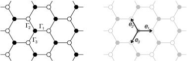
Figure 1: Bipartition of the HL, interaction constants and base vectors. The vertices that belong to $\Lambda^{+}$ are shown by black circles and the vertices that belong to $\Lambda^{-}$ are shown by white ones.

Hereafter, we use the vector notation. We introduce coplanar vectors $\boldsymbol{e}_{1}$, $\boldsymbol{e}_{2}$ and $\boldsymbol{e}_{3}$, that generate the HL and are related by

$$\sum_{i=1}^{3}\boldsymbol{e}_{i}=\boldsymbol{0},$$ (2.3)

the set $\Lambda$ of the lattice vectors $\boldsymbol{n}$ (positions of the vertices of the HL),

$$\Lambda=\left\{\left.\boldsymbol{n}=\sum_{i=1}^{3}n_{i}\boldsymbol{e}_{i},\quad n_{i}\in\mathbb{Z}\quad\right|\quad\sum_{i=1}^{3}n_{i}\neq 2\mathop{\mbox{mod}}3\right\},$$ (2.4)

which can be decomposed as

$$\Lambda=\Lambda^{+}\cup\Lambda^{-}$$ (2.5)

with

$$\begin{array}[]{l}\Lambda^{+}=\left\{\left.\boldsymbol{n}=\sum\limits_{i=1}^{3}n_{i}\boldsymbol{e}_{i},\quad n_{i}\in\mathbb{Z}\quad\right|\quad\sum\limits_{i=1}^{3}n_{i}=0\mathop{\mbox{mod}}3\;\right\},\\[11.38109pt] \Lambda^{-}=\left\{\left.\boldsymbol{n}=\sum\limits_{i=1}^{3}n_{i}\boldsymbol{e}_{i},\quad n_{i}\in\mathbb{Z}\quad\right|\quad\sum\limits_{i=1}^{3}n_{i}=1\mathop{\mbox{mod}}3\;\right\}\end{array}$$ (2.6)

(this is a manifestation of the fact that the HL is a bipartite graph) and write $\boldsymbol{\phi}(\boldsymbol{n})$ instead of $\boldsymbol{\phi}(\mathsf{v})$.

In the $\boldsymbol{n}$-terms the action (2.1) can be presented as

$$\mathcal{S} = \sum\limits_{\boldsymbol{n}\in\Lambda^{+}}\sum\limits_{i=1}^{3}\Gamma_{i}\ln\left[1+\left(\boldsymbol{\phi}(\boldsymbol{n}),\boldsymbol{\phi}(\boldsymbol{n}+\boldsymbol{e}_{i})\right)\right]$$ (2.0a)

$$= \sum\limits_{\boldsymbol{n}\in\Lambda^{-}}\sum\limits_{i=1}^{3}\Gamma_{i}\ln\left[1+\left(\boldsymbol{\phi}(\boldsymbol{n}),\boldsymbol{\phi}(\boldsymbol{n}-\boldsymbol{e}_{i})\right)\right]$$ (2.0b)

where we use, instead of $\Gamma_{(\mathsf{v^{\prime}},\mathsf{v^{\prime\prime}})}$, constants $\Gamma_{i}$ ($i=1,2,3$), $\Gamma_{(\mathsf{v^{\prime}},\mathsf{v^{\prime\prime}})}=\Gamma_{i}$ if the edge $(\mathsf{v^{\prime}},\mathsf{v^{\prime\prime}})$ is parallel to the vector $\boldsymbol{e}_{i}$ (see figure 1), subjected to the restriction (2.2),

$$\sum\limits_{i=1}^{3}\Gamma_{i}=0.$$ (2.1)

The ‘variational’ equations

$$\left.\partial\mathcal{S}\right/\partial\boldsymbol{\phi}(\boldsymbol{n})=0,\qquad\boldsymbol{n}\in\Lambda$$ (2.2)

can be written as

$$\sum\limits_{i=1}^{3}\frac{\Gamma_{i}}{1+\left(\boldsymbol{\phi}(\boldsymbol{n}),\boldsymbol{\phi}(\boldsymbol{n}+\boldsymbol{e}_{i})\right)}\;\boldsymbol{\phi}(\boldsymbol{n}+\boldsymbol{e}_{i})=\boldsymbol{0} (\boldsymbol{n}\in\Lambda^{+})$$ (2.0a)

$$\sum\limits_{i=1}^{3}\frac{\Gamma_{i}}{1+\left(\boldsymbol{\phi}(\boldsymbol{n}),\boldsymbol{\phi}(\boldsymbol{n}-\boldsymbol{e}_{i})\right)}\;\boldsymbol{\phi}(\boldsymbol{n}-\boldsymbol{e}_{i})=\boldsymbol{0} (\boldsymbol{n}\in\Lambda^{-})$$ (2.0b)

Namely these equations are the main object of our study.

3 Solving the field equations.

In this section we reduce the field equations (2.2) to an already known bilinear system. The procedure, which is, for the most part, rather standard has a few non-trivial moments that stem from the structure of the HL.

3.1 Resolving the restriction (2.3).

To resolve the restriction (2.3) we, first, ‘replace’ the vectors $\boldsymbol{e}_{i}$ which obey (2.3) with new arbitrary vectors $\boldsymbol{\alpha}_{i}$ ($i=1,2,3$) from some auxiliary space $\mathbb{V}$. This means that we consider instead of functions of $\boldsymbol{n}=\sum_{i=1}^{3}n_{i}\boldsymbol{e}_{i}$, functions of $\sum_{i=1}^{3}n_{i}\left(\boldsymbol{\alpha}_{i}-\boldsymbol{\delta}\right)$ with $\boldsymbol{\delta}=\frac{1}{3}\sum_{i=1}^{3}\boldsymbol{\alpha}_{i}.$ Thus, we introduce the map $\boldsymbol{x}:\Lambda\to\mathbb{V}$,

$$\boldsymbol{n}=\sum_{i=1}^{3}n_{i}\boldsymbol{e}_{i}\quad\to\quad\boldsymbol{x}(\boldsymbol{n})=\sum_{i=1}^{3}n_{i}\left(\boldsymbol{\alpha}_{i}-\boldsymbol{\delta}\right),\quad\boldsymbol{\delta}=\frac{1}{3}\sum_{i=1}^{3}\boldsymbol{\alpha}_{i}$$ (3.1)

whose image belongs to the two-dimensional plane from our auxiliary space $\mathbb{V}$. The advantage of the $\boldsymbol{x}$-representation is that it automatically (for arbitrary $\boldsymbol{\alpha}_{i}$) takes into account the restriction (2.3), $\boldsymbol{x}\left(\boldsymbol{n}+\sum_{i=1}^{3}\boldsymbol{e}_{i}\right)=\boldsymbol{x}(\boldsymbol{n})$.

Secondly, in order to simplify the following equations and eliminate the explicit appearance of $\boldsymbol{\delta}$, we introduce, instead of the vectors $\boldsymbol{\phi}$, new vectors, $\boldsymbol{\phi}_{+}$ and $\boldsymbol{\phi}_{-}$,

$$\boldsymbol{\phi}(\boldsymbol{n})=\left\{\begin{array}[]{rcl}\boldsymbol{\phi}_{+}(\boldsymbol{x}(\boldsymbol{n})+\boldsymbol{\delta})&&(\boldsymbol{n}\in\Lambda^{+})\\ \boldsymbol{\phi}_{-}(\boldsymbol{x}(\boldsymbol{n})-\boldsymbol{\delta})&&(\boldsymbol{n}\in\Lambda^{-}).\end{array}\right.$$ (3.2)

In new terms, we can rewrite the equations we want to solve as

$$\;\sum\limits_{i=1}^{3}\frac{\Gamma_{i}}{1+\left(\boldsymbol{\phi}_{+}(\boldsymbol{x}_{+}),\boldsymbol{\phi}_{-}(\boldsymbol{x}_{+}-\boldsymbol{\alpha}_{i-1}-\boldsymbol{\alpha}_{i+1})\right)}\;\boldsymbol{\phi}_{-}(\boldsymbol{x}_{+}-\boldsymbol{\alpha}_{i-1}-\boldsymbol{\alpha}_{i+1})=\boldsymbol{0} (\boldsymbol{n}\in\Lambda^{+})$$ (3.0a)

$$\;\sum\limits_{i=1}^{3}\frac{\Gamma_{i}}{1+\left(\boldsymbol{\phi}_{+}(\boldsymbol{x}_{-}+\boldsymbol{\alpha}_{i-1}+\boldsymbol{\alpha}_{i+1}),\boldsymbol{\phi}_{-}(\boldsymbol{x}_{-})\right)}\;\boldsymbol{\phi}_{+}(\boldsymbol{x}_{-}+\boldsymbol{\alpha}_{i-1}+\boldsymbol{\alpha}_{i+1})=\boldsymbol{0} (\boldsymbol{n}\in\Lambda^{-})$$ (3.0b)

where $\boldsymbol{x}_{\pm}=\boldsymbol{x}(\boldsymbol{n})\pm\boldsymbol{\delta}$. In these equations, as well as in the rest of the paper, we use the following convention: all arithmetic operations with $\boldsymbol{\alpha}$- and $\Gamma$-indices are understood modulo $3$,

$$\boldsymbol{\alpha}_{i\pm 3}=\boldsymbol{\alpha}_{i},\qquad\Gamma_{i\pm 3}=\Gamma_{i}\qquad(i=1,2,3).$$ (3.1)

Looking at (3.2) one can see that the ‘natural’ domains of definition of the functions $\boldsymbol{\phi}_{+}$ and $\boldsymbol{\phi}_{-}$ are points of the lattices $\boldsymbol{x}(\Lambda^{\pm})\pm\boldsymbol{\delta}$ (which belong to parallel, but different, 2-planes of $\mathbb{V}$). However, we consider both $\boldsymbol{\phi}_{+}$ and $\boldsymbol{\phi}_{-}$ as defined on the whole $\mathbb{V}$ ($\boldsymbol{\phi}_{+},\boldsymbol{\phi}_{-}:\mathbb{V}\to\mathbb{R}^{3}$) and define them as solutions of the system similar to (3.2) but thought of as a system on $\mathbb{V}$:

$$\left\{\begin{array}[]{l}\sum\limits_{i=1}^{3}\Gamma_{i}\,H_{i}^{+}(\boldsymbol{x})\;\boldsymbol{\phi}_{-}(\boldsymbol{x}-\boldsymbol{\alpha}_{i-1}-\boldsymbol{\alpha}_{i+1})=\boldsymbol{0}\\ \sum\limits_{i=1}^{3}\Gamma_{i}\,H_{i}^{-}(\boldsymbol{x})\;\boldsymbol{\phi}_{+}(\boldsymbol{x}+\boldsymbol{\alpha}_{i-1}+\boldsymbol{\alpha}_{i+1})=\boldsymbol{0}\end{array}\right.\qquad(\boldsymbol{x}\in\mathbb{V})$$ (3.2)

where

$$H_{i}^{+}(\boldsymbol{x}) = \left[1+\left(\boldsymbol{\phi}_{+}(\boldsymbol{x}),\boldsymbol{\phi}_{-}(\boldsymbol{x}-\boldsymbol{\alpha}_{i-1}-\boldsymbol{\alpha}_{i+1})\right)\right]^{-1},$$ (3.0a)

$$H_{i}^{-}(\boldsymbol{x}) = \left[1+\left(\boldsymbol{\phi}_{+}(\boldsymbol{x}+\boldsymbol{\alpha}_{i-1}+\boldsymbol{\alpha}_{i+1}),\boldsymbol{\phi}_{-}(\boldsymbol{x})\right)\right]^{-1}.$$ (3.0b)

3.2 Ansatz.

The key step of our construction is the following ansatz:

$$\begin{array}[]{lcl}\boldsymbol{\phi}_{+}(\boldsymbol{x}+\boldsymbol{\alpha}_{j}+\boldsymbol{\alpha}_{k})&\propto&\boldsymbol{\phi}_{+}(\boldsymbol{x}+\boldsymbol{\alpha}_{j})-\boldsymbol{\phi}_{+}(\boldsymbol{x}+\boldsymbol{\alpha}_{k}),\\ \boldsymbol{\phi}_{-}(\boldsymbol{x}-\boldsymbol{\alpha}_{j}-\boldsymbol{\alpha}_{k})&\propto&\boldsymbol{\phi}_{-}(\boldsymbol{x}-\boldsymbol{\alpha}_{j})-\boldsymbol{\phi}_{-}(\boldsymbol{x}-\boldsymbol{\alpha}_{k}).\end{array}$$ (3.1)

Of course, this ansatz is rather restrictive. However, it leads to a rather wide range of solutions, which include the $N$-soliton solutions (as well as the so-called finite-gap, Toeplitz and other solutions).

In more detail, we require

$$\qquad H_{i}^{+}(\boldsymbol{x})\;\boldsymbol{\phi}_{-}(\boldsymbol{x}-\boldsymbol{\alpha}_{i-1}-\boldsymbol{\alpha}_{i+1}) = \frac{\boldsymbol{\phi}_{-}(\boldsymbol{x}-\boldsymbol{\alpha}_{i-1})-\boldsymbol{\phi}_{-}(\boldsymbol{x}-\boldsymbol{\alpha}_{i+1})}{\chi_{i-1}-\chi_{i+1}},$$ (3.0a)

$$\qquad H_{i}^{-}(\boldsymbol{x})\;\boldsymbol{\phi}_{+}(\boldsymbol{x}+\boldsymbol{\alpha}_{i-1}+\boldsymbol{\alpha}_{i+1}) = \frac{\boldsymbol{\phi}_{+}(\boldsymbol{x}+\boldsymbol{\alpha}_{i-1})-\boldsymbol{\phi}_{+}(\boldsymbol{x}+\boldsymbol{\alpha}_{i+1})}{\chi_{i-1}-\chi_{i+1}}$$ (3.0b)

with constants $\chi_{i}$ ($i=1,2,3$) which will be specified below. Again, we presume that $\chi_{i\pm 3}=\chi_{i}$.

With (3.2), equations (3.2) become

$$\sum\limits_{i=1}^{3}\hat{\Gamma}_{i}\,\boldsymbol{\phi}_{-}(\boldsymbol{x}-\boldsymbol{\alpha}_{i})=\boldsymbol{0},$$ (3.0a)

$$\sum\limits_{i=1}^{3}\hat{\Gamma}_{i}\,\boldsymbol{\phi}_{+}(\boldsymbol{x}+\boldsymbol{\alpha}_{i})=\boldsymbol{0}$$ (3.0b)

with constant $\hat{\Gamma}_{i}$,

$$\hat{\Gamma}_{i}=\frac{\Gamma_{i+1}}{\chi_{i}-\chi_{i-1}}+\frac{\Gamma_{i-1}}{\chi_{i}-\chi_{i+1}}.$$ (3.1)

It is easily seen that we can satisfy all equations (3.2) without imposing additional conditions upon the vectors $\boldsymbol{\phi}_{+}$ and $\boldsymbol{\phi}_{-}$ by making all $\hat{\Gamma}_{i}$ equal to zero. Solution of this elementary problem leads to the following restriction upon the constants $\chi_{i}$ that can be used in the ansatz (3.2):

$$\sum_{i=1}^{3}\Gamma_{i}\,\chi_{i}=0$$ (3.2)

(it is straightforward to verify that (3.2) indeed leads to $\hat{\Gamma}_{i}=0$). Thus, we have reduced our problem to equations (3.2), (3.2) together with (3.2).

3.3 Bilinerization.

Noting that $H_{i}^{\pm}$, considered as functions on $\mathbb{V}$, are related by simple shifts and using only one of them,

$$H_{i}(\boldsymbol{x}):=H_{i}^{-}(\boldsymbol{x}),\quad H_{i}^{+}(\boldsymbol{x})=H_{i}(\boldsymbol{x}-\boldsymbol{\alpha}_{i-1}-\boldsymbol{\alpha}_{i+1})$$ (3.3)

one arrives at the system

$$\quad\left(\chi_{i-1}-\chi_{i+1}\right)H_{i}(\boldsymbol{x})\;\boldsymbol{\phi}_{+}(\boldsymbol{x}+\boldsymbol{\alpha}_{i-1}+\boldsymbol{\alpha}_{i+1}) = \boldsymbol{\phi}_{+}(\boldsymbol{x}+\boldsymbol{\alpha}_{i-1})-\boldsymbol{\phi}_{+}(\boldsymbol{x}+\boldsymbol{\alpha}_{i+1}),$$ (3.0a)

$$\quad\left(\chi_{i-1}-\chi_{i+1}\right)H_{i}(\boldsymbol{x})\;\boldsymbol{\phi}_{-}(\boldsymbol{x}) = \boldsymbol{\phi}_{-}(\boldsymbol{x}+\boldsymbol{\alpha}_{i+1})-\boldsymbol{\phi}_{-}(\boldsymbol{x}+\boldsymbol{\alpha}_{i-1})$$ (3.0b)

and

$$\qquad H_{i}(\boldsymbol{x})=\left[1+\left(\boldsymbol{\phi}_{+}(\boldsymbol{x}+\boldsymbol{\alpha}_{i-1}+\boldsymbol{\alpha}_{i+1}),\boldsymbol{\phi}_{-}(\boldsymbol{x})\right)\right]^{-1}.$$ (3.0c)

This system can be easily bilinearized by introducing the tau-functions $\tau(\boldsymbol{x})$ by

$$H_{i}(\boldsymbol{x})=\mathop{\chi_{i-1,i+1}}\;\frac{\tau(\boldsymbol{x})\tau(\boldsymbol{x}+\boldsymbol{\alpha}_{i-1}+\boldsymbol{\alpha}_{i+1})}{\tau(\boldsymbol{x}+\boldsymbol{\alpha}_{i-1})\tau(\boldsymbol{x}+\boldsymbol{\alpha}_{i+1})}$$ (3.1)

with arbitrary symmetric constants $\mathop{\chi_{j,k}}$ ($\mathop{\chi_{j,k}}=\mathop{\chi_{k,j}}$ and $\mathop{\chi_{j,k}}=\mathop{\chi_{j\pm 3,k}}=\mathop{\chi_{j,k\pm 3}}$) together with the vector tau-functions $\boldsymbol{\sigma}(\boldsymbol{x})$ and $\boldsymbol{\rho}(\boldsymbol{x})$ defined by

$$\boldsymbol{\phi}_{+}(\boldsymbol{x})=\boldsymbol{\sigma}(\boldsymbol{x})/\tau(\boldsymbol{x}),\qquad\boldsymbol{\phi}_{-}(\boldsymbol{x})=\boldsymbol{\rho}(\boldsymbol{x})/\tau(\boldsymbol{x}).$$ (3.2)

To summarize, the main result of this section can be formulated as

Proposition 3.1

A wide range of solutions for the field equations (2.2) can be obtained by

$$\boldsymbol{\phi}(\boldsymbol{n})=\left\{\begin{array}[]{rcl}\boldsymbol{\sigma}(\boldsymbol{x}(\boldsymbol{n})+\boldsymbol{\delta})/\tau(\boldsymbol{x}+\boldsymbol{\delta})&&(\boldsymbol{n}\in\Lambda^{+})\\ \boldsymbol{\rho}(\boldsymbol{x}(\boldsymbol{n})-\boldsymbol{\delta})/\tau(\boldsymbol{x}-\boldsymbol{\delta})&&(\boldsymbol{n}\in\Lambda^{-})\end{array}\right.$$ (3.3)

where $\boldsymbol{x}(\boldsymbol{n})$ and $\boldsymbol{\delta}$ are defined in (3.1), $\boldsymbol{\sigma}(\boldsymbol{x})$, $\boldsymbol{\rho}(\boldsymbol{x})$ and $\tau(\boldsymbol{x})$ are solutions for the system

$$\left(\chi_{j}-\chi_{k}\right)\mathop{\chi_{j,k}}\;\tau(\boldsymbol{x})\boldsymbol{\sigma}(\boldsymbol{x}+\boldsymbol{\alpha}_{i-1}+\boldsymbol{\alpha}_{i+1})=$$

$$\qquad\qquad=\boldsymbol{\sigma}(\boldsymbol{x}+\boldsymbol{\alpha}_{j})\tau(\boldsymbol{x}+\boldsymbol{\alpha}_{k})-\tau(\boldsymbol{x}+\boldsymbol{\alpha}_{j})\boldsymbol{\sigma}(\boldsymbol{x}+\boldsymbol{\alpha}_{k})$$ (3.0a)

$$\left(\chi_{j}-\chi_{k}\right)\mathop{\chi_{j,k}}\;\boldsymbol{\rho}(\boldsymbol{x})\tau(\boldsymbol{x}+\boldsymbol{\alpha}_{i-1}+\boldsymbol{\alpha}_{i+1})=$$

$$\qquad\qquad=\tau(\boldsymbol{x}+\boldsymbol{\alpha}_{j})\boldsymbol{\rho}(\boldsymbol{x}+\boldsymbol{\alpha}_{k})-\boldsymbol{\rho}(\boldsymbol{x}+\boldsymbol{\alpha}_{j})\tau(\boldsymbol{x}+\boldsymbol{\alpha}_{k})$$ (3.0b)

$$\mathop{\chi_{j,k}}\;\left[\tau(\boldsymbol{x})\tau(\boldsymbol{x}+\boldsymbol{\alpha}_{j}+\boldsymbol{\alpha}_{k})+\left(\boldsymbol{\rho}(\boldsymbol{x}),\boldsymbol{\sigma}(\boldsymbol{x}+\boldsymbol{\alpha}_{j}+\boldsymbol{\alpha}_{k})\right)\right]=$$

$$\qquad\qquad=\tau(\boldsymbol{x}+\boldsymbol{\alpha}_{j})\tau(\boldsymbol{x}+\boldsymbol{\alpha}_{k})$$ (3.0c)

with arbitrary $\mathop{\chi_{j,k}}$ and $\chi_{i}$ satisfying (3.2).

In the following section we consider the already known bilinear scalar system and demonstrate that it can be used to derive solutions for (3.1).

4 Ablowitz-Ladik-Hirota system.

In this section we discuss the bilinear system, which is closely related to (3.1). After presenting some already known results we derive formulae that are used to construct solutions for (3.1) and hence for the field equations of our model.

4.1 Scalar Ablowitz-Ladik-Hirota system.

Our starting point is the ‘scalar’ version of (3.1),

$$\mathop{a_{\alpha,\beta}}\mathop{\tau}\mathbb{T}_{\alpha\beta}{\mathop{\sigma}}=\left(\mathbb{T}_{\alpha}{\mathop{\sigma}}\right)\left(\mathbb{T}_{\beta}{\mathop{\tau}}\right)-\left(\mathbb{T}_{\alpha}{\mathop{\tau}}\right)\left(\mathbb{T}_{\beta}{\mathop{\sigma}}\right)$$ (4.0a)

$$\mathop{a_{\alpha,\beta}}\mathop{\rho}\mathbb{T}_{\alpha\beta}{\mathop{\tau}}=\left(\mathbb{T}_{\alpha}{\mathop{\tau}}\right)\left(\mathbb{T}_{\beta}{\mathop{\rho}}\right)-\left(\mathbb{T}_{\alpha}{\mathop{\rho}}\right)\left(\mathbb{T}_{\beta}{\mathop{\tau}}\right)$$ (4.0b)

$$\mathop{\tau}\mathbb{T}_{\alpha\beta}{\mathop{\tau}}+\mathop{\rho}\mathbb{T}_{\alpha\beta}{\mathop{\sigma}}=\mathop{b_{\alpha\beta}}\left(\mathbb{T}_{\alpha}{\mathop{\tau}}\right)\left(\mathbb{T}_{\beta}{\mathop{\tau}}\right)$$ (4.0c)

which we write using the ‘abstract’ shifts $\mathbb{T}_{\alpha}$. Considering the problem of this paper, these shifts should be associated with the translations in the auxiliary space $\mathbb{V}$, $\mathbb{T}_{\alpha}\!\!:f(\boldsymbol{x})\to f(\boldsymbol{x}+\boldsymbol{\alpha})$, and in the final formulae the parameters $\alpha$ and $\beta$ will be taken from the set $\{\alpha_{1},\alpha_{2},\alpha_{3}\}$ with $\alpha_{i}$ corresponding to the vector $\boldsymbol{\alpha}_{i}$ ($i=1,2,3$), $\left(\mathbb{T}_{\alpha_{i}}{f}\right)(\boldsymbol{n})=f(\boldsymbol{x}+\boldsymbol{\alpha}_{i})$. However, now we consider $\alpha$ and $\beta$ as arbitrary parameters. Moreover, the origin of these shifts and the ‘inner structure’ of the tau-functions is not important for the time being. We are going to study, so to say, algebraic properties of (4.1) which can be thought of as a system of difference (or functional) equations with arbitrary, save the consistency restriction

$$\mathop{a_{\alpha,\beta}}\mathop{b_{\alpha\beta}}-\mathop{a_{\alpha,\gamma}}\mathop{b_{\alpha\gamma}}+\mathop{a_{\beta,\gamma}}\mathop{b_{\beta\gamma}}=0,$$ (4.1)

skew-symmetric functions $\mathop{a_{\alpha,\beta}}$ and symmetric functions $\mathop{b_{\alpha\beta}}$ of arbitrary parameters $\alpha$ and $\beta$.

System (4.1) is an already known system that appears, in this form or another, in studies of a large number of integrable equations.

It can be shown that an immediate consequence of (4.0a) and (4.0b) is the fact that all tau-functions ($\mathop{\tau}$, $\mathop{\sigma}$ and $\mathop{\rho}$) solve the HBDE:

$$\qquad 0=\mathop{a_{\alpha,\beta}}\left(\mathbb{T}_{\gamma}{\mathop{\omega}}\right)\left(\mathbb{T}_{\alpha\beta}{\mathop{\omega}}\right)-\mathop{a_{\alpha,\gamma}}\left(\mathbb{T}_{\beta}{\mathop{\omega}}\right)\left(\mathbb{T}_{\alpha\gamma}{\mathop{\omega}}\right)+\mathop{a_{\beta,\gamma}}\left(\mathbb{T}_{\alpha}{\mathop{\omega}}\right)\left(\mathbb{T}_{\beta\gamma}{\mathop{\omega}}\right),\quad\omega=\tau,\sigma,\rho.$$ (4.2)

Another consequence of equations (4.0a) and (4.0b),

$$0 = \mathop{a_{\alpha,\beta}}\left(\mathbb{T}_{\gamma}{\mathop{\tau}}\right)\left(\mathbb{T}_{\alpha\beta}{\mathop{\sigma}}\right)-\mathop{a_{\alpha,\gamma}}\left(\mathbb{T}_{\beta}{\mathop{\tau}}\right)\left(\mathbb{T}_{\alpha\gamma}{\mathop{\sigma}}\right)+\mathop{a_{\beta,\gamma}}\left(\mathbb{T}_{\alpha}{\mathop{\tau}}\right)\left(\mathbb{T}_{\beta\gamma}{\mathop{\sigma}}\right),$$ (4.0a)

$$0 = \mathop{a_{\alpha,\beta}}\left(\mathbb{T}_{\gamma}{\mathop{\rho}}\right)\left(\mathbb{T}_{\alpha\beta}{\mathop{\tau}}\right)-\mathop{a_{\alpha,\gamma}}\left(\mathbb{T}_{\beta}{\mathop{\rho}}\right)\left(\mathbb{T}_{\alpha\gamma}{\mathop{\tau}}\right)+\mathop{a_{\beta,\gamma}}\left(\mathbb{T}_{\alpha}{\mathop{\rho}}\right)\left(\mathbb{T}_{\beta\gamma}{\mathop{\tau}}\right),$$ (4.0b)

can be interpreted as describing the Bäcklund transformations

$$\mbox{BT}_{\mbox{\tiny HBDE}}:\quad\sigma\stackrel{{\scriptstyle(\ref{hal:bt-st})}}{{\longrightarrow}}\tau\stackrel{{\scriptstyle(\ref{hal:bt-tr})}}{{\longrightarrow}}\rho$$ (4.1)

between different solutions for the HBDE.

The last of the equations (4.1) can be viewed, in the framework of the theory of the HBDE, as a nonlinear restriction, which is compatible with (4.0a) and (4.0b) (provided the constants $\mathop{a_{\alpha,\beta}}$ and $\mathop{b_{\alpha\beta}}$ meet (4.1)). It turns out that the restricted system (4.1) is closely related to another integrable model: it describes the action of the so-called Miwa shifts of the Ablowitz-Ladik hierarchy (ALH) [16].

Indeed, the functions

$$Q_{n}=\mathbb{T}_{\varkappa}^{n}Q,\qquad R_{n}=\mathbb{T}_{\varkappa}^{-n}R$$ (4.2)

where

$$\mathop{Q}=\frac{\mathop{E}}{\mathop{b_{\varkappa\varkappa}}}\frac{\mathbb{T}_{\varkappa}{\mathop{\sigma}}}{\mathop{\tau}},\qquad\mathop{R}=\frac{1}{\mathop{E}}\frac{\mathbb{T}_{\varkappa}^{-1}\mathop{\rho}}{\mathop{\tau}}$$ (4.3)

and $\mathop{E}$ (the discrete analogue of the plane-wave background) is defined by $\mathbb{T}_{\alpha}{\mathop{E}}=\mathop{E}/\mathop{b_{\alpha\varkappa}}$ satisfy, for a fixed value of $\varkappa$,

$$\mathbb{E}_{\alpha}Q_{n}-Q_{n} = \xi_{\alpha}\left[1-R_{n}\left(\mathbb{E}_{\alpha}Q_{n}\right)\right]\mathbb{E}_{\alpha}Q_{n+1},$$ (4.0a)

$$R_{n}-\mathbb{E}_{\alpha}R_{n} = \xi_{\alpha}\left[1-R_{n}\left(\mathbb{E}_{\alpha}Q_{n}\right)\right]R_{n-1}.$$ (4.0b)

where $\mathbb{E}_{\alpha}=\mathbb{T}_{\alpha}\mathbb{T}_{\varkappa}^{-1}$ and $\xi_{\alpha}=\mathop{a_{\alpha,\varkappa}}\mathop{b_{\alpha\varkappa}}$. These equations, with $\mathbb{E}_{\alpha}$ being interpreted as the Miwa shift with respect to $\xi_{\alpha}$, are nothing but the so-called functional representation of the positive flows of the ALH [17, 18].

What is important for our present study is that the HBDE and the ALH (and hence the system (4.1)) are integrable models, which during their 40-year history have attracted considerable interest and which are one of the very well studied integrable systems. Thus, one can use various results that have been obtained for the HBDE and the ALH to derive solutions for (4.1) and hence for system (3.1).

4.2 Vector Ablowitz-Ladik-Hirota system.

Now we demonstrate how to construct, starting from solutions for (4.1), solutions for another system, which is a vector generalization of (4.1).

To do this, we first derive two Miura-like transformations $\left(\tau,\sigma,\rho\right)\to\left(\tau,\sigma^{(m)}_{\varkappa},\rho^{(m)}_{\varkappa}\right)$, ($m=2,3$) which then can be used to form the scalar-vector triplet $\left(\tau,\boldsymbol{\sigma},\boldsymbol{\rho}\right)$.

The key result of this section can be formulated as

Proposition 4.1

If $\tau$, $\sigma$ and $\rho$ solve equations (4.1) then the new tau-functions $\sigma^{(m)}_{\varkappa}$ and $\rho^{(m)}_{\varkappa}$ ($m=2,3$) given by

$$\mathop{\sigma^{(2)}_{\varkappa}}=v_{\varkappa}^{-1}\mathbb{T}_{\varkappa}{\mathop{\sigma}},\qquad\mathop{\rho^{(2)}_{\varkappa}}=v_{\varkappa}\mathbb{T}_{\varkappa}^{-1}{\mathop{\rho}}$$ (4.1)

and

$$\mathop{\sigma^{(3)}_{\varkappa}}=u_{\varkappa}^{-1}\mathbb{T}_{\varkappa}^{-1}{\mathop{\tau}},\qquad\mathop{\rho^{(3)}_{\varkappa}}=u_{\varkappa}\mathbb{T}_{\varkappa}{\mathop{\tau}}$$ (4.2)

with functions $u_{\varkappa}$ and $v_{\varkappa}$ defined by

$$\mathbb{T}_{\xi}{u_{\varkappa}}=\mathop{a_{\varkappa,\xi}}u_{\varkappa},\qquad\mathbb{T}_{\xi}{v_{\varkappa}}=\mathop{b_{\varkappa\xi}}v_{\varkappa}$$ (4.3)

solve (4.0a) and (4.0b),

$$\mathop{a_{\alpha,\beta}}\mathop{\mathop{\tau}}\mathbb{T}_{\alpha\beta}{\mathop{\sigma^{(2,3)}_{\varkappa}}} = \left(\mathbb{T}_{\alpha}{\mathop{\sigma^{(2,3)}_{\varkappa}}}\right)\left(\mathbb{T}_{\beta}{\mathop{\tau}}\right)-\left(\mathbb{T}_{\alpha}{\mathop{\tau}}\right)\left(\mathbb{T}_{\beta}{\mathop{\sigma^{(2,3)}_{\varkappa}}}\right),$$ (4.0a)

$$\mathop{a_{\alpha,\beta}}\mathop{\rho^{(2,3)}_{\varkappa}}\mathbb{T}_{\alpha\beta}{\mathop{\tau}} = \left(\mathbb{T}_{\alpha}{\mathop{\tau}}\right)\left(\mathbb{T}_{\beta}{\mathop{\rho^{(2,3)}_{\varkappa}}}\right)-\left(\mathbb{T}_{\alpha}{\mathop{\rho^{(2,3)}_{\varkappa}}}\right)\left(\mathbb{T}_{\beta}{\mathop{\tau}}\right),$$ (4.0b)

and are related by

$$\mathop{\rho^{(2)}_{\varkappa}}\mathbb{T}_{\alpha\beta}{\mathop{\sigma^{(2)}_{\varkappa}}}+\mathop{\rho^{(3)}_{\varkappa}}\mathbb{T}_{\alpha\beta}{\mathop{\sigma^{(3)}_{\varkappa}}}=\mathop{\hat{b}_{\alpha\beta,\varkappa}}\left(\mathbb{T}_{\alpha}{\mathop{\tau}}\right)\left(\mathbb{T}_{\beta}{\mathop{\tau}}\right)$$ (4.0c)

where

$$\mathop{\hat{b}_{\alpha\beta,\varkappa}}=\frac{1}{\mathop{a_{\alpha,\varkappa}}\mathop{a_{\beta,\varkappa}}}\frac{\mathop{b_{\alpha\beta}}\mathop{b_{\varkappa\varkappa}}}{\mathop{b_{\alpha\varkappa}}\mathop{b_{\beta\varkappa}}}.$$ (4.1)

(see appendix for a proof).

Now, one can easily obtain solutions for the vector generalization of (4.1): vectors $\boldsymbol{\sigma}$ and $\boldsymbol{\rho}$,

$$\boldsymbol{\sigma} = \left(\mathop{\sigma},\mathop{\sigma^{(2)}_{\varkappa}},\mathop{\sigma^{(3)}_{\varkappa}}\right)^{T}\in\mathbb{R}^{3}$$ (4.0a)

$$\boldsymbol{\rho} = \left(\mathop{\rho},\mathop{\rho^{(2)}_{\varkappa}},\mathop{\rho^{(3)}_{\varkappa}}\right)^{T}\in\mathbb{R}^{3}$$ (4.0b)

(we do not indicate the dependence on $\varkappa$ in the left hand side of (4.1) considering it as a fixed parameter) satisfy the vector variant of (4.0a)–(4.0b),

$$\mathop{a_{\alpha,\beta}}\mathop{\tau}\mathbb{T}_{\alpha\beta}{\boldsymbol{\sigma}}=\left(\mathbb{T}_{\alpha}{\boldsymbol{\sigma}}\right)\left(\mathbb{T}_{\beta}{\mathop{\tau}}\right)-\left(\mathbb{T}_{\alpha}{\mathop{\tau}}\right)\left(\mathbb{T}_{\beta}{\boldsymbol{\sigma}}\right)$$ (4.0a)

$$\mathop{a_{\alpha,\beta}}\boldsymbol{\rho}\mathbb{T}_{\alpha\beta}{\mathop{\tau}}=\left(\mathbb{T}_{\alpha}{\mathop{\tau}}\right)\left(\mathbb{T}_{\beta}{\boldsymbol{\rho}}\right)-\left(\mathbb{T}_{\alpha}{\boldsymbol{\rho}}\right)\left(\mathbb{T}_{\beta}{\mathop{\tau}}\right)$$ (4.0b)

and are related by the vector variant of (4.0c),

$$\mathop{\tau}\mathbb{T}_{\alpha\beta}{\mathop{\tau}}+\left(\boldsymbol{\rho},\mathbb{T}_{\alpha\beta}{\boldsymbol{\sigma}}\right)=\mathop{c_{\alpha\beta}}\left(\mathbb{T}_{\alpha}{\mathop{\tau}}\right)\left(\mathbb{T}_{\beta}{\mathop{\tau}}\right)$$ (4.0c)

with

$$\mathop{c_{\alpha\beta}}=\mathop{b_{\alpha\beta}}+\mathop{\hat{b}_{\alpha\beta,\varkappa}}.$$ (4.1)

4.3 Solutions for (3.1).

The system (4.2) is, up to the constants, nothing but the bilinear system (3.1). To make them coincide, one has i) to identify the translations in the auxiliary space $\mathbb{V}$, $f(\boldsymbol{x})\to f(\boldsymbol{x}+\boldsymbol{\alpha}_{i})$ with action of $\mathbb{T}_{\alpha_{i}}$ ($i=1,2,3$), where $\left\{\alpha_{i}\right\}_{i=1,2,3}$ together with $\varkappa$ is a set of parameters, describing solution, ii) to note that $\mathop{\chi_{j,k}}=1/\mathop{c_{\alpha_{j}\alpha_{k}}}$ and iii) to ensure (3.2) for the quantities $\chi_{i}$ that should be found from

$$\chi_{j}-\chi_{k}=\mathop{a_{\alpha_{j},\alpha_{k}}}\mathop{c_{\alpha_{j},\alpha_{k}}},$$ (4.2)

which leads to some restrictions on $\alpha_{i}$ and $\varkappa$. However, we do not solve this problem now and return to it later because from the practical viewpoint, the application of the presented results is as follows:

• we select the class of solutions we want to obtain (for example, soliton, finite-gap or Toeplitz),

• we take a set of identities (for example, the Fay identities or the Jacobi determinant identities) for the objects that are used to construct these solutions (determinants of the Cauchy-like matrices, the theta-functions or the Toeplitz determinants) and present them in form similar to (4.1),

• knowing $\mathop{a_{\alpha,\beta}}$ and $\mathop{b_{\alpha\beta}}$, which depend on the identities we use, we establish the relationships between the parameters (in our case $\alpha_{i}$, $\varkappa$ and $\Gamma_{i}$),

• we use the above formulae to construct $\boldsymbol{\sigma}$ and $\boldsymbol{\rho}$ and then $\boldsymbol{\phi}$.

In the next section we employ this algorithm to derive the $N$-soliton solutions for our model.

5 $N$-soliton solutions.

To derive the $N$-soliton solutions for our model we use the results of [19] where we have presented a large number of the so-called soliton Fay identities for the $N{\times}N$ matrices of a special type, which solve the Sylvester equation

$$\begin{array}[]{lcl}\mathsf{L}\mathsf{A}-\mathsf{A}\mathsf{R}&=&|\,1\,\rangle\langle\,a\,|,\\ \mathsf{R}\mathsf{B}-\mathsf{B}\mathsf{L}&=&|\,1\,\rangle\langle\,b\,|\end{array}$$ (5.1)

where $\mathsf{L}$ and $\mathsf{R}$ are diagonal constant $N{\times}N$ matrices,

$$\begin{array}[]{lcl}\mathsf{L}&=&\mbox{diag}\left(L_{1},...,L_{N}\right),\\ \mathsf{R}&=&\mbox{diag}\left(R_{1},...,R_{N}\right),\end{array}$$ (5.2)

$|\,1\,\rangle$ is the $N$-column with all components equal to $1$ (note that we have replaced the $N$-columns $|\,\alpha\,\rangle$ and $|\,\beta\,\rangle$ used in [19] with $|\,1\,\rangle$, which can be done by means of the simple gauge transform), $\langle\,a\,|$ and $\langle\,b\,|$ are $N$-component rows that depend on the coordinates describing the model.

The shifts $\mathbb{T}_{\zeta}$ are defined by

$$\begin{array}[]{lcl}\mathbb{T}_{\zeta}{\langle\,a\,|}&=&\langle\,a\,|\left(\mathsf{R}-\zeta\right)^{-1},\\[5.69054pt] \mathbb{T}_{\zeta}{\langle\,b\,|}&=&\langle\,b\,|\left(\mathsf{L}-\zeta\right)\end{array}$$ (5.3)

which determines the shifts of all other objects (the matrices $\mathsf{A}$ and $\mathsf{B}$, their determinants, the tau-functions constructed of $\mathsf{A}$ and $\mathsf{B}$ etc).

The soliton tau-functions have been defined in [19] as

$$\tau=\det\left|\mathsf{1}+\mathsf{A}\mathsf{B}\right|$$ (5.0a)

and

$$\sigma = \tau\langle a|\mathsf{F}|\,1\,\rangle,$$ (5.0b)

$$\rho = \tau\langle b|\mathsf{G}|\,1\,\rangle$$ (5.0c)

where matrices $\mathsf{F}$ and $\mathsf{G}$ are given by

$$\mathsf{F} = (\mathsf{1}+\mathsf{B}\mathsf{A})^{-1},$$ (5.0a)

$$\mathsf{G} = (\mathsf{1}+\mathsf{A}\mathsf{B})^{-1}.$$ (5.0b)

The simplest soliton Fay identities, which are equations (3.12)–(3.14) of [19], are exactly equations (4.0c), (4.0a) and (4.0b) with

$$\mathop{a_{\alpha,\beta}}=\alpha-\beta,\qquad\mathop{b_{\alpha\beta}}=1$$ (5.1)

Thus, (5.1)–(5) provide solutions for (4.1) which, by means of the recipe of proposition 4.1, yield the vector tau-functions (4.1). To simplify the final formulae, one can use the matrix identities derived in [19] (see equations (2.9)–(2.12) of [19]),

$$\left(\mathbb{T}_{\zeta}{\tau}\right)/\tau = 1-\langle b|\mathsf{G}\,\left(\mathbb{T}_{\zeta}{\mathsf{A}}\right)|\,1\,\rangle,$$ (5.0a)

$$\left(\mathbb{T}_{\zeta}^{-1}{\tau}\right)/\tau = 1-\langle a|\mathsf{F}\,\left(\mathbb{T}_{\zeta}^{-1}{\mathsf{B}}\right)|\,1\,\rangle$$ (5.0b)

and

$$\left(\mathbb{T}_{\zeta}{\sigma}\right)/\tau = \langle a|\mathsf{F}\,(\mathsf{R}-\zeta)^{-1}|\,1\,\rangle,$$ (5.0a)

$$\left(\mathbb{T}_{\zeta}^{-1}{\rho}\right)/\tau = \langle b|\mathsf{G}\,(\mathsf{L}-\zeta)^{-1}|\,1\,\rangle.$$ (5.0b)

The only thing we have to do to derive the soliton solutions is to settle the question of the parameters. To this end we have to express, using (4.2), $\chi_{i}$ in terms of $\alpha_{i}$ and to ensure (3.2).

From (4.1), (4.1) and (5.1) one can get

$$\mathop{c_{\alpha,\beta}}=1+\frac{1}{(\alpha-\varkappa)(\beta-\varkappa)}$$ (5.1)

which yields, together with (4.2),

$$\chi_{i}=\alpha_{i}-\frac{1}{\alpha_{i}-\varkappa}.$$ (5.2)

It is easy to see that one can meet (3.2) without imposing any restrictions on $\alpha_{i}$ ($i=1,2,3$) by choosing $\varkappa=\varkappa\left(\{\alpha_{i}\},\{\Gamma_{i}\}\right)$ as a solution of the equation

$$\sum_{i=1}^{3}\Gamma_{i}\left(\alpha_{i}-\frac{1}{\alpha_{i}-\varkappa}\right)=0$$ (5.3)

which can be rewritten as a cubic one,

$$\prod_{i=1}^{3}\left(\varkappa-\alpha_{i}\right)+\varkappa+C\left(\{\alpha_{i}\},\{\Gamma_{i}\}\right)=0$$ (5.4)

with $C\left(\{\alpha_{i}\},\{\Gamma_{i}\}\right)=\left.\sum_{i=1}^{3}\Gamma_{i}\alpha_{i-1}\alpha_{i+1}\right/\sum_{i=1}^{3}\Gamma_{i}\alpha_{i}$.

Thus, we have all necessary to write down the $N$-soliton solutions. The results of section 4 together with (5)–(5) give us the structure of solutions,

$$\boldsymbol{\phi}_{+} = \frac{1}{u}\,(0,0,1)^{\scriptscriptstyle T}+\sum_{\ell=1}^{N}f_{\ell}\,\boldsymbol{\varphi}^{+}_{\ell},$$ (5.0a)

$$\boldsymbol{\phi}_{-} = u\,(0,0,1)^{\scriptscriptstyle T}+\sum_{\ell=1}^{N}g_{\ell}\,\boldsymbol{\varphi}^{-}_{\ell}$$ (5.0b)

where we write $u$ instead of $u_{\varkappa}$ and put $v_{\varkappa}=1$ (which follows from (4.3) and (5.1)),

$$\boldsymbol{\varphi}^{+}_{\ell} = \left(1,\;\frac{1}{R_{\ell}-\varkappa},\;-\frac{1}{u}\sum_{m=1}^{N}\mathsf{B}_{\ell m}\frac{1}{L_{m}-\varkappa}\right)^{\scriptscriptstyle T}$$ (5.0a)

$$\boldsymbol{\varphi}^{-}_{\ell} = \left(1,\;\frac{1}{L_{\ell}-\varkappa},\;-u\sum_{m=1}^{N}\mathsf{A}_{\ell m}\frac{1}{R_{m}-\varkappa}\right)^{\scriptscriptstyle T}$$ (5.0b)

and $f_{\ell}$ and $g_{\ell}$ are components of the $N$-rows $\langle\,a\,|\mathsf{F}$ and $\langle\,b\,|\mathsf{G}$,

$$\left(f_{1},...,f_{N}\right) = \langle\,a\,|\mathsf{F},$$ (5.0a)

$$\left(g_{1},...,g_{N}\right) = \langle\,b\,|\mathsf{G}.$$ (5.0b)

The dependence of $\boldsymbol{\phi}_{+}$ and $\boldsymbol{\phi}_{-}$ and hence of $\boldsymbol{\phi}$ on the coordinates (i.e. on $\boldsymbol{n}$) is given by (3.1) and the correspondence $\boldsymbol{\alpha}_{i}\to\mathbb{T}_{\alpha_{i}}$. Now, we want to eliminate the auxiliary vectors $\boldsymbol{\alpha}_{i}$ and present the soliton solutions as functions of $\boldsymbol{n}$. To this end, we rewrite (3.2) as

$$\boldsymbol{\phi}(\boldsymbol{n})=\left\{\begin{array}[]{rcl}\prod_{i=1}^{3}\mathbb{T}_{\alpha_{i}}^{n_{i}-\mathcal{N}(n_{1},n_{2},n_{3})}\boldsymbol{\phi}_{+}&&(\boldsymbol{n}\in\Lambda^{+})\\[5.69054pt] \prod_{i=1}^{3}\mathbb{T}_{\alpha_{i}}^{n_{i}-\mathcal{N}(n_{1},n_{2},n_{3})}\boldsymbol{\phi}_{-}&&(\boldsymbol{n}\in\Lambda^{-})\end{array}\right.$$ (5.1)

where

$$\mathcal{N}(n_{1},n_{2},n_{3})=\left\{\begin{array}[]{lcl}\frac{1}{3}\sum_{i=1}^{3}n_{i}&&(\boldsymbol{n}\in\Lambda^{+})\\[5.69054pt] \frac{1}{3}\left(\sum_{i=1}^{3}n_{i}+2\right)&&(\boldsymbol{n}\in\Lambda^{-})\end{array}\right.$$ (5.2)

(note that $\mathcal{N}(n_{1},n_{2},n_{3})$ is integer for any $\boldsymbol{n}\in\Lambda^{\pm}$, and that differences $n_{i}-\mathcal{N}(n_{1},n_{2},n_{3})$ are invariant under the simultaneous shift $n_{i}\to n_{i}+1$, $i=1,2,3$). Thus, one can express the dependence of soliton tau-functions on $\boldsymbol{n}$ by introducing the diagonal matrices

$$\mathsf{L}(\boldsymbol{n}) = \prod_{i=1}^{3}\left(\mathsf{L}-\alpha_{i}\right)^{n_{i}-\mathcal{N}(n_{1},n_{2},n_{3})},$$ (5.0a)

$$\mathsf{R}(\boldsymbol{n}) = \prod_{i=1}^{3}\left(\mathsf{R}-\alpha_{i}\right)^{n_{i}-\mathcal{N}(n_{1},n_{2},n_{3})}.$$ (5.0b)

The definitions of the shifts (5.3) lead to

$$\langle\,a(\boldsymbol{n})\,|=\langle\,a_{0}\,|\mathsf{R}(\boldsymbol{n})^{-1},\qquad\langle\,b(\boldsymbol{n})\,|=\langle\,b_{0}\,|\mathsf{L}(\boldsymbol{n})$$ (5.1)

where $\langle\,a_{0}\,|$ and $\langle\,b_{0}\,|$ are constant $N$-rows and similar formulae for $\mathsf{A}(\boldsymbol{n})$ and $\mathsf{B}(\boldsymbol{n})$:

$$\mathsf{A}(\boldsymbol{n})=\mathsf{A}_{0}\mathsf{R}(\boldsymbol{n})^{-1},\qquad\mathsf{B}(\boldsymbol{n})=\mathsf{B}_{0}\mathsf{L}(\boldsymbol{n})$$ (5.2)

with constant $\mathsf{A}_{0}$ and $\mathsf{B}_{0}$ (which are, recall, related to $\langle\,a_{0}\,|$ and $\langle\,b_{0}\,|$ by (5.1)). The definitions (5) of $f_{\ell}$ and $g_{\ell}$ can be rewritten as

$$f_{\ell}(\boldsymbol{n}) = \sum_{m=1}^{N}\left(\mathsf{K}\mathsf{X}(\boldsymbol{n})\right)_{m\ell},$$ (5.0a)

$$g_{\ell}(\boldsymbol{n}) = -\sum_{m=1}^{N}\left(\mathsf{K}^{\scriptscriptstyle T}\mathsf{Y}(\boldsymbol{n})\right)_{m\ell}$$ (5.0b)

where $(...)_{ml}$ denotes the element of a $N{\times}N$ matrix, $\mathsf{K}$ is the inverse of the matrix with the elements $1/(L_{l}-R_{m})$,

$$\mathsf{K}=\tilde{\mathsf{K}}^{-1},\qquad\tilde{\mathsf{K}}=\left(\frac{1}{L_{l}-R_{m}}\right)_{l,m=1,...,N}$$ (5.1)

and

$$\mathsf{X}(\boldsymbol{n}) = \left[\mathsf{A}^{-1}(\boldsymbol{n})+\mathsf{B}(\boldsymbol{n})\right]^{-1},$$ (5.0a)

$$\mathsf{Y}(\boldsymbol{n}) = \left[\mathsf{A}(\boldsymbol{n})+\mathsf{B}^{-1}(\boldsymbol{n})\right]^{-1}.$$ (5.0b)

Finally, an analysis of (4.3) and (5.1), together with (3.2) leads to

$$u(\boldsymbol{n})=\prod_{i=1}^{3}\left(\varkappa-\alpha_{i}\right)^{n_{i}-\mathcal{N}(n_{1},n_{2},n_{3})},$$ (5.1)

To summarize, we can present the main result of this paper as

Proposition 5.1

The $N$-soliton solutions for the field equations (2.2) are given by

$$\boldsymbol{\phi}(\boldsymbol{n})=\left\{\begin{array}[]{rcl}\displaystyle\frac{1}{u(\boldsymbol{n})}\,\boldsymbol{\phi}_{*}+\sum_{\ell=1}^{N}f_{\ell}(\boldsymbol{n})\boldsymbol{\varphi}^{+}_{\ell}(\boldsymbol{n})&&(\boldsymbol{n}\in\Lambda^{+})\\ \displaystyle u(\boldsymbol{n})\,\boldsymbol{\phi}_{*}+\sum_{\ell=1}^{N}g_{\ell}(\boldsymbol{n})\boldsymbol{\varphi}^{-}_{\ell}(\boldsymbol{n})&&(\boldsymbol{n}\in\Lambda^{-})\end{array}\right.$$ (5.2)

where $\boldsymbol{\phi}_{*}=(0,0,1)^{\scriptscriptstyle T}$, the scalars $u(\boldsymbol{n})$, $f_{\ell}(\boldsymbol{n})$ and $g_{\ell}(\boldsymbol{n})$ are given by (5.1) and (5.2)–(5.1), the vectors $\boldsymbol{\varphi}^{+}_{\ell}(\boldsymbol{n})$ and $\boldsymbol{\varphi}^{-}_{\ell}(\boldsymbol{n})$ are given by

$$\boldsymbol{\varphi}^{+}_{\ell}(\boldsymbol{n}) = \left(1,\;\frac{1}{R_{\ell}-\varkappa},\;-\frac{1}{u(\boldsymbol{n})}\sum_{m=1}^{N}\mathsf{B}_{\ell m}(\boldsymbol{n})\frac{1}{L_{m}-\varkappa}\right)^{\scriptscriptstyle T},$$ (5.0a)

$$\boldsymbol{\varphi}^{-}_{\ell}(\boldsymbol{n}) = \left(1,\;\frac{1}{L_{\ell}-\varkappa},\;-u(\boldsymbol{n})\sum_{m=1}^{N}\mathsf{A}_{\ell m}(\boldsymbol{n})\frac{1}{R_{m}-\varkappa}\right)^{\scriptscriptstyle T},$$ (5.0b)

the matrices $\mathsf{A}(\boldsymbol{n})$ and $\mathsf{B}(\boldsymbol{n})$ are defined in (5.2) and (5.2) with

$$\qquad\mathsf{A}_{0}=\left(\frac{a_{0m}}{L_{l}-R_{m}}\right)_{l,m=1,...,N},\qquad\mathsf{B}_{0}=\left(\frac{b_{0m}}{R_{l}-L_{m}}\right)_{l,m=1,...,N}.$$ (5.1)

Here, $u_{0}$, $L_{n}$, $R_{n}$, $a_{0n}$, $b_{0n}$ ($n=1,...,N$) and $\alpha_{i}$ ($i=1,2,3$) are arbitrary constants and $\varkappa=\varkappa(\{\alpha_{i}\},\{\Gamma_{i}\})$ is defined in (5.3).

$1$-soliton solution.

To illustrate the obtained results, let us write down the $1$-soliton solution. Of course, all we need is just to simplify the formulae of the Proposition 5.1 taking into account that in the $N=1$ case all matrices become scalars: $\mathsf{L}=L$, $\mathsf{R}=R$ etc (we omit the index $1$ in the definitions (5.2)). However, we use some simple transformations to present these solutions in the $\exp(...)/\cosh(...)$ form, which is usual for the physical literature.

Hereafter, we take $\boldsymbol{e}_{i}$ to be unit vectors, with $2\pi/3$ angle between the different ones,

$$\left(\boldsymbol{e}_{i},\boldsymbol{e}_{i}\right)=1,\quad\left(\boldsymbol{e}_{i},\boldsymbol{e}_{i\pm 1}\right)=-1/2\qquad i=1,2,3.$$ (5.2)

Now, note that the typical product describing the $\boldsymbol{n}$-dependence, for example in (5.2), can be written as

$$\prod_{i=1}^{3}\left(x-\alpha_{i}\right)^{n_{i}-\frac{1}{3}\sum_{k=1}^{3}n_{k}}=\exp\left(\boldsymbol{\lambda}_{\alpha}(x),\boldsymbol{n}\right)$$ (5.3)

where

$$\boldsymbol{\lambda}_{\alpha}(x)=\frac{2}{3}\sum_{i=1}^{3}\ln\left(x-\alpha_{i}\right)\boldsymbol{e}_{i}.$$ (5.4)

Thus, one can rewrite, for example, the definition of $\mathsf{L}(\boldsymbol{n})$ as

$$\mathsf{L}(\boldsymbol{n})=\mu_{\alpha}(L)^{\pm 1}\exp\left(\boldsymbol{\lambda}_{\alpha}(L),\boldsymbol{n}\right)\qquad(\boldsymbol{n}\in\Lambda^{\pm})$$ (5.5)

with

$$\mu_{\alpha}(x)=\left[\prod\nolimits_{i=1}^{3}\left(x-\alpha_{i}\right)\right]^{1/3}.$$ (5.6)

After presenting the matrices $\mathsf{A}(\boldsymbol{n})$ and $\mathsf{B}(\boldsymbol{n})$ in the similar way and substituting them into the general formula, one can obtain the following expression for the $1$-soliton solution:

$$\qquad\boldsymbol{\phi}(\boldsymbol{n})=\frac{1}{\cosh\left[\theta_{0}(\boldsymbol{n})\pm\delta_{0}\right]}\left(\begin{array}[]{l}\pm c_{1}\exp\left[\pm\theta_{1}(\boldsymbol{n})\right]\\ \pm c_{2}\exp\left[\pm\left(\theta_{1}(\boldsymbol{n})+\Delta\right)\right]\\ c_{3}\exp\left[\pm\theta_{2}(\boldsymbol{n})\right]\cosh\left[\theta_{0}(\boldsymbol{n})\pm\delta_{1}\right]\end{array}\right)\quad(\boldsymbol{n}\in\Lambda^{\pm}).$$ (5.7)

Here, the new functions $\theta_{1,2,3}(\boldsymbol{n})$ are introduced by $\mathsf{A}(\boldsymbol{n})\propto e^{\theta_{0}(\boldsymbol{n})+\theta_{1}(\boldsymbol{n})}$, $\mathsf{B}(\boldsymbol{n})\propto e^{\theta_{0}(\boldsymbol{n})-\theta_{1}(\boldsymbol{n})}$, $u(\boldsymbol{n})\propto e^{-\theta_{2}(\boldsymbol{n})}$ and can be written as

$$\theta_{0}(\boldsymbol{n}) = \phantom{-}\mbox{\small$\frac{1}{2}$}\left(\,\boldsymbol{\lambda}_{\alpha}(L)-\boldsymbol{\lambda}_{\alpha}(R),\boldsymbol{n}\,\right),$$ (5.0a)

$$\theta_{1}(\boldsymbol{n}) = -\mbox{\small$\frac{1}{2}$}\left(\,\boldsymbol{\lambda}_{\alpha}(L)+\boldsymbol{\lambda}_{\alpha}(R),\boldsymbol{n}\,\right),$$ (5.0b)

$$\theta_{2}(\boldsymbol{n}) = -\left(\,\boldsymbol{\lambda}_{\alpha}(\varkappa),\boldsymbol{n}\,\right).$$ (5.0c)

The new constants $\delta_{0,1}$, $\Delta$ and $c_{1,2,3}$ are given by

$$\delta_{0} = \mbox{\small$\frac{1}{2}$}\left[\ln\mu_{\alpha}(L)-\ln\mu_{\alpha}(R)\right],$$ (5.0a)

$$\Delta = \mbox{\small$\frac{1}{2}$}\left[\ln(L-\varkappa)-\ln(R-\varkappa)\right],$$ (5.0b)

$$\delta_{1} = \delta_{0}-\Delta$$ (5.0c)

and

$$c_{1} = \mbox{\small$\frac{1}{2}$}\left(L-R\right)\mu_{\alpha}(L)^{-1/2}\mu_{\alpha}(R)^{-1/2},$$ (5.0a)

$$c_{2} = (L-\varkappa)^{-1/2}(R-\varkappa)^{-1/2}\;c_{1},$$ (5.0b)

$$c_{3} = \mu_{\alpha}(\varkappa)^{-1}.$$ (5.0c)

Clearly, these formulae are valid (produce real solutions) only when $L,R>\alpha_{1},\alpha_{2},\alpha_{3},\varkappa$ or $L,R<\alpha_{1},\alpha_{2},\alpha_{3},\varkappa$. If these inequalities do not hold, then one has to rewrite (5.4) and (5.6) replacing $\ln\left(x-\alpha_{i}\right)$ with $\ln\left|x-\alpha_{i}\right|$ which results in different distributions of the $\pm$ signs in front of the constants $c_{1,2,3}$ in (5.7). In fact, the complete analysis even of the one-soliton solution is rather tedious: one has to enumerate all possible positions of $L$ and $R$ with respect to $\alpha_{1},\alpha_{2},\alpha_{3}$ as well as all possible choices of $\varkappa$ as a root of the cubic equations (5.4). This leads to different ‘soliton branches’ and in some cases to the singular solutions (when $\cosh\left[\theta_{0}(\boldsymbol{n})\pm\delta_{0}\right]$ becomes $\sinh\left[\theta_{0}(\boldsymbol{n})\pm\delta_{0}\right]$) .

6 Conclusion.

To conclude we would like to enumerate the main points of our derivation of solutions for the problem considered in this paper.

The first step is the substitution (3.1) which enables to rewrite the field equations (2.2), different for $\Lambda^{+}$ and $\Lambda^{-}$, as one translationally-invariant system (3.3). The second part is the ansatz (3.2) which leads to the bilinear system (3.1). Next, the results of proposition 4.1 which reduce the vector equations (3.1) to the scalar system (4.1). Finally, we identified (4.1) with the well-studied integrable systems which enabled to apply already known results to our problem.

We hope that similar procedure can lead to solution of other problems on non-square lattices.

Appendix A Proof of Proposition 4.1.

To prove (4.0a) and (4.0b) for (4.2) is rather easy. Equation (4.2) with $\omega=\tau$ and $\gamma=\varkappa$

$$0=\mathop{a_{\beta,\varkappa}}\left(\mathbb{T}_{\alpha}{\mathop{\tau}}\right)\left(\mathbb{T}_{\beta\varkappa}{\mathop{\tau}}\right)-\mathop{a_{\alpha,\varkappa}}\left(\mathbb{T}_{\beta}{\mathop{\tau}}\right)\left(\mathbb{T}_{\alpha\varkappa}{\mathop{\tau}}\right)+\mathop{a_{\alpha,\beta}}\left(\mathbb{T}_{\varkappa}{\mathop{\tau}}\right)\left(\mathbb{T}_{\alpha\beta}{\mathop{\tau}}\right)$$ (A.1)

and the last equation after application of $\mathbb{T}_{\varkappa}^{-1}$,

$$0=\mathop{a_{\beta,\varkappa}}\left(\mathbb{T}_{\beta}{\mathop{\tau}}\right)\left(\mathbb{T}_{\alpha\bar{\varkappa}}{\mathop{\tau}}\right)-\mathop{a_{\alpha,\varkappa}}\left(\mathbb{T}_{\alpha}{\mathop{\tau}}\right)\left(\mathbb{T}_{\beta\bar{\varkappa}}{\mathop{\tau}}\right)+\mathop{a_{\alpha,\beta}}\mathop{\tau}\left(\mathbb{T}_{\alpha\beta\bar{\varkappa}}{\mathop{\tau}}\right),$$ (A.2)

where $\bar{\varkappa}$ indicates the inverse shift,

$$\mathbb{T}_{\bar{\varkappa}}=\mathbb{T}_{\varkappa}^{-1},\quad\mathbb{T}_{\alpha\bar{\varkappa}}=\mathbb{T}_{\alpha}\mathbb{T}_{\varkappa}^{-1}\quad\mbox{etc},$$ (A.3)

when rewritten in terms of $\mathop{\sigma^{(3)}_{\varkappa}}$ and $\mathop{\rho^{(3)}_{\varkappa}}$ given by (4.2), are exactly (4.0a) and (4.0b).

To prove (4.0a) and (4.0b) for the functions defined in (4.1) as well as (4.0c) we need some identities following from (4.1) which we derive now.

Consider the quantities $\mathfrak{s}_{\alpha,\beta}$, $\mathfrak{r}_{\alpha,\beta}$ and $\mathfrak{t}_{\alpha,\beta}$ which generate equations (4.1),

$$\mathfrak{s}_{\alpha,\beta} = \left(\mathbb{T}_{\alpha}{\mathop{\sigma}}\right)\left(\mathbb{T}_{\beta}{\mathop{\tau}}\right)-\left(\mathbb{T}_{\alpha}{\mathop{\tau}}\right)\left(\mathbb{T}_{\beta}{\mathop{\sigma}}\right)-\mathop{a_{\alpha,\beta}}\mathop{\tau}\left(\mathbb{T}_{\alpha\beta}{\mathop{\sigma}}\right)$$ (A.0a)

$$\mathfrak{r}_{\alpha,\beta} = \left(\mathbb{T}_{\alpha}{\mathop{\tau}}\right)\left(\mathbb{T}_{\beta}{\mathop{\rho}}\right)-\left(\mathbb{T}_{\alpha}{\mathop{\rho}}\right)\left(\mathbb{T}_{\beta}{\mathop{\tau}}\right)-\mathop{a_{\alpha,\beta}}\mathop{\rho}\left(\mathbb{T}_{\alpha\beta}{\mathop{\tau}}\right)$$ (A.0b)

$$\mathfrak{t}_{\alpha,\beta} = \mathop{\rho}\left(\mathbb{T}_{\alpha\beta}{\mathop{\sigma}}\right)+\mathop{\tau}\left(\mathbb{T}_{\alpha\beta}{\mathop{\tau}}\right)-\mathop{b_{\alpha\beta}}\left(\mathbb{T}_{\alpha}{\mathop{\tau}}\right)\left(\mathbb{T}_{\beta}{\mathop{\tau}}\right)$$ (A.0c)

By simple algebra one can obtain that

$$-\mathop{\rho}\left(\mathbb{T}_{\gamma}{\mathfrak{s}_{\alpha,\beta}}\right)+\left(\mathbb{T}_{\beta\gamma}{\mathop{\tau}}\right)\mathfrak{t}_{\alpha,\gamma}-\left(\mathbb{T}_{\alpha\gamma}{\mathop{\tau}}\right)\mathfrak{t}_{\beta,\gamma} = \left(\mathbb{T}_{\gamma}{\mathop{\tau}}\right)\mathfrak{T}_{\alpha,\beta,\gamma}$$ (A.0a)

$$-\mathop{\tau}\left(\mathbb{T}_{\gamma}{\mathfrak{s}_{\alpha,\beta}}\right)+\left(\mathbb{T}_{\alpha\gamma}{\mathop{\sigma}}\right)\mathfrak{t}_{\beta,\gamma}-\left(\mathbb{T}_{\beta\gamma}{\mathop{\sigma}}\right)\mathfrak{t}_{\alpha,\gamma} = \left(\mathbb{T}_{\gamma}{\mathop{\tau}}\right)\mathfrak{S}_{\alpha,\beta,\gamma}$$ (A.0b)

$$-\left(\mathbb{T}_{\alpha\beta\gamma}{\mathop{\tau}}\right)\mathfrak{r}_{\alpha,\beta}+\left(\mathbb{T}_{\beta}{\mathop{\rho}}\right)\left(\mathbb{T}_{\alpha}{\mathfrak{t}_{\beta,\gamma}}\right)-\left(\mathbb{T}_{\alpha}{\mathop{\rho}}\right)\left(\mathbb{T}_{\beta}{\mathfrak{t}_{\alpha,\gamma}}\right) = \left(\mathbb{T}_{\alpha\beta}{\mathop{\tau}}\right)\mathfrak{R}_{\alpha,\beta,\gamma}$$ (A.0c)

where

$$\mathfrak{T}_{\alpha,\beta,\gamma} = \mathop{a_{\alpha,\beta}}\mathop{\rho}\left(\mathbb{T}_{\alpha\beta\gamma}{\mathop{\sigma}}\right)-\mathop{b_{\alpha\gamma}}\left(\mathbb{T}_{\alpha}{\mathop{\tau}}\right)\left(\mathbb{T}_{\beta\gamma}{\mathop{\tau}}\right)+\mathop{b_{\beta\gamma}}\left(\mathbb{T}_{\beta}{\mathop{\tau}}\right)\left(\mathbb{T}_{\alpha\gamma}{\mathop{\tau}}\right)$$ (A.0a)

$$\mathfrak{S}_{\alpha,\beta,\gamma} = \mathop{a_{\alpha,\beta}}\mathop{\tau}\left(\mathbb{T}_{\alpha\beta\gamma}{\mathop{\sigma}}\right)-\mathop{b_{\beta\gamma}}\left(\mathbb{T}_{\beta}{\mathop{\tau}}\right)\left(\mathbb{T}_{\alpha\gamma}{\mathop{\sigma}}\right)+\mathop{b_{\alpha\gamma}}\left(\mathbb{T}_{\alpha}{\mathop{\tau}}\right)\left(\mathbb{T}_{\beta\gamma}{\mathop{\sigma}}\right)$$ (A.0b)

$$\mathfrak{R}_{\alpha,\beta,\gamma} = \mathop{a_{\alpha,\beta}}\mathop{\rho}\left(\mathbb{T}_{\alpha\beta\gamma}{\mathop{\tau}}\right)-\mathop{b_{\beta\gamma}}\left(\mathbb{T}_{\beta}{\mathop{\rho}}\right)\left(\mathbb{T}_{\alpha\gamma}{\mathop{\tau}}\right)+\mathop{b_{\alpha\gamma}}\left(\mathbb{T}_{\alpha}{\mathop{\rho}}\right)\left(\mathbb{T}_{\beta\gamma}{\mathop{\tau}}\right)$$ (A.0c)

and then that

$$\qquad\mathop{a_{\gamma,\delta}}\mathop{\rho}\left(\mathbb{T}_{\delta}{\mathfrak{T}_{\alpha,\beta,\gamma}}\right)+\mathop{b_{\alpha\gamma}}\left(\mathbb{T}_{\alpha\delta}{\mathop{\tau}}\right)\mathfrak{R}_{\gamma,\delta,\beta}-\mathop{b_{\beta\gamma}}\left(\mathbb{T}_{\beta\delta}{\mathop{\tau}}\right)\mathfrak{R}_{\gamma,\delta,\alpha}=\left(\mathbb{T}_{\delta}{\mathop{\rho}}\right)\mathfrak{X}_{\alpha,\beta,\gamma,\delta}$$ (A.1)

where

$$\qquad\mathfrak{X}_{\alpha,\beta,\gamma,\delta}=\mathop{a_{\alpha,\beta}}\mathop{a_{\gamma,\delta}}\mathop{\rho}\left(\mathbb{T}_{\alpha\beta\gamma\delta}{\mathop{\sigma}}\right)-\mathop{b_{\alpha\gamma}}\mathop{b_{\beta\delta}}\left(\mathbb{T}_{\alpha\delta}{\mathop{\tau}}\right)\left(\mathbb{T}_{\beta\gamma}{\mathop{\tau}}\right)+\mathop{b_{\alpha\delta}}\mathop{b_{\beta\gamma}}\left(\mathbb{T}_{\alpha\gamma}{\mathop{\tau}}\right)\left(\mathbb{T}_{\beta\delta}{\mathop{\tau}}\right).$$ (A.2)

These identities immediately imply that

$$\left\{\begin{array}[]{l}\mathfrak{s}_{\alpha,\beta}=0\\ \mathfrak{r}_{\alpha,\beta}=0\\ \mathfrak{t}_{\alpha,\beta}=0\end{array}\right.\quad\Rightarrow\quad\left\{\begin{array}[]{l}\mathfrak{T}_{\alpha,\beta,\gamma}=0\\ \mathfrak{S}_{\alpha,\beta,\gamma}=0\\ \mathfrak{R}_{\alpha,\beta,\gamma}=0\end{array}\right.\quad\Rightarrow\quad\mathfrak{X}_{\alpha,\beta,\gamma,\delta}=0$$ (A.3)

Replacing $\gamma\to\varkappa$ in (A.0b) and (A.0c) and applying $\mathbb{T}_{\varkappa}^{-1}$ to the latter one arrives at the following result: solutions for system (4.1) solve

$$\mathop{a_{\alpha,\beta}}\mathop{\tau}\left(\mathbb{T}_{\alpha\beta\varkappa}{\mathop{\sigma}}\right) = \mathop{b_{\beta\varkappa}}\left(\mathbb{T}_{\beta}{\mathop{\tau}}\right)\left(\mathbb{T}_{\alpha\varkappa}{\mathop{\sigma}}\right)-\mathop{b_{\alpha\varkappa}}\left(\mathbb{T}_{\alpha}{\mathop{\tau}}\right)\left(\mathbb{T}_{\beta\varkappa}{\mathop{\sigma}}\right),$$ (A.0a)

$$\mathop{a_{\alpha,\beta}}\left(\mathbb{T}_{\bar{\varkappa}}{\mathop{\rho}}\right)\left(\mathbb{T}_{\alpha\beta}{\mathop{\tau}}\right) = \mathop{b_{\beta\varkappa}}\left(\mathbb{T}_{\alpha}{\mathop{\tau}}\right)\left(\mathbb{T}_{\beta\bar{\varkappa}}{\mathop{\rho}}\right)-\mathop{b_{\alpha\varkappa}}\left(\mathbb{T}_{\beta}{\mathop{\tau}}\right)\left(\mathbb{T}_{\alpha\bar{\varkappa}}{\mathop{\rho}}\right)$$ (A.0b)

which, rewritten in terms of $\mathop{\sigma^{(2)}_{\varkappa}}$ and $\mathop{\rho^{(2)}_{\varkappa}}$ given by (4.1), are equations (4.0a) and (4.0b).

In a similar way, equation $\mathfrak{X}_{\alpha,\varkappa,\beta,\varkappa}=0$ after the application of $\mathbb{T}_{\varkappa}^{-1}$ yields

$$\qquad\mathop{a_{\alpha,\varkappa}}\mathop{a_{\beta,\varkappa}}\left(\mathbb{T}_{\bar{\varkappa}}{\mathop{\rho}}\right)\left(\mathbb{T}_{\alpha\beta\varkappa}{\mathop{\sigma}}\right)+\mathop{b_{\alpha\varkappa}}\mathop{b_{\beta\varkappa}}\left(\mathbb{T}_{\varkappa}{\mathop{\tau}}\right)\left(\mathbb{T}_{\alpha\beta\bar{\varkappa}}{\mathop{\tau}}\right)=\mathop{b_{\varkappa\varkappa}}\mathop{b_{\alpha\beta}}\left(\mathbb{T}_{\alpha}{\mathop{\tau}}\right)\left(\mathbb{T}_{\beta}{\mathop{\tau}}\right).$$ (A.1)

Using (4.1) and (4.2), one arrives at (4.0c).

This concludes the proof of Proposition 4.1.

References