Near Optimal Adaptive Shortest Path Routing with Stochastic Links States under Adversarial Attack

Abstract

We consider the shortest path routing (SPR) of a network with stochastically time varying link metrics under potential adversarial attacks. Due to potential denial of service attacks, the distributions of link states could be stochastic (benign) or adversarial at different temporal and spatial locations. Without any a priori, designing an adaptive SPR protocol to cope with all possible situations in practice optimally is a very challenging issue. In this paper, we present the first solution by formulating it as a multi-armed bandit (MAB) problem. By introducing a novel control parameter into the exploration phase for each link, a martingale inequality is applied in the our combinatorial adversarial MAB framework. As such, our proposed algorithms could automatically detect features of the environment within a unified framework and find the optimal SPR strategies with almost optimal learning performance in all possible cases over time. Moreover, we study important issues related to the practical implementation, such as decoupling route selection with multi-path route probing, cooperative learning among multiple sources, the “cold-start” issue and delayed feedback of our algorithm. Nonetheless, the proposed SPR algorithms can be implemented with low complexity and they are proved to scale very well with the network size. Comparing to existing approaches in a typical network scenario under jamming attacks, our algorithm has a 65.3% improvement of network delay given a learning period and a 81.5% improvement of learning duration under a specified network delay.

I Introduction

Shortest path routing (SPR) is a basic functionality of networks to route packets from sources to destinations. Consider a network with known topology deployed in a wireless environment, where the link qualities vary stochastically with time. As security is critical to network performance, it is vulnerable to a wide variety of attacks. For example, a malicious attacker may perform a denial of service (DoS) attack by jamming in a selected area of links or creating routing worm [1] to cause severe congestions over the network. As a result, the link metrics for the SPR (e.g., link delays) are hard to predict. Although the source can measure links by sending traceroute probing packets along selected paths, it is hard to obtain an accurate link measurement by a single trial due to noise, inherent dynamics of links (e.g., fading and short-term interference, etc.) and the unpredictable adversarial behaviors (e.g., DoS attack on traffic and jamming attack, etc.). Compared with the classic SPR problem where the assumed average link metrics is a known priori, the source is necessary to learn about the link metrics over time.

A fair amount of SPR algorithms have been proposed by considering either the stochastically distributed link metrics [2], [4],[5] (i.i.d. distributed) or security issues where all link metrics are assumed to be adversarially distributed [7, 8, 6] (non-i.i.d. distributed) that can vary in an arbitrary way by attackers. In particular, the respective online learning problems fit into the stochastic Multi-armed bandit (MAB) problem [12] and the adversarial MAB problem [11] perfectly. The main idea is, by probing each link along with the balance between “exploration” and “exploitation” of sets of routes over time, true average link metrics will gradually be learned and the optimal SPR can be found by minimizing the term “regret” that qualifies the learning performance, i.e., the gap between routes selected by the SPR algorithm and the optimal one known in hindsight, accumulated over time. A known fact is that stochastic MAB and adversarial MAB have the optimal regrets $O(log(t))$ [12] and $O(\sqrt{t})$ [11] over time $t$, respectively. Obviously, the learning performance of stochastic MAB is much better than that of adversarial MAB.

As we know, the assumption of the known nature of the environments, i.e., stochastic or adversarial, in most existing works is very restrictive in describing practical network environments. On the one hand, existing SPR protocols may perform poorly in practice. Consider a network deployed in a potentially hostile environment, the mobility pattern, attacking approaches and strengths, numbers and locations of attackers are often unrevealed. In this case, most likely, certain portions of links may (or may not) suffer from denial of service attackers that are adversarial, while the unaffected others are stochastically distributed. To design an optimal SPR algorithm, the adoption of the typical adversarial MAB model [7, 8, 6] on all links will lead to undesirable learning performance (large regrets) in finding the SPR, since a great portion of links can be benign as the link states are still stochastically distributed.

On the other hand, applying stochastic MAB model [2],[4],[5] will face practical implementation issues, even though no adversarial behavior exists. In almost all practical networks (e.g., ad hoc and sensor networks), the commonly seen occasionally disturbing events would make the stochastic distributed link metrics contaminated. These include the burst traffic injection, the jitter effect of electronmagnetic waves, periodic battery replacements, and the unexpected routing table corruptions and reconfigurations, etc. In this case, the link metric distributions will not be i.i.d. for a small portion of time during the whole learning process. Thus, it is unclear whether the stochastic MAB theory can still be applied, how it affects the learning performance and to what extend the contamination is negligible. Therefore, the design of the SPR protocol without any prior knowledge of the operating environment is very challenging.

In this paper, we propose a novel adaptive online-learning based SPR protocol to address this challenging issue at the first attempt and it achieves near optimal learning performance in all different situations within a unified online-learning framework. The proposed algorithm neither needs to distinguish the stochastic and adversarial MAB problems nor needs to know the time horizon of running the protocol. Our idea is based on the well-known EXP3 algorithm from adversarial MAB [11] by introducing a novel control parameter into the exploration probability to detect the metrics evolutions of each link. In contrast to hop-by-hop routing where intermediate node is responsible to decide the next route, our online routing decision is made at the endhost (i.e, source nodes) that is capable to select a globally optimal path. Owing to the lack of link quality knowledge, the limited observation of the network from the endhost makes the online-learning based SPR very challenging. Therefore, the regret grows not only with time, but also with the network size. Moreover, to further accelerate the learning process in practical large-scale networks, we need to study the following important issues: each endhost in every time slot decouples route selection and probing by sending “smart” probing packets (these packets do not carry any useful data) over multiple paths to measure link metrics along with the selected path in the network, cooperative learning among multiple endhosts, and the “cold-start” and delayed feedback issues in practical deployments. Our main contributions are summarized as follows:

1) We design the first adaptive SPR protocol to bring the stochastic and adversarial MABs into a unified framework with promising practical applications in unknown network environments. The environments are generally categorized into four typical regimes, where our proposed SPR algorithms are shown to achieve almost optimal regret performance in all regimes and are resilient to different kinds of attacks.

2) We extend our algorithm to accelerated learning and see a $1/m$-factor reduction in regret for a probing rate of $m$. We also consider the practical “cold-start” issue of the SPR algorithms, i.e., when the endhost is unaware of the $m$ and total number of links $n$ at the beginning and the sensitiveness of the algorithm to that lacked information, and the delayed feedback issue.

3) The proposed algorithms can be implemented by dynamic programming, where its time and space complexities is comparable to the classic Dijkstra’s algorithm. Importantly, they achieve optimal regret bounds with respect to the network size.

4) We conduct diversified experiments on both real trace-driven and synthetic datasets and demonstrate that all advantages of the algorithms are real and can be applied in practice.

The rest of this paper is organized as follows. Section II discusses related works. Section III describes the problem formulation. Section IV studies the single-source adaptive optimal SPR problem with solid performance analysis. In Section V, we study the accelerated learning and practical implementation issues. Section VI discusses the computationally efficient implementation of AOSPR-EXP3++. Section VII conducts numerical experiments. Important proofs for single-source and accelerated learning SPR algorithms are put in Section VIII and Section IX, respectively. The paper concludes in Section X.

II Related Work

Online learning-based routing has been proposed to deal with networks in dynamically changing environments, especially in wireless ad hoc networks with fixed topology. Some existing solutions focus on the hop-by-hop optimization of route selections, e.g., [3],[5], and references therein. Meanwhile, most of the other works consider the much more challenging endhost-based routing, e.g., [2],[4], [8],[24]. In [3], reinforcement learning (RL) techniques are used to update the link-level metrics. It is worth pointing out that RL is generally targeted at a broader set of learning problems in Markov Decision Processes (MDPs) [17]. It is well-known that such learning algorithms can guarantee optimality only asymptotically (to infinity), which cannot be relied upon in mission-critical applications. MAB problems constitute a special class of MDPs, for which the regret learning framework is generally viewed as more effective both in terms of convergence and computational complexity for the finite time optimality solutions. Thus, the use of MAB models is highly identified. If path measurements are available for a set of independent paths, it belongs to the classic MAB problem. If link measurements are available such that the dependent paths can share this information, it is named as the combinatorial semi-bandit [20] problems. Obviously, the exploitation of sharing measurements of overlapping links among different paths can accelerate learning and result in much lower regrets and better scalability [20].

Importantly, existing works are mainly based on two types of MAB models: adversarial MAB[7, 8, 6] and stochastic MAB [2, 4, 5, 24]. The work in [6] studied the minimal delay SPR against an oblivious adversary, and the regret is a suboptimal $O(t^{2/3})$. The throughput-competitive route selection against an adaptive adversary was studied in [7] with regret $O(t^{2/3})$, which yields the worst routing performance. Gy$\ddot{o}$rgy et al. [8] provided a complete routing framework under the oblivious adversary attack, and it is based on both link and path measurements with order-optimal regrets $O(t^{1/2})$. The works in [2, 4, 5, 24] considered benign environments to be better modeled by the stochastic setting without adversarial events, where link weights follow some unknown stochastic (i.i.d.) distributions. Bhorkar et al. [5] consider routing based on each link (hop-by-hop), who has an order-optimal regret $O(logt)$. The first solution for SPR as the stochastic combinatorial semi-bandit MAB problem was seen in [4], and it indicates a regret $O(n^{4}logt)$ given the number of links $n$. As noticed, the regret of endhost-based routing greatly increases with the network size. [2] probed the least measured links for i.i.d. distributed links and it had considered the practical delayed feedback issue, which has improved regrets compared with [4]. Although the algorithm could handle temporally-correlated links, it is not suitable for the adversarial link condition. In [24], the author proposed an adaptive SPR algorithm under stochastically varying link states that achieves an $O(k^{4}logt)$ regret, where $k$ is the dimension of the path set.

The stochastic and adversarial MABs have co-existed in parallel for almost two decades. Recently, [15] tried to bring them together in the classic MAB framework. Our current work is motivated by [15] by using a novel exploration parameter over each channel to detect its evolving patterns, i.e., stochastic, contaminated, or adversarial, but they do not generalize their idea to describe general environmental scenarios (No mixed adversarial and stochastic regime, which is very typical scenario) with potential engineering and security applications. Our current work uses the idea of introducing the novel exploration parameter [15] into our special combinatorial semi-bandit MAB problem by exploiting the link dependency among different paths, which is a nontrivial and much harder problem. This new framework avoids the computational inefficiency issue for general combinatorial adversary bandit problems as indicated in [21] [13]. It achieves a regret bound of order $O({k_{r}}\sqrt{tn\ln n})$, which only has a factor of $O(\sqrt{k_{r}})$ factor off when compared to the optimal $O(\sqrt{{k_{r}}tn\ln n})$ bound in the combinatorial adversary bandit setting [20]. However, we do believe that the regret bound in our framework is the optimal one for the exponential weight (e.g. EXP3 [11]) type of algorithm settings in the sense that the algorithm is computationally efficient. Thus, our work is also a first computationally efficient combinatorial MAB algorithm for general unknown environments. What is more surprising and encouraging, in the stochastic regimes (including the contaminated stochastic regime), our algorithms achieve a regret bound of order $\tilde{O}(\frac{{n{k}\log{{(t)}}}}{\Delta})$. In the sense of channel numbers $n$ and size of links within each strategy $k$, this is the best result to date for combinatorial stochastic bandit problems [16]. Please note that in [4], they have a regret bound of order ${O}(\frac{{n^{4}\log{{(t)}}}}{\Delta})$; in [23], the regret bound is ${O}(\frac{{n^{3}\log{{(t)}}}}{\Delta})$; in [24], regret bound is ${O}(\frac{{k^{4}\log{{(t)}}}}{\Delta})$ and in [25], the regret bound is ${O}(\frac{{n^{2}\log^{3}{{(t)}}}}{\Delta})$. Thus, our proposed algorithms are order optimal with respect to $n$ and ${k}$ for all different regimes, which indicates the optimal scalability for general wireless communication systems or networks.

III Problem Formulation

III-A Network Model

We consider the given network modeled by a directed acyclic graph with a set of vertices connected by edges, and sources vertices have streams of data packets to send to the distinguished destination vertices. Formally, let $V$ denote the set of nodes and $E$ the set of links with $|E|=n$. For any given source-destination pair $(s,d)$, let $\mathcal{P}$ denote the set of all candidate paths as routing strategies belongs to $(s,d)$ with $|\mathcal{P}|=N$. We represent each path i, as a routing strategy, has $\textbf{i}\in\mathcal{P}\subset\{0,1\}^{n}$. Overlaps (sharing links) between different paths are allowed. Let $k_{\textbf{i}}$ denote the length of each path i and $k$ denote the maximum length of path(s) within $\mathcal{P}$. Thus, the size of $N$ is upper bounded by $n^{k}$, which is exponentially large to the number of edges $n$, and therefore a computationally efficient algorithm is desirable.

At each time slot $t$, depending on the traffic and link quality, each edge $e$ may experience a different unknown varying link weight $\ell_{t}(e)$. A packet traversed over the chosen path have a sum of weights $\ell_{t}(\mathbf{i})$ equals to $\sum\nolimits_{e\in\mathbf{i}}\ell_{t}(e)$ of links composing the path. If there are adversary events imposed on a link (or the related routers, which will finally affect the link weight), it is attacked. We denote the respective set and number of these attacked links by $E_{a}$ and $k_{a}$. We assume the link weights to be additive, where the typical additive metric is link delays (there are others, e.g., log of delivery ratio). We do not make any assumption on the distribution of each $\ell_{t}(e),\forall e\in E$, it can, by default, follow some unknown stochastic process (i.i.d.), and coud be attacked arbitrarily by diversified attackers (non-i.i.d.) that is different across different links. Without loss of generality (W.l.o.g), we transform the link weights such that $\ell_{t}(e)\in[0,1]$ for all $e$ and $t$, and there is a single attacker launches all attacks.

III-B Problem Description

The main task for a given source-destination pair is to find a path $\textbf{i}\in\mathcal{P}$ with minimized path weights $\ell_{t}(\mathbf{i})$ over time. If each link weight $\ell_{t}(e)$ is known at every time slot, the problem can be efficiently solved by classic routing solutions (e.g., Dijkstra’s algorithm). Otherwise, it necessitates online learning-based approaches.

W.l.o.g, we consider source routing, where source $s$ periodically sends probes along the potential paths to measure the network and adjust its choices over time. We use the link-level measurements to record the link weights as in traceroute on the probed paths, i.e., if path i is probed at the beginning of time slot $t$, all its link weights are observed at the end of $t$. If multi-path probing is allowed with a budget of $M_{t}$ paths at time $t$, all the probed path $\hat{\textbf{i}}_{1},...,\hat{\textbf{i}}_{M_{t}}$ will be traced out and their link weights are observed. Let ${L_{t}}(\textbf{i})=\sum\nolimits_{s=1}^{t}\ell_{t}(\textbf{i})={\sum\nolimits_{s=1}^{t}{\sum\nolimits_{e\in\textbf{i}}{{\ell_{s}(e)}}}}$ be the cumulative weight up to $t$ for a selected path i. Then, ${\textbf{i}^{*}}\buildrel\Delta\over{=}\mathop{\arg\min}\nolimits_{\textbf{i}\in\mathcal{P}}\left\{{{L_{t}}(\textbf{i})}\right\}$ denotes the expected minimum weight path. Let $\mathbf{I}_{t}$ denotes a particular path chosen at time slot $t$ from $\mathcal{P}$, then for a particular SPR algorithm, the cumulative weight up to time slot $t$ is ${{\hat{L}}_{t}}\left({{\textbf{I}_{s}}}\right)=\sum\nolimits_{s=1}^{t}{{\ell_{s}}\left({{\textbf{I}_{s}}}\right)}=\sum\nolimits_{s=1}^{t}{\sum\nolimits_{e\in{\mathbf{I}_{s}}}{{\ell_{s}}\left(e\right)}}$. Our goal is to jointly select a path $\textbf{I}_{s}$ (and a set of probing path if allowed, i.e., $\textbf{i}\in M_{s}$) at each time slot $s$ up to time $t$ ($s=1,2,...,t$) such that $\textbf{I}_{s}$ converges to ${\textbf{i}^{*}}$ as fast as possible in all different situations. Specifically, the performance of the SPR algorithm is qualified by the regret $R(t)$, defined as the difference between the selected paths by the proposed algorithm and the expected minimum weight path up to $t$ time slots. Note that $R(t)$ is a random variable because $\textbf{I}_{t}$ depends on link measurement. We use $\mathbb{E}_{t}[\cdot]$ to denote expectations on realization of all strategies as random variables up to round $t$. Therefore, the expected regret can be written as

$$\begin{array}[]{l}\!\!\!\!\!\!\!\!\!R(t)=\mathbb{E}[\sum\limits_{s=1}^{t}{\mathbb{E}_{s}[{\sum\limits_{e\in{\textbf{I}_{s}}}{{\ell_{s}(e)}}}]}]-\mathop{\min}\limits_{\textbf{i}\in{\mathcal{P}}}({\mathbb{E}[{\sum\limits_{s=1}^{t}\mathbb{E}_{s}[{\sum\limits_{e\in\textbf{i}}{{\ell_{s}(e)}}}]}]}).\end{array}$$

The goal of the algorithm is to minimize the regret.

III-C The Four Regimes of Network Environments

Since our algorithm does not need to know the nature of the environments, different characteristics of the environments will affect its performance differently. We categorize them into four typical regimes as shown in Fig. 1.

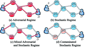
Figure 1: SPR in Different Regimes of Unknown Environments

III-C1 Adversarial Regime

In this regime, there is an attacker attacks (e.g., send interfering power and corrupt routers by worms, etc.) over all $n$ links such that link weights suffered completely (See Fig.1 (a)) that lead to metric value (e.g. link delay) loss. Note that the adversarial regime as a classic model of the well known non-stochastic MAB problem [11] implies that the attacker launches attack in every time slot. It is the most general setting and the other three regimes can be regarded as special cases of the adversarial regime.

Attack Model: Different attack philosophies will lead to different level of effectiveness. We focus on the following two type of jammers in the adversarial regime:

a) Oblivious attacker: an oblivious attacker attacks different links with different attacking strength as a result of different data rate reductions, which is independent of the past communication records it might have observed.

b) Adaptive attacker: an adaptive attacker selects its attacking strength on the targeted (sub)set of links by utilizing its past experience and observation of the previous communication records. It is very powerful and can infer the SPR protocol and can launch attacks with different level of strength over a subset of links or routers during a single time slot based on the historical monitoring records. As shown in a recent work [9], no bandit algorithm can guarantee a sublinear regret $o(t)$ against an adaptive adversary with unbounded memory, because the adaptive adversary can mimic the behavior of SPR protocol to attack, which leads to a linear regret (the attack can not be defended). Therefore, we consider a more practical $\theta$-memory-bounded adaptive adversary [9] model. It is an adversary constrained to loss functions that depends only on the $\theta+1$ most recent strategies.

III-C2 Stochastic Regime

In this regime, the transceiver is communicating over $n$ stochastic links as shown in Fig.1 (b). The link weights $\ell_{t}(e),\forall e\in 1,...,n$ of each link $e$ are sampled independently from an unknown distribution that depends on $e$, but not on $t$. We use $\mu_{e}=\mathbb{E}\left[{{\ell_{t}(e)}}\right]$ to denote the expected loss of link $e$. We define link $e$ as the best link if $\mu(e)={\min_{e^{\prime}}}\{{\mu(e^{\prime})}\}$ and suboptimal link otherwise; let $e^{*}$ denote some best link. For each link $e$, define the gap $\Delta(e)=\mu(e)-\mu({e^{*}})$; let $\Delta_{e}={\min_{e:\Delta(e)>0}}\left\{{\Delta(e)}\right\}$ denote the minimal gap of links. The regret can be rewritten as

$$R(t)=\sum\nolimits_{e=1}^{n}{\mathbb{E}\left[{{N_{t}}(e)}\right]}\Delta(e).$$ (2)

Note that we can calculate the regret either from the perspective of links $e\in 1,...,n$ or from the perspective of strategies $\textbf{i}\in\mathcal{P}$. However, because of the set of strategies (paths) grows exponentially with respect to $n$ and it does not exploit the link dependency between different strategies, we can calculate the regret from links, where tight regret bounds are achievable.

III-C3 Mixed Adversarial and Stochastic Regime

This regime assumes that the attacker only attacks $k_{a}$ out of $k$ active links at each time slot shown in Fig.1 (c). There is always a $k_{a}/k$ portion of links under adversarial attack while the other $(k-k_{a})/k$ portion is stochastically distributed.

Attack Model: We consider the same attack model as in the adversarial regime. The difference here is that the attacker only attacks a subset of links of size $k_{a}$ over the total $k$ links.

III-C4 Contaminated Stochastic Regime

The definition of the contaminated stochastic regime comes from many practical observations that only a few links (or routers) and time slots are exposed to adversary. In this regime, for the oblivious attacker, it selects some slot-link pairs $(t,e)$ as “locations” to attack before the SPR starts, while the remaining link weights are generated the same as in the stochastic regime. We can introduce and define the attacking strength parameter $\zeta\in[0,1/2)$. After certain $\tau$ timslots, for all $t>\tau$ the total number of contaminated locations of each suboptimal link up to time $t$ is $t\Delta(e)\zeta$ and the number of contaminated locations of each best link is $t\Delta_{e}\zeta$. We call a contaminated stochastic regime moderately contaminated, if $\zeta$ is at most $1/4$, we can prove that for all $t>\tau$ on the average over the stochasticity of the loss sequence the adversary can reduce the gap of every link by at most one half.

Algorithm 1 AOSPR-EXP3++: An MAB-based Algorithm for AOSPR

  Input: $n,k,t$, and See text for definition of $\eta_{t}$ and $\xi_{t}(e)$.

  Initialization: Set initial link losses $\forall e\in[1,n],\tilde{\ell}_{0}(e)=0$. Then the initial link and path weights $\forall e\in[1,n],w_{0}(e)=1$ and $\forall\textbf{i}\in[1,N],W_{0}(\textbf{i})=k$, respectively. ​

  Set: ​​ $\beta_{t}\!\!=\!\!\frac{1}{2}\sqrt{\frac{{\ln n}}{{tn}}}$; ${\varepsilon_{t}}\left(e\right)\!=\!\min\left\{{\frac{1}{{2n}},{\beta_{t}},{\xi_{t}}\left(e\right)}\right\},\forall e\in\left[{1,n}\right]$.

  for  time slot $t=1,2,...$ do

     1: The source selects a path $\mathbf{I}_{t}$ at random according to the probability $\rho_{t}(\textbf{i}),\forall\mathbf{i}\in\mathcal{P}$, with $\rho_{t}(\textbf{i})$ computed as follows:

$${\rho_{t}}(\textbf{i})=\left\{\begin{array}[]{l}\!\!\!\left({1-\sum\nolimits_{e=1}^{n}{{\varepsilon_{t}}(e)}}\right)\frac{{{w_{t-1}}\left(\textbf{i}\right)}}{{{W_{t-1}}}}+\!\sum\limits_{e\in\textbf{i}}{{\varepsilon_{t}}(e)}\ \emph{if}\ \textbf{i}\in\mathcal{C}\\ \!\!\!\left({1-\sum\nolimits_{e=1}^{n}{{\varepsilon_{t}}(e)}}\right)\frac{{{w_{t-1}}\left(\textbf{i}\right)}}{{{W_{t-1}}}}\ \quad\quad\quad\quad\ \text{\emph{if}}\ \textbf{i}\notin\mathcal{C}\end{array}\right.$$

     2: The source computes the probability ${{\tilde{\rho}}_{t}}(e),\forall e\in E$, as

$$\begin{array}[]{l}\!\!\!\!\!{{{\tilde{\rho}}_{t}}}(e)=\sum\nolimits_{\textbf{i}:e\in\textbf{i}}{{\rho_{t}}(\textbf{i})}=\left({1-\sum\nolimits_{e=1}^{n}{{\varepsilon_{t}}(e)}}\right)\frac{{\sum\nolimits_{\textbf{i}:e\in\textbf{i}}{{w_{t-1}}\left(\textbf{i}\right)}}}{{{W_{t-1}}}}\\ \quad\quad\quad\quad\quad\quad\quad\quad\ \ +\sum\nolimits_{e\in\textbf{i}}{{\varepsilon_{t}}(e)}\left|{\left\{{\textbf{i}\in\mathcal{C}:e\in\textbf{i}}\right\}}\right|.\end{array}$$

     3: Observe the suffered link loss $\ell_{t-1}(e),\forall e\in\textbf{I}_{t}$, and update its estimated value by ${\tilde{\ell}_{t}}(e)=\frac{{{\ell_{t}}(e)}}{{{{{\tilde{\rho}}_{t}}}(e)}},\forall e\in\textbf{I}_{t}$. Otherwise, ${\tilde{\ell}_{t}}(e)=0,\forall e\notin\textbf{I}_{t}$.

     4: The source updates all the weights as ${w_{t}}\left(e\right)={w_{t-1}}\left(e\right){e^{-\eta_{t}{{\tilde{\ell}}_{t}}(e)}}={e^{-\eta_{t}{{\tilde{L}}_{t}}(e)}}$ and ${{\bar{w}}_{t}}\left(\textbf{i}\right)=\prod\nolimits_{e\in\textbf{i}}{{w_{t}}(e)}={{\bar{w}}_{t-1}}\left(\textbf{i}\right){e^{-\eta_{t}{{\tilde{\ell}}_{t}}(\textbf{i})}}$, where ${{\tilde{L}}_{t}}(e)={{\tilde{L}}_{t-1}}(e)+{{\tilde{\ell}}_{t-1}}(e),{{\tilde{\ell}}_{t-1}}(e)=\sum\nolimits_{e\in\textbf{i}}{{{\tilde{\ell}}_{t-1}}(e)}$ and ${{\tilde{L}}_{t}}(\textbf{i})={{\tilde{L}}_{t-1}}(\textbf{i})+{{\tilde{\ell}}_{t-1}}(\textbf{i})$. The sum of weights of all strategies is calculated as ${W_{t}}=\sum\limits_{\textbf{i}\in\mathcal{P}}{{{\bar{w}}_{t}}\left(\textbf{i}\right)}.$

  end for

IV Single-Source Adaptive Optimal SPR

IV-A Coupled Probing and Routing

This section develops an SPR algorithm for a single source. The design philosophy is that the source collects the link delays of the previously chosen paths, based on which it can decide the next time slot routing strategy. The main difficulty is that it requires the algorithm to appropriately balance between exploitation and exploration. On the one hand, such an algorithm needs to keep exploring the best set of paths; on the other hand, it needs to exploit the already selected best set of paths so that they are not under utilized.

We describe Algorithm 1, namely AOSPR-EXP3++, a variant based on EXP3 algorithm, whose performance in the four regimes is proved to be asymptotically optimal. Our new algorithm uses the fact that when link delays of the chosen path are revealed, it also provides useful information about other paths with shared common links. During each time slot, we assign a link weight that is dynamically adjusted based on the link delays revealed to the source. The weight of a path is determined by the product of weights of all links. Our algorithm has two control parameters: the learning rate $\eta_{t}$ and the exploration parameter $\varepsilon_{t}(e)$ for each link $e$. To facilitate the adaptive and optimal SPR without the knowledge about the nature of the environments, the crucial innovation is the introduction of exploration parameter $\xi_{t}(e)$ into $\varepsilon_{t}(e)$ for each link $e$, which is tuned individually for each arm depending on the past observations.

Let $N$ denote the total number of strategies at the source side. A set of covering strategy is defined to ensure that each link is sampled sufficiently often. It has the property that for each link $e$, there is a strategy $\textbf{i}\in\mathcal{C}$ such that $e\in\textbf{i}$. Since there are only $n$ links and each strategy includes $k$ links, we set $|\mathcal{C}|=\lceil{\frac{n}{{{k}}}}\rceil$. As such, there is no-overlapping among different paths in the set of the covering strategy to maximize the covering range. The value $\sum\nolimits_{e\in\textbf{i}}{{\varepsilon_{t}}(e)}$ means the randomized exploration probability for each strategy $\textbf{i}\in\mathcal{C}$, which is the summation of each link $e$’s exploration probability ${\varepsilon_{t}}\left(e\right)$ that belongs to the strategy i. The introduction of $\sum\nolimits_{e\in\textbf{i}}{{\varepsilon_{t}}\left(e\right)}$ ensures $\rho_{t}(\textbf{i})\geq\sum\nolimits_{e\in\textbf{i}}{{\varepsilon_{t}}(e)}$ so that a mixture of exponential weight distribution and uniform distribution [14].

In the following discussion, we show that tuning only the learning rate $\eta_{t}$ is sufficient to control and obtain the regret of the AOSPR-EXP3++ in the adversarial regime, regardless of the choice of exploration parameter $\xi_{t}(e)$. Then we show that tuning only the exploration parameter $\xi_{t}(e)$ is sufficient to control the regret of AOSPR-EXP3++ in the stochastic regimes regardless of the choice of $\eta_{t}$, as long as $\eta_{t}\geq\beta_{t}$. To facilitate the AOSPR-EXP3++ algorithm without knowing about the nature of environments, we can apply the two control parameters simultaneously by setting $\eta_{t}=\beta_{t}$ and use the control parameter $\xi_{t}(e)$ in the stochastic regimes such that it can achieve the optimal “root-t” regret in the adversarial regime and almost optimal “logarithmic-t” regret in the stochastic regime (though with a suboptimal power in the logarithm).

IV-B Performance Results in Different Regimes

We present the regret performance of our proposed AOSPR-EXP3++ algorithm in different regimes as follows. The analysis involves with martingale theory and some special concentration inequalities, which are put in Section VII.

IV-B1 Adversarial Regime

We first show that tuning $\eta_{t}$ is sufficient to control the regret of AOSPR-EXP3++ in the adversarial regime, which is a general result that holds for all other regimes.

Theorem 1. Under the oblivious adversary, no matter how the status of the links change (potentially in an adversarial manner), for $\eta_{t}=\beta_{t}$ and any $\xi_{t}(e)\geq 0$, the regret of the AOSPR-EXP3++ algorithm for any $t$ satisfies

$$R(t)\leq 4{k}\sqrt{tn\ln n}.$$

Note that Theorem 1 attains the same result as in [8] in the adversarial regime for oblivious adversary, based on which we get result for the adaptive adversary in the following.

Theorem 2. Under the $\theta$-memory-bounded adaptive adversary, no matter how the status of the links change (potentially in an adversarial manner), for $\eta_{t}=\beta_{t}$ and any $\xi_{t}(e)\geq 0$, the regret of the AOSPR-EXP3++ algorithm for any $t$ satisfies

$$R(t)\leq(\theta+1){(4{k}\sqrt{n\ln n})^{\frac{2}{3}}}{t^{\frac{2}{3}}}+o({t^{\frac{2}{3}}}).$$

IV-B2 Stochastic Regime

Now we show that for any $\eta_{t}\geq\beta_{t}$, tuning the exploration parameters $\xi_{t}(e)$ is sufficient to control the regret of the algorithm in the stochastic regime. We also consider a different way of tuning the exploration parameters $\xi_{t}(e)$ for practical implementation considerations. We begin with an idealistic assumption that the gaps $\Delta(e),\forall e\in n$ is known, just to give an idea of what is the best result we can have and our general idea for all our proofs.

Theorem 3. Assume that the gaps $\Delta(e),\forall e\in n,$ are known. Let $t^{*}$ be the minimal integer that satisfies ${t^{*}(e)}\geq\frac{{4{c^{2}}n\ln{{({t^{*}(e)}\Delta{{(e)}^{2}})}^{2}}}}{{\Delta{{(e)}^{4}}\ln(n)}}$. For any choice of $\eta_{t}\geq{\beta_{t}}$ and any $c\geq 18$, the regret of the AOSPR-EXP3++ algorithm with $\xi_{t}(a)=\frac{{c\ln(t\Delta{{(e)}^{2}})}}{{t\Delta{{(e)}^{2}}}}$ in the stochastic regime satisfies

$$\begin{array}[]{l}R(t)\leq\sum\limits_{e=1,\Delta{(e)}>0}^{n}{O\left({\frac{{k\ln{{(t)}^{2}}}}{{\Delta{{(e)}}}}}\right)}+\sum\limits_{e=1,\Delta{(e)}>0}\Delta{{(e)}}t^{*}{{(e)}}\\ \hskip 19.91684pt={O\left({\frac{{kn\ln{{(t)}^{2}}}}{{\Delta_{e}{{}}}}}\right)}+\sum\limits_{e=1,\Delta{(e)}>0}\tilde{O}\left({\frac{n}{{\Delta{{(e)}^{3}}}}}\right).\end{array}$$

From the upper bound results, we note that the leading constants $k$ and $n$ are optimal and tight as indicated in CombUCB1 [16] algorithm. However, we have a factor of $\ln(t)$ worse of the regret performance than the optimal “logarithmic-t” regret as in [2, 4, 5], [12],[16], [24], where the performance gap is trivially negligible (See numerical results in Section VII).

A Practical Implementation by Estimating the Gap: Because of the gaps $\Delta(e),\forall e\in n$ can not be known in advance before running the algorithm. Next, we show a more practical result that uses the empirical gap as an estimate of the true gap. The estimation process can be performed in background for each link $e$ that starts from the running of the algorithm, i.e.,

$${{\hat{\Delta}}_{t}}(e)=\min\left\{{1,\frac{1}{t}\left({{\tilde{L}}_{t}}(e)-\mathop{\min}\limits_{e^{\prime}}({{\tilde{L}}_{t}}(e^{\prime}))\right)}\right\}.$$ (5)

This is a first algorithm that can be used in many real-world applications.

Theorem 4. Let $c\geq 18$ and $\eta_{t}\geq\beta_{t}$. Let $t^{*}$ be the minimal integer that satisfies $t^{*}\geq\frac{{4{c^{2}}\ln{{(t^{*})}^{4}}n}}{{\ln(n)}}$, and let ${t^{*}}(e)=\max\left\{{{t^{*}},\left\lceil{{e^{1/\Delta{{(e)}^{2}}}}}\right\rceil}\right\}$ and $t^{*}=max_{\{e\in n\}}t^{*}{{(e)}}$. The regret of the AOSPR-EXP3++ algorithm with ${\xi_{t}}(e)=\frac{{c{{\left({\ln t}\right)}^{2}}}}{{t{{\hat{\Delta}}_{t-1}}{{(e)}^{2}}}}$, termed as AOSPR-EXP3++${}^{\emph{AVG}}$, in the stochastic regime satisfies

$$\begin{array}[]{l}R(t)\leq\sum\limits_{e=1,\Delta{(e)}>0}^{n}{O\left({\frac{{k\ln{{(t)}^{3}}}}{{\Delta{{(e)}}}}}\right)}+\sum\limits_{e=1,\Delta{(e)}>0}^{n}\Delta{{(e)}}t^{*}{{(e)}}\\ \hskip 19.91684pt=O\left({\frac{{nk\ln{{(t)}^{3}}}}{{\Delta_{e}}}}\right)+nt^{*}.\end{array}$$

From the theorem, we observe that factor of another $ln(t)$ worse of the regret performance when compared to the idealistic case. Also, the additive constant $t^{*}$ in this theorem can be very large. However, our experimental results show that a minor modification of this algorithm achieves a comparable performance with ComUCB1 [16] in the stochastic regime.

IV-B3 Mixed Adversarial and Stochastic Regime

The mixed adversarial and stochastic regime can be regarded as a special case of mixing adversarial and stochastic regimes. Since there is always a jammer randomly attacking $k_{a}$ links out of the total $n$ links out of the total $k$ links constantly over time, we will have the following theorem for the AOSPR-EXP3++${}^{\emph{AVG}}$ algorithm, which is a much more refined regret performance bound than the general regret bound in the adversarial regime.

Theorem 5. Let $c\geq 18$ and $\eta_{t}\geq\beta_{t}$. Let $t^{*}$ be the minimal integer that satisfies $t^{*}\geq\frac{{4{c^{2}}\ln{{(t^{*})}^{4}}n}}{{\ln(n)}}$, and Let ${t^{*}}(e)=\max\left\{{{t^{*}},\left\lceil{{e^{1/\Delta{{(e)}^{2}}}}}\right\rceil}\right\}$ and $t^{*}=max_{\{e\in n\}}t^{*}{{(e)}}$. The regret of the AOSPR-EXP3++ algorithm with ${\xi_{t}}(e)=\frac{{c{{\left({\ln t}\right)}^{2}}}}{{t{{\hat{\Delta}}_{t-1}}{{(e)}^{2}}}}$, termed as AOSPR-EXP3++${}^{\emph{AVG}}$ under oblivious jamming attack, in the mixed stochastic and adversarial regime satisfies

$$\begin{array}[]{l}R(t)\leq\sum\limits_{e=1,\Delta{(e)}>0}^{n}{O\left({\frac{{(k-k_{a})\ln{{(t)}^{3}}}}{{\Delta{{(e)}}}}}\right)}+\sum\limits_{e=1,\Delta{(e)}>0}^{n}\Delta{{(e)}}t^{*}{{(e)}}\\ \hskip 28.45274pt+4{k_{a}}\sqrt{tn\ln n}\\ \hskip 19.91684pt=O\left({\frac{{{n}(k-k_{a})\ln{{(t)}^{3}}}}{{\Delta_{e}}}}\right)+nt^{*}+O\left({k_{a}}\sqrt{tn\ln n}\right).\end{array}$$

Note that the results in Theorem 5 have better regret performance than the results obtained by adversarial MAB as shown in Theorem 1 and the adaptive SPR algorithm in [7]. Similarly, we have the following result under adaptive adversarial attack.

Theorem 6. Let $c\geq 18$ and $\eta_{t}\geq\beta_{t}$. Let $t^{*}$ be the minimal integer that satisfies $t^{*}\geq\frac{{4{c^{2}}\ln{{(t^{*})}^{4}}n}}{{\ln(n)}}$, and Let ${t^{*}}(e)=\max\left\{{{t^{*}},\left\lceil{{e^{1/\Delta{{(e)}^{2}}}}}\right\rceil}\right\}$ and $t^{*}=max_{\{e\in n\}}t^{*}{{(e)}}$. The regret of the AOSPR-EXP3++ algorithm with ${\xi_{t}}(e)=\frac{{c{{\left({\ln t}\right)}^{2}}}}{{t{{\hat{\Delta}}_{t-1}}{{(e)}^{2}}}}$, termed as AOSPR-EXP3++${}^{\emph{AVG}}$ $\theta$-memory-bounded adaptive adversarial attack, in the mixed stochastic and adversarial regime satisfies

$$\begin{array}[]{l}\!\!R(t)\leq\sum\limits_{e=1,\Delta{(e)}>0}^{n}{O\left({\frac{{(k-k_{a})\ln{{(t)}^{3}}}}{{\Delta{{(e)}}}}}\right)}+\sum\limits_{e=1,\Delta{(e)}>0}^{n}\Delta{{(e)}}t^{*}{{(e)}}\\ \quad\quad+(\theta+1){(4{k_{a}}\sqrt{n\ln n})^{\frac{2}{3}}}{t^{\frac{2}{3}}}+o({t^{\frac{2}{3}}})\\ =O\left({\frac{{{(k-k_{a})}n\ln{{(t)}^{3}}}}{{\Delta_{e}}}}\right)+nt^{*}+O\left((\theta+1){({k_{a}}\sqrt{n\ln n})^{\frac{2}{3}}}{t^{\frac{2}{3}}}\right).\end{array}$$

IV-B4 Contaminated Stochastic Regime

We show that the algorithm AOSPR-EXP3++${}^{\emph{AVG}}$ can still retain “polylogarithmic-t” regret in the contaminated stochastic regime. The following is the result for the moderately contaminated stochastic regime.

Theorem 7. Under the setting of all parameters given in Theorem 3, for ${t^{*}}(e)=\max\left\{{{t^{*}},\left\lceil{{e^{4/\Delta{{(e)}^{2}}}}}\right\rceil}\right\}$, where $t^{*}$ is defined as before and $t_{3}^{*}=max_{\{e\in n\}}t^{*}{{(e)}}$, and the attacking strength parameter $\zeta\in[0,1/2)$ the regret of the AOSPR-EXP3++ algorithm in the contaminated stochastic regime that is contaminated after $\tau$ steps satisfies

$$\begin{array}[]{l}\!\!R(t)\leq\!\!\sum\limits_{e=1,\Delta{(e)}>0}^{n}\!\!\!\!{O\left({\frac{{k\ln{{(t)}^{3}}}}{{(1-2\zeta)\Delta{{(e)}}}}}\right)}\!\!+\!\!\sum\limits_{e=1,\Delta{(e)}>0}^{n}\!\!\!\!\Delta{{(e)}}\max\{t^{*}{{(e)}},\tau\}.\\ \!\hskip 19.91684pt={O\left({\frac{{nk\ln{{(t)}^{3}}}}{{(1-2\zeta)\Delta_{e}}}}\right)}+nt_{3}^{*}.\end{array}$$

If $\zeta\in(1/4,1/2)$, we find that the leading factor $1/(1-2\zeta)$ is very large, which is severely contaminated. Now, the obtained regret bound is not quite meaningful, which could be much worse than the regret performance in the adversarial regime for both oblivious and adaptive adversary.

V Accelerated AOSPR Algorithm

This section focuses on the accelerated learning by multi-path probing, cooperative learning between multiple source-destination pairs and other practical issues. All important proofs are put in Section VIII.

V-A Multi-Path Probing for Adaptive Online SPR

Intuitively, probing multiple paths simultaneously would offer the source more available information to make decisions, which results in faster learning and smaller regret value. At each time slot $t$, the source gets a budget $1\leq{M_{t}}\leq N$ and picks a subsect ${\mathcal{O}_{t}}\subseteq\left\{{1,...,N}\right\}$ of $M_{t}$ paths to probe and observe the link weights of these routes. Note that the links weights that belong to the un-probed set of paths $\mathcal{P}\setminus\mathcal{O}_{t}$ are still unrevealed. Accordingly, we have the probed and observed set of links $\tilde{\mathcal{O}}_{t}$ with the simple property $e\in\tilde{\mathcal{O}}_{t},\forall e\in\textbf{i}\in\mathcal{O}_{t}$. The proposed algorithm 2 is based on Algorithm 1 with $\omega_{t-1}(\textbf{i})=w_{t-1}(\textbf{i})/W_{t-1},\forall\textbf{i}\in\mathcal{P}$ and $\omega_{t-1}(e)=\sum\nolimits_{\textbf{i}:e\in\textbf{i}}w_{t-1}(e)/W_{t-1},\forall e\in E$. The probability $\varrho_{t}=(\varrho_{t}(\mathbf{1}),...,\varrho_{t}(\mathbf{N}))$ of each observed path is computed as

$$\!\!{\varrho_{t}}(\mathbf{i})={\rho_{t}}(\textbf{i})+\left({1-{\rho_{t}}(\textbf{i})}\right)\frac{{{M_{t}}-1}}{{{N}-1}},\ if\ \textbf{i}\ \in\mathcal{O}_{t},$$ (6)

where a mixture of the new exploration probability $(M_{t}-1)/(N-1)$ is introduced and $\rho_{t}(\textbf{i})$ is defined in (5). Similarly, the link probability ${\tilde{\varrho}}_{t}=({\tilde{\varrho}}_{t}({1})...,{\tilde{\varrho}}_{t}({n}))$ is computed as

$$\!\!{\tilde{\varrho}_{t}}(e)={\tilde{\rho}_{t}}(e)+\left({1-{\tilde{\rho}_{t}}(e)}\right)\frac{{{m_{t}}-1}}{{{n}-1}},\ if\ e\ \in\mathcal{\tilde{O}}_{t}.$$ (7)

Here, we have a link-level the new mixing exploration probability $(m_{t}-1)/(n-1)$ and $\tilde{\rho}_{t}(e)$ is defined in (6). The probing rate $m_{t}$ denotes the number of simultaneous probes at time slot $t$. Assume the link weights measured by different probes within the same time slot also satisfy the assumption in Section II-A. The mixing probability $(m_{t}-1)/(n-1)$ is informed by the source to all links along the probed and observed paths over a total of $n$ links of the probed path $M_{t}$ is a constant value for a network with fixed topology. The source needs to know the number of $n$ and gradually collect the value of $m_{t}$ over time. Thus, the algorithm faces the problems of “Cold-Start” and delayed feedback. The design of (6) and (7) and the proof of all results in this section are non-trivial tasks in our unified framework .

Algorithm 2 AOSPR-MP-EXP3++: Prediction with Multi-Path Probing

  Input: $M_{1},M_{2},...,$, such that $M_{t}\in\mathcal{P}$. Set $\beta_{t},{\varepsilon_{t}}\left(e\right),{\xi_{t}}\left(e\right)$ at in Alg. 1. $\forall\textbf{i}\in\mathcal{P},\tilde{L}_{0}(\textbf{i})=0$ and $\forall e\in E,\tilde{\ell}_{0}(e)=0$.

  for  time slot $t=1,2,...$ do

     1: Choose one path $H_{t}$ according to $\rho_{t}$ (5). Get advice $\pi_{t}^{H_{t}}$ as the selected path. Sample $M_{t}-1$ additional paths uniformly over $N$. Denote the set of sampled paths by $\mathcal{O}_{t}$, where $H_{t}\in\mathcal{O}_{t}$ and $|\mathcal{O}_{t}|=M_{t}$. Let $\mathds{1}_{t}^{h}=\mathds{1}_{\{h\in\mathcal{O}_{t}\}}$.

     2: Update the path probabilities $\varrho_{t}(\mathbf{i})$ according to (6). The loss of the observed path is

$${{\tilde{\ell}}_{t}}(\textbf{i})=\frac{{{{\ell}_{t}}(\mathbf{i})}}{\varrho_{t}(\mathbf{i})}\mathds{1}_{t}^{h},\forall\textbf{i}\in{\mathcal{O}_{t}}.$$ (8)

     3: Compute the probability of choosing each link ${{\tilde{\rho}}_{t}}(e)$ that belongs to the selected path according to (6).

     4: let $\mathds{1}(e)_{t}=\mathds{1}(e)_{e\in h\in\mathcal{O}_{t}}$. Update the link probabilities $\tilde{\varrho}_{t}(e)$ according to (7). The loss of the observed links are

$${{\tilde{\ell}}_{t}}(e)=\frac{{{{\ell}_{t}}(e)}}{{{\tilde{\varrho}}_{t}}(e)}\mathds{1}(e)_{t},\forall{e}\in{\tilde{\mathcal{O}}_{t}}.$$ (9)

     5: Updates all weights ${w_{t}}\left(e\right),{{\bar{w}}_{t}}\left(\textbf{i}\right),W_{t}$ as in Alg. 1.

  end for

The Performance Results of Multi-path Probing in the Four Regimes: If $m_{t}$ is a constant or lower bounded by $m$, we have the following results.

Theorem 8. Under the oblivious attack with the same setting of Theorem 1, the regret of the AOSPR-EXP3++ algorithm in the accelerated learning with probing rate $m$ satisfies

$$R(t)\leq 4{k}\sqrt{t\frac{n}{m}\ln n}.$$

Theorem 9. Under the $\theta$-memory-bounded adaptive attack with the same setting of Theorem 2, the regret of the AOSPR-EXP3++ algorithm in the accelerated learning with probing rate $m$ satisfies

$$R(t)\leq(\theta+1){(4{k}\sqrt{\frac{n}{m}\ln n})^{\frac{2}{3}}}{t^{\frac{2}{3}}}+o({t^{\frac{2}{3}}}).$$

We consider the practical implementation in the stochastic regime by estimating the gap as in the (5), and the result under accelerated learning is given as:

Theorem 10. With all other parameters hold as in Theorem 4, the regret of the AOSPR-EXP3++ algorithm with ${\xi_{t}}(e)=\frac{{c{{\left({\ln t}\right)}^{2}}}}{{mt{{\hat{\Delta}}_{t-1}}{{(e)}^{2}}}}$ in the accelerated learning with probing rate $m$, in the stochastic regime satisfies

$$\begin{array}[]{l}R(t)\leq\sum\limits_{e=1,\Delta{(e)}>0}^{n}{O\left({\frac{{k\ln{{(t)}^{3}}}}{{m\Delta{{(e)}}}}}\right)}+\sum\limits_{e=1,\Delta{(e)}>0}^{n}\Delta{{(e)}}t^{*}{{(e)}}\\ \hskip 19.91684pt=O\left({\frac{{nk\ln{{(t)}^{3}}}}{{m\Delta_{e}}}}\right)+nt^{*}.\end{array}$$

Theorem 11. With all other parameters hold as in Theorem 5, the regret of the AOSPR-EXP3++ algorithm with ${\xi_{t}}(e)=\frac{{c{{\left({\ln t}\right)}^{2}}}}{{mt{{\hat{\Delta}}_{t-1}}{{(e)}^{2}}}}$ under oblivious jamming attack in the accelerated learning with probing rate $m$, in the mixed stochastic and adversarial regime satisfies

$$\begin{array}[]{l}R(t)\leq\sum\limits_{e=1,\Delta{(e)}>0}^{n}{O\left({\frac{{(k-k_{a})\ln{{(t)}^{3}}}}{{m\Delta{{(e)}}}}}\right)}+\sum\limits_{e=1,\Delta{(e)}>0}^{n}\Delta{{(e)}}t^{*}{{(e)}}\\ \hskip 19.91684pt+4{k_{a}}\sqrt{t\frac{n}{m}\ln n}\\ \hskip 19.91684pt=O\left({\frac{{{n}(k-k_{a})\ln{{(t)}^{3}}}}{{m\Delta_{e}}}}\right)+nt^{*}+O\left({k_{a}}\sqrt{t\frac{n}{m}\ln n}\right).\end{array}$$

Theorem 12. With all other parameters hold as in Theorem 6, the regret of the AOSPR-EXP3++ algorithm with ${\xi_{t}}(e)=\frac{{c{{\left({\ln t}\right)}^{2}}}}{{mt{{\hat{\Delta}}_{t-1}}{{(e)}^{2}}}}$ under the $\theta$-memory-bounded adaptive attack in the accelerated learning with probing rate $m$, in the mixed stochastic and adversarial regime satisfies

$$\begin{array}[]{l}\!\!\!R(t)\leq\sum\limits_{e=1,\Delta{(e)}>0}^{n}{O\left({\frac{{(k-k_{a})\ln{{(t)}^{3}}}}{{m\Delta{{(e)}}}}}\right)}+\sum\limits_{e=1,\Delta{(e)}>0}^{n}\Delta{{(e)}}t^{*}{{(e)}}\\ \quad\quad+(\theta+1){(4{k_{a}}\sqrt{\frac{n}{m}\ln n})^{\frac{2}{3}}}{t^{\frac{2}{3}}}+o({t^{\frac{2}{3}}})\\ =O\left({\frac{{{n}(k-k_{a})\ln{{(t)}^{3}}}}{{m\Delta_{e}}}}\right)+nt^{*}+O\left({(\theta+1)({k_{a}}\sqrt{\frac{n}{m}\ln n})^{\frac{2}{3}}}{t^{\frac{2}{3}}}\right).\end{array}$$

Theorem 13. With all other parameters hold as in Theorem 7, the regret of the AOSPR-EXP3++ algorithm in the accelerated learning with probing rate $m$ in the contaminated stochastic regime satisfies

$$\begin{array}[]{l}\!\!\!R(t)\leq\!\!\!\!\sum\limits_{e=1,\Delta{(e)}>0}^{n}\!\!\!\!{O\left({\frac{{k\ln{{(t)}^{3}}}}{{(1-2\zeta)\Delta{{(e)}}}}}\right)}\!\!+\!\!\sum\limits_{e=1,\Delta{(e)}>0}^{n}\!\!\!\!\Delta{{(e)}}\max\{t^{*}{{(e)}},\tau\}.\\ \hskip 17.07182pt={O\left({\frac{{nk\ln{{(t)}^{3}}}}{{m(1-2\zeta)\Delta_{e}}}}\right)}+nt_{3}^{*}.\end{array}$$

V-B Multi-Source Learning for SPR Routing

So far we have focused on a single source-destination pair. Now, we turn to study the more practical multi-source learning with multiple source-destination pairs $\{1,...,S\}$ (set $S=m$ to ease comparison), which may also accelerate learning if sources can share information. Depending on the approach of information sharing, we consider two typical cases: coordinated probing and uncoordinated probing. Both cases assume the sources share link measurements. The difference is the selection of probing path is either centralized or distributed.

In the coordinated probing case, the probing path are selected globally either by a cluster head or different sources. We refer the algorithm as AOSPR-CP-EXP3++. Given total of $M_{t}$ source-destination pairs at time $t$, the $M_{t}$ probing paths are sequentially chosen which satisfies the probing rate of one path per source-destination pair. It is identical to the multi-path probing case except that now the candidate paths are not from one’s own path, but from all source-destination pairs. Thus, the same results hold as in the Theorem 8-Theorem 13.

Theorem 14. The regret upper bounds in all different regimes for AOSPR-CP-EXP3++ hold the same as in Theorem 8-Theorem 13.

In the uncoordinated probing case, the probing paths are selected in a distributed manner using AOSPR-EXP3++. We denote the algorithm as AOSPR-UP-EXP3++. As such, links are no longer evenly measured since some links may be covered by more source-destination pairs than others. By applying a linear program to estimate the low bound on the least probed link over time $t$, we have a scale factor $\bar{\kappa}$ that defines the dependency degree of overlapping paths. Then, we obtain the following result.

Theorem 15. The regret upper bounds in all different regimes for AOSPR-UP-EXP3++ are: if $\bar{\kappa}=1$, it is equivalent to the single source-destination pair case, the same results hold as in the Theorem 1-Theorem 7; if $\bar{\kappa}=m$, it is equivalent to the accelerated learning of multi-path probing case where the regret results hold by the substitution of $m$ by $\bar{\kappa}$ in the Theorem 8-Theorem 13.

V-C The Cold-Start and Delayed feedback Issues

V-C1 The Cold-Start Issue

Before the initialization of the algorithm, the source does not know the number of links $n$ and the simultaneous probed number of links $m_{t}$, which is demanded in the probing probability calculation in (7). Thus, the algorithm faces the “cold-start” problem. Note that the $N$ can be a complete collection of paths of the source, it must contain a set of covering strategy $\mathcal{C^{\prime}}$ where the whole links of the network is covered and the total number of links $n$ is acquirable. Let $\underline{M}=\min_{t}\{M_{1},M_{2},...,M_{t},...\}$ denote the minimal probed path from source over time. We have the following Corollary 16 that indicates how long it takes for the AOSPR-MP-EXP3++ algorithm to work normally.

Corollary 16. It takes at most $\frac{N}{\underline{M}}$ timslots for the AOSPR-MP-EXP3++ algorithm to finish the “Cold-Start” phase and start working normally.

Proof:

Denote the event of the probability that source node probes the paths uniformly over the $N$ possible paths at each time slot as $\rm{X}$ and the event ${Y}$ of the probability that the number of probed links over total of $n$ links. Take the following conditional probability we have $\mathbb{E}[X]=\mathbb{E}[X|Y]\mathbb{E}[Y]$, where $\mathbb{E}[X]=\frac{{\mathbb{E}[{M_{t}}]}}{N}$ and $\mathbb{E}[Y]=\frac{{\mathbb{E}[{m_{t}}]}}{n}$. Due to the potential dependency among different paths, $\mathbb{E}[X|Y]\leq 1$. Thus, $\mathbb{E}[Y]\leq\mathbb{E}[X]$, i.e., $\frac{{\mathbb{E}[{m_{t}}]}}{n}\leq\frac{{\mathbb{E}[{M_{t}}]}}{N}$, which indicates $\frac{N}{M_{t}}\geq\frac{n}{m_{t}},\forall t$. Since each link has probability $p=\frac{m_{t}}{n}$ to be probed at every time slot. According to the geometric distribution, the expected time that every link is probed is $\frac{1}{p}=\frac{n}{m_{t}}\leq\frac{N}{M_{t}}\leq\frac{N}{\underline{M}}$. This completes the proof. ∎

Nevertheless, for practical implementations, the accurate number of $m$ and $n$ is still hard to obtain. It often comes with errors in acquiring these two values. Hence, we need to know the sensitivity of deviations of the two true values on the regret performance. The result is summarized as follows.

Theorem 17. Given the deviation of observed values $m$ is $m_{\Delta}$ in (7), the upper bound of the deviated of regret $R_{m_{\Delta}}(t)$ with respect to the original $R(t)$ given its upper bound $\bar{R}(t)$
(a) in the adversarial regime is $-\frac{1}{2}{m_{\Delta}}\frac{n}{m}\bar{R}(t)$ and $-\frac{1}{3}{m_{\Delta}}\frac{n}{m}\bar{R}(t)$ for oblivious jammer and for adaptive adversary, respectively; (b) in the stochastic regime and contaminated regime are both $-\frac{1}{2}\frac{m_{\Delta}}{m}\bar{R}(t)$; (c) in the mixed adversarial and stochastic regime is $-\frac{1}{2}\frac{m_{\Delta}}{m}\bar{R}^{k-k_{a}}(t)-\frac{1}{2}{m_{\Delta}}\frac{n}{m}\bar{R}^{k_{a}}(t)$ for oblivious adversary and is $-\frac{1}{3}\frac{m_{\Delta}}{m}\bar{R}^{k-k_{a}}(t)-\frac{1}{2}{m_{\Delta}}\frac{n}{m}\bar{R}^{k_{a}}(t)$ for adaptive adversary, where $\bar{R}^{k-k_{a}}(t)$ and $\bar{R}^{k_{a}}(t)$ represents the upper bounds with $k-k_{a}$ and $k_{a}$ links in the stochastic regime and adversarial regime, respectively.
Given the deviation of observed values $n$ is $n_{\Delta}$ in (7), the upper bound of deviated of regret $R_{n_{\Delta}}(t)$ with respect to the original $R(t)$ given its upper bound $\bar{R}(t)$
(d) in the adversarial regime is $\frac{1}{2}{n_{\Delta}}\frac{n}{m}\frac{{m-1}}{{n-1}}\bar{R}(t)\cong\frac{1}{2}{n_{\Delta}}\bar{R}(t)$ and $\frac{1}{3}{n_{\Delta}}\frac{n}{m}\frac{{m-1}}{{n-1}}\bar{R}(t)\cong\frac{1}{3}{n_{\Delta}}\bar{R}(t)$ for oblivious jammer and for adaptive jammer, respectively; (e) in the stochastic regime and contaminated regime are both $\bar{R}_{\Delta}(t)=0$; (f) in the mixed adversarial and stochastic regime is $\frac{1}{2}{n_{\Delta}}\bar{R}^{k_{a}}(t)$ for oblivious adversary and is $\frac{1}{3}{n_{\Delta}}\bar{R}^{k_{a}}(t)$ for adaptive adversary.

From the theorem 17, we know that the regret in the adversarial regime is more sensitive to the deviation $m_{\Delta}$ than the deviation $n_{\Delta}$, which guides the design of the network to acquire accurate value of $m_{t}$ during the probing phase. For the stochastic regimes, we also see that the regret is more sensitive to the deviation $m_{\Delta}$ than the deviation $n_{\Delta}$. Moreover, the relative deviations on $R(t)$ stochastic regimes, i.e, $R_{m_{\Delta}}(t)/R(t)=\Theta(\frac{m_{\Delta}}{m})$ and $R_{n_{\Delta}}(t)/R(t)=0$ is much less (sensitive) than that in adversarial regimes, i.e., $R_{m_{\Delta}}(t)/R(t)=\Theta({m_{\Delta}}\frac{n}{m})$ and $R_{n_{\Delta}}(t)/R(t)=n_{\Delta}$. We see all these phenomena in the simulations.

V-C2 Delayed Feedback Issue

In the network with a large number of links, the link delay feedback to the source node will spend a lot of time, which is prohibitive in the realtime process. Therefore, there are variant delayed feedbacks of each link to the source. Moreover, if the path is switched in the middle of a long streaming transmission, the network SPR protocol needs a while to find the new optimal transmission rate, and the delay of the first few packets after the switch can be very large. In a nutshell, the delayed feedback issue is practically important, and we have the following results.

Theorem 18. Given the largest expected deviations of observed link delay $\tau^{*}$, the expected delayed-feedback regret $R_{d}(t)$ with respect to the original $R(t)$ (a) Assuming the delays depend only on time but not on links, in the oblivious adversarial regime is upper bounded by ${d_{t}}\mathbb{E}[R({\frac{t}{{{d_{t}}}}})]$, where ${d_{t}}=\min\{t,\tau_{t}^{*}+1\}$ and $\tau_{t}^{*}$ is the largest link delay at time $t$; (b) Assuming the delays to be independent of the rewards of the actions, in the stochastic regime and contaminated regime is upper bounded by $\mathbb{E}[R(t)]+\sum\nolimits_{e=1}^{n}{{\Delta_{e}}\mathbb{E}[\tau_{e,t}^{*}]}$.

VI The Computationally Efficient Implementation of the AOPSR-EXP3++ Algorithm

The implementation of algorithm $1$ requires the computation of probability distributions and storage of $N$ strategies, which is obvious to have a time and space complexity $O(n^{k_{\textbf{i}}})$ for a given path of length $k_{\textbf{i}}$. As the number of links increases, the number of path will become exponentially large, which is very hard to be scalable and results in low efficiency. To address this important problem, we propose a computationally efficient enhanced algorithm by utilizing the dynamic programming techniques, as shown in Algorithm 3. The key idea of the enhanced algorithm is to select links in the selected path one by one until $k_{\textbf{i}}$ links are chosen, instead of choosing a path from the large path space in each time slot.

We use $S\left({\bar{e},\bar{k}}\right)$ to denote the path set of which each path selects $\bar{k}$ links from $\bar{e},\bar{e}+1,\bar{e},...,n$. We also use $\bar{S}\left({\bar{e},\bar{k}}\right)$ to denote the path set of which each path selects $\bar{k}$ links from link $1,2,...,\bar{e}$. We define ${W_{t}}(\bar{e},\bar{k})=\sum\nolimits_{\textbf{i}\in S(\bar{e},\bar{k})}{\prod\nolimits_{e\in\textbf{i}}{{w_{t}}(e)}}$ and ${W_{t}}(\bar{e},\bar{k})=\sum\nolimits_{\textbf{i}\in\bar{S}(\bar{e},\bar{k})}{\prod\nolimits_{e\in\textbf{i}}{{w_{t}}(e)}},$ Note that they have the following properties:

$${W_{t}}(\bar{e},\bar{k})={W_{t}}(\bar{e}+1,\bar{k})+{w_{t}}(\bar{e}){W_{t}}(\bar{e}+1,\bar{k}-1),$$ (10)

$${W_{t}}(\bar{e},\bar{k})={W_{t}}(\bar{e}-1,\bar{k})+{w_{t}}(\bar{e}){W_{t}}(\bar{e}-1,\bar{k}-1),$$ (11)

which implies both ${W_{t}}(\bar{e},\bar{k})$ and ${\bar{W}_{t}}(\bar{e},\bar{k})$ can be calculated in $O(k_{r}n)$ (Letting ${W_{t}}(\bar{e},0)=1$ and $W(n+1,\bar{k})=\bar{W}(0,\bar{k})=0$) by using dynamic programming for all $1\leq\bar{e}\leq n$ and $1\leq\bar{k}\leq k_{\textbf{i}}$.

$$(1-\sum\nolimits_{e=1}^{n}{{\varepsilon_{t}}(e)})\frac{{\sum\nolimits_{k^{\prime}=0}^{{k_{\textbf{i}}}-1}{{{\bar{W}}_{t-1}}(e-1,k^{\prime}){w_{t-1}}(e){W_{t-1}}(e+1,{k_{\textbf{i}}}-k^{\prime}-1)}}}{{{W_{t-1}}(1,k^{\prime})}}\\ +\sum\limits_{e\in\textbf{i}}{\varepsilon_{t}}(e)\left|{\textbf{i}\in C:e\in\textbf{i}}\right|$$ (14)

In step 1, instead of drawing a path, we select links of the path one by one until a path is found. Here, we select links one by one in the increasing order of channel indices, i.e., we determine whether the link $1$ should be selected, and the link $2$, and so on. For any link $e$, if $k^{\prime}\leq k_{\textbf{i}}$ links have been chosen in link $1,..,e-1$, we select link $e$ with probability

$$\frac{{{w_{t-1}}(e){W_{t}}(e+1,{k_{\textbf{i}}}-k^{\prime}-1)}}{{{W_{t-1}}(e,{k_{\textbf{i}}}-k^{\prime})}}$$ (12)

and not select $e$ with probability $\frac{{{W_{t}}(e+1,{k_{\textbf{i}}}-k^{\prime}-1)}}{{{W_{t-1}}(e,{k_{\textbf{i}}}-k^{\prime})}}.$ Let $w(e)={w_{t-1}}(e)$ if link $e$ is selected in the path i; $w(e)=0$ otherwise. Obviously, $w(e)$ is actually the weight of $e$ in the path weight. In our algorithm, ${w_{t-1}}(e)=\prod\nolimits_{e=1}^{n}{w(e)}$. Let $c(e)=1$ if $e$ is selected in i; $c(e)=0$ otherwise. The term $\sum\nolimits_{e=1}^{\bar{e}}{c(e)}$ denotes the number of links chosen among link $1,2,...,\bar{e}$ in path i. In this implementation, the probability that a path i is selected, i.e., $\frac{{{w_{t-1}}(\textbf{i})}}{{{W_{t-1}}}}$, can be written as

$$\!\!\!\!\!\!\prod\limits_{\bar{e}=1}^{n}{\frac{{w(\bar{e}){W_{t-1}}(\bar{e}+1,{k_{\textbf{i}}}-\sum\nolimits_{e=1}^{\bar{e}}{c\left(e\right)})}}{{{W_{t-1}}(\bar{e},{k_{\textbf{i}}}-\sum\nolimits_{e=1}^{\bar{e}-1}{c\left(e\right)})}}}=\frac{{\prod\limits_{\bar{e}=1}^{n}{w(\bar{e})}}}{{{W_{t-1}}(1,{k_{\textbf{i}}})}}.$$ (13)

This probability is equivalent to that in Algorithm 1, which implies the implementation is correct. Because we do not maintain $w_{t}(\textbf{i})$, it is impossible to compute ${{{\tilde{\rho}}_{t}}}(e)$ as we have described in Algorithm 1. Then ${{{\tilde{\rho}}_{t}}}(e)$ can be computed within $O(nk_{r})$ as in Eq.(6) for each round.

Figure 2: Regret in Stochastic Regime

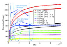
Figure 3: Regret in Contaminated Regime

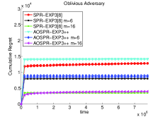
Figure 4: Regret in Adversarial Regime

For the exploration parameters $\varepsilon_{t}(e)$, since there are $k_{\textbf{i}}$ parameters of $\varepsilon_{t}(e)$ in the last term of Eqs. (14) below and there are $n$ links, the storage complexity is $O(kn)$. Similarly, we have the time complexity $O(knt)$ for the maintenance of exploration parameters $\varepsilon_{t}(e)$. Based on the above analysis, we can summarize the conclusions into the following theorem. Moreover, under delayed feedback, since the base algorithm has a memory requirement of $O(kn)$, the memory required by the delayed AUFH-EXP3++ by time step $t$ is upper bounded by $O(kn\tau_{t}^{*})$.

Theorem 19. The Algorithm 2 has polynomial time complexity $O(knt)$, space complexity $O(kn)$ and space complexity under the delayed feedback $O(kn\tau_{t}^{*})$ with respect to rounds $t$, parameters $k$ and $n$.

Besides, because of the link selection probability for $q_{t}(e)$ and the updated weights of Algorithm 2 equals to Algorithm 1, all the performance results in Section III and IV still hold for Algorithm 2.

Algorithm 3 A Computational Efficient Implementation of AOPSR-EXP3++

  Input: $n,k_{\textbf{i}},t$, and See text for definition of $\eta_{t}$ and $\xi_{t}(e)$.

  Initialization: Set initial link weight $w_{0}(e)=1,\forall e\in[1,n]$. Let $W_{t}(e,0)=1$ and $W(n+1,k^{\prime})=\bar{W}(0,k^{\prime})=0$ and compute $W_{0}(e,k^{\prime})$ and $\bar{W}_{0}(e,k^{\prime})$ follows Eqs. (10) and (11), respectively.

  for time slot $t=1,2,...$ do

     1: The source selects a link $e,\forall e\in[1,n]$ one by one according to the link’s probability distribution computed following Eq. (12) until a path with $k_{\textbf{i}}$ chosen links are selected.

     2: The source computes the probability $q_{t}(e),\forall e\in\left[{1,n}\right]$ according to Eq. (14).

     3: The source calculates the loss for channel $e$, $\ell_{t-1}(e),\forall e\in\textbf{i}_{t}$ based on the link loss $\ell_{t-1}(e)$. Compute the estimated loss $\tilde{\ell}_{t}(e),\forall e\in[1,n]$ as follows:

$${\tilde{\ell}_{t}}(e)=\left\{\begin{array}[]{l}\frac{{{\ell_{t}}(e)}}{{{q_{t}}(e)}}\quad\text{\emph{if channel}}e\in{\textbf{i}_{t}}\\ 0\ \ \quad\quad\emph{otherwise}.\end{array}\right.$$

     4: The source updates all channel weights as ${w_{t}}\left(e\right)={w_{t-1}}\left(e\right){e^{-\eta_{t}{{\tilde{\ell}}_{t}}(e)}}={e^{-\eta_{t}{{\tilde{L}}_{t}}(e)}},\forall e\in[1,n]$, and computes $W_{t}(e,k^{\prime})$ and $\bar{W}_{t}(e,k^{\prime})$ follows Eqs. (10) and (11), respectively.

  end for

VII Numerical and Simulation Results

We evaluate the performance of our online adaptive SPR algorithm using a wireless sensor network (WSN) adopting the IEEE 802.15 standard deployed on a university building. The trace contains QoS metrics of detailed link quality information, i.e., delay, goodput and packet loss rate, under an extensive set of parameter configurations are measured. The dataset close to 50 thousand parameter configurations were experimented and measurement data of more than 200 million packets were collected over a period of 6 months. Each sender-receiver is employed by a pair of TelosB nodes, each equipped with a TI CC2420 radio using the IEEE 802.15.4 stack implementation in TinyOS, which is placed in hallways of a five floor building. The WSN contains $16$ nodes, and there is line-of-sight path between the two nodes of a path at a specific distance, which was varied for different experiments ranging from 10 meters to 35 meters. Each node is forwarding packets under a particular stack parameter configuration, where the configuration set is finite.

The delay perceived by a packet mainly consists of two parts: queuing delay and service time delay, which are measured for every data packet. More specifically, it includes the ACK frame transmission time, retransmission duration, ACK maximal timeout if damage occurs by the adversarial attack, etc. To quantitatively answer how all the layer stack parameters contribute to the delay performance, there are four different types of datasets to emulate the following four typical regime of the environments: 1) the measured link quality data at night, where the link states distributions are benign and only affected by multi-path reflections from the walls; 2) the measured contaminated link quality data at daytime from $3:00pm-4:00pm$, when university students and employees walk most frequently in the hallway, which is a particularly harsh wireless environment; 3) the measured adversarial link quality, by the same type of TelosB nodes working under the same stack parameter configuration but sending garbage data to launch oblivious jamming attack during the run of the algorithm. The link delay labeled $N/A$ are replaced by $1111$ or $999$ in the dataset to indicate completed data packet loss; 4) the measured adversarial link quality under adaptive jamming attack, where the the algorithm is implemented by a set of $\theta$-memory jammers of our proposed AOSPR-EXP3++ algorithm. We omit the mixed adversarial and stochastic regime for brevity.

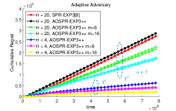
Figure 5: Regret in Adversarial Regime

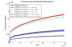
Figure 6: Centr. and Distr. Implementations

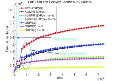
Figure 7: Cold Start and Delayed Feedback

All computations of collected datasets were conducted on an off-the-shelf desktop with dual $6$-core Intel i7 CPUs clocked at $2.66$Ghz. We make ten repetitions of each experiment to reduce the potential performance bias. The solid lines in the graphs represent the mean performance over the experiments and the dashed lines represents the mean plus on standard deviation (std) over the ten repetitions of the corresponding experiments. To show the advantage of our AOPSR-EXP3++ algorithms, we need to compare the performance of ours to other existing MAB based algorithms. They include: the EXP3 based SPR algorithm in [8], which is named as “SPR-EXP3”; the Upper-Confidence-Bound (UCB) based online SPR algorithm “OSPR” in [2] and their variations. We set all versions of our AOPSR-EXP3++ algorithms parameterized by ${\xi_{t}}(e)=\frac{{\ln(t{{\hat{\Delta}}_{t}}{{(e)}^{2}})}}{{32t{{\hat{\Delta}}_{t}}{{(e)}^{2}}}}$, where ${{{\hat{\Delta}}_{t}}(e)}$ is the empirical estimate of ${{{\Delta}_{t}}(e)}$ defined in (5).

In our first group of experiments in the stochastic regime (environment) as shown in Fig. 1, it is clear to see that AOPSR-EXP3++ enjoys almost the same (cumulative) regrets as OSPR [2] and has much lower regrets over time than the adversarial SPR-EXP3 [8]. We also see the significantly regrets reduction when accelerated learning ($m=6,16$) is employed for both OSPR and AOPSR-EXP3++.

In our second group of experiments in the moderately contaminated stochastic environment, there are several contaminated time slots as labeled in Fig. 3. In this case, the contamination is not fully adversarial, but drawn from a different stochastic model. Despite the corrupted rounds the AOPSR-EXP3++ algorithm successfully returns to the stochastic operation mode and achieves better results than SPR-EXP3 [8]. With light contaminations, the performance of OSPR in [2] is comparable to AOPSR-EXP3++, although it is not applicable here due to the i.i.d. assumption of OSPR.

We conducted the third group of experiments in the adversarial regimes. We studied the oblivious adversary case in Fig. 4. Due to the strong interference effect on each link and the arbitrarily changing feature of the jamming behavior, all algorithms experience very high accumulated regrets. It can be find that our AOPSR-EXP3++ algorithm will have close and slightly worst learning performance when compared to SPR-EXP3 [8], which confirms our theoretical analysis. Note that we do not implement stochastic MAB algorithms such as “OSPR” in [2], since it is inapplicable in this regime. Moreover, we studied the adaptive adversary case in Fig. 5. Compared with Fig. 4, the learning performance is much worse, which results in close to linear (but still sublinear) regret values, especially when the memory size of $\Theta$ is large. From the collected data, we see a 252% increase in the network delay under the adaptive adversary with $\Theta=4$ when compared to the oblivious adversary conditions. The value becomes 845% when $\Theta=20$, which shows the adaptive attacker is very hard to defend.

The centralized and distributed implementation of our cooperative learning AOSPR-EXP3++ algorithms are presented in Fig. 6. The sensitivity of the deviation of observed values $m$ and $n$ in stochastic and adversarial regimes are presented in Fig. 8. It is obvious to see the effects of $m_{\Delta}$ and $n_{\Delta}$ on the regret of AOSPR-EXP3++ in the stochastic regime is much smaller compared to the counterpart in the adversarial regimes. On average, we see a deviation of regret about 12% in the stochastic regime for the values of $m_{\Delta}$ and $n_{\Delta}$ show in Fig. 8, while the deviation of regret is about 126% in the adversarial regime. This indicated that our algorithm is more sensitive to the attacked environments than benign environments.

We conduct the “Cold-Start” and delayed feedback version of all algorithms in Fig. 7 in a general unknown environment that consists of data randomly mixed in all four regimes. The “Cold-Start” phase takes about $3\sim 20$ packets delivery timslots. Although it is hard to see the first 20 rounds on the plot, their effect on all the algorithms is clearly visible. For delayed feedback problem, we see a “quick jump” of regret for adversarial MAB algorithms (e.g., SPR-EXP3[8]) at initial rounds that confirms its multiplicative effect to $\tau^{*}$, while the relative small regret increase is seen for stochastic MAB algorithms (e.g., OSPR [2] and AOSPR-EXP3++) that confirms its additive effect to $\tau^{*}$.

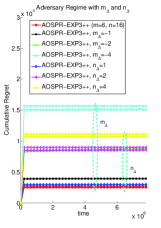
Figure 8: Sensitivity of $m$ and $n$ in Adver. and Stoc. Regimes

We also compared the averaged received data packets delay with different network sizes as shown in Fig. 9 for the mixed stochastic and adversarial regime under different number of links after a relative long period of learning rounds $n=7*10^{7}$. We can find that with the increasing of the network size, the learning performance of our AOSPR-EXP3++ is approaching the state-of-the-art algorithms OSPR [2] and SPR-EXP3[8] in the stochastic and adversarial regimes, which indicates its superior flexibility in large scale network deployments.

TABLE I: Computation Time Comparisons of Algorithm 1 and Algorithm 3

$(n,k)$
Alg. Ver. vs Comp. Time (micro seconds)	$(12,4)$	$(24,4)$	$(48,6)$	$(48,12)$	$(64,6)$	$(64,12)$	$(64,24)$
AOPSR-EXP3++: Algorithm1	46.1610	267.3351	819.7124	2622.1341	11087.0957	222376.0135	1868341.2324
AOPSR-EXP3++ Algorithm3	14.5137	29.1341	61.6366	157.6732	258.3622	456.1143	790.5101

With the increasing of the network size, we find that the learning performance of our AOSPR-EXP3++ is approaching the state-of-the-art algorithms OSPR [2] and SPR-EXP3[8] in the stochastic and adversarial regimes, which indicates its superior flexibility in large scale network deployments. Comparing the values of average received data packets delays of our AOSPR-EXP3++ to that of the classic algorithm SPR-EXP3, we see a $65.3\%$ improvements of the EE in average under different set of links $n=4,8,16,32,64$ under oblivious jamming attack, and a $124.8\%$ improvements under adaptive jamming attack. Moreover, to reach the same value of delay for the AOSPR-EXP3++ algorithm, the SPR-EXP3 takes a total of $n=12.8*10^{7}$ learning rounds. This indicates a $81.5\%$ improvement in the learning period of our proposed AOSPR-EXP3++ algorithm.

Moreover, we test the performance of the computational efficiency of our algorithms, where the computational time is compared in Table 1. From the results, we know that the computationally efficient version of the AOPSR-EXP3++ algorithm, i.e., Algorithm 3, takes about several hundreds of micro-seconds on average, while the original algorithm takes about several hundreds of seconds, which is prohibitive in practical implementations.

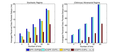
Figure 9: Delay Performance with Different Network Size

VIII Proofs of Regrets in Different Regimes for the Signal-Source AOSPR

We prove the theorems of the performance results in Section III in the order they were presented.

VIII-A The Adversarial Regimes

The proof of Theorem 1 borrows some of the analysis of EXP3 of the loss model in [10]. However, the introduction of the new mixing exploration parameter and the truth of link dependency as a special type of combinatorial MAB problem in the loss model makes the proof a non-trivial task, and we prove it for the first time.

Proof of Theorem 1.

Proof:

Note first that the following equalities can be easily verified: ${\mathbb{E}_{\textbf{i}\sim{\rho_{t}}}}{\tilde{\ell}_{t}}(\textbf{i})={\ell_{t}}({\textbf{I}_{t}}),{\mathbb{E}_{{\tilde{\ell}_{t}}\sim{\rho_{t}}}}{\ell_{t}}(\textbf{i})={\ell_{t}}(\textbf{i}),{\mathbb{E}_{\textbf{i}\sim{\rho_{t}}}}{\tilde{\ell}_{t}}{(\textbf{i})^{2}}=\frac{{{\ell_{t}}{{({\textbf{I}_{t}})}^{2}}}}{{{\rho_{t}}({\textbf{I}_{t}})}}$ and ${\mathbb{E}_{{\textbf{I}_{t}}\sim{\rho_{t}}}}\frac{1}{{{\rho_{t}}({\textbf{I}_{t}})}}=N$.

Then, we can immediately rewrite $R(t)$ and have

$$R(t)=\mathbb{E}_{t}\left[\sum\limits_{s=1}^{t}{{\mathbb{E}_{\textbf{i}\sim{p_{s}}}}{\tilde{\ell}_{s}}(\textbf{i})}-\sum\limits_{s=1}^{t}{{\mathbb{E}_{{I_{s}}\sim{p_{s}}}}{\tilde{\ell}_{s}}(\textbf{i})}\right].$$

The key step here is to consider the expectation of the cumulative losses ${\tilde{\ell}_{t}}(\textbf{i})$ in the sense of distribution $\textbf{i}\sim{\rho_{t}}$. Let ${\varepsilon_{t}}(\textbf{i})=\sum\nolimits_{e\in\textbf{i}}{{\varepsilon_{t}}(e)}$. However, because of the mixing terms of $\rho_{t}$, we need to introduce a few more notations. Let $u=({\underbrace{\sum\nolimits_{e\in 1}{{\varepsilon_{t}}(e)},...,\sum\nolimits_{e\in\textbf{i}}{{\varepsilon_{t}}(e)},...,\sum\nolimits_{e\in|\mathcal{C}|}{{\varepsilon_{t}}(e)}}_{\textbf{i}\in\mathcal{C}},\underbrace{0,...,0}_{\textbf{i}\notin\mathcal{C}}})$ be the distribution over all the strategies. Let ${\omega_{t-1}}=\frac{{{\rho_{t}}-u}}{{1-\sum\nolimits_{e}{{\varepsilon_{t}}(e)}}}$ be the distribution induced by AOSPR-EXP3++ at the time $t$ without mixing. Then we have:

$$\!\!\begin{array}[]{l}{\mathbb{E}_{\textbf{i}\sim{p_{s}}}}{{\tilde{\ell}}_{s}}(\textbf{i})=({1-\sum\nolimits_{e}{{\varepsilon_{s}}(e)}}){\mathbb{E}_{\textbf{i}\sim{\omega_{s-1}}}}{{\tilde{\ell}}_{s}}(\textbf{i})+{\varepsilon_{s}}(\textbf{i}){\mathbb{E}_{\textbf{i}\sim u}}{{\tilde{\ell}}_{s}}(\textbf{i})\\ \quad\quad\quad\quad\ \ =({1-\sum\nolimits_{e}{{\varepsilon_{s}}(e)}})(\frac{1}{{{\eta_{s}}}}\ln{\mathbb{E}_{\textbf{i}\sim{\omega_{s-1}}}}\exp(-{\eta_{s}}({{\tilde{\ell}}_{s}}(\textbf{i})\\ \quad\quad\quad\quad\quad\ -{\mathbb{E}_{\textbf{j}\sim{\omega_{s-1}}}}\tilde{\ell}_{t}(\textbf{j}))))\\ \quad\quad\quad\quad\quad\ -\frac{({1-\sum\nolimits_{e}{{\varepsilon_{s}}(e)}})}{{{\eta_{s}}}}\ln{\mathbb{E}_{\textbf{i}\sim{\omega_{s-1}}}}\exp(-{\eta_{s}}{{\tilde{\ell}}_{s}}(\textbf{i})))\\ \quad\quad\quad\quad\quad\ +{\mathbb{E}_{\textbf{i}\sim u}}{{\tilde{\ell}}_{t}}(\textbf{i}).\end{array}$$

Recall that for all the strategies, we have distribution $\omega_{t-1}=(\omega_{t-1}(1),...,\omega_{t-1}(N))$ with

$${\omega_{t-1}}(\textbf{i})=\frac{{\exp(-\eta_{t}{{\tilde{L}}_{t-1}}(\textbf{i}))}}{{\sum\nolimits_{j=1}^{N}{\exp(-\eta_{t}{{\tilde{L}}_{t-1}}(\textbf{j}))}}},$$ (16)

and for all the links, we have distribution $\omega_{t-1,e}=(\omega_{t-1,e}(1),...,\omega_{t-1,e}(n))$

$${\omega_{t-1,e}}(e^{\prime})=\frac{{\sum\nolimits_{\textbf{i}:e^{\prime}\in\textbf{i}}\exp(-\eta_{t}{{\tilde{L}}_{t-1}}(\textbf{i}))}}{{\sum\nolimits_{j=1}^{N}{\exp(-\eta_{t}{{\tilde{L}}_{t-1}}(\textbf{j}))}}}.$$ (17)

In the second step, we use the inequalities $lnx\leq x-1$ and $exp(-x)-1+x\leq x^{2}/2$, for all $x\geq 0$, and the fact that take expectations over $\textbf{j}\sim{\omega_{s-1}}$ and over $\textbf{i}\sim{\omega_{s-1}}$ are equivalent, to obtain:

$$\begin{array}[]{l}\ln{\mathbb{E}_{\textbf{i}\sim{\omega_{s-1}}}}\exp(-{\eta_{s}}({{\tilde{\ell}}_{s}}(\textbf{i})-{\mathbb{E}_{\textbf{j}\sim{\omega_{s-1}}}}{{\tilde{\ell}}_{s}}(\textbf{j})))\\ \quad\quad\quad=\ln{\mathbb{E}_{\textbf{i}\sim{\omega_{s-1}}}}\exp(-{\eta_{s}}{{\tilde{\ell}}_{s}}(\textbf{i}))+{\eta_{s}}{\mathbb{E}_{\textbf{i}\sim{\omega_{s-1}}}}{{\tilde{\ell}}_{s}}(\textbf{i})\\ \quad\quad\quad\leq{\mathbb{E}_{\textbf{i}\sim{\omega_{s-1}}}}({\exp(-{\eta_{s}}{{\tilde{\ell}}_{s}}(\textbf{i}))-1+{\eta_{s}}{{\tilde{\ell}}_{s}}(\textbf{i})})\\ \quad\quad\quad\leq{\mathbb{E}_{\textbf{i}\sim{\omega_{s-1}}}}\frac{{\eta_{s}^{2}{{\tilde{\ell}}_{s}}{{(\textbf{i})}^{2}}}}{2}.\end{array}$$

Take expectations over all random strategies of losses ${{\tilde{\ell}}_{s}}{(\textbf{i})^{2}}$, we have

$$\begin{array}[]{l}{\mathbb{E}_{t}}\left[{\mathbb{E}_{\textbf{i}\sim{w_{s}}}}{{\tilde{\ell}}_{s}}{(\textbf{i})^{2}}\right]={\mathbb{E}_{t}}\left[\sum\limits_{\textbf{i}=1}^{N}{{\omega_{s-1}}(\textbf{i}){{\tilde{\ell}}_{s}}{{(\textbf{i})}^{2}}}\right]\\ ={\mathbb{E}_{t}}\!\!\left[\sum\limits_{\textbf{i}=1}^{N}{{\omega_{s-1}}(\textbf{i}){{(\sum\limits_{e\in\textbf{i}}{{{\tilde{\ell}}_{s}}(e)})}^{2}}}\right]\leq{\mathbb{E}_{t}}\!\!\left[\sum\limits_{\textbf{i}=1}^{N}{{\omega_{s-1}}(\textbf{i}){k}\!\!\sum\limits_{e\in\textbf{i}}{{{\tilde{\ell}}_{s}}{{(e)}^{2}}}}\right]\\ =\!{\mathbb{E}_{t}}k\left[\!\sum\limits_{e=1}^{n}{{{\tilde{\ell}}_{s}}{{(e)}^{2}}}\!\!\!\!\sum\limits_{\textbf{i}\in{\mathcal{P}}:e\in\textbf{i}}\!\!\!{{\omega_{s-1}}(\textbf{i})}\right]\!=\!{k}{\mathbb{E}_{t}}\!\!\left[\!\sum\limits_{e^{\prime}=1}^{n}\!{{{\tilde{\ell}}_{s}}{{(e^{\prime})}^{2}}{\omega_{s-1,e}}(e^{\prime})}\right]\\ \end{array}$$

$$\begin{array}[]{l}={k}{\mathbb{E}_{s}}\left[{\sum\limits_{e^{\prime}=1}^{n}{{{\left({\frac{{{l_{t}}(e^{\prime})}}{{{{{\tilde{\rho}}_{s}}}(e^{\prime})}}{\mathds{1}_{s}}(e^{\prime})}\right)}^{2}}}{\omega_{s-1,e}}(e^{\prime})}\right]\\ \leq{k}{\mathbb{E}_{s}}\left[{\sum\limits_{e^{\prime}=1}^{n}{\frac{{{\omega_{s-1,e}}(e^{\prime})}}{{{{{\tilde{\rho}}_{s}}}{{(e^{\prime})}^{2}}}}{\mathds{1}_{s}}(e^{\prime})}}\right]={k}\sum\limits_{e^{\prime}=1}^{n}{\frac{{{\omega_{s-1,e}}(e^{\prime})}}{{{{{\tilde{\rho}}_{s}}}(e^{\prime})}}}\\ ={k}\sum\limits_{e^{\prime}=1}^{n}{\frac{{{\omega_{s-1,e}}(e^{\prime})}}{{\left({1-\sum\nolimits_{e}{{\varepsilon_{s}}(e)}}\right){\omega_{s-1,e}}(e^{\prime})+{{\sum\nolimits_{e\in\textbf{i}}{{\varepsilon_{s}}(e)}}}{{}}\left|{\left\{{\textbf{i}\in\mathcal{C}:e\in\textbf{i}}\right\}}\right|}}}\leq 2kn,\end{array}$$

where the last inequality follows the fact that $({1-\sum\nolimits_{e}{{\varepsilon_{t}}(e)}})\geq\frac{1}{2}$ by the definition of ${{\varepsilon_{t}}(e)}$.

In the third step, note that ${{\tilde{L}}_{0}}(\textbf{i})=0$. Let ${\Phi_{t}}(\eta)=\frac{1}{\eta}\ln\frac{1}{N}\sum\nolimits_{\textbf{i}=1}^{N}{\exp(-\eta{{\tilde{L}}_{t}}(\textbf{i}))}$ and ${\Phi_{0}}(\eta)=0$. The second term in (VIII-A) can be bounded by using the same technique in [10] (page 26-28). Let us substitute inequality (VIII-A) into (VIII-A), and then substitute (VIII-A) into equation (VIII-A) and sum over $t$ and take expectation over all random strategies of losses up to time $t$, we obtain

$$\begin{array}[]{l}{\mathbb{E}_{t}}\left[\sum\limits_{s=1}^{t}{\mathbb{E}_{\textbf{i}\sim{p_{s}}}}{{\tilde{\ell}}_{s}}(\textbf{i})\right]\leq kn\!\sum\limits_{s=1}^{t}\eta_{s}+\frac{{\ln N}}{\eta_{t}}+\!\!\sum\limits_{s=1}^{t}\!{\mathbb{E}_{\textbf{i}\sim u}}{{\tilde{\ell}}_{s}}(\textbf{i})\\ \hskip 46.94687pt+{\mathbb{E}_{t}}\left[\sum\limits_{s=1}^{t-1}{{\Phi_{s}}({\eta_{s+1}})-{\Phi_{s}}({\eta_{s}})}\right]+\sum\limits_{s=1}^{t}{{\mathbb{E}_{{I_{s}}\sim{p_{s}}}}{\tilde{\ell}_{s}}(\textbf{i})}.\end{array}$$

Then, we get

$$R(t)=\mathbb{E}_{t}\sum\limits_{s=1}^{t}{{\mathbb{E}_{\textbf{i}\sim{p_{s}}}}{\tilde{\ell}_{s}}(\textbf{i})}-\mathbb{E}_{t}\sum\limits_{s=1}^{t}{{\mathbb{E}_{{I_{s}}\sim{p_{s}}}}{\tilde{\ell}_{s}}(\textbf{i})}$$

$$\hskip 19.91684pt\leq kn\!\sum\limits_{s=1}^{t}\eta_{s}+\frac{{\ln N}}{\eta_{t}}+\sum\limits_{s=1}^{t}\!{\mathbb{E}_{\textbf{i}\sim u}}{{\tilde{\ell}}_{s}}(\textbf{i})$$

$$\hskip 19.91684pt\mathop{\leq}\limits^{(a)}kn\!\sum\limits_{s=1}^{t}\eta_{s}+\frac{{\ln N}}{\eta_{t}}+k\sum\limits_{s=1}^{t}{\sum\limits_{e=1}^{n}{{\varepsilon_{s}}(e)}}$$

$$\hskip 19.91684pt\mathop{\leq}\limits^{(b)}2kn\!\sum\limits_{s=1}^{t}\eta_{s}+\frac{{\ln N}}{\eta_{t}}$$

$$\hskip 19.91684pt\mathop{\leq}\limits^{(c)}2kn\!\sum\limits_{s=1}^{t}\eta_{s}+k\frac{{\ln n}}{\eta_{t}}.$$

Note that, the inequality $(a)$ holds by setting ${{\tilde{\ell}}_{s}}(\textbf{i})=k,\forall\textbf{i},s$, and the upper bound is $k\sum\nolimits_{\textbf{i}\in C}{{\sum\nolimits_{e\in\textbf{i}}{{\varepsilon_{t}}(e)}}}=k\sum\nolimits_{s=1}^{t}{\sum\nolimits_{e=1}^{n}{{\varepsilon_{s}}(e)}}$. The inequality $(b)$ holds, because of, for every time slot $t$, $\eta_{t}\geq{\varepsilon_{t}}(e)$. The inequality $(c)$ is due to the fact that $N\leq n^{k}$. Setting $\eta_{t}=\beta_{t}$, we prove the theorem. ∎

Proof of Theorem 2.

Proof:

To defend against the $\theta$-memory-bounded adaptive adversary, we need to adopt the idea of the mini-batch protocol proposed in [9]. We define a new algorithm by wrapping AOSPR-EXP3++ with a mini-batching loop [26]. We specify a batch size $\tau$ and name the new algorithm AOSPR-EXP3++_τ. The idea is to group the overall time slots $1,...,t$ into consecutive and disjoint mini-batches of size $\tau$. It can be viewed that one signal mini-batch as a round (time slot) and use the average loss suffered during that mini-batch to feed the original AOSPR-EXP3++. Note that our new algorithm does not need to know $m$, which only appears as a constant as shown in Theorem 2. So our new AOSPR-EXP3++_τ algorithm still runs in an adaptive way without any prior about the environment. If we set the batch $\tau={(4{k}\sqrt{n\ln n})^{-\frac{1}{3}}}{t^{{}^{\frac{1}{3}}}}$ in Theorem 2 of [9], we can get the regret upper bound in our Theorem 2. ∎

VIII-B The Stochastic Regime

Our proofs are based on the following form of Bernstein’s inequality with minor improvement as shown in [15].

Lemma 1. (Bernstein’s inequality for martingales). Let $X_{1},...,X_{m}$ be martingale difference sequence with respect to filtration $\mathcal{F}=(\mathcal{F}_{\textbf{i}})_{1\leq k\leq m}$ and let $Y_{k}=\sum\nolimits_{j=1}^{k}{{X_{j}}}$ be the associated martingale. Assume that there exist positive numbers $\nu$ and $c$, such that $X_{j}\leq c$ for all $j$ with probability $1$ and $\sum\nolimits_{k=1}^{m}{\mathbb{E}\left[{{{\left({{X_{k}}}\right)}^{2}}|{\mathcal{F}_{k-1}}}\right]}\leq\nu$ with probability 1.

$$\mathbb{P}[{Y_{m}}>\sqrt{2\nu b}+\frac{{cb}}{3}]\leq{e^{-b}}.$$

We also need to use the following technical lemma, where the proof can be found in [15].

Lemma 2. For any $c>0$, we have $\sum\nolimits_{t=0}^{\infty}{{e^{-c\sqrt{t}}}}=O\left({\frac{2}{{{c^{2}}}}}\right)$.

To obtain the tight regret performance for AOSPR-EXP3++, we need to study and estimate the number of times each of link is selected up to time $t$, i.e., $N_{t}(e)$. We summarize it in the following lemma.

Lemma 3. Let $\left\{{{{\underline{\varepsilon}}_{t}}(e)}\right\}_{t=1}^{\infty}$ be non-increasing deterministic sequences, such that ${{\underline{\varepsilon}}_{t}}(e)\leq{{\varepsilon}_{t}}(e)$ with probability $1$ and ${{\underline{\varepsilon}}_{t}}(e)\leq{{\varepsilon}_{t}}(e^{*})$ for all $t$ and $e$. Define $\nu_{t}(e)=\sum\nolimits_{s={1}}^{t}\frac{1}{{{k\underline{\varepsilon}}_{s}}(e)}$, and define the event $\mathcal{E}^{e}_{t}$

$${t\Delta(e)-({{{\tilde{L}}_{t}}(e)-{{\tilde{L}}_{t}}({e^{*}})})}$$

$$\hskip 36.98866pt\leq{\sqrt{2({\nu_{t}}(e)+{\nu_{t}}({e^{*}})){b_{t}}}+\frac{{{(1/k+0.25)}{b_{t}}}}{{3k{\underline{\varepsilon}_{t}}({e^{*}})}}}\hskip 8.5359pt(\mathcal{E}^{e}_{t}).$$

Then for any positive sequence $b_{1},b_{2},...,$ and any $t^{*}\geq 2$ the number of times link $e$ is played by AOSPR-EXP3++ up to round $t$ is bounded as:

$$\begin{array}[]{l}\mathbb{E}[{N_{t}}(e)]\leq\left({{t^{*}}-1}\right)+\sum\limits_{s={t^{*}}}^{t}{{e^{-{b_{s}}}}}+k\sum\limits_{s={t^{*}}}^{t}{{\varepsilon_{s}}(e){\mathds{1}_{\{\mathcal{E}^{e}_{t}\}}}}\\ \hskip 45.52458pt+\sum\limits_{s={t^{*}}}^{t}{{e^{-{\eta_{s}}{h_{s-1}}(e)}}},\end{array}$$

where

$$\begin{array}[]{l}{h_{t}}(e)=t\Delta(e)-\sqrt{2t{b_{t}}\left({\frac{1}{{{k}{{\underline{\varepsilon}}_{t}}(e)}}+\frac{1}{{{k}{{\underline{\varepsilon}}_{t}}({e^{*}})}}}\right)}-\frac{{(\frac{1}{4}+\frac{1}{k}){b_{t}}}}{{3{{\underline{\varepsilon}}_{t}}({e^{*}})}}.\end{array}$$

Proof:

Note that the elements of the martingale difference sequence $\{{\Delta(e)-({{\tilde{\ell}}_{t}}(e)-{{\tilde{\ell}}_{t}}({e^{*}}))}\}_{t=1}^{\infty}$ by $\max\{\Delta(e)+{{\tilde{\ell}}_{t}}({e^{*}})\}={\frac{1}{{{k}{{\underline{\varepsilon}}_{t}}({e^{*}})}}}+1$. Since ${{{\underline{\varepsilon}}_{t}}({e^{*}})}\leq{{{\varepsilon}_{t}}({e^{*}})}\leq 1/(2n)\leq 1/4$, we can simplify the upper bound by using ${\frac{1}{{{{k\underline{\varepsilon}}_{t}}({e^{*}})}}}+1\leq\frac{{(\frac{1}{4}+\frac{1}{k})}}{{{{\underline{\varepsilon}}_{t}}({e^{*}})}}$.

We further note that

$$\begin{array}[]{l}\sum\limits_{s=1}^{t}{{\mathbb{E}_{s}}\left[{{(\Delta(e)-({{\tilde{\ell}}_{s}}(e)-{{\tilde{\ell}}_{s}}({e^{*}})))}^{2}}\right]}\\ \hskip 31.2982pt\leq\sum\limits_{s=1}^{t}{{\mathbb{E}_{s}}\left[{{({{\tilde{\ell}}_{s}}(e)-{{\tilde{\ell}}_{s}}({e^{*}}))}^{2}}\right]}\\ \hskip 31.2982pt=\sum\limits_{s=1}^{t}{\left({{\mathbb{E}_{s}}\left[({{\tilde{\ell}}_{s}}{{(e)}^{2}}\right]+{E_{s}}\left[({{\tilde{\ell}}_{s}}{{({e^{*}})}^{2}}\right]}\right)}\\ \hskip 31.2982pt\leq\sum\limits_{s=1}^{t}\left({\frac{1}{{{q_{s}}(e)}}+\frac{1}{{{q_{s}}({e^{*}})}}}\right)\\ \hskip 31.2982pt\mathop{\leq}\limits^{(a)}\sum\limits_{s=1}^{t}{\left({\frac{1}{{k{\varepsilon_{s}}(e)}}+\frac{1}{{k{\varepsilon_{s}}({e^{*}})}}}\right)}\\ \hskip 31.2982pt\leq\sum\limits_{s=1}^{t}{\left({\frac{1}{{k{{\underline{\varepsilon}}_{s}}(e)}}+\frac{1}{{k{{\underline{\varepsilon}}_{s}}({e^{*}})}}}\right)}={\nu_{t}}(e)+{\nu_{t}}({e^{*}})\end{array}$$

with probability $1$. The above inequality (a) is due to the fact that ${{\tilde{\rho}}_{t}}(e)\geq\sum\nolimits_{e\in\textbf{i}}{{\varepsilon_{t}}(e)}\left|{\left\{{\textbf{i}\in\mathcal{C}:e\in\textbf{i}}\right\}}\right|$. Since each $e$ only belongs to one of the covering strategies $\textbf{i}\in\mathcal{C}$, $\left|{\left\{{\textbf{i}\in\mathcal{C}:e\in\textbf{i}}\right\}}\right|$ equals to 1 at time slot $t$ if link $e$ is selected. Thus, ${{\tilde{\rho}}_{t}}(e)\geq\sum\nolimits_{e\in\textbf{i}}{{\varepsilon_{t}}(e)}=k{\varepsilon_{t}}(e)$.

Let $\mathcal{\bar{E}}_{t}^{e}$ denote the complementary of event $\mathcal{E}_{t}^{e}$. Then by the Bernstein’s inequality $\mathbb{P}[\mathcal{\bar{E}}_{t}^{e}]\leq e^{-b_{t}}$. The number of times the link $e$ is selected up to round $t$ is bounded as:

$$\begin{array}[]{l}\mathbb{E}[{N_{t}}(e)]=\sum\limits_{s=1}^{t}{\mathbb{P}[A_{s}=e]}\\ \hskip 40.00006pt=\sum\limits_{s=1}^{t}{\mathbb{P}[A_{s}=e|\mathcal{E}_{s-1}^{e}]P[\mathcal{E}_{s-1}^{e}]}\\ \hskip 50.00008pt+\mathbb{P}[A_{s}=e|\overline{\mathcal{E}_{s-1}^{e}}]P[\overline{\mathcal{E}_{s-1}^{e}}]\\ \hskip 40.00006pt\leq\sum\limits_{s=1}^{t}{\mathbb{P}[A_{s}=e|\mathcal{E}_{s-1}^{e}]}{\mathds{1}_{\{\mathcal{E}_{s-1}^{e}\}}}+\mathbb{P}[\overline{\mathcal{E}_{s-1}^{S}}]\\ \hskip 40.00006pt\leq\sum\limits_{s=1}^{t}{\mathbb{P}[A_{s}=e|\mathcal{E}_{s-1}^{e}]}{\mathds{1}_{\{\mathcal{E}_{s-1}^{e}\}}}+{e^{-{b_{s-1}}}}.\end{array}$$

We further upper bound ${\mathbb{P}[A_{s}=e|\mathcal{E}_{s-1}^{e}]}{\mathds{1}_{\{\mathcal{E}_{s-1}^{e}\}}}$ as follows:

$$\begin{array}[]{l}\mathbb{P}{[A_{s}=e|{\cal\mathcal{E}}_{s-1}^{e}]}{\mathds{1}_{\{{\cal\mathcal{E}}_{s-1}^{e}\}}}={{{\tilde{\rho}}_{s}}}(e){\mathds{1}_{\{{\cal\mathcal{E}}_{s-1}^{e}\}}}\\ \hskip 40.00006pt\leq({\omega_{s-1}}(e)+k{\varepsilon_{s}}(e)){\mathds{1}_{\{{\cal\mathcal{E}}_{s-1}^{e}\}}}\\ \hskip 40.00006pt=({k\varepsilon_{s}}(e)+\frac{{\sum\nolimits_{\textbf{i}:e\in\textbf{i}}{{w_{s-1}}\left(\textbf{i}\right)}}}{{{W_{s-1}}}}){\mathds{1}_{\{{\cal\mathcal{E}}_{s-1}^{e}\}}}\\ \hskip 40.00006pt=({k\varepsilon_{s}}(e)+\frac{{\sum\nolimits_{\textbf{i}:e\in\textbf{i}}{{e^{-{\eta_{s}}{\tilde{L}_{s-1}}(\textbf{i})}}}}}{{\sum\nolimits_{\textbf{i}=1}^{N}{{e^{-{\eta_{s}}{\tilde{L}_{s-1}}(\textbf{i})}}}}}){\mathds{1}_{\{{\cal\mathcal{E}}_{s-1}^{e}\}}}\\ \hskip 40.00006pt\mathop{\leq}\limits^{(a)}({k\varepsilon_{s}}(e)+{e^{-{\eta_{s}}\left({{{\tilde{L}}_{s-1}}(\textbf{i})-{{\tilde{L}}_{s-1}}({\textbf{i}^{*}})}\right)}}){\mathds{1}_{\{{\cal\mathcal{E}}_{s-1}^{e}\}}}\\ \hskip 40.00006pt\mathop{\leq}\limits^{(b)}({k\varepsilon_{s}}(e)+{e^{-{\eta_{t}}\left({{{\tilde{L}}_{s-1}}(e)-{{\tilde{L}}_{s-1}}({e^{*}})}\right)}}){\mathds{1}_{\{{\cal\mathcal{E}}_{s-1}^{e}\}}}\\ \hskip 40.00006pt\mathop{\leq}\limits^{(c)}k{\varepsilon_{s}}(e){\mathds{1}_{\{{\cal\mathcal{E}}_{s-1}^{e}\}}}+{e^{-{\eta_{s}}{h_{s-1}}(e)}}.\end{array}$$

The above inequality (a) is due to the fact that link $e$ only belongs to one chosen path i in $t-1$, inequality (b) is because the cumulative regret of each path is great than the cumulative regret of each link that belongs to the path, and the last inequality (c) we used the fact that $\frac{t}{{{{\underline{\varepsilon}}_{t}}(e)}}$ is a non-increasing sequence ${\upsilon_{t}}(e)\leq\frac{t}{{{{k\underline{\varepsilon}}_{t}}(e)}}$. Substitution of this result back into the computation of $\mathbb{E}[{N_{t}}(e)]$ completes the proof. ∎

Proof of Theorem 3.

Proof:

The proof is based on Lemma 3. Let $b_{t}=ln(t\Delta(e)^{2})$ and ${{{\underline{\varepsilon}}_{t}}(e)}={{{\varepsilon}_{t}}(e)}$. For any $c\geq 18$ and any $t\geq t^{*}$, where $t^{*}$ is the minimal integer for which ${t^{*}}\geq\frac{{4{c^{2}}n\ln{{({t^{*}}\Delta{{(e)}^{2}})}^{2}}}}{{\Delta{{(e)}^{4}}\ln(n)}}$, we have

$$\begin{array}[]{l}{h_{t}}(e)=t\Delta(e)-\sqrt{2t{b_{t}}\left({\frac{1}{{k{\varepsilon_{t}}(e)}}+\frac{1}{{k{\varepsilon_{t}}({e^{*}})}}}\right)}-\frac{{\left({\frac{1}{4}+\frac{1}{k}}\right){b_{t}}}}{{3{\varepsilon_{t}}({e^{*}})}}\\ \hskip 24.29996pt\geq t\Delta(e)-2\sqrt{\frac{{t{b_{t}}}}{{k{\varepsilon_{t}}(e)}}}-\frac{{\left({\frac{1}{4}+\frac{1}{k}}\right){b_{t}}}}{{3{\varepsilon_{t}}(e)}}\\ \hskip 24.29996pt=t\Delta(e)(1-\frac{2}{{\sqrt{kc}}}-\frac{{\left({\frac{1}{4}+\frac{1}{k}}\right)}}{{3c}})\\ \hskip 24.29996pt\mathop{\geq}\limits^{(a)}t\Delta(e)(1-\frac{2}{{\sqrt{c}}}-\frac{{1.25}}{{3c}})\geq\frac{1}{2}t\Delta(e).\end{array}$$

The above inequality (a) is due to the fact that $(1-\frac{2}{{\sqrt{kc}}}-\frac{{\left({\frac{1}{4}+\frac{1}{k}}\right)}}{{3c}})$ is an increasing function with respect to $k(k\geq 1)$. Plus, as indicated in work [16], by a bit more sophisticated bounding $c$ can be made almost as small as 2 in our case. By substitution of the lower bound on $h_{t}(e)$ into Lemma 3, we have

$$\begin{array}[]{l}\!\!\!\mathbb{E}[{N_{t}}(e)]\leq{t^{*}}+\frac{{\ln(t)}}{{\Delta{{(e)}^{2}}}}+k\frac{{c\ln{{(t)}^{2}}}}{{\Delta{{(e)}^{2}}}}+\sum\limits_{s=1}^{t}\!\!\left(\!{{e^{-\frac{{\Delta(e)}}{4}\sqrt{\frac{{(s-1)ln(n)}}{n}}}}}\!\right)\\ \hskip 35.00005pt\leq k\frac{{c\ln{{(t)}^{2}}}}{{\Delta{{(e)}^{2}}}}+\frac{{\ln(t)}}{{\Delta{{(e)}^{2}}}}+O(\frac{{{n}}}{{\Delta{{(e)}^{2}}}})+{t^{*}},\end{array}$$

where lemma 3 is used to bound the sum of the exponents. In addition, please note that $t^{*}$ is of the order $O(\frac{{kn}}{{\Delta{{(e)}^{4}}\ln(n)}})$. ∎

Proof of Theorem 4.

Proof:

The proof is based on the similar idea of Theorem 2 and Lemma 3. Note that by our definition ${{\hat{\Delta}}_{t}}(e)\leq 1$ and the sequence ${\underline{\varepsilon}_{t}}(e)={\underline{\varepsilon}_{t}}=\min\{\frac{1}{{2n}},{\beta_{t}},\frac{{c\ln{{(t)}^{2}}}}{t}\}$ satisfies the condition of Lemma 3. Note that when ${\beta_{t}}\geq\frac{{c\ln{{(t)}^{2}}}}{t}\}$, i.e., for $t$ large enough such that $t\geq\frac{{4{c^{2}}\ln{{(t)}^{4}}n}}{{\ln(n)}}$, we have ${\underline{\varepsilon}_{t}}=\frac{{c\ln{{(t)}^{2}}}}{t}$. Let $b_{t}=ln(t)$ and let $t^{*}$ be large enough, so that for all $t\geq t^{*}$ we have $t\geq\frac{{4{c^{2}}\ln{{(t)}^{4}}n}}{{\ln(n)}}$ and $t\geq e^{\frac{1}{\Delta(e)^{2}}}$. With these parameters and conditions on hand, we are going to bound the rest of the three terms in the bound on $\mathbb{E}[N_{t}(e)]$ in Lemma 3. The upper bound of $\sum\nolimits_{s={t^{*}}}^{t}{{e^{-{b_{s}}}}}$ is easy to obtain. For bounding $k\sum\nolimits_{s={t^{*}}}^{t}{{\varepsilon_{s}}(e){\mathds{1}_{\{\mathcal{E}_{s-1}^{e}\}}}}$, we note that $\mathcal{E}_{t}^{e}$ holds and for $c\geq 18$ we have

$$\begin{array}[]{l}{{\hat{\Delta}}_{t}}(e)\geq\frac{1}{t}({{\tilde{L}}_{t}}(e)-\mathop{\max}\limits_{e^{\prime}}({{\tilde{L}}_{t}}(e^{\prime})))\geq\frac{1}{t}({{\tilde{L}}_{t}}(e)-{{\tilde{L}}_{t}}({e^{*}}))\\ \hskip 24.29996pt\geq\frac{1}{t}{h_{t}}(e)=\frac{1}{t}\left({t\Delta(e)-2\sqrt{\frac{{t{b_{t}}}}{{k{{\underline{\varepsilon}}_{t}}}}}-\frac{{(\frac{1}{4}+\frac{1}{k}){b_{t}}}}{{3{{\underline{\varepsilon}}_{t}}}}}\right)\\ \end{array}$$

$$\begin{array}[]{l}\hskip 24.29996pt=\frac{1}{t}\left({t\Delta(e)-\frac{{2t}}{{\sqrt{ck\ln(t)}}}-\frac{{(\frac{1}{4}+\frac{1}{k})t}}{{3c\ln(t)}}}\right)\\ \hskip 24.29996pt\mathop{\geq}\limits^{(a)}\frac{1}{t}\left({t\Delta(e)-\frac{{2t}}{{\sqrt{c\ln(t)}}}-\frac{{1.25t}}{{3c\ln(t)}}}\right)\\ \hskip 24.29996pt\mathop{\geq}\limits^{(b)}\Delta(e)\left({1-\frac{2}{{\sqrt{c}}}-\frac{{1.25}}{{3c}}}\right)\geq\frac{1}{2}\Delta(e),\end{array}$$

where the inequality (a) is due to the fact that $\frac{1}{t}(t\Delta(e)-\frac{2t}{\sqrt{ck\ln(t)}}-\frac{(\frac{1}{4}+\frac{1}{k})t}{3c\ln(t)})$ is an increasing function with respect to $k(k\geq 1)$ and the inequality (b) due to the fact that for $t\geq t^{*}$ we have $\sqrt{ln(t)}\geq 1/\Delta(e).$ Thus,

$${\varepsilon_{n}}(e){\mathds{1}_{\{\mathcal{E}_{n-1}^{e}\}}}\leq\frac{{c{{\left({\ln t}\right)}^{2}}}}{{t{{\hat{\Delta}}_{t}}{{(e)}^{2}}}}\leq\frac{{4{c^{2}}{{\left({\ln t}\right)}^{2}}}}{{t\Delta{{(e)}^{2}}}}$$

and $k\sum\nolimits_{s={t^{*}}}^{t}{{\varepsilon_{s}}(e){\mathds{1}_{\{\mathcal{E}_{n-1}^{e}\}}}}=O\left({\frac{{k\ln{{\left(t\right)}^{3}}}}{{\Delta{{(e)}^{2}}}}}\right)$. Finally, for the last term in Lemma 3, we have already get $h_{t}(e)\geq\frac{1}{2}\Delta(e)$ for $t\geq t^{*}$ as an intermediate step in the calculation of bound on ${{{\hat{\Delta}}_{t}}(e)}$. Therefore, the last term is bounded in a order of $O(\frac{{{n}}}{{\Delta{{(e)}^{2}}}})$. Use all these results together we obtain the results of the theorem. Note that the results holds for any $\eta_{t}\geq\beta_{t}$. ∎

VIII-C Mixed Adversarial and Stochastic Regime

Proof of Theorem 5.

Proof:

The proof of the regret performance in the mixed adversarial and stochastic regime is simply a combination of the performance of the AOSPR-EXP3++${}^{\emph{AVG}}$ algorithm in adversarial and stochastic regimes. It is very straightforward from Theorem 1 and Theorem 3. ∎

Proof of Theorem 6.

Proof:

Similar as above, the proof is very straightforward from Theorem 2 and Theorem 3. ∎

VIII-D Contaminated Stochastic Regime

Proof of Theorem 7.

Proof:

The key idea of proving the regret bound under moderately contaminated stochastic regime relies on how to estimate the performance loss by taking into account the contaminated pairs. Let $\mathds{1}_{t,e}^{\star}$ denote the indicator functions of the occurrence of contamination at location $(t,e)$, i.e., $\mathds{1}_{t,e}^{\star}$ takes value $1$ if contamination occurs and $0$ otherwise. Let $m_{t}(e)=\mathds{1}_{t,e}^{\star}\tilde{\ell}_{t}(e)+(1-\mathds{1}_{t,e}^{\star})\mu(e)$. If either base arm $e$ was contaminated on round $t$ then $m_{t}(e)$ is adversarially assigned a value of loss that is arbitrarily affected by some adversary, otherwise we use the expected loss. Let ${Z_{t}}(e)=\sum\nolimits_{s=1}^{t}{{m_{t}}(e)}$ then $\left({{Z_{t}}({e})-{Z_{t}}(e^{*})}\right)-\left({{{\tilde{L}}_{t}}({e})-{{\tilde{L}}_{t}}(e^{*})}\right)$ is a martingale. After $\tau$ steps, for $t\geq\tau$,

$$\begin{array}[]{l}\left({{Z_{t}}({e})-{Z_{t}}(e^{*})}\right)\geq t\min\{\mathds{1}_{t,e}^{\star},\mathds{1}_{t,e^{*}}^{\star}\}({\tilde{\ell}_{t}}(e)-{\tilde{\ell}_{t}}({e^{*}}))\\ \hskip 60.00009pt+t\min\{1-\mathds{1}_{t,e}^{\star},1-\mathds{1}_{t,e^{*}}^{\star}\}(\mu({e})-\mu(e^{*}))\\ \hskip 36.0001pt\geq-\zeta t\Delta(e)+(t-\zeta t\Delta(e))\Delta(e)\geq(1-2\zeta){t\Delta(e)}.\end{array}$$

Define the event $\mathcal{Z}_{t}^{e}$:

$$(1-2\zeta)t\Delta(e)-\left({{{\tilde{L}}_{t}}({e})-{{\tilde{L}}_{t}}(e^{*})}\right)\leq 2\sqrt{{\nu_{t}}{b_{t}}}+\frac{{\left({\frac{1}{4}+\frac{1}{k}}\right){b_{t}}}}{{3{{\underline{\varepsilon}}_{t}}}},$$

where ${\underline{\varepsilon}}_{t}$ is defined in the proof of Theorem 3 and $\nu_{t}=\sum\nolimits_{s=1}^{t}{\frac{1}{{{{k\underline{\varepsilon}}_{t}}}}}$. Then by Bernstein’s inequality $\mathbb{P}[\mathcal{Z}_{t}^{e}]\leq e^{-b_{t}}$. The remanning proof is identical to the proof of Theorem 3.

For the regret performance in the moderately contaminated stochastic regime, according to our definition with the attacking strength $\zeta\in[0,1/4]$, we only need to replace $\Delta(e)$ by $\Delta(e)/2$ in Theorem 5. ∎

IX Proof of Regret for Accelerated AOSPR Algorithm

We prove the theorems of the performance results in Section IV in the order they were presented.

IX-A Accelerated Learning in Adversarial Regime

The proof the Theorem 8 requires the following Lemma from Lemma 7 [19]. We restate it for completeness.

Lemma 4. For any probability distribution $\tilde{\omega}$ on $\{1,...,n\}$ and any $m\in[1,n]$:

$$\sum\limits_{e=1}^{n}{\frac{{\tilde{\omega}(e)(n-1)}}{{\tilde{\omega}(e)(n-m)+m-1}}\leq\frac{n}{m}}.$$

Proof of Theorem 8.

Proof:

Note first that the following equalities can be easily verified: ${\mathbb{E}_{\textbf{i}\sim{\varrho_{t}}}}{\tilde{\ell}_{t}}(\textbf{i})={\ell_{t}}({\textbf{I}_{t}}),{\mathbb{E}_{{\tilde{\ell}_{t}}\sim{\varrho_{t}}}}{\ell_{t}}(\textbf{i})={\ell_{t}}(\textbf{i}),{\mathbb{E}_{\textbf{i}\sim{\varrho_{t}}}}{\tilde{\ell}_{t}}{(\textbf{i})^{2}}=\frac{{{\ell_{t}}{{({\textbf{I}_{t}})}^{2}}}}{{{\varrho_{t}}({\textbf{I}_{t}})}}$ and ${\mathbb{E}_{{\textbf{I}_{t}}\sim{\varrho_{t}}}}\frac{1}{{{\varrho_{t}}({\textbf{I}_{t}})}}=N$.

Then, we can immediately rewrite $R(t)$ and have

$$R(t)=\mathbb{E}_{t}\left[\sum\limits_{s=1}^{t}{{\mathbb{E}_{\textbf{i}\sim{\rho_{s}}}}{\tilde{\ell}_{s}}(\textbf{i})}-\sum\limits_{s=1}^{t}{{\mathbb{E}_{{\textbf{I}_{s}}\sim{\rho_{s}}}}{\tilde{\ell}_{s}}(\textbf{i})}\right].$$

The key step here is to consider the expectation of the cumulative losses ${\tilde{\ell}_{t}}(\textbf{i})$ in the sense of distribution $\textbf{i}\sim{\varrho_{t}}$. Let ${\varepsilon_{t}}(\textbf{i})=\sum\nolimits_{e\in\textbf{i}}{{\varepsilon_{t}}(e)}$. However, because of the mixing terms of $\varrho_{t}$, we need to introduce a few more notations. Let $\varphi_{s}=({\underbrace{\sum\nolimits_{e\in 1}{{\varepsilon_{t}}(e)},...,\sum\nolimits_{e\in\textbf{i}}{{\varepsilon_{t}}(e)},...,\sum\nolimits_{e\in|\mathcal{C}|}{{\varepsilon_{t}}(e)}}_{\textbf{i}\in\mathcal{C}},\underbrace{0,...,0}_{\textbf{i}\notin\mathcal{C}}})$ be the distribution over all the strategies. Let ${\omega_{t-1}}=\frac{{{\rho_{t}}-u}}{{1-\sum\nolimits_{e}{{\varepsilon_{t}}(e)}}}$ be the distribution induced by AOSPR-EXP3++ at the time $t$ without mixing. Then we have:

$$\!\!\begin{array}[]{l}\!\!{\mathbb{E}_{\textbf{i}\sim{\rho_{s}}}}{{\tilde{\ell}}_{s}}(\textbf{i})=({1-\sum\nolimits_{e}{{\varepsilon_{s}}(e)}}){\mathbb{E}_{\textbf{i}\sim{\omega_{s-1}}}}{{\tilde{\ell}}_{s}}(\textbf{i})+\varepsilon_{s}(\textbf{i}){\mathbb{E}_{\textbf{i}\sim u}{\tilde{\ell}}_{s}(\textbf{i})}\\ \ \quad\quad\quad\ \ =({1-\sum\nolimits_{e}{{\varepsilon_{s}}(e)}})(\frac{1}{{{\eta_{s}}}}\ln{\mathbb{E}_{\textbf{i}\sim{\omega_{s-1}}}}\exp(-{\eta_{s}}({{\tilde{\ell}}_{s}}(\textbf{i})\\ \quad\quad\quad\quad\quad\ -{\mathbb{E}_{\textbf{j}\sim{\omega_{s-1}}}}\tilde{\ell}_{t}(\textbf{j}))))\\ \quad\quad\quad\quad\quad\ -\frac{({1-\sum\nolimits_{e}{{\varepsilon_{s}}(e)}})}{{{\eta_{s}}}}\ln{\mathbb{E}_{\textbf{i}\sim{\omega_{s-1}}}}\exp(-{\eta_{s}}{{\tilde{\ell}}_{s}}(\textbf{i})))\\ \quad\quad\quad\quad\quad\ +\varepsilon_{s}(\textbf{i}){\mathbb{E}_{\textbf{i}\sim u}{\tilde{\ell}}_{s}(\textbf{i})}.\end{array}$$

In the second step, by similar arguments as in the proof of Theorem 1, we have:

$$\begin{array}[]{l}\ln{\mathbb{E}_{\textbf{i}\sim{\omega_{s-1}}}}\exp(-{\eta_{s}}({{\tilde{\ell}}_{s}}(\textbf{i})-{\mathbb{E}_{\textbf{j}\sim{\omega_{s-1}}}}{{\tilde{\ell}}_{s}}(\textbf{j})))\\ \quad\quad\quad=\ln{\mathbb{E}_{\textbf{i}\sim{\omega_{s-1}}}}\exp(-{\eta_{s}}{{\tilde{\ell}}_{s}}(\textbf{i}))+{\eta_{s}}{\mathbb{E}_{\textbf{j}\sim{\omega_{s-1}}}}{{\tilde{\ell}}_{s}}(\textbf{j})\\ \quad\quad\quad\leq{\mathbb{E}_{\textbf{i}\sim{\omega_{s-1}}}}({\exp(-{\eta_{s}}{{\tilde{\ell}}_{s}}(\textbf{i}))-1+{\eta_{s}}{{\tilde{\ell}}_{s}}(\textbf{i})})\\ \quad\quad\quad\leq{\mathbb{E}_{\textbf{i}\sim{\omega_{s-1}}}}\frac{{\eta_{s}^{2}{{\tilde{\ell}}_{s}}{{(\textbf{i})}^{2}}}}{2}.\end{array}$$

Take expectations over all random strategies of losses ${{\tilde{\ell}}_{s}}{(\textbf{i})^{2}}$, we have

$$\begin{array}[]{l}\!\!\!{\mathbb{E}_{t}}\left[{\mathbb{E}_{\textbf{i}\sim{\omega_{s-1}}}}{{\tilde{\ell}}_{s}}{(\textbf{i})^{2}}\right]={\mathbb{E}_{t}}\left[\sum\limits_{\textbf{i}=1}^{N}{{\omega_{s-1}}(\textbf{i}){{\tilde{\ell}}_{s}}{{(\textbf{i})}^{2}}}\right]\\ \!\!\!\!={\mathbb{E}_{t}}\!\!\left[\sum\limits_{\textbf{i}=1}^{N}{{\omega_{s-1}}(\textbf{i}){{(\sum\limits_{e\in\textbf{i}}{{{\tilde{\ell}}_{s}}(e)})}^{2}}}\right]\leq{\mathbb{E}_{t}}\!\!\left[\sum\limits_{\textbf{i}=1}^{N}{{\omega_{s-1}}(\textbf{i}){k}\!\!\sum\limits_{e\in\textbf{i}}{{{\tilde{\ell}}_{s}}{{(e)}^{2}}}}\right]\\ \!\!\!\!=\!{\mathbb{E}_{t}}k\left[\!\sum\limits_{e=1}^{n}{{{\tilde{\ell}}_{s}}{{(e)}^{2}}}\!\!\!\!\sum\limits_{\textbf{i}\in{\mathcal{P}}:e\in\textbf{i}}\!\!\!{{\omega_{s-1}}(\textbf{i})}\right]\!=\!{k}{\mathbb{E}_{t}}\!\!\left[\!\sum\limits_{e^{\prime}=1}^{n}\!{{{\tilde{\ell}}_{s}}{{(e^{\prime})}^{2}}{\omega_{s-1,e}}(e^{\prime})}\right]\\ \!\!\!\!={k}{\mathbb{E}_{t}}\left[{\sum\limits_{e=1}^{n}{{{\left({\frac{{{l_{s}}(e)}}{{{{{\tilde{\varrho}}_{s}}}(e)}}{\mathds{1}_{s}}(e)}\right)}^{2}}}{\tilde{\omega}_{s-1}}(e)}\right]\\ \!\!\!\!\leq{k}{\mathbb{E}_{t}}\left[{\sum\limits_{e=1}^{n}{\frac{{{\tilde{\omega}_{s-1}}(e)}}{{{{{\tilde{\varrho}}_{s}}}{{(e)}^{2}}}}{\mathds{1}_{s}}(e)}}\right]={k}\sum\limits_{e=1}^{n}{\frac{{{\tilde{\omega}_{s-1}}(e)}}{{{{{\tilde{\varrho}}_{s}}}(e)}}}\\ \!\!\!\!={k}\!\!\sum\limits_{e=1}^{n}\!\!{\frac{{{\tilde{\omega}_{s-1}}(e)}}{{{\tilde{\rho}_{s}}(e)+(1-{\tilde{\rho}_{s}}(e))\frac{{{m_{s}}-1}}{{{n}-1}}}}}\mathop{\leq}\limits^{(a)}{k}\!\!\sum\limits_{e=1}^{n}\!\!{\frac{{2\tilde{\rho}_{s}}(e)}{{{\tilde{\rho}_{t}}(e)+(1-{\tilde{\rho}_{s}}(e))\frac{{{m_{s}}-1}}{{{n}-1}}}}}\\ \mathop{\leq}\limits^{(b)}2k\frac{n}{m},\end{array}$$

where the above inequality $(a)$ follows the fact that $({1-\sum\nolimits_{e}{{\varepsilon_{t}}(e)}})\geq\frac{1}{2}$ by the definition of ${{\varepsilon_{t}}(e)}$ and the equality (6) and the above inequality $(b)$ follows the Lemma 4. Note that ${\varphi_{s-1}}(e)=\sum\nolimits_{e\in\textbf{i}}{{\varepsilon_{t}}(e)}\left|{\left\{{\textbf{i}\in\mathcal{C}:e\in\textbf{i}}\right\}}\right|,\forall e\in[1,n]$ Take expectations over all random strategies of losses ${{\tilde{\ell}}_{s}}{(\textbf{i})}$ with respective to distribution $u$, we have

$$\begin{array}[]{l}{\mathbb{E}_{t}}\left[{\mathbb{E}_{\textbf{i}\sim{\varphi_{s}}}}{{\tilde{\ell}}_{s}}{(\textbf{i})}\right]={\mathbb{E}_{t}}\left[\sum\limits_{\textbf{i}=1}^{N}{{\varphi_{s}}(\textbf{i}){{\tilde{\ell}}_{s}}{{(\textbf{i})}}}\right]\\ ={\mathbb{E}_{t}}\!\!\left[\sum\limits_{\textbf{i}=1}^{N}{{\varphi_{s}}(\textbf{i}){{(\sum\limits_{e\in\textbf{i}}{{{\tilde{\ell}}_{s}}(e)})}}}\right]\leq{\mathbb{E}_{t}}\!\!\left[\sum\limits_{\textbf{i}=1}^{N}{{\varphi_{s}}(\textbf{i})(\sum\limits_{e\in\textbf{i}}{{{\tilde{\ell}}_{s}}{{(e)})}}}\right]\\ =\!{\mathbb{E}_{t}}\left[\!\sum\limits_{e=1}^{n}{{{\tilde{\ell}}_{s}}{{(e)}}}\!\!\!\!\sum\limits_{\textbf{i}\in{\mathcal{P}}:e\in\textbf{i}}\!\!\!{{\varphi_{s}}(\textbf{i})}\right]\!=\!{}{\mathbb{E}_{t}}\!\!\left[\!\sum\limits_{e^{\prime}=1}^{n}\!{{{\tilde{\ell}}_{s}}{{(e^{\prime})}}{\varphi_{s}}(e^{\prime})}\right]\\ \leq{k}{\mathbb{E}_{t}}\left[{\sum\limits_{e^{\prime}=1}^{n}{\frac{{\varphi_{s}}(e^{\prime})}{{{{{\tilde{\rho}}_{s}}}{{(e^{\prime})}}}}{\mathds{1}_{s}}(e^{\prime})}}\right]={k}\sum\limits_{e^{\prime}=1}^{n}{\frac{{\varphi_{s}}(e^{\prime})}{{{{{\tilde{\rho}}_{s}}}(e^{\prime})}}}\\ ={k}\sum\limits_{e^{\prime}=1}^{n}{\frac{{\varphi_{s}}(e^{\prime})}{{\tilde{\rho}_{s}}(e)+(1-{\tilde{\rho}_{s}}(e))\frac{{{m_{s}}-1}}{{{n}-1}}}}\\ \mathop{\leq}\limits^{(a)}{k}\sum\limits_{e^{\prime}=1}^{n}{\frac{{\tilde{\rho}_{s}}(e)}{{\tilde{\rho}_{s}}(e)+(1-{\tilde{\rho}_{s}}(e))\frac{{{m_{s}}-1}}{{{n}-1}}}}\leq 2k\frac{n}{m},\end{array}$$

where the above inequality $(a)$ is because ${\tilde{\rho}_{t}}(e)\geq{\varphi_{s-1}}(e)$.

In the third step, note that ${{\tilde{L}}_{0}}(\textbf{i})=0$. Let ${\Phi_{t}}(\eta)=\frac{1}{\eta}\ln\frac{1}{N}\sum\nolimits_{\textbf{i}=1}^{N}{\exp(-\eta{{\tilde{L}}_{t}}(\textbf{i}))}$ and ${\Phi_{0}}(\eta)=0$. The second term in (IX-A) can be bounded by using the same technique in [10] (page 26-28). Let us substitute inequality (IX-A) into (IX-A), and then substitute (IX-A) into equation (IX-A) and sum over $t$ and take expectation over all random strategies of losses up to time $t$, we obtain

$$\begin{array}[]{l}{\mathbb{E}_{t}}\left[\sum\limits_{s=1}^{t}{\mathbb{E}_{\textbf{i}\sim{\rho_{s}}}}{{\tilde{\ell}}_{s}}(\textbf{i})\right]\leq kn\!\sum\limits_{s=1}^{t}\eta_{s}+\frac{{\ln N}}{\eta_{t}}+\!\!\sum\limits_{s=1}^{t}\!{\mathbb{E}_{\textbf{i}\sim\varphi_{s}}}{{\tilde{\ell}}_{s}}(\textbf{i})\\ \hskip 59.75095pt+{\mathbb{E}_{t}}\left[\sum\limits_{s=1}^{t-1}{{\Phi_{s}}({\eta_{s+1}})-{\Phi_{s}}({\eta_{s}})}\right]+{\mathbb{E}_{t}}\sum\limits_{s=1}^{t}{{{\tilde{\ell}}_{s}}(\textbf{i})}.\end{array}$$

Then, we get

$$R(t)=\mathbb{E}_{t}\sum\limits_{s=1}^{t}{{\mathbb{E}_{\textbf{i}\sim{p_{s}}}}{\tilde{\ell}_{s}}(\textbf{i})}-\mathbb{E}_{t}\sum\limits_{s=1}^{t}{{\mathbb{E}_{{\textbf{I}_{s}}\sim{\varphi_{s}}}}{\tilde{\ell}_{s}}(\textbf{i})}$$

$$\hskip 19.91684pt\leq k\frac{n}{m}\!\sum\limits_{s=1}^{t}\eta_{s}+\frac{{\ln N}}{\eta_{t}}+\sum\limits_{s=1}^{t}\!{\mathbb{E}_{\textbf{i}\sim\varphi_{s}}}{{\tilde{\ell}}_{s}}(\textbf{i})$$

$$\hskip 19.91684pt\mathop{\leq}\limits^{(a)}k\frac{n}{m}\!\sum\limits_{s=1}^{t}\eta_{s}+\frac{{\ln N}}{\eta_{t}}+k\frac{n}{m}\sum\limits_{s=1}^{t}{\sum\limits_{e=1}^{n}{{\varepsilon_{s}}(e)}}$$

$$\hskip 19.91684pt\mathop{\leq}\limits^{(b)}2k\frac{n}{m}\!\sum\limits_{s=1}^{t}\eta_{s}+\frac{{\ln N}}{\eta_{t}}$$

$$\hskip 19.91684pt\mathop{\leq}\limits^{(c)}2k\frac{n}{m}\!\sum\limits_{s=1}^{t}\eta_{s}+k\frac{{\ln n}}{\eta_{t}}.$$ (30)

Note that, the inequality $(a)$ holds according to (IX-A). The inequality $(b)$ holds is because of, for every time slot $t$, $\eta_{t}\geq{\varepsilon_{t}}(e)$. The inequality $(c)$ is due to the fact that $N\leq n^{k}$. Setting $\eta_{t}=b_{t}$, we prove the theorem. ∎

Proof of Theorem 9.

Proof:

The proof of Theorem 9 for adaptive adversary is based on Theorem 8, and use the same idea as in the proof of Theorem 2. Here, If we set the batch $\tau={(4{k}\sqrt{\frac{n}{m}\ln n})^{-\frac{1}{3}}}{t^{{}^{\frac{1}{3}}}}$ in Theorem 2 of [9], we can get the regret upper bound in our Theorem 9. ∎

IX-B Accelerated AOSPR Algorithm in The Stochastic Regime

To obtain the tight regret performance for AOSPR-MP-EXP3++, we need to study and estimate the number of times each of link is selected up to time $t$, i.e., $N_{t}(e)$. We summarize it in the following lemma.

Lemma 5. In the multipath probing case, let $\left\{{{{\underline{\varepsilon}}_{t}}(e)}\right\}_{t=1}^{\infty}$ be non-increasing deterministic sequences, such that ${{\underline{\varepsilon}}_{t}}(e)\leq{{\varepsilon}_{t}}(e)$ with probability $1$ and ${{\underline{\varepsilon}}_{t}}(e)\leq{{\varepsilon}_{t}}(e^{*})$ for all $t$ and $e$. Define $\nu_{t}(e)=\sum\nolimits_{s={1}}^{t}\frac{1}{{{k\underline{\varepsilon}}_{s}}(e)}$, and define the event $\Xi^{e}_{t}$

$${mt\Delta(e)-({{{\tilde{L}}_{t}}(e^{*})-{{\tilde{L}}_{t}}({e})})}$$

$$\hskip 8.5359pt\leq{\sqrt{2({\nu_{t}}(e)+{\nu_{t}}({e^{*}})){b_{t}}}+\frac{{{(1/k+0.25)}{b_{t}}}}{{3k{\underline{\varepsilon}_{t}}({e^{*}})}}}\hskip 8.5359pt(\Xi^{e}_{t}).$$

Then for any positive sequence $b_{1},b_{2},...,$ and any $t^{*}\geq 2$ the number of times link $e$ is played by AOSPR-EXP3++ up to round $t$ is bounded as:

$$\begin{array}[]{l}\mathbb{E}[{N_{t}}(e)]\leq\left({{t^{*}}-1}\right)+\sum\limits_{s={t^{*}}}^{t}{{e^{-{b_{s}}}}}+k\sum\limits_{s={t^{*}}}^{t}{{\varepsilon_{s}}(e){\mathds{1}_{\{\Xi_{t}^{e}\}}}}\\ \hskip 45.52458pt+\sum\limits_{s={t^{*}}}^{t}{{e^{-{\eta_{s}}{\hslash_{s-1}}(e)}}},\end{array}$$

where

$$\begin{array}[]{l}{\hslash_{t}}(e)={mt}\Delta(e)-\sqrt{2{mt}{b_{t}}\left({\frac{1}{{{k}{{\underline{\varepsilon}}_{t}}(e)}}+\frac{1}{{{k}{{\underline{\varepsilon}}_{t}}({e^{*}})}}}\right)}-\frac{{(\frac{1}{4}+\frac{1}{k}){b_{t}}}}{{3{{\underline{\varepsilon}}_{t}}({e^{*}})}}.\end{array}$$

Proof:

Note that AOSPR-MP-EXP3++ probes $M_{t}$ paths rather than $1$ path each time slot $t$. Let $\#\left\{\cdot\right\}$ stands for the number of elements in the set $\left\{\cdot\right\}$. Hence,

$$\begin{array}[]{l}\mathbb{E}[{N_{t}}(e)]=\mathbb{E}[\#\left\{{1\leq s\leq t:{A_{s}}=e,\mathcal{E}_{t}^{e}}\right\}+\\ \hskip 113.81102pt\#\left\{{1\leq s\leq t:{A_{s}}=e,\overline{\mathcal{E}_{t}^{e}}}\right\}],\end{array}$$

where $A_{s}$ denotes the action of link selection at time slot $s$. By the following simple trick, we have

$$\begin{array}[]{l}\!\!\!\!\!\!\!\!\mathbb{E}[{N_{t}}(e)]=\mathbb{E}[\#\left\{{1\leq s\leq t:{A_{s}}=e,\mathcal{E}_{t}^{e}}\right\}]+\\ \hskip 88.2037pt\mathbb{E}[\#\left\{{1\leq s\leq t:{A_{s}}=e,\overline{\mathcal{E}_{t}^{e}}}\right\}]]\\ \hskip 11.38092pt\leq\mathbb{E}[\sum\limits_{s=1}^{t}\mathds{1}_{\left\{{1\leq s\leq t:{A_{s}}=e}\right\}}\mathbb{P}[\#\{\mathcal{E}_{t}^{e}\}]]+\\ \hskip 88.2037pt\mathbb{E}[\sum\limits_{s=1}^{t}\mathds{1}_{\left\{{1\leq s\leq t:{A_{s}}=e}\right\}}\mathbb{P}[\#\{\overline{\mathcal{E}_{t}^{e}}\}]]\\ \end{array}$$

$$\begin{array}[]{l}\hskip 11.38092pt\leq\mathbb{E}[\sum\limits_{s=1}^{t}\mathds{1}_{\left\{{1\leq s\leq t:{A_{s}}=e}\right\}}\mathbb{P}[\Xi_{mt}^{e}]]+\\ \hskip 88.2037pt\mathbb{E}[\sum\limits_{s=1}^{t}\mathds{1}_{\left\{{1\leq s\leq t:{A_{s}}=e}\right\}}\mathbb{P}[\Xi_{mt}^{e}]].\end{array}$$

Note that the elements of the martingale difference sequence in the $\{{\Delta(e)-({{\tilde{\ell}}_{t}}(e)-{{\tilde{\ell}}_{t}}({e^{*}}))}\}_{t=1}^{\infty}$ by $\max\{\Delta(e)+{{\tilde{\ell}}_{t}}({e^{*}})\}={\frac{1}{{{k}{{\underline{\varepsilon}}_{t}}({e^{*}})}}}+1$. Since ${{{\underline{\varepsilon}}_{t}}({e^{*}})}\leq{{{\varepsilon}_{t}}({e^{*}})}\leq 1/(2n)\leq 1/4$, we can simplify the upper bound by using ${\frac{1}{{{{k\underline{\varepsilon}}_{t}}({e^{*}})}}}+1\leq\frac{{(\frac{1}{4}+\frac{1}{k})}}{{{{\underline{\varepsilon}}_{t}}({e^{*}})}}$.

We further note that

$$\begin{array}[]{l}{\mathbb{E}_{s}}\left\{\#\left\{\sum\limits_{s=1}^{t}{\left[{{(\Delta(e)-({{\tilde{\ell}}_{s}}(e)-{{\tilde{\ell}}_{s}}({e^{*}})))}^{2}}\right]}\right\}\right\}\\ \hskip 31.2982pt\mathop{\leq}\limits^{(a)}{\mathbb{E}_{s}}\left\{m\sum\limits_{s=1}^{t}{\left[{{(\Delta(e)-({{\tilde{\ell}}_{s}}(e)-{{\tilde{\ell}}_{s}}({e^{*}})))}^{2}}\right]}\right\}\\ \hskip 31.2982pt\leq m\sum\limits_{s=1}^{t}{{\mathbb{E}_{s}}\left[{{({{\tilde{\ell}}_{s}}(e)-{{\tilde{\ell}}_{s}}({e^{*}}))}^{2}}\right]}\\ \hskip 31.2982pt=m\sum\limits_{s=1}^{t}{\left({{\mathbb{E}_{s}}\left[({{\tilde{\ell}}_{s}}{{(e)}^{2}}\right]+{E_{s}}\left[({{\tilde{\ell}}_{s}}{{({e^{*}})}^{2}}\right]}\right)}\\ \end{array}$$

$$\begin{array}[]{l}\hskip 31.2982pt\leq m\sum\limits_{s=1}^{t}\left({\frac{1}{{{\tilde{\varrho}_{s}}(e)}}+\frac{1}{{{\tilde{\varrho}_{s}}({e^{*}})}}}\right)\\ \hskip 31.2982pt\mathop{\leq}\limits^{(b)}m\sum\limits_{s=1}^{t}{\left({\frac{1}{{k{\varepsilon_{s}}(e)}}+\frac{1}{{k{\varepsilon_{s}}({e^{*}})}}}\right)}\\ \hskip 31.2982pt\leq m\sum\limits_{s=1}^{t}{\left({\frac{1}{{k{{\underline{\varepsilon}}_{s}}(e)}}+\frac{1}{{k{{\underline{\varepsilon}}_{s}}({e^{*}})}}}\right)}=m{\nu_{t}}(e)+m{\nu_{t}}({e^{*}})\end{array}$$

with probability $1$. The above inequality $(a)$ is because the number of probes for each link $e$ at time slot $s$ is at most $m$ times, so does the accumulated value of the variance ${{(\Delta(e)-({{\tilde{\ell}}_{s}}(e)-{{\tilde{\ell}}_{s}}({e^{*}})))}^{2}}$. The above inequality (b) is due to the fact that ${{\tilde{\varrho}}_{t}}(e)\geq{{\tilde{\rho}}_{t}}(e)\geq\sum\nolimits_{e\in\textbf{i}}{{\varepsilon_{t}}(e)}\left|{\left\{{\textbf{i}\in\mathcal{C}:e\in\textbf{i}}\right\}}\right|$. Since each $e$ only belongs to one of the covering strategies $\textbf{i}\in\mathcal{C}$, $\left|{\left\{{\textbf{i}\in\mathcal{C}:e\in\textbf{i}}\right\}}\right|$ equals to 1 at time slot $t$ if link $e$ is selected. Thus, ${{\tilde{\rho}}_{t}}(e)\geq\sum\nolimits_{e\in\textbf{i}}{{\varepsilon_{t}}(e)}=k{\varepsilon_{t}}(e)$.

Let $\mathcal{\bar{E}}_{t}^{e}$ denote the complementary of event $\mathcal{E}_{t}^{e}$. Then by the Bernstein’s inequality $\mathbb{P}[\mathcal{\bar{E}}_{t}^{e}]\leq e^{-b_{t}}$. According to (IX-B), the number of times the link $e$ is selected up to round $t$ is bounded as:

$$\begin{array}[]{l}\mathbb{E}[{N_{t}}(e)]\leq\sum\limits_{s=1}^{t}{\mathbb{P}[A_{s}=e|\Xi_{s-1}^{e}]P[\Xi_{s-1}^{e}]}\\ \hskip 50.00008pt+\mathbb{P}[A_{s}=e|\overline{\Xi_{s-1}^{e}}]P[\overline{\Xi_{s-1}^{e}}]\\ \hskip 40.00006pt\leq\sum\limits_{s=1}^{t}{\mathbb{P}[A_{s}=e|\Xi_{s-1}^{e}]}{\mathds{1}_{\{\Xi_{s-1}^{e}\}}}+\mathbb{P}[\overline{\Xi_{s-1}^{S}}]\\ \hskip 40.00006pt\leq\sum\limits_{s=1}^{t}{\mathbb{P}[A_{s}=e|\Xi_{s-1}^{e}]}{\mathds{1}_{\{\Xi_{s-1}^{e}\}}}+{e^{-{b_{s-1}}}}.\end{array}$$

We further upper bound ${\mathbb{P}[A_{s}=e|\Xi_{s-1}^{e}]}{\mathds{1}_{\{\Xi_{s-1}^{e}\}}}$ as follows:

$$\begin{array}[]{l}\mathbb{P}{[A_{s}=e|{\Xi}_{s-1}^{e}]}{\mathds{1}_{\{{\Xi}_{s-1}^{e}\}}}={{{\tilde{\rho}}_{s}}}(e){\mathds{1}_{\{{\Xi}_{s-1}^{e}\}}}\\ \hskip 40.00006pt\leq({\omega_{s-1}}(e)+k{\varepsilon_{s}}(e)){\mathds{1}_{\{{\Xi}_{s-1}^{e}\}}}\\ \hskip 40.00006pt=({k\varepsilon_{s}}(e)+\frac{{\sum\nolimits_{\textbf{i}:e\in\textbf{i}}{{w_{s-1}}\left(\textbf{i}\right)}}}{{{W_{s-1}}}}){\mathds{1}_{\{{\Xi}_{s-1}^{e}\}}}\\ \hskip 40.00006pt=({k\varepsilon_{s}}(e)+\frac{{\sum\nolimits_{\textbf{i}:e\in\textbf{i}}{{e^{-{\eta_{s}}{\tilde{L}_{s-1}}(\textbf{i})}}}}}{{\sum\nolimits_{\textbf{i}=1}^{N}{{e^{-{\eta_{s}}{\tilde{L}_{s-1}}(\textbf{i})}}}}}){\mathds{1}_{\{{\Xi}_{s-1}^{e}\}}}\\ \hskip 40.00006pt\mathop{\leq}\limits^{(a)}({k\varepsilon_{s}}(e)+{e^{-{\eta_{s}}\left({{{\tilde{L}}_{s-1}}(\textbf{i})-{{\tilde{L}}_{s-1}}({\textbf{i}^{*}})}\right)}}){\mathds{1}_{\{{\Xi}_{s-1}^{e}\}}}\\ \hskip 40.00006pt\mathop{\leq}\limits^{(b)}({k\varepsilon_{s}}(e)+{e^{-{\eta_{s}}\left({{{\tilde{L}}_{s-1}}(e)-{{\tilde{L}}_{s-1}}({e^{*}})}\right)}}){\mathds{1}_{\{{\Xi}_{s-1}^{e}\}}}\\ \hskip 40.00006pt\mathop{\leq}\limits^{(c)}k{\varepsilon_{s}}(e){\mathds{1}_{\{{\Xi}_{s-1}^{e}\}}}+{e^{-{\eta_{s}}{\hslash_{s-1}}(e)}}.\end{array}$$

The above inequality (a) is due to the fact that link $e$ only belongs to one chosen path i in $t-1$, inequality (b) is because the cumulative regret of each path is great than the cumulative regret of each link that belongs to the path, and the last inequality (c) we used the fact that $\frac{t}{{{{\underline{\varepsilon}}_{t}}(e)}}$ is a non-increasing sequence ${\upsilon_{t}}(e)\leq\frac{t}{{{{k\underline{\varepsilon}}_{t}}(e)}}$. Substitution of this result back into the computation of $\mathbb{E}[{N_{t}}(e)]$ completes the proof. ∎

Proof of Theorem 10.

Proof:

The proof is based on Lemma 3. Let $b_{t}=ln(t\Delta(e)^{2})$ and ${{{\underline{\varepsilon}}_{t}}(e)}={{{\varepsilon}_{t}}(e)}$. For any $c\geq 18$ and any $t\geq t^{*}$, where $t^{*}$ is the minimal integer for which ${t^{*}}\geq\frac{{4{c^{2}}n\ln{{({t^{*}}\Delta{{(e)}^{2}})}^{2}}}}{{m^{2}\Delta{{(e)}^{4}}\ln(n)}}$, we have

$$\begin{array}[]{l}{\hslash_{t}}(e)=mt\Delta(e)-\sqrt{2mt{b_{t}}\left({\frac{1}{{k{\varepsilon_{t}}(e)}}+\frac{1}{{k{\varepsilon_{t}}({e^{*}})}}}\right)}-\frac{{\left({\frac{1}{4}+\frac{1}{k}}\right){b_{t}}}}{{3{\varepsilon_{t}}({e^{*}})}}\\ \hskip 24.29996pt\geq mt\Delta(e)-2\sqrt{\frac{{mt{b_{t}}}}{{k{\varepsilon_{t}}(e)}}}-\frac{{\left({\frac{1}{4}+\frac{1}{k}}\right){b_{t}}}}{{3{\varepsilon_{t}}(e)}}\\ \hskip 24.29996pt=mt\Delta(e)(1-\frac{2}{{\sqrt{kc}}}-\frac{{\left({\frac{1}{4}+\frac{1}{k}}\right)}}{{3c}})\\ \end{array}$$

$$\begin{array}[]{l}\hskip 24.29996pt\mathop{\geq}\limits^{(a)}mt\Delta(e)(1-\frac{2}{{\sqrt{c}}}-\frac{{1.25}}{{3c}})\geq\frac{1}{2}mt\Delta(e),\end{array}$$

where ${\varepsilon_{t}}(e)=\frac{{c\ln(t\Delta{{(e)}^{2}})}}{{tm\Delta{{(e)}^{2}}}}$. By substitution of the lower bound on $h_{t}(e)$ into Lemma 3, we have

$$\begin{array}[]{l}\!\!\!\!\!\mathbb{E}[{N_{t}}(e)]\leq{t^{*}}\!+\!\frac{{\ln(t)}}{{\Delta{{(e)}^{2}}}}\!+\!k\frac{{c\ln{{(t)}^{2}}}}{{m\Delta{{(e)}^{2}}}}+\!\!\sum\limits_{s=1}^{t}\!(\!{{e^{-\frac{{m\Delta(e)}}{4}\sqrt{\frac{{(s-1)ln(n)}}{n}}}}}\!)\\ \hskip 32.00002pt\leq k\frac{{c\ln{{(t)}^{2}}}}{{m\Delta{{(e)}^{2}}}}+\frac{{\ln(t)}}{{\Delta{{(e)}^{2}}}}+O(\frac{{{n}}}{{m^{2}\Delta{{(e)}^{2}}}})+{t^{*}},\end{array}$$

where lemma 3 is used to bound the sum of the exponents. In addition, please note that $t^{*}$ is of the order $O(\frac{{kn}}{{m^{2}\Delta{{(e)}^{4}}\ln(n)}})$. ∎

Proof of Theorem 11-Theorem 13. The proofs of Theorem 11-Theorem 13 use similar idea as in the proof of Theorem 14. We omitted here for brevity.

Proof of Theorem 14.

Proof:

For the AOSPR-CP-EXP3++ algorithm, multiple source-destination pairs are coordinated to avoid probing the overlapping path as little as possible, where now the statistically collected link-level probing rate $m^{\prime}_{t}$ is no less than the $m_{t}$ at each time slot. Thus, the actual link probability ${\tilde{\varrho}_{t}}(e)$ is no less than the one in (7). Following the same line of analysis, the regret upper bounds in Theorem 8-13 hold for the AOSPR-CP-EXP3++ algorithm. ∎

Proof of Theorem 15.

Proof:

The proof of Theorem 15 also relies on the Theorem 8-13. Moreover, it requires the construction of a linear program. Let $C_{es}(e=1,...,n,s=1,...,S)$ be the indicator that link $i$ is covered by the paths of the source-destination pair $s$, ${E_{s}}\buildrel\Delta\over{=}\left\{{e\in E:{C_{es}}=1}\right\}$ be the subset of links constructing path $s$ and ${k_{s}}\buildrel\Delta\over{=}\sum\nolimits_{e=1}^{n}{{C_{es}}}$ the size of this subset. Consider a source-destination pair $s$. The key point is to bound the minimum link sample size ${\min_{e\in{E_{s}^{\prime}}}}{z_{e}}(t)$ for general set of $C_{es}$. It is obvious that $\sum\nolimits_{e}{{z_{es}}(t)}\geq t$ for all $s=1,...,S$. In the worst case, we have $\sum\nolimits_{e}{{z_{es}}(t)}=t$. In the Step 4 in the Algorithm 2, it iteratively solves the following integer linear programm (LP).

$$\begin{array}[]{l}\max\quad\kappa\\ s.t.\ \sum\limits_{s=1}^{S}{{z_{es}}(t){C_{es}}}\geq\kappa,e=1,...,n,\\ \quad\quad\sum\limits_{i=1}^{N}{{z_{es}}(t)}\leq t,s=1,...,S,\\ \quad\quad\quad\ {z_{es}}(t)\in\mathds{N},\forall i,s.\end{array}$$

The aim of this LP is that distributing the $t$ probing of each source-destination pair $s$ to evenly cover the links to maximize the minimum link sample size $\sum\nolimits_{s=1}^{S}{{z_{es}}(t){C_{es}}}$. Particulary, we consider the minimum link sample size for source-destination pair $s^{\prime}$, i.e., ${\min_{e\in{E_{s}^{\prime}}}}\sum\nolimits_{s=1}^{S}{{z_{es}}(t){C_{es}}}$. Denote the maximum value of the LP (IX-B) by $\kappa^{*}$. Note that ${z_{es}}(t)=\left\lfloor{t/{k_{s}}}\right\rfloor{C_{es}}$ is a feasible solution to (IX-B). Thus, ${\min_{e\in{E_{s}}}}{z_{e}}(t)\geq{\kappa^{*}}\geq{\min_{e\in{E_{s}}}}\sum\nolimits_{s=1}^{S}{\left\lfloor{t/{k_{s}}}\right\rfloor{C_{es}}\buildrel\Delta\over{=}}\kappa\left(t\right)$.

Actually, normalized $\kappa\left(t\right)$ to $\bar{\kappa}=\sum\nolimits_{t=1}^{t}\kappa\left(t\right)/t$, which is the average probing rate up to time slot $t$. The AOSPR-CP-EXP3++ Algorithm needs to use in the link probability calculation of (7). Under the complete overlap of paths over the entire network, i.e., ${{C_{es}}}\equiv 1$ and $k_{s}\equiv n$, we have $\bar{\kappa}=S=m$. Following the same line of analysis, the regret upper bounds in Theorem 8-Theorem 13 hold for the AOSPR-CP-EXP3++ algorithm in the multi-source accelerated learning case by replacing $m$ with $S$. In the absence of any overlap, i.e., $\sum\nolimits_{s=1}^{S}{{C_{es}}}\equiv 1$, we have the probing rate $\bar{\kappa}=1$. This correspond to the single source-destination case, and the now Theorem 1-Theorem 7 hold for the AOSPR-CP-EXP3++ algorithm. ∎

Proof of Theorem 17.

Proof:

To analysis the deviation of regret $R(t)$ to $m_{\Delta}$ and $n_{\Delta}$ in the adversarial regime, we need to focus on the following function $f\left({m,n,{\tilde{\varrho}_{t}}(e)}\right)=\sum\nolimits_{e=1}^{n}{\frac{{{\tilde{\varrho}_{t}}(e)}}{{{\tilde{\varrho}_{t}}(e)+\left({1-{\tilde{\varrho}_{t}}(e)}\right)\frac{{m-1}}{{n-1}}}}}$ subject to $\sum\nolimits_{e=1}^{n}{\tilde{\varrho}_{t}}(e)=1$. The corresponding Lagrangian is:

$$\begin{array}[]{l}\mathcal{L}\left({m,n,{\tilde{\varrho}_{t}}(e)}\right)=\sum\nolimits_{e=1}^{n}{\frac{{{\tilde{\varrho}_{t}}(e)}}{{{\rho_{t}}(e)+\left({1-{\tilde{\varrho}_{t}}(e)}\right)\frac{{m-1}}{{n-1}}}}}\\ \hskip 65.44142pt+\lambda\left({1-\sum\nolimits_{e=1}^{n}{{\tilde{\varrho}_{t}}(e)}}\right).\end{array}$$

As shown in [19], ${\tilde{\varrho}_{t}}(e)=\frac{1}{n},\forall e\in[1,n]$ is the only maximizer of $f\left({m,n,{\tilde{\varrho}_{t}}(e)}\right)$.

At first, take the first derivative of the Lagrangian with respect to $m$ we get

$$\begin{array}[]{l}\!\!\!{\left.{\frac{{\partial L\left({m,n,{\tilde{\varrho}_{t}}(e)}\right)}}{{\partial m}}}\right|_{{\tilde{\varrho}_{t}}(e)=\frac{1}{n}}}=\sum\limits_{e=1}^{n}{\frac{{{-\tilde{\varrho}_{t}}(e)\left({1-{\tilde{\varrho}_{t}}(e)}\right)\frac{1}{{n-1}}}}{{{{\left({{\tilde{\varrho}_{t}}(e)+\left({1-{\tilde{\varrho}_{t}}(e)}\right)\frac{{m-1}}{{n-1}}}\right)}^{2}}}}}=-\frac{{{n^{2}}}}{{{m^{2}}}}.\end{array}$$

We can make the first order approximation, i.e., $f\left({m+{m_{\Delta}},n,{\tilde{\varrho}_{t}}(e)}\right)\simeq f\left({m,n,{\tilde{\varrho}_{t}}(e)}\right)+{m_{\Delta}}{\left.{\frac{{\partial L\left({m,n,{\tilde{\varrho}_{t}}(e)}\right)}}{{\partial m}}}\right|_{{\tilde{\varrho}_{t}}(e)=\frac{1}{n}}}=f\left({m,n,{\tilde{\varrho}_{t}}(e)}\right)-\frac{n^{2}}{m^{2}}m_{\Delta}.$ Then, according to (IX-A) and (IX-A). We have the deviated version of regret in (30) as

$$\begin{array}[]{l}R(t)\leq 2k\left({\frac{n}{m}-\frac{{{n^{2}}{m_{\Delta}}}}{{{m^{2}}}}}\right)\sum\limits_{s=1}^{t}{{\eta_{s}}}+k\frac{{\ln n}}{{{\eta_{t}}}}\\ \hskip 21.33955pt\leq 4k\sqrt{t\left({\frac{n}{m}-\frac{{{n^{2}}{m_{\Delta}}}}{{{m^{2}}}}}\right)\ln n}.\end{array}$$

Make the first order approximation of the upper bound of $R(t)$, i.e., $\bar{R}(t)$, around $\frac{n}{m}$ we get the $R_{m_{\Delta}}(t)$ is $\frac{1}{2}{m_{\Delta}}\frac{n}{m}\bar{R}(t)$. Use similar approach we get the result for adaptive jammer is $\frac{1}{3}{m_{\Delta}}\frac{n}{m}\bar{R}(t)$. Combine the two, we prove the part (a) of the Theorem 17.

To prove the part (b) of the theorem, let us view the proof of the upper bound of $R(t)$ in the stochastic regime in (IX-B). Take a first order approximation of $m_{\Delta}$ on the leading term $\frac{1}{m}$ (as a function), we easily get the $R_{m_{\Delta}}(t)=\frac{1}{2}\frac{m_{\Delta}}{m}\bar{R}(t)$. Similarly, the results hold in the contaminated stochastic regimes.

The result (c) in the mixed adversarial and stochastic regime straightforward, which is just a combination of the results in adversarial and stochastic regimes.

Secondly, take the first derivative of the Lagrangian with respect to $n$ we get

$$\begin{array}[]{l}\!\!\!{\left.{\frac{{\partial L\left({m,n,{\tilde{\varrho}_{t}}(e)}\right)}}{{\partial n}}}\right|_{{\tilde{\varrho}_{t}}(e)=\frac{1}{n}}}\!=\!\sum\limits_{e=1}^{n}{\frac{{{\tilde{\varrho}_{t}}(e)\left({1-{\tilde{\varrho}_{t}}(e)}\right)\frac{{m-1}}{{{{\left({n-1}\right)}^{2}}}}}}{{{{\left({{\tilde{\varrho}_{t}}(e)+\left({1-{\tilde{\varrho}_{t}}(e)}\right)\frac{{m-1}}{{n-1}}}\right)}^{2}}}}}=\frac{{{n^{2}}}}{{{m^{2}}}}\frac{{m-1}}{{n-1}}.\end{array}$$

Let us take the first order approximation, i.e., $f\left({m,n+{n_{\Delta}},{\tilde{\varrho}_{t}}(e)}\right)\simeq f\left({m,n,{\tilde{\varrho}_{t}}(e)}\right)+{n_{\Delta}}{\left.{\frac{{\partial L\left({m,n,{\tilde{\varrho}_{t}}(e)}\right)}}{{\partial n}}}\right|_{{\tilde{\varrho}_{t}}(e)=\frac{1}{n}}}=f\left({m,n,{\tilde{\varrho}_{t}}(e)}\right)+n_{\Delta}\frac{{{n^{2}}}}{{{m^{2}}}}\frac{{m-1}}{{n-1}}.$

Then, according to (IX-A) and (IX-A). We have the deviated version of regret in (30) as

$$\begin{array}[]{l}R(t)\leq 2k\left({\frac{n}{m}+{n_{\Delta}}\frac{{{n^{2}}}}{{{m^{2}}}}\frac{{m-1}}{{n-1}}}\right)\sum\limits_{s=1}^{t}{{\eta_{s}}}+k\frac{{\ln n}}{{{\eta_{t}}}}\\ \hskip 19.91684pt\leq 4k\sqrt{t\left({\frac{n}{m}+{n_{\Delta}}\frac{{{n^{2}}}}{{{m^{2}}}}\frac{{m-1}}{{n-1}}}\right)\ln n}.\end{array}$$

Make the first order approximation of the upper bound of $R(t)$, i.e., $\bar{R}(t)$, around $\frac{n}{m}$ we get the $R_{m_{\Delta}}(t)$ is $\frac{1}{2}{n_{\Delta}}\frac{n}{m}\frac{{m-1}}{{n-1}}\bar{R}(t)\simeq\frac{1}{2}{n_{\Delta}}\bar{R}(t)$. Use similar approach we get the result for adaptive jammer is $\frac{1}{3}{n_{\Delta}}\bar{R}(t)$. Combine the two, we prove the part (d) of the Theorem 17.

To prove the part (e) of the theorem, let us view the proof of the upper bound of $R(t)$ in the stochastic regime in (IX-B). Take a first order approximation of $n_{\Delta}$ on the leading regret term. Since there is no estimated value of $n$ in (7), we easily get the $R_{m_{\Delta}}(t)=0$. Similarly, the results hold in the contaminated stochastic regimes.

The result (f) in the mixed adversarial and stochastic regime straightforward, which is just a combination of the results in adversarial and stochastic regimes. ∎

Proof of Theorem 18.

Proof:

The delayed regret upper bounds results of Theorem 18 comes from the general results for adversarial and stochastic MABs in the respective Theorem 1 and Theorem 6 in [22]. The regret upper bound under delayed feedback in the adversarial regime is proved by a simple Black-Box transformation in a non-delayed oblivious MAB environment, which is a general result. For the stochastic regimes (contaminated regimes, etc.), we need to study the following high probability bounds (VIII-B)

$$\begin{array}[]{l}\mathbb{E}[{N_{t}}(e)]\leq\left({{t^{*}}-1}\right)+\sum\limits_{\tau={t^{*}}}^{t}{{e^{-{b_{\tau}}}}}+k\sum\limits_{\tau={t^{*}}}^{t}{{\varepsilon_{\tau}}(e){\mathds{1}_{\{\mathcal{E}_{t}^{e}\}}}}\\ \hskip 45.52458pt+\sum\limits_{\tau={t^{*}}}^{t}{{e^{-{\eta_{\tau}}{h_{\tau-1}}(e)}}},\end{array}$$

again. In the delayed-feedback setting, if we use upper confidence bounds $\mathcal{E}_{s(t)}^{e}$ instead of $\mathcal{E}_{t}^{e}$, where $s(t)$ was defined to be the number of rewards of link $e$ observed up to and including time instant $t$. In the same way as above we can write

$$\begin{array}[]{l}\!\!\mathbb{E}[{N_{t}}(e)]\leq\left({{t^{*}}-1}\right)+\sum\limits_{\tau={t^{*}}}^{t}{{e^{-{b_{\tau}}}}}+k\sum\limits_{\tau={t^{*}}}^{t}{{\varepsilon_{\tau}}(e){\mathds{1}_{\{\mathcal{E}_{s(t)}^{e}\}}}}\\ \hskip 36.98866pt+\sum\limits_{\tau={t^{*}}}^{t}{{e^{-{\eta_{\tau}}{h_{\tau-1}}(e)}}}.\end{array}$$

Since ${N_{t-1}}(e)=\tau^{*}+{S_{t-1}}(e)$, we get

$$\begin{array}[]{l}\!\!\!\mathbb{E}[{N_{t}}(e)]\leq\tau^{*}+\left({{t^{*}}-1}\right)+\!\!\sum\limits_{\tau={t^{*}}}^{t}{{e^{-{b_{\tau}}}}}+\!k\!\!\sum\limits_{\tau={t^{*}}}^{t}{{\varepsilon_{\tau}}(e){\mathds{1}_{\{\mathcal{E}_{s(t)}^{e}\}}}}\\ \hskip 36.98866pt+\sum\limits_{\tau={t^{*}}}^{t}{{e^{-{\eta_{\tau}}{h_{\tau-1}}(e)}}}.\end{array}$$

Now the same concentration inequalities used to bound (IX-B) in the analysis of the non-delayed setting can be used to upper bound the expected value of the sum in (IX-B). By the same technique, the result holds for other stochastic regimes. ∎

X Conclusion and Future Works

In this paper, we propose the first adaptive online SPR algorithm, which can automatically detect the feature of the environment and achieve almost optimal learning performance in all different regimes. We have conducted extensive experiments to verify the flexibility of our algorithm and have seen performance improvements over classic approaches. We also considered many practical implementation issues to make our algorithm more useful and computationally efficient in practice. Our algorithm can be especially useful for sensor, ad hoc and military networks in dynamic environments. In the near future, we plan to extend our model to mobile networks and networks with node failure and inaccessibility to gain more insight into the learnability of the online SPR algorithm.

References

• [1] C. Zou, D. Towsley, W. Gong, and S. Cai, “Routing worm: A fast, selective attack worm based on ip address information,” In Proc. of the IEEE 19th Workshop on Principles of Advanced and Distributed Simulation, pp. 199-206, 2005.
• [2] T. He, D. Goeckel, R. Raghavendra, and D. Towsley, “endndhost-based shortest path routing in dynamic networks: An online learning approach,” In Proc. of 39st IEEE International Conference on Computer Communications (INFOCOM), pp. 2202-2210, April, 2013.
• [3] A. Bhorkar, M. Naghshvar, T. Javidi, and B. Rao, “Adaptive Opportunistic Routing for Wireless Ad Hoc Networks,” IEEE/ACM Transactions on Networking (TON), 20, no. 1, pp. 243-256, 2012.
• [4] Yi Gai, Bhaskar Krishnamachari and Rahul Jain, “Combinatorial Network Optimization with Unknown Variables: Multi-Armed Bandits with Linear Rewards and Individual Observations,” IEEE/ACM Transactions on Networking (TON), vol. 20, no. 5, pp. 1466-1478, 2012.
• [5] A.A. Bhorkar and T. Javidi, “No Regret Routing for ad-hoc wireless networks,” In Proc. of Asilomar Conference on Signals, Systems, and Computers (CISS), pp. 68-75, Nov., 2010.
• [6] B. Awerbuch and R. D. Kleinberg, “Adaptive routing with end-to-end feedback: distributed learning and geometric approaches,” In Proc. of the 36th Annual ACM Symposium on the Theory of Computing (STOC 2004), pp. 45-53, 2004.
• [7] B. Awerbuch, D. Holmer, H. Rubens, and R. Kleinberg, “Provably Competitive Adaptive Routing. In Proc. of 31st IEEE International Conference on Computer Communications (INFOCOM 2005), pp.1345-1256, 2005.
• [8] A. Gy$\ddot{o}$rgy, T. Linder, G. Lugosi, and G. Ottucs$\acute{a}$k, “The on-line shortest path problem under partial monitoring,” Journal of Machine Learning Research, vol. 8, pp. 2369-2403, 2007.
• [9] R. Arora, D. Ofer, and T. Ambuj, “Online bandit learning against an adaptive adversary: from regret to policy regret,” In Proc. of International Conference on Machine Learning (ICML 2011), pp. 366-377, 2011.
• [10] S. Bubeck and N. Cesa-Bianchi, “Regret Analysis of Stochastic and Nonstochastic Multi-armed Bandit Problems,” vol. 5, Foundation and Trends in Machine Learning, 2012.
• [11] P. Auer, N. Cesa-Bianchi, Y. Freund, and R. E. Schapire, “The nonstochastic multiarmed bandit problem,” SIAM Journal on Computing, vol.32, no.1, pp.48-77, 2002.
• [12] T. L. Lai, and H. Robbins, “Asymptotically efficient adaptive allocation rules,” Advances in Applied Mathematics, vol.6, 1985.
• [13] N. Cesa-Bianchi, G. Lugosi, “Combinatorial bandits,” Journal of Computer and System Sciences, vol.78, no.5, pp. 1404-1422, 2012.
• [14] P. Auer, N. Cesa-Bianchi, Y. Freund, and R. E. Schapire, “Gambling in a rigged casino: The adversarial multi-arm bandit problem,” in Proc. of IEEE FOCS’95, pp. 322-331, 1995.
• [15] Y. Seldin, and A. Slivkins, “One practical algorithm for both stochastic and adversarial bandits,” In Proc. of The 31st International Conference on Machine Learning (ICML 2014), pp. 286-294, 2014.
• [16] B. Kveton, Z. Wen, A. Ashkan, C. Szepesvari, “Tight Regret Bounds for Stochastic Combinatorial Semi-Bandits,” 18th International Conference on Artificial Intelligence and Statistics (AISTATS 2015), pp. 1-9, 2015.
• [17] A. G Barto. Reinforcement learning: An introduction. MIT press, 1998.
• [18] P. Zhou, L. Chen, D. P. Wu, “Shortest Path Routing in Unknown Environments: Is the Adaptive Optimal Strategy Available?”, IEEE International Conference on Sensing, Communications and Networking (SECON 2016), pp. 1-9, London, UK, 2016
• [19] Y. Seldin, P. Bartlett, K. Crammer, and Y. Abbasi-Yadkori, “ Prediction with Limited Advice and Multiarmed Bandits with Paid Observations,” In Proc. of The 31st International Conference on Machine Learning (ICML 2014), pp. 280-287, 2014.
• [20] A. Jean-Yves, B. S$\acute{a}$bastien, L. G$\acute{a}$bor, “Regret in Online Combinatorial Optimization,” Math. Oper. Res. vol.39, no.1, pp. 31-45, 2014.
• [21] Y. Zhou, Q. Huang, F. Li, X.Y.Li, M. Liu, Z. Li and Z .Yin, “ Almost Optimal Channel Access in Multi-Hop Networks With Unknown Channel Variables,” in Proc. of IEEE 34th International Conference on Distributed Computing Systems (ICDCS 2014), pp. 234-245, 2014.
• [22] P. Joulani, A. Gyorgy, and C. Szepesvari,“Online Learning under Delayed Feedback,” In Proc. of The 30st International Conference on Machine Learning (ICML 2013), pp. 1453-1461, 2013.
• [23] K. Liu, and Q. Zhao, “Online learning for stochastic linear optimization problems,” In proc. of IEEE Information Theory and Applications Workshorp (ITA 2012), pp. 363-367, 2012.
• [24] K. Liu, and Q. Zhao, “Adaptive shortest-path routing under unknown and stochastically varying link states,” In 10th IEEE International Symposium on Modeling and Optimization in Mobile, Ad Hoc and Wireless Networks (WiOpt 2012), pp. 232-237, 2012.
• [25] V. Dani, T. P. Hayes, and S. M. Kakade, “Stochastic Linear Optimization under Bandit Feedback,” In Proc. of Conference on Learning Theorey (COLT 2008), pp. 355-366. 2008.
• [26] O. Dekel, G. B. Ran, S. Ohad, and X. Lin, “Optimal distributed online prediction using mini-batches,” In Proc. of The 29st International Conference on Machine Learning (ICML 2012), pp. 58-70, 2012.