Computation of Maximum Likelihood Estimates in Cyclic Structural Equation Models

Abstract

Software for computation of maximum likelihood estimates in linear structural equation models typically employs general techniques from non-linear optimization, such as quasi-Newton methods. In practice, careful tuning of initial values is often required to avoid convergence issues. As an alternative approach, we propose a block-coordinate descent method that cycles through the considered variables, updating only the parameters related to a given variable in each step. We show that the resulting block update problems can be solved in closed form even when the structural equation model comprises feedback cycles. Furthermore, we give a characterization of the models for which the block-coordinate descent algorithm is well-defined, meaning that for generic data and starting values all block optimization problems admit a unique solution. For the characterization, we represent each model by its mixed graph (also known as path diagram), which leads to criteria that can be checked in time that is polynomial in the number of considered variables.

, and

1 Introduction

Structural equation models (SEMs) provide a general framework for modeling stochastic dependence that arises through cause-effect relationships between random variables. The models form a cornerstone of multivariate statistics with applications ranging from biology to the social sciences (Bollen, 1989; Hoyle, 2012; Kline, 2015). Through their representation by path diagrams, which originate in the work of Wright (1921, 1934), the models encompass directed graphical models (Lauritzen, 1996). While SEMs can naturally be interpreted as models of causality that predict effects of experimental interventions (Spirtes, Glymour and Scheines, 2000; Pearl, 2009), the focus of this paper is on observational scenarios. In other words, we consider statistical inference based on a single independent sample from a distribution in an SEM. Concretely, we will treat linear SEMs in which the effects of any latent variables are marginalized out and represented through correlation among the error terms in the structural equations; see e.g. Pearl (2009, Section 3.7), Spirtes, Glymour and Scheines (2000, Chap. 6) or Wermuth (2011). This setting arises, in particular, in problems of network recovery through model selection as treated, e.g., by Colombo et al. (2012), Silva (2013) or Nowzohour, Maathuis and Bühlmann (2015). For further details and references, see Section 5.2 in Drton and Maathuis (2017).

The specific problem we address is the computation of maximum likelihood estimates (MLEs) in linear SEMs with Gaussian errors in the structural equations. The R packages ‘sem’ (Fox, 2006) and ‘lavaan’ (Rosseel, 2012) as well as commercial software (Narayanan, 2012) solve this problem by applying general quasi-Newton methods for non-linear optimization. However, these methods are often subject to convergence problems and may require careful choice of starting values (Steiger, 2001). This is particularly exacerbated when computing MLEs in poorly fitting models as part of model selection (Drton, Eichler and Richardson, 2009). As a software manual puts it: “It can be devilishly difficult for software to obtain results for SEMs” (StataCorp, 2013, p. 112).

As an alternative, we propose a block-coordinate descent (BCD) method that cycles through the considered variables, updating the parameters related to a given variable in each step. Each update is performed through partial maximization of the likelihood function. This method generalizes the iterative conditional fitting algorithm of Chaudhuri, Drton and Richardson (2007) as well as the algorithm of Drton, Eichler and Richardson (2009). In contrast to this earlier work, our extension is applicable to models that comprise feedback cycles. Models with feedback cycles have been treated by Spirtes (1995), Richardson (1996, 1997), and more recently by Lacerda et al. (2008), Mooij and Heskes (2013) and Park and Raskutti (2016). An example of a recent application can be found in the work of Grace et al. (2016).

The presence of feedback loops complicates likelihood inference as even in settings without latent variables MLEs are generally high-degree algebraic functions of the data. For example, the MLE in the model given by the graph in Figure 1 is an algebraic function of degree 7; see Chapter 2.1 in Drton, Sturmfels and Sullivant (2009) for how to compute this ML degree. Somewhat surprisingly, however, the update steps in our BCD algorithm admit a closed form even in the presence of feedback loops, and the computational effort is on the same order as in the case without feedback loops. In numerical experiments the BCD algorithm is seen to avoid convergence problems.

Figure 1: Graph of a cyclic linear SEM with maximum likelihood degree 7.

As a second main contribution, we show that the algorithm applies to interesting models with ‘bows’. In terms of the mixed graph/path diagram, a bow is a subgraph on two nodes $i$ and $j$ with two edges $i\to j$ and $i\leftrightarrow j$. Such a subgraph indicates that there is both a direct effect of the $i$-th variable on the $j$-th variable as well as a latent confounder with effects on the two variables. Bows can lead to collinearity issues in the BCD algorithm, and we are able to give a characterization of the models for which the algorithm is well-defined, meaning that for generic data and starting values all block optimization problems admit a unique and feasible solution. For the characterization, we represent each model by its mixed graph/path diagram, which leads to criteria that can be checked in time that is polynomial in the number of considered variables.

The paper is organized as follows. In Section 2, we review necessary background on linear SEMs. The new BCD algorithm is derived in Section 3. Its properties are discussed in Section 4. Numerical examples are presented in Section 5. Finally, we conclude with a discussion of the considered problem in Section 6.

2 Linear structural equation models

2.1 Basics

A structural equation model (SEM) captures dependence among a set of variables $\{Y_{i}:i\in V\}$. Each model is built from a system of equations, with one equation for each considered variable. Each such structural equation specifies how a variable $Y_{i}$ arises as a function of the other variables and a stochastic error term $\epsilon_{i}$. In the linear case considered here, we have

$$Y_{i}=\sum_{j\in V\setminus\{i\}}\beta_{ij}Y_{j}+\epsilon_{i},\qquad i\in V.$$ (2.1)

Collecting the $Y_{i}$ and $\epsilon_{i}$ terms into the vectors $Y$ and $\epsilon$, respectively, (2.1) can be rewritten as

$$Y=BY+\epsilon,$$ (2.2)

where $B=(\beta_{ij})$ is a matrix of coefficients that are sometimes termed structural parameters (Bollen, 1989). Specific models of interest are obtained by assuming that for some index pairs $(i,j)$, variable $Y_{j}$ has no direct effect on $Y_{i}$, which in the linear framework is encoded by the restriction that $\beta_{ij}=0$.

Techniques for statistical inference are often based on the assumption that $\epsilon$ follows a multivariate normal distribution with possible dependence among its coordinates. So,

$$\epsilon\sim\mathcal{N}(0,\Omega),$$ (2.3)

where $\Omega=(\omega_{ij})$ is a symmetric, positive definite matrix of parameters. An entry $\omega_{ij}$ may capture effects of potential latent variables that are common causes of $Y_{i}$ and $Y_{j}$. When no latent common cause of $Y_{i}$ and $Y_{j}$ is believed to exist, constrain $\omega_{ij}=\omega_{ji}=0$ (see e.g. Spirtes, Glymour and Scheines, 2000; Pearl, 2009). As a result of (2.2) and (2.3), the observed random variables, $Y$, have a centered normal distribution with covariance matrix

$$\Sigma=(I-B)^{-1}\Omega(I-B)^{-T}.$$ (2.4)

Here, $I$ is the $V\times V$ identity matrix. Note that the assumption of centered variables can be made without loss of generality (Anderson, 2003, Chapter 7).

It is often convenient to represent an SEM by a mixed graph or path diagram (Wright, 1921, 1934). The graph has vertex set $V$ and is mixed in the sense of having both a set of directed edges $E_{\to}$ and a set of bi-directed edges $E_{\leftrightarrow}$. The directed edges in $E_{\to}$ are ordered pairs in $V\times V$, whereas the edges in $E_{\leftrightarrow}$ have no orientation and are unordered pairs $\{i,j\}$ with $i,j\in V$. We will often write $i\to j$ in place of $(i,j)$ for a potential edge in $E_{\to}$ and $i\leftrightarrow j$ for a potential edge $\{i,j\}$ in $E_{\leftrightarrow}$. In this setup, each variable $Y_{i}$ is then represented by a node, corresponding to its index $i\in V$. An edge $j\to i$ is not in $E_{\to}$ if and only if the model imposes the constraint that $\beta_{ij}=0$. Note that in our context there are no self-loops $i\to i$. Similarly, the edge $i\leftrightarrow j$ is absent from $E_{\leftrightarrow}$ if and only if the model imposes the constraint that $\omega_{ij}=\omega_{ji}=0$. Finally, for each node $j\in V$, we define two sets ${\rm pa}(j)$ and ${\rm sib}(j)$ that we refer to as the parents and siblings of $j$, respectively. The set ${\rm pa}(j)$ comprises all nodes $i\in V$ such that $i\to j\in E_{\to}$, and ${\rm sib}(j)$ is the set of all nodes $i\in V$ such that $i\leftrightarrow j\in E_{\leftrightarrow}$.

Let $G=(V,E_{\to},E_{\leftrightarrow})$ be a mixed graph, and define $\mathbf{B}(G)$ to be the set of real $V\times V$ matrices $B=\left(\beta_{ij}\right)$ such that $I-B$ is invertible and

$$\beta_{ij}=0\quad\text{ whenever }j\to i\notin E_{\to}.$$ (2.5)

Similarly, define $\mathbf{\Omega}(G)$ to be the set of all positive definite symmetric $V\times V$ matrices $\Omega=(\omega_{ij})$ that satisfy

$$\omega_{ij}=0\quad\text{ whenever }j\leftrightarrow i\notin E_{\leftrightarrow}.$$ (2.6)

The linear SEM $\mathbf{N}(G)$ associated with graph $G$ is then the family of multivariate normal distributions $\mathcal{N}(0,\Sigma)$ with covariance matrix $\Sigma$ as in (2.4) for $B\in\mathbf{B}(G)$ and $\Omega\in\mathbf{\Omega}(G)$.

A mixed graph $G$ and the associated model $\mathbf{N}(G)$ are cyclic if $G$ contains a directed cycle, that is, a subgraph of the form

$$i_{1}\to i_{2}\to\cdots\to i_{k}\to i_{1}$$

for distinct nodes $i_{1},\ldots i_{k}\in V$, $k\geq 2$. If there is no such cycle, the graph and corresponding model are said to be acyclic. Acyclicity brings about great simplifications as we have $\det(I-B)=1$ for every $B\in\mathbf{B}(G)$ if and only if $G$ is acyclic. To see this note that when $G$ is acyclic, there exists a topological ordering of $V$, i.e., a relabeling of $V$ such that $i\to j\in E_{\to}$ only if $i<j$. Under such an ordering every matrix in $\mathbf{B}(G)$ is strictly lower triangular. If $G$ is an acyclic digraph, such that $E_{\leftrightarrow}=\emptyset$ then the MLE in $\mathbf{N}(G)$ is obtained by solving a linear regression problem for each variable $Y_{i}$, $i\in V$. For an acyclic graph with $E_{\leftrightarrow}\not=\emptyset$, this is generally no longer the case but the MLE can be found by iterative least squares computations (Drton, Eichler and Richardson, 2009).

2.2 Cyclic models

A challenge in the computation of MLEs in models with cyclic path diagrams is the fact that $\det(I-B)$ is not constant one. For example, $\det(I-B)=1-\beta_{32}\beta_{43}\beta_{24}$ for matrices $B\in\mathbf{B}(G)$ when $G$ is the mixed graph in Figure 2. We observe a correspondence between the term $\beta_{32}\beta_{43}\beta_{24}$ and the directed cycle $2\to 3\to 4\to 2$ in the graph. We now review this connection in the setting of a general mixed graph $G$.

Let $\mathbf{S}_{V}$ be the symmetric group of all permutations of the vertex set $V$. Every permutation $\sigma\in\mathbf{S}_{V}$ has a unique decomposition into disjoint permutation cycles. Let $\mathcal{C}(\sigma)$ be the set of permutation cycles of $\sigma$, and let $\mathcal{C}_{2}(\sigma)$ be the subset containing cycles of length 2 or more. Write $n(\sigma)$ for the cardinality of $\mathcal{C}_{2}(\sigma)$, and $V(\sigma)$ for the set of nodes that are contained in a cycle in $\mathcal{C}_{2}(\sigma)$. Moreover, define

$$\mathbf{S}_{V}(G)=\{\sigma\in\mathbf{S}_{V}\ :\ i=\sigma(i)\ \text{ or }\ i\to\sigma(i)\in E_{\to}\ \text{ for all }i\in V\}.$$ (2.7)

Lemma 1.

Let $B=(\beta_{ij})\in\mathbf{B}(G)$ for a mixed graph $G=(V,E_{\to},E_{\leftrightarrow})$. Then

$$\det{(I-B)}\ =\sum_{\sigma\in\mathbf{S}_{V}(G)}(-1)^{n(\sigma)}\prod_{i\in V(\sigma)}\beta_{\sigma(i),i}.$$

The lemma follows from a Leibniz expansion of the determinant. It could be derived from Theorem 1 in Harary (1962) by treating the diagonal of $I-B$ as self-loops with weight 1 and taking into account that $B$ is negated. Because the lemma is of importance for later developments, we include its proof in Appendix A.1.

When deriving the block-coordinate descent algorithm proposed in Section 3, we treat $\det(I-B)$ as a function of only the entries in a given row. By multilinearity of the determinant this function is linear and its coefficients are obtained in a Laplace expansion. Throughout the paper, we let $-i:=V\setminus\{i\}$ and denote the $U\times W$ submatrix of a matrix $A$ by $A_{U,W}$.

Figure 2: Cyclic mixed graph that is almost everywhere identifiable.

Lemma 2.

Let $B=(\beta_{ij})\in\mathbf{B}(G)$ for a mixed graph $G=(V,E_{\to},E_{\leftrightarrow})$. Fix an arbitrary node $i\in V$. Then $\det(I-B)$ is linear in the entries of $B_{i,{\rm pa}(i)}=(\beta_{ij}:j\in{\rm pa}(i))$ with

$$\det(I-B)=c_{i,0}+B_{i,{\rm pa}(i)}c_{i,{\rm pa}(i)},$$

where $c_{i,0}\in\mathbb{R}$ and the entries of $c_{i,{\rm pa}(i)}\in\mathbb{R}^{{\rm pa}(i)}$ are subdeterminants, namely,

$$c_{i,0}\;=\;\det\left((I-B)_{-i,-i}\right),\qquad c_{i,p}\;=\;(-1)^{i+p-1}\det\left((I-B)_{-i,-p}\right),\quad p\in{\rm pa}(i);$$

to define $(-1)^{i+p-1}$ enumerate $V$ in accordance with the layout of the matrix $I-B$.

Example 1.

The mixed graph $G$ from Figure 2 encodes the equation system

$$\begin{array}[]{lcl}Y_{1}=\epsilon_{1},&&Y_{2}=\beta_{21}Y_{1}+\beta_{24}Y_{4}+\epsilon_{2},\\ Y_{3}=\beta_{32}Y_{2}+\epsilon_{3},&&Y_{4}=\beta_{43}Y_{3}+\epsilon_{4},\\ Y_{5}=\beta_{54}Y_{4}+\epsilon_{5},&&Y_{6}=\beta_{65}Y_{5}+\epsilon_{6},\\ \end{array}$$

where $\epsilon_{1}$, $\epsilon_{2}$, $\epsilon_{3}$, $\epsilon_{4}$, and $\epsilon_{6}$ are all pairwise uncorrelated, and $\epsilon_{5}$ is uncorrelated with $\epsilon_{1}$, $\epsilon_{4}$, and $\epsilon_{6}$. The system contains the directed cycle $2\to 3\to 4\to 2$. Consequently,

$$\det(I-B)=1-\beta_{32}\beta_{43}\beta_{24}.$$

Hence, the coefficients must satisfy $\beta_{32}\beta_{43}\beta_{24}\neq 1$ for the equation system to yield a positive definite covariance matrix. When fixing node $i\in V$ and writing $\det(I-B)$ as a linear function of $(\beta_{ij})_{j\in{\rm pa}(i)}$ as in Lemma 2, we have

$$\begin{array}[]{lll}c_{1,0}=1-\beta_{32}\beta_{43}\beta_{24},&{\rm pa}(1)=\emptyset;&\\ c_{2,0}=1,&{\rm pa}(2)=\{1,4\},&c_{2,{\rm pa}(2)}=\left(0,-\beta_{32}\beta_{43}\right)^{T};\\ c_{3,0}=1,&{\rm pa}(3)=\{2\},&c_{3,{\rm pa}(3)}=-\beta_{43}\beta_{24};\\ c_{4,0}=1,&{\rm pa}(4)=\{3\},&c_{4,{\rm pa}(4)}=-\beta_{32}\beta_{24};\\ c_{5,0}=1-\beta_{32}\beta_{43}\beta_{24},&{\rm pa}(5)=\{4\},&c_{5,{\rm pa}(5)}=0;\\ c_{6,0}=1-\beta_{32}\beta_{43}\beta_{24},&{\rm pa}(6)=\{5\},&c_{6,{\rm pa}(6)}=0.\\ \end{array}$$

2.3 Likelihood inference

Suppose we are given a sample of $N$ observations in $\mathbb{R}^{V}$. Let $Y$ be the $V\times N$ matrix with these observations as columns, and let $S=\frac{1}{N}YY^{T}$ be the associated $V\times V$ sample covariance matrix (for known zero mean). Fix a possibly cyclic mixed graph $G$. Ignoring an additive constant and dividing out a factor of $N/2$, model $\mathbf{N}(G)$ has log-likelihood function

$$\ell_{G,Y}(\Omega,B) =-\log\det\left((I-B)^{-1}\Omega(I-B)^{-T}\right)-\text{tr}\left\{(I-B)^{T}\Omega^{-1}(I-B)S\right\}$$

$$=-\log\det(\Omega)-\log\det(I-B)^{2}-\text{tr}\left\{(I-B)^{T}\Omega^{-1}(I-B)S\right\}.$$ (2.8)

Throughout the paper, we assume that $Y$ has full rank $|V|$. This holds with probability one if the sample is from a continuous distribution and $N\geq|V|$. Full rank of $Y$ implies that $S$ is positive definite, and the log-likelihood function $\ell_{G,Y}$ is then bounded for any graph $G$. However, if $G$ is sparse with a bi-directed part $(V,E_{\leftrightarrow})$ that is not connected, then $\ell_{G,Y}$ may also be bounded if $S$ is not positive definite (Fox, 2014).

Our problem of interest is to compute (local) maxima of the log-likelihood function. These solve the likelihood equations, which are obtained by equating to zero the gradient of $\ell_{G,Y}(B,\Omega)$. To be precise, the partial derivatives are taken with respect to the free entries in $B$ and $\Omega$, which we denote by $\beta$ and $\omega$, respectively. So, $\beta$ has $|E_{\to}|$ entries, and $\omega$ has $|V|+|E_{\leftrightarrow}|$ entries. Let $\text{vec}(A)$ denote the vectorization (stacking of the columns) of a matrix $A$. Then there are 0/1-valued matrices $P$ and $Q$ such that $\text{vec}(B)=P\beta$, and $\text{vec}(\Omega)=Q\omega$.

Proposition 1.

The likelihood equations of the model $\mathbf{N}(G)$ can be written as

$$P^{T}\ \mathrm{vec}\left[\Omega^{-1}(I-B)S-(I-B)^{T}\right] =0,$$ (2.9)

$$Q^{T}\ \mathrm{vec}\left(\Omega^{-1}-\Omega^{-1}(I-B)S(I-B)^{T}\Omega^{-1}\right) =0.$$ (2.10)

A derivation of this result is provided in Appendix A.2. In general, the likelihood equations are difficult to solve analytically; recall the example from Figure 1. Instead, it is common practice to use iterative maximization techniques.

3 Block-coordinate descent for cyclic mixed graphs

3.1 Algorithm overview

We now introduce our block-coordinate descent (BCD) procedure for computing the MLE in a possibly cyclic mixed graph model $\mathbf{N}(G)$. The method requires initializing with a choice of $B\in\mathbf{B}(G)$ and $\Omega\in\mathbf{\Omega}(G)$. The algorithm then proceeds by repeatedly iterating through all nodes in $V$ and performing update steps. In the update for node $i$, we maximize the log-likelihood function with respect to all parameters corresponding to edges with a head at $i$ (i.e., $B_{i,{\rm pa}(i)}$ and $\Omega_{i,{\rm sib}(i)\cup\{i\}}$) while holding all other structural parameters fixed. The parameters that are updated determine the $i$-th row in $B$ and the $i$-th row and column in the symmetric matrix $\Omega$. The algorithm stops when a convergence criterion is satisfied.

In the derivation of the block update, we write $Y_{C}$ for the $C\times N$ submatrix of $Y$, for subset $C\subset V$. In particular, $Y_{-i}=Y_{V\setminus\{i\}}$ and $Y_{i}$ is the $i$-th row of $Y$. Finally, we note that we will invoke assumptions to ensure that the optimization problem yielding the block update admits a unique solution. The graphs $G$ for which these assumptions hold will be characterized in Section 4.

3.2 Block update problem

In the $i$-th block update problem, we seek to maximize the log-likelihood function $\ell_{G,Y}$ while holding the submatrices $\Omega_{-i,-i}$ and $B_{-i}$ fixed. Let

$$\omega_{ii.-i}=\omega_{ii}-\Omega_{i,-i}\Omega_{-i,-i}^{-1}\Omega_{-i,i}$$

be the conditional variance of the error term $\epsilon_{i}$ given $\epsilon_{-i}$; here $\Omega_{-i,-i}^{-1}=(\Omega_{-i,-i})^{-1}$. In analogy to Theorem 12 in Drton, Eichler and Richardson (2009), the log-likelihood function can be decomposed as

$$\ell_{G,Y}(\Omega,B) =-\log{\omega_{ii.-i}}-\frac{1}{N\omega_{ii.-i}}\|Y_{i}-B_{i,{\rm pa}(i)}Y_{{\rm pa}(i)}-\Omega_{i,{\rm sib}(i)}(\Omega_{-i,-i}^{-1}\epsilon_{-i})_{{\rm sib}(i)}\|^{2}$$

$$\hskip 20.00003pt-\log\det(\Omega_{-i,-i})-\frac{1}{2N}\text{tr}(\Omega_{-i,-i}^{-1}\epsilon_{-i}\epsilon_{-i}^{T})+\log\det(I-B)^{2}.$$ (3.1)

This follows by factoring the joint distribution of $\epsilon$ into the marginal distribution of $\epsilon_{-i}$ and the conditional distribution of $\epsilon_{i}$ given $\epsilon_{-i}$. The key difference between (3.1) and the corresponding log-likelihood decomposition in Drton, Eichler and Richardson (2009) is the presence of the term $\log\det(I-B)^{2}$, which is nonzero for cyclic graphs.

With $\Omega_{-i,-i}$ and $B_{-i}$ fixed, we can first compute the error terms

$$\epsilon_{-i}=(I-B)_{-i}Y$$ (3.2)

and subsequently the pseudo-variables

$$Z_{-i}=\Omega_{-i,-i}^{-1}\epsilon_{-i}.$$ (3.3)

From (3.1), it is clear that, for fixed $\Omega_{-i,-i}$ and $B_{-i}$, the maximization of $\ell_{G,Y}$ reduces to the maximization of the function

$$\ell_{G,Y,i}\left(\Omega_{i,{\rm sib}(i)},\omega_{ii.-i},B_{i,{\rm pa}(i)}\right)=-\log{\omega_{ii.-i}}-\frac{1}{N\omega_{ii.-i}}\|Y_{i}-B_{i,{\rm pa}(i)}Y_{{\rm pa}(i)}-\Omega_{i,{\rm sib}(i)}Z_{{\rm sib}(i)}\|^{2}\\ \quad+\log[(c_{i,0}+B_{i,{\rm pa}(i)}c_{i,{\rm pa}(i)})^{2}].$$ (3.4)

Here, we applied Lemma 2, and let $B_{i,{\rm pa}(i)}=(\beta_{ij}:j\in{\rm pa}(i))$ and $\Omega_{i,{\rm sib}(i)}=(\omega_{ik}:k\in{\rm sib}(i))$. The domain of definition of $\ell_{G,Y,i}$ is $\mathbb{R}^{{\rm sib}(i)}\times(0,\infty)\times\mathbb{R}^{{\rm pa}(i)}_{\text{inv}}$, where

$$\mathbb{R}^{{\rm pa}(i)}_{\text{inv}}=\mathbb{R}^{{\rm pa}(i)}\setminus\{B_{i,{\rm pa}(i)}:c_{i,0}+B_{i,{\rm pa}(i)}c_{i,{\rm pa}(i)}=0\}$$

excludes choices of $B_{i,{\rm pa}(i)}$ for which $I-B$ is non-invertible.

For any fixed choice of $B_{i,{\rm pa}(i)}$ and $\Omega_{i,{\rm sib}(i)}$, if $Y_{i}-B_{i,{\rm pa}(i)}Y_{{\rm pa}(i)}-\Omega_{i,{\rm sib}(i)}Z_{{\rm sib}(i)}\neq 0$, then

$$\omega^{\star}_{ii.-i}=\frac{1}{N}\|Y_{i}-B_{i,{\rm pa}(i)}Y_{{\rm pa}(i)}-\Omega_{i,{\rm sib}(i)}Z_{{\rm sib}(i)}\|^{2}$$ (3.5)

uniquely maximizes $\ell_{G,Y,i}$ with respect to $\omega_{ii.-i}$. This fact could be used to form a profile log-likelihood function. Before proceeding, however, we shall address the concern that for a mixed graph $G$ that contains cycles, it may occur that $Y_{i}\in\operatorname{span}(Y_{{\rm pa}(i)},Z_{{\rm sib}(i)})$ even if the rows of $Y$ are linearly independent. A simple example would be the graph with nodes 1 and 2 and three edges $1\to 2$, $1\leftarrow 2$ and $1\leftrightarrow 2$; see Example 4 below.

Lemma 3.

Let the data matrix $Y\in\mathbb{R}^{V\times N}$ have linearly independent rows. Then $Y_{i}-B_{i,{\rm pa}(i)}Y_{{\rm pa}(i)}-\Omega_{i,{\rm sib}(i)}Z_{{\rm sib}(i)}\not=0$ for all $B\in\mathbf{B}(G)$, $\Omega\in\mathbf{\Omega}(G)$ and $i\in V$.

Proof.

From (3.3),

$$Y_{i}-B_{i,{\rm pa}(i)}Y_{{\rm pa}(i)}-\Omega_{i,{\rm sib}(i)}Z_{{\rm sib}(i)}=\epsilon_{i}-\omega_{i,-i}\Omega_{-i,-i}^{-1}\epsilon_{-i}=0$$

only if $\epsilon=(I-B)Y\in\mathbb{R}^{V\times N}$ has linearly dependent rows. However, this cannot occur when $Y$ has linearly independent rows as matrices $B\in\mathbf{B}(G)$ have $I-B$ invertible. ∎

According to Lemma 3, we may indeed substitute $\omega^{\star}_{ii.-i}$ from (3.5) into $\ell_{G,Y,i}$ and maximize the resulting profile log-likelihood function

$$(\Omega_{i,{\rm sib}(i)},B_{i,{\rm pa}(i)})\;\mapsto\;\log(N)-1-\log\left(\frac{\|Y_{i}-B_{i,{\rm pa}(i)}Y_{{\rm pa}(i)}-\Omega_{i,{\rm sib}(i)}Z_{{\rm sib}(i)}\|^{2}}{(c_{i,0}+B_{i,{\rm pa}(i)}c_{i,{\rm pa}(i)})^{2}}\right).$$ (3.6)

By monotonicity of the logarithm, maximizing (3.6) with respect to $(\Omega_{i,{\rm sib}(i)},B_{i,{\rm pa}(i)})\in\mathbb{R}^{{\rm sib}(i)}\times\mathbb{R}^{{\rm pa}(i)}_{\text{inv}}$ is equivalent to minimizing

$$g_{i}(\Omega_{i,{\rm sib}(i)},B_{i,{\rm pa}(i)})=\frac{\|Y_{i}-B_{i,{\rm pa}(i)}Y_{{\rm pa}(i)}-\Omega_{i,{\rm sib}(i)}Z_{{\rm sib}(i)}\|^{2}}{(c_{i,0}+B_{i,{\rm pa}(i)}c_{i,{\rm pa}(i)})^{2}}.$$ (3.7)

If $c_{i,{\rm pa}(i)}=0$, which occurs when $i$ does not lie on any directed cycle, then the denominator in (3.7) is constant and the problem amounts to finding least squares estimates for $\Omega_{i,{\rm sib}(i)}$ and $B_{i,{\rm pa}(i)}$. In other words, we solve a linear regression problem with response $Y_{i}$ and covariates $Z_{k}$, $k\in{\rm sib}(i)$ and $Y_{j}$, $j\in{\rm pa}(i)$. This is the setting considered by Drton, Eichler and Richardson (2009).

In the more difficult case where $c_{i,{\rm pa}(i)}\neq 0$, minimizing the function $g_{i}$ from (3.7) amounts to minimizing a ratio of two univariate quadratic functions. The numerator is a least squares objective for a linear regression problem with design matrix $(Z_{{\rm sib}(i)}^{T},Y_{{\rm pa}(i)}^{T})\in\mathbb{R}^{N\times(|{\rm sib}(i)|+|{\rm pa}(i)|)}$. The denominator is the square of an affine function whose slope vector satisfies the following property proven in Appendix B.1.

Lemma 4.

The vector $\begin{pmatrix}0\\ c_{i,{\rm pa}(i)}\end{pmatrix}$ is orthogonal to the kernel of $\begin{pmatrix}Z_{{\rm sib}(i)}\\ Y_{{\rm pa}(i)}\end{pmatrix}^{T}$.

3.3 Minimizing a ratio of quadratic functions

When $c_{i,{\rm pa}(i)}\neq 0$, the minimization of $g_{i}$ from (3.7) is an instance of the general problem

$$\min_{\alpha\in\mathbb{R}^{m}}\frac{\|y-X\alpha\|^{2}}{(c_{0}+c^{T}\alpha)^{2}}$$ (3.8)

that is specified by a vector $y\in\mathbb{R}^{N}$ with $N\geq m$, a matrix $X\in\mathbb{R}^{N\times m}$, a nonzero vector $c\in\mathbb{R}^{m}\setminus\{0\}$ and a scalar $c_{0}\in\mathbb{R}$. For a correspondence to (3.7), take as argument the vector $\alpha=(\Omega_{i,{\rm sib}(i)},B_{i,{\rm pa}(i)})^{T}$, which is of length $m=|{\rm sib}(i)|+|{\rm pa}(i)|$, and set

$$y =Y_{i}^{T}, X =\begin{pmatrix}Z_{{\rm sib}(i)}\\ Y_{{\rm pa}(i)}\end{pmatrix}^{T}, c =\begin{pmatrix}0\\ c_{i,{\rm pa}(i)}\end{pmatrix}, c_{0} =c_{i,0}.$$ (3.9)

We now show that (3.8) admits a closed-form solution. In doing so, we focus attention on problems in which the matrix $X$ has full column rank. Unless stated otherwise, we do not require that $c$ be orthogonal to the kernel of $X$. Rank deficient cases are discussed in Remark 2 at the end of this section.

Theorem 1.

Suppose the matrix $X$ has full rank $m\leq N$. Let $\hat{\alpha}=(X^{T}X)^{-1}X^{T}y$ be the minimizer $\alpha\mapsto\|y-X\alpha\|^{2}$, and let $y_{0}^{2}=\|y-X\hat{\alpha}\|^{2}$.

1. If $c_{0}+c^{T}\hat{\alpha}\not=0$, then (3.8) is uniquely solved by

   $$\alpha^{\star}\;=\;\hat{\alpha}+\frac{y_{0}^{2}}{c_{0}+c^{T}\hat{\alpha}}(X^{T}X)^{-1}c.$$

2. If $c_{0}+c^{T}\hat{\alpha}=0$ and $y_{0}^{2}=0$, then (3.8) admits a solution, but not uniquely so. The solution set is $\{\hat{\alpha}+\lambda(X^{T}X)^{-1}c:\lambda\in\mathbb{R}\setminus\{0\}\}$.

3. If $c_{0}+c^{T}\hat{\alpha}=0$ and $y_{0}^{2}>0$, the minimum in (3.8) is not achieved.

Remark 1.

The computational complexity of solving (3.8) is on the same order as that of solving the least squares problem with objective $\|y-X\alpha\|^{2}$.

Proof of Theorem 1.

We give a numerically stable algorithm for solving (3.8), and then translate the solution into a rational function of the input $(y,X,c_{0},c)$.

(a) Algorithm. Find an orthogonal $m\times m$ matrix $Q_{1}$ such that $Q_{1}c=(0,\dots,0,\|c\|)^{T}$; note that in our context the support of $c$ is confined to the coordinates indexed by ${{\rm pa}(i)}$. Reparametrizing to $\alpha^{\prime}=Q_{1}\alpha$, (3.8) becomes

$$\min_{\alpha^{\prime}\in\mathbb{R}^{m}}\frac{\|y-XQ_{1}^{T}\alpha^{\prime}\|^{2}}{(c_{0}+\|c\|\,\alpha_{m}^{\prime})^{2}}$$ (3.10)

with $\alpha_{m}^{\prime}$ being the last coordinate of $\alpha^{\prime}=(\alpha_{1}^{\prime},\dots,\alpha_{m}^{\prime})$. Next, compute a QR decomposition $XQ_{1}^{T}=Q_{2}^{T}R$, where $Q_{2}$ is an orthogonal $N\times N$ matrix, and $R$ is an upper triangular $N\times m$ matrix. Observe that $R=\left(\begin{smallmatrix}R_{1}\\ 0\end{smallmatrix}\right)$ with $R_{1}\in\mathbb{R}^{m\times m}$ upper triangular. Since orthogonal transformations leave Euclidean norms invariant,

$$\frac{\|y-XQ_{1}^{T}\alpha^{\prime}\|^{2}}{(c_{0}+\|c\|\,\alpha_{m}^{\prime})^{2}}\;=\;\frac{\|Q_{2}y-R\alpha^{\prime}\|^{2}}{(c_{0}+\|c\|\,\alpha_{m}^{\prime})^{2}}\;=\;\frac{\sum_{j=1}^{m}\left[(Q_{2}y)_{j}-(R_{1}\alpha^{\prime})_{j}\right]^{2}+y_{0}^{2}}{(c_{0}+\|c\|\,\alpha_{m}^{\prime})^{2}},$$ (3.11)

where $y_{0}^{2}=\sum_{j=m+1}^{N}(Q_{2}y)_{j}^{2}$ is the squared length of the projection of $y$ on the orthogonal complement of the span of $X$. Finally, we reparametrize to $\alpha^{\prime\prime}=R_{1}\alpha^{\prime}$ and obtain the problem

$$\min_{\alpha^{\prime\prime}\in\mathbb{R}^{m}}\frac{\sum_{j=1}^{m}\left[(Q_{2}y)_{j}-\alpha_{j}^{\prime\prime}\right]^{2}+y_{0}^{2}}{(c_{0}+\|c\|r^{-1}\,\alpha_{m}^{\prime\prime})^{2}}$$ (3.12)

with $r=R_{mm}$ being the $(m,m)$ entry in $R$ (and $R_{1}$). We have $r\not=0$ as $X$ and thus $XQ_{1}^{T}$ and also $R$ have full column rank. This also entails that $R_{1}$ is invertible.

For $\alpha^{\prime\prime}$ to be a solution of (3.12), it clearly must hold that

$$\alpha_{j}^{\prime\prime}=(Q_{2}y)_{j}\quad\text{for}\quad j=1,\dots,m-1,$$ (3.13)

and (3.12) is solved by finding the coordinate $\alpha_{m}^{\prime\prime}$ by minimizing the univariate function

$$g(\alpha_{m}^{\prime\prime})=\frac{\left((Q_{2}y)_{m}-\alpha_{m}^{\prime\prime}\right)^{2}+y_{0}^{2}}{(c_{0}+\|c\|r^{-1}\,\alpha_{m}^{\prime\prime})^{2}},\qquad\alpha_{m}^{\prime\prime}\in\mathbb{R}.$$ (3.14)

By Lemma 5 below and assuming that $c_{0}+\|c\|r^{-1}(Q_{2}y)_{m}\not=0$, the univariate function $g$ from (3.14) attains its minimum at

$$\alpha_{m}^{\prime\prime}=(Q_{2}y)_{m}+\frac{\|c\|y_{0}^{2}}{rc_{0}+\|c\|(Q_{2}y)_{m}}.$$ (3.15)

If $c_{0}+\|c\|r^{-1}(Q_{2}y)_{m}=0$ and $y_{0}^{2}=0$, then $g$ is constant and any feasible $\alpha_{m}^{\prime\prime}\not=(Q_{2}y)_{m}$ is optimal. If $c_{0}+\|c\|r^{-1}(Q_{2}y)_{m}=0$ and $y_{0}^{2}>0$, then $g$ does not achieve its minimum.

In order to solve the problem posed at the beginning of this subsection, i.e., the problem from (3.8), we convert the optimum $\alpha^{\prime\prime}$ from (3.13) and (3.15) to

$$\alpha=Q_{1}^{T}R_{1}^{-1}\alpha^{\prime\prime}.$$ (3.16)

(b) Rational formulas. Inspecting (3.11), we observe that $R_{1}^{-1}(Q_{2}y)_{\{1,\dots,m\}}$ is the coefficient vector that solves the least squares problem in which $y$ is regressed on $XQ_{1}^{T}$. Therefore,

$$Q_{1}^{T}R_{1}^{-1}(Q_{2}y)_{\{1,\dots,m\}}=(X^{T}X)^{-1}X^{T}y=:\hat{\alpha}$$ (3.17)

is the least squares coefficient vector for the regression of $y$ on $X$. Because $R_{1}$ is rectangular, it follows that $r^{-1}(Q_{2}y)_{m}$ is the $m$-th entry of the vector $R_{1}^{-1}(Q_{2}y)_{\{1,\dots,m\}}$. With $Q_{1}c=(0,\dots,0,\|c\|)^{T}$, we deduce that

$$\|c\|r^{-1}(Q_{2}y)_{m}=\langle Q_{1}c,R_{1}^{-1}(Q_{2}y)_{\{1,\dots,m\}}\rangle=\langle c,Q_{1}^{T}R^{-1}(Q_{2}y)_{\{1,\dots,m\}}\rangle=\langle c,\hat{\alpha}\rangle.$$ (3.18)

Let $e_{m}=(0,\dots,0,1)^{T}$ be the $m$-th canonical basis vector. Using that $R_{1}^{-T}$ has its last column equal to $r^{-1}e_{m}$, we find that

$$Q_{1}^{T}R_{1}^{-1}e_{m}\|c\|r^{-1}=Q_{1}^{T}R_{1}^{-1}R_{1}^{-T}Q_{1}c=\left(Q_{1}^{T}R^{T}RQ_{1}\right)^{-1}c\\ =\left(Q_{1}^{T}R^{T}Q_{2}Q_{2}^{T}RQ_{1}\right)^{-1}c=\left(X^{T}X\right)^{-1}c.$$ (3.19)

In case (i), we obtain from (3.13), (3.15) and (3.16) that the unique minimum is

$$Q_{1}^{T}R_{1}^{-1}(Q_{2}y)_{\{1,\dots,m\}}+\frac{\|c\|r^{-1}y_{0}^{2}}{c_{0}+\|c\|r^{-1}(Q_{2}y)_{m}}Q_{1}^{T}R_{1}^{-1}e_{m}.$$

Applying (3.17)-(3.19), we readily find the rational formula asserted in the theorem. Cases (ii) and (iii) are similar. ∎

The above proof relied on the following lemma about a ratio of univariate quadratics. The lemma is derived in Appendix B.2.

Lemma 5.

For constants $a,b,c_{0},c_{1}\in\mathbb{R}$ with $c_{1}\neq 0$, define the function

$$f(x)=\frac{(a-x)^{2}+b^{2}}{(c_{0}+c_{1}x)^{2}},\qquad x\in\mathbb{R}\setminus\left\{-c_{0}/c_{1}\right\}.$$

1. If $c_{0}+ac_{1}\neq 0$, then $f$ is uniquely minimized by

   $$x=\frac{ac_{0}+a^{2}c_{1}+b^{2}c_{1}}{c_{0}+ac_{1}}=a+\frac{b^{2}c_{1}}{c_{0}+ac_{1}}.$$

2. If $c_{0}+ac_{1}=0$ and $b=0$, then $f$ is constant and equal to $1/c_{1}^{2}$.

3. If $c_{0}+ac_{1}=0$ and $b^{2}>0$, then $f$ does not achieve its minimum, and $\inf f=\lim_{x\to\pm\infty}f(x)=1/c_{1}^{2}$.

Remark 2.

When $c$ is orthogonal to the kernel of $X$, then $c=X^{T}\tilde{c}$ for a vector $\tilde{c}\in\mathbb{R}^{N}$. The problem (3.8) is then equivalent to

$$\min_{\tilde{\alpha}\in\operatorname{span}(X)}\frac{\|y-\tilde{\alpha}\|^{2}}{(c_{0}+\tilde{c}^{T}\tilde{\alpha})^{2}}.$$ (3.20)

Let $\mathcal{L}(X)$ be the column span of $X$, and let $\pi_{\mathcal{L}(X)}$ be the orthogonal projection onto $\mathcal{L}(X)$. Then (3.20) admits a unique solution if and only if $c_{0}+\tilde{c}^{T}\pi_{\mathcal{L}(X)}(y)\not=0$. The unique solution is

$$\tilde{\alpha}^{\star}\;=\;\pi_{\mathcal{L}(X)}(y)+\frac{\|y-\pi_{\mathcal{L}(X)}(y)\|^{2}}{c_{0}+\tilde{c}^{T}\pi_{\mathcal{L}(X)}(y)}\,\pi_{\mathcal{L}(X)}(\tilde{c}),$$

which is meaningful also when $X$ does not have full rank. If desired, a coefficient vector $\alpha^{\star}\in\mathbb{R}^{m}$ satisfying $X\alpha^{\star}=\tilde{\alpha}^{\star}$ can be chosen.

3.4 The BCD algorithm

By Theorem 1, or rather the algorithm outlined in its proof, we are able to efficiently minimize the function $g_{i}$ from (3.7). In other words, we can efficiently update the $i$-th row in $B$ and the $i$-th row and column in $\Omega$ by a partial maximization of the log-likelihood function $\ell_{G,Y}$. We summarize our block-coordinate descent scheme for maximization of the log-likelihood function $\ell_{G,Y}$ in Algorithm 1. For a convergence criterion, we may compare the norm of the change in $(B,\Omega)$ or the resulting covariance matrix or the value of $\ell_{G,Y}$ to a given tolerance.

Algorithm 1 Block-coordinate descent

1:$Y$, $\Omega^{(0)}$ and $B^{(0)}$

2:repeat

3:     for $i\in V$ do

4:         Fix $\Omega_{-i,-i}$ and $B_{-i}$, and compute residuals $\epsilon_{-i}$ and pseudo-variables $Z_{{\rm sib}{(i)}}$

5:         Compute $c_{i,0}$ and $c_{i,{\rm pa}(i)}$ as in Lemma 2

6:         if $c_{\rm pa}(i)\neq 0$ then

7:              Set up problem (3.8) with $y=Y_{i}^{T}$, $X=(Y_{{\rm pa}(i)}^{T},Z_{{\rm sib}(i)}^{T})$, $c=(c_{i,{\rm pa}(i)}^{T},0)^{T}$ and $c_{0}=c_{i,0}$

8:              Compute an orthogonal matrix $Q_{1}$ with $Q_{1}c=(0,\dots,0,\|c\|)^{T}$

9:              Compute QR decomposition $Q_{1}X=Q_{2}^{T}R$

10:              Extract submatrix $R_{1}=R_{\{1,\dots,m\}\times\{1,\dots,m\}}$

11:              Compute intermediate constants $r=R_{mm}$, $y_{0}^{2}$, and $(Q_{2}y)_{j}$ for $j=1,\ldots,m$

12:              Compute $\alpha^{\prime\prime}$ using (3.13) and (3.15)

13:              Compute $(\hat{B}_{i,{\rm pa}(i)},\hat{\Omega}_{i,{\rm sib}(i)})^{T}=\alpha=Q_{1}^{T}R_{1}^{-1}\alpha^{\prime\prime}$

14:         else

15:              Compute $(\hat{B}_{i,{\rm pa}(i)},\hat{\Omega}_{i,{\rm sib}(i)})$ by minimizing sum of squares in numerator of (3.7)

16:         end if

17:         Compute $\hat{\omega}_{ii.-i}$ using (3.5)

18:         Update $B_{i}$ and $\Omega_{i,-i}=\Omega_{-i,i}^{T}$ using $\hat{B}_{i,{\rm pa}(i)}$ and $\hat{\Omega}_{i,{\rm sib}(i)}$, respectively

19:         Update $\Omega$ by setting $\omega_{ii}=\hat{\omega}_{ii.-i}+\Omega_{i,-i}\Omega_{-i,-i}^{-1}\Omega_{-i,i}$

20:     end for

21:until Convergence criterion is met

Because cases (ii) and (iii) of Theorem 1 allow for non-unique or non-existent solutions to block update problems, a remaining concern is whether the BCD algorithm may fail to be well-defined. We address this problem in Section 4, where we give a characterization of the mixed graphs for which BCD updates are unique and feasible. In this characterization we treat generic data $Y$ and generically chosen starting values for $(B,\Omega)$. As discussed in Section 4.4, graphs for which the BCD algorithm is not generically well-defined yield non-identifiable models. Identifiability is not necessary, however, for the BCD algorithm to be generically well-defined. Furthermore, note that non-uniqueness of block update solutions could be addressed as outlined in Remark 2.

(a) $i=1$

(b) $i=2$

(c) $i=3$

(d) $i=4$

(e) $i=5$

(f) $i=6$

Figure 3: Illustration of the update steps for the BCD algorithm for each node. At each step, the edges corresponding to fixed parameters have been replaced with dotted edges. Arrowheads into nodes other than $i$ have been removed. Hence, solid and dashed directed edges into $i$ respectively represent directed and bi-directed edges with an arrowhead at $i$. Each remaining arrowhead signifies the relevant parameter to update during this step.

Example 2.

We illustrate the BCD algorithm for the graph from Figure 2, visiting the nodes in the order of their labels from 1 to 6. Since the graph is simple (i.e., without bows), the theory from Section 4.2 shows that all updates are well-defined.

Beginning with node $i=1$, we fix all but the first row of $B$ and the first row and column of $\Omega$. In graphical terms, we fix the parameters that correspond to edges that do not have an arrowhead at node $1$. Now, there are no arrowheads at node $1$, meaning that all entries in the first row of $B$ and all off-diagonal entries in the first row and column of $\Omega$ are constant zero. Consequently, the algorithm merely updates the variance $\omega_{11}$. The update simply sets $\omega_{11}=S_{11}$, the sample variance for variable 1. This update is the same in later iterations, that is, node 1 can be skipped in subsequent iterations.

For $i=2$, three edges have arrowheads at node 2, with corresponding parameters $\beta_{21}$, $\beta_{24}$ and $\omega_{25}$. The directed edge $4\to 2$ is contained in a cycle of the graph. Its associated parameter, $\beta_{24}$, has coefficient $-\beta_{32}\beta_{43}$ in $\det(I-B)$. Thus, unless $\beta_{32}$ or $\beta_{43}$ is zero, $c_{{\rm pa}(2)}\neq 0$ and the more involved update from lines 6-11 in Algorithm 1 applies. If $\beta_{32}$ or $\beta_{43}$ is fixed to zero during this first iteration of the algorithm (i.e., one or both were initialized to zero), then the first update for $i=2$ is a least squares problem.

Nodes $3$ and $4$ each have one arrowhead corresponding to a directed edge contained in a cycle of the graph. Hence, the updates for $i=3$ and $i=4$ proceed analogously to the update step $i=2$. For $i=3$, we update the parameters $\beta_{32},\omega_{35}$, and $\omega_{33}$. For $i=4$, we update the parameters $\beta_{43}$ and $\omega_{44}$.

For $i=5$, there are three arrowheads at node 5 corresponding to the three parameters $\beta_{54},\omega_{25},$ and $\omega_{35}$. Observe that $4\to 5$ is the only directed edge into node 5 and is not contained in a cycle. Hence $c_{{\rm pa}(5)}=0$, and we proceed with the least squares update in line 13 of Algorithm 1. This least squares computation may change from one iteration of the algorithm to the next.

For $i=6$, the only arrowhead corresponds to the directed edge $5\to 6$ with associated parameter $\beta_{65}$. This directed edge is not involved in a cycle, so we estimate the parameter via a least squares regression and then solve for $\omega_{66}$. This update remains the same throughout all iterations of the algorithm and only needs to be performed once.

4 Properties of the block-coordinate descent algorithm

4.1 Convergence properties

Because the BCD algorithm performs partial maximizations, the value of the log-likelihood function $\ell_{G,Y}$ is non-decreasing throughout the iterations. At every update, the algorithm finds a positive definite covariance matrix. The update steps clearly preserve the structural zeros of the matrices $B$ and $\Omega$, and $I-B$ remains invertible. Hence, the algorithm constructs a sequence in $\mathbf{B}(G)\times\mathbf{\Omega}(G)$.

Every accumulation point $(B^{\star},\Omega^{\star})$ of the sequence constructed by the algorithm is a critical point of the likelihood function and either a local maximum or a saddle point. A local maximum can be certified by checking negative definiteness of the Hessian of $\ell_{G,Y}$. However, as ‘always’ in general non-linear optimization there is no guarantee that a global maximum is found. Indeed, even for seemingly simple mixed graphs, the likelihood function can be multimodal (Drton and Richardson, 2004). In practice, one may wish to run the algorithm from several different initial values. A strength of the BCD algorithm is that for nodes whose incoming directed edges are not contained in any cycle of $G$ and that are not incident to any bi-directed edges, the update of $B_{i,{\rm pa}(i)}$ and $\omega_{ii}$ does not depend on the fixed pair $(B_{-i},\Omega_{-i,-i})$ and thus needs to performed only once (in the first iteration). As we had noted, this happens for nodes 1 and 6 of the example discussed in Section 3.4. Hence, we may check for nodes of this type and exclude them from subsequent iterations after the first iteration of the algorithm. We also update these nodes before the set of nodes that require multiple update iterations.

4.2 Existence and uniqueness of optima in block updates

The BCD algorithm is well-defined if each block update problem has a unique solution that is feasible, where feasibility refers to the new matrix $\Omega$ being positive definite. When updating at node $i$, the positive definiteness of $\Omega$ is equivalent to $\omega_{ii.-i}>0$. Since the latter conditional variance is set via (3.5), feasibility of a block update solution $(\Omega_{i,{\rm sib}(i)},B_{i,{\rm pa}(i)})$ corresponds to $\|Y_{i}-B_{i,{\rm pa}(i)}Y_{{\rm pa}(i)}-\Omega_{i,{\rm sib}(i)}Z_{{\rm sib}(i)}\|$ being positive.

If the underlying graph is acyclic then the update at node $i$ solves a least squares problem that has a unique solution if and only if the $|{\rm pa}(i)|+|{\rm sib}(i)|$ vectors in the rows of $Y_{{\rm pa}(i)}$ and $Z_{{\rm sib}(i)}$ form a linearly independent set in $\mathbb{R}^{N}$. Moreover, the update yields a positive value of $\omega_{ii.-i}$ if and only if $Y_{i}$ is not in the linear span of the rows of $Y_{{\rm pa}(i)}$ and $Z_{{\rm sib}(i)}$. We conclude that, in the acyclic case, the block update admits a unique and feasible solution if and only if the following condition is met:

1. The matrix $\begin{pmatrix}Z_{{\rm sib}(i)}\\ Y_{{\rm pa}(i)\cup\{i\}}\end{pmatrix}\in\mathbb{R}^{(|{\rm sib}(i)|+|{\rm pa}(i)|+1)\times N}$ has linearly independent rows.

As we show in Theorem 2 below, if the underlying graph is not acyclic, then a further condition is needed:

1. The inequality $c_{i,0}+\hat{B}_{i,{\rm pa}(i)}c_{i,{\rm pa}(i)}\not=0$ holds for $\hat{B}_{i,{\rm pa}(i)}=\left[Y_{i}X_{i}^{T}(X_{i}X_{i}^{T})^{-1}\right]_{{\rm pa}(i)}$ and $X_{i}=\begin{pmatrix}Z_{{\rm sib}(i)}\\ Y_{{\rm pa}(i)}\end{pmatrix}\in\mathbb{R}^{(|{\rm sib}(i)|+|{\rm pa}(i)|)\times N}$.

Note that the acyclic case has $c_{i,0}=1$ and $c_{i,{\rm pa}(i)}=0$, so condition (A2)_i is void.

Example 3.

Let the graph $G=(V,E_{\to},E_{\leftrightarrow})$ be a two-cycle, so $V=\{1,2\}$, $E_{\to}=\{1\to 2,\,2\to 1\}$ and $E_{\leftrightarrow}=\emptyset$. Consider the update for node $i=2$. With ${\rm pa}(2)=1$, we have $c_{2,{\rm pa}(2)}=-\beta_{12}$ and $c_{2,0}=1$. Since ${\rm sib}(2)=\emptyset$, the block update amounts to solving

$$\min_{\beta_{21}\in\mathbb{R}}\frac{\|Y_{2}-\beta_{21}Y_{1}\|^{2}}{(1-\beta_{12}\beta_{21})^{2}}$$

for fixed $\beta_{12}$. Condition (A1)_i holds for $i=2$ when the data vectors $Y_{1}$ and and $Y_{2}$ are linearly independent. We are then in case (i) or (iii) of Theorem 1. Hence, the solution either exists uniquely or does not exist. It fails to exist when

$$1-\beta_{12}\frac{\langle Y_{2},Y_{1}\rangle}{\|Y_{1}\|^{2}}\;=\;0,$$

that is, when (A2)_i fails for $i=2$.

Theorem 2.

Let $G=(V,E_{\to},E_{\leftrightarrow})$ be any mixed graph, and let $Y\in\mathbb{R}^{V\times N}$ be a data matrix of full rank $|V|\leq N$. Let $i\in V$ be any node. Then the function $g_{i}$ from (3.7) has a unique minimizer $(\Omega_{i,{\rm sib}(i)},B_{i,{\rm pa}(i)})$ with

$$\|Y_{i}-B_{i,{\rm pa}(i)}Y_{{\rm pa}(i)}-\Omega_{i,{\rm sib}(i)}Z_{{\rm sib}(i)}\|\;>\;0$$

if and only if conditions (A1)_i and (A2)_i hold.

Proof.

$(\Longleftarrow)$ When (A1)_i holds, Theorem 1 applies to the minimization of $g_{i}$ because the matrix $X$ defined in (3.9) has full rank. Condition (A2)_i ensures we are in case (i) of the theorem. Hence, $g_{i}$ has a unique minimizer $(\Omega_{i,{\rm sib}(i)},B_{i,{\rm pa}(i)})$. According to (A1)_i, $Y_{i}^{T}$ is not in the span of $X$. Thus, $Y_{i}-B_{i,{\rm pa}(i)}Y_{{\rm pa}(i)}-\Omega_{i,{\rm sib}(i)}Z_{{\rm sib}(i)}\not=0$.

$(\Longrightarrow)$ First, suppose (A1)_i holds but (A2)_i fails. Then Theorem 1 applies in either case (ii) or (iii). Hence, the minimizer of $g_{i}$ is either not unique or does not exist.

Second, suppose condition (A1)_i fails because $X=(Z_{{\rm sib}(i)}^{T},Y_{{\rm pa}(i)}^{T})$ is not of full rank. Let $\eta\in\mathbb{R}^{|{\rm sib}(i)|+|{\rm pa}(i)|}$ be any nonzero vector in the kernel of $X$. Let $c=(0,c_{i,{\rm pa}(i)}^{T})^{T}$. With the orthogonality from Lemma 4, we have $X\alpha=X(\alpha+\eta)$ and $c^{T}\alpha=c^{T}(\alpha+\eta)$ for any $\alpha\in\mathbb{R}^{|{\rm sib}(i)|+|{\rm pa}(i)|}$. Consequently, $g_{i}$ does not have a unique minimizer.

Third, suppose that $X=(Z_{{\rm sib}(i)}^{T},Y_{{\rm pa}(i)}^{T})$ has full rank but (A1)_i still fails. Then $y=Y_{i}^{T}$ is in the column span of $X$ so that Theorem 1 applies with the quantity $y_{0}^{2}$ zero. We are thus in either case (i) or case (ii) of the theorem. In case (ii) the minimizer is not unique. This leaves us with case (i), in which $y_{0}^{2}=0$ implies that $g_{i}$ is uniquely minimized by the least squares vector $\hat{\alpha}$, i.e., the minimizer of $\alpha\mapsto\|y-X\alpha\|^{2}$. Since $y=Y_{i}^{T}$ is in the span of $X$, we have $\|y-X\alpha\|^{2}=0$, which translates into $Y_{i}-B_{i,{\rm pa}(i)}Y_{{\rm pa}(i)}-\Omega_{i,{\rm sib}(i)}Z_{{\rm sib}(i)}=0$. We conclude that $g_{i}$ has a unique and feasible minimizer only if (A1)_i and (A2)_i hold. ∎

Example 4.

Let $G=(V,E_{\to},E_{\leftrightarrow})$ be the graph with vertex set $V=\{1,2\}$, and edge sets $E_{\to}=\{1\to 2,\,2\to 1\}$ and $E_{\leftrightarrow}=\{1\leftrightarrow 2\}$. Note that the model $\mathbf{N}(G)$ comprises all centered bivariate normal distributions. Therefore, the log-likelihood function $\ell_{G,Y}$ achieves its maximum for any data matrix $Y\in\mathbb{R}^{2\times N}$ of rank $2$.

The two block updates in this example are symmetric, so consider the update for $i=1$ only. Fix any two values of $\beta_{21}\in\mathbb{R}$ and $\omega_{22}>0$. Then the map from $(\beta_{12},\omega_{12},\omega_{11})$ to the covariance matrix $(I-B)^{-1}\Omega(I-B)^{-T}$ is easily seen to have a Jacobian matrix of rank 2. Because the rank drops from 3 to 2, for each triple $(\beta_{12},\omega_{12},\omega_{11})$ there is a one-dimensional set of other triples that yield the same covariance matrix and, thus, the same value of the likelihood function. Due to this lack of block-wise identifiability, the block update cannot have a unique solution.

In this example, we have ${\rm sib}(1)={\rm pa}(1)=\{2\}$ and $\det(I-B)=1-\beta_{12}\beta_{21}$, so that $c_{i,0}=1$ and $c=(0,-\beta_{21})^{T}$. Moreover,

$$X^{T}=\begin{pmatrix}Z_{{\rm sib}(i)}\\ Y_{{\rm pa}(i)}\end{pmatrix}\;=\;\begin{pmatrix}\frac{1}{\omega_{22}}(Y_{2}-\beta_{21}Y_{1})\\ Y_{2}\end{pmatrix}\;=\;\begin{pmatrix}-\frac{\beta_{21}}{\omega_{22}}&\frac{1}{\omega_{22}}\\ 0&1\end{pmatrix}Y.$$

If $\beta_{21}=0$, then (A1)_i fails for $i=1$ because $X$ is rank deficient. If $\beta_{21}\not=0$ and $\operatorname{rank}(Y)=2$, then $\operatorname{rank}(X)=2$ and $y=Y_{1}^{T}$ is in the span of $X$, with

$$Y_{1}=\begin{pmatrix}-\frac{\omega_{22}}{\beta_{21}}&\frac{1}{\beta_{21}}\end{pmatrix}X^{T}.$$

Consequently, $y_{0}^{2}=0$ and the least squares coefficients for the regression of $y$ on $X$ are $(-\omega_{22}/\beta_{21},1/\beta_{21})$. Then condition (A2)_i fails for $i=1$ because with $c_{1,{\rm pa}(1)}=-\beta_{21}$ and least squares coefficient $\hat{B}_{1,{\rm pa}(1)}=1/\beta_{21}$ we find that

$$c_{1,0}+\hat{B}_{1,{\rm pa}(1)}c_{1,{\rm pa}(1)}=1+\frac{1}{\beta_{21}}(-\beta_{21})=0.$$

Remark 3.

The findings from Example 4 generalize. Indeed, for any graph $G$, if $Y$ has full rank and $Y_{i}^{T}$ is in the span of $X=(Z_{{\rm sib}(i)}^{T},Y_{{\rm pa}(i)}^{T})$, then one can show that (A2)_i fails and, thus, the block update has infinitely many solutions; see Appendix B.3.

4.3 Well-defined BCD iterations

Although Theorem 2 characterizes the existence of a unique and feasible solution for a particular block update, it does not yet clarify when its conditions (A1)_i and (A2)_i hold throughout all iterations of the BCD algorithm. In practice, there is freedom in choosing the starting value $(B_{0},\Omega_{0})\in\mathbf{B}(G)\times\mathbf{\Omega}(G)$ and, in particular, we may choose it randomly to alleviate problems of having the triple $(Y,B_{0},\Omega_{0})$ in undesired special position; recall Example 3. Since our models consider a continuously distributed data matrix $Y\in\mathbb{R}^{V\times N}$, the natural problem becomes to characterize the graphs $G$ such that any finite number of BCD iterations are well-defined for generic triples $(Y,B_{0},\Omega_{0})$. As before, our treatment assumes $N\geq|V|$.

We begin by studying condition (A1)_i. Let $G=(V,E_{\to},E_{\leftrightarrow})$ be a mixed graph. Let $\pi$ be a path in $G$, and let $i_{1},\dots,i_{k}$ be the not necessarily distinct vertices on $\pi$. Then $\pi$ is a half-collider path if either all edges on $\pi$ are bi-directed, or the first edges is $i_{1}\to i_{2}$ and all other edges are bi-directed. Both a single edge $i_{1}\to i_{2}$ and an empty path comprising only node $i_{1}$ are half-collider paths. The bi-directed portion of a half-collider path $\pi$ is the set of nodes that are incident to a bi-directed edge on $\pi$. In other words, if $\pi$ starts with $i_{1}\to i_{2}$, then its bi-directed portion is $\{i_{2},\dots,i_{k}\}$. If $\pi$ does not contain a directed edge, then its bi-directed portion is the set of all of its nodes $\{i_{1},\dots,i_{k}\}$. Valid half-collider paths are shown in Figure 4.

We note that half-collider paths are dual to the half-treks of Foygel, Draisma and Drton (2012). A half-trek is a path whose first edge is either directed or bi-directed, and whose remaining edges are directed.

$$i_{1}\rightarrow\framebox{$i_{2}\leftrightarrow i_{3}\leftrightarrow\ldots\leftrightarrow i_{k}$}\,, i_{1}\rightarrow\framebox{$i_{2}$}\,, \framebox{$i_{1}\leftrightarrow i_{2}\leftrightarrow i_{3}\ldots\leftrightarrow i_{k}$}\,, \framebox{$i_{1}$}\,.$$

Figure 4: Four half-collider paths with boxes drawn around their bi-directed portions.

Let $S_{b},S_{e}\subset V$ be two sets of nodes. A collection of paths $\pi^{1},\dots,\pi^{s}$ is a system of half-collider paths from $S_{b}$ to $S_{e}$ if $|S_{b}|=|S_{e}|=s$, each $\pi^{l}$ is a half-collider path from a node in $S_{b}$ to a node in $S_{e}$, every node in $S_{b}$ is the first node on some $\pi^{l}$, and every node in $S_{e}$ is the last node on some $\pi^{l}$.

Proposition 2.

Let $G=(V,E_{\to},E_{\leftrightarrow})$ be a mixed graph, and let $i\in V$. Then the following two statements are equivalent:

1. Condition (A1)_i holds for generic triples $(Y,B,\Omega)\in\mathbb{R}^{V\times N}\times\mathbf{B}(G)\times\mathbf{\Omega}(G)$.

2. The induced subgraph $G_{-i}$ contains a system of half-collider paths from a subset of $V\setminus({\rm pa}(i)\cup\{i\})$ to ${\rm sib}(i)$ such that the bi-directed portions are pairwise disjoint.

The proof is deferred to Appendix C.1. It merely requires $Y$ to be of full rank and $(B,\Omega)$ to be chosen from a set of generic points that is independent of $Y$.

Example 5.

Suppose a graph with vertex set $V=\{1,\dots,6\}$ contains the paths

$$1\to 3\leftrightarrow 4\leftrightarrow 5\quad\text{and}\quad 2\leftrightarrow 1\leftrightarrow 6.$$

These form a system of half-collider paths from $\{1,2\}$ to $\{5,6\}$. The system is not vertex disjoint as node 1 appears on both paths. However, the bi-directed portions $\{3,4,5\}$ and $\{1,2,6\}$ are disjoint.

Next, we turn to condition (A2)_i and show that in generic cases it does not impose any additional restriction.

Proposition 3.

Suppose the mixed graph $G$ is such that (A1)_i holds for generic triples $(Y,B,\Omega)\in\mathbb{R}^{V\times N}\times\mathbf{B}(G)\times\mathbf{\Omega}(G)$. Then (A2)_i holds for generic triples $(Y,B,\Omega)$.

Proof.

The matrix $X_{i}$ and the least squares vector $\hat{B}_{i,{\rm pa}(i)}$ in condition (A2)_i are rational functions of the triple $(Y,B,\Omega)$. Hence, there is a polynomial $f(Y,B,\Omega)$ such that (A2)_i fails only if $f$ vanishes. A polynomial that is not the zero polynomial has a zero set that is of reduced dimension and of measure zero (Okamoto, 1973, Lemma 1). Therefore, it suffices to show that (A2)_i holds for a single choice of $(Y,B,\Omega)$.

By assumption, we may pick $B\in\mathbf{B}(G)$ and $\Omega\in\mathbf{\Omega}(G)$ such that (A1)_i holds for any full rank $Y$. Take $Y$ such that $(I-B)^{-1}\Omega(I-B)^{-T}=\frac{1}{N}YY^{T}$. When $Y$ has full rank, the normal distribution with covariance matrix $\frac{1}{N}YY^{T}$ has maximal likelihood. Therefore, $\Omega$ and $B$ are maximizers of the log-likelihood function $\ell_{G,Y}$. Consider now the block update for node $i$. Because (A1)_i holds, the matrix $X_{i}$ has full rank and $Y_{i}$ is not in the span of $X_{i}$. It follows that Theorem 1 applies with $y_{0}^{2}>0$. Since our special choice of $(Y,B,\Omega)$ guarantees the existence of an optimal solution, we must be in case (i) of the theorem. The inequality defining this case corresponds to (A2)_i. ∎

The following theorem gives a combinatorial characterization of the graphs for which the BCD algorithm is well-defined. It readily follows from the above results, as we show in Appendix C.2.

Theorem 3.

For a mixed graph $G=(V,E_{\to},E_{\leftrightarrow})$, the following two statements are equivalent:

1. For all $i\in V$, the induced subgraph $G_{-i}$ contains a system of half-collider paths from a subset of $V\setminus({\rm pa}(i)\cup\{i\})$ to ${\rm sib}(i)$ such that the bi-directed portions are pairwise disjoint.

2. For generic triples $(Y,B_{0},\Omega_{0})\in\mathbb{R}^{V\times N}\times\mathbf{B}(G)\times\mathbf{\Omega}(G)$, any finite number of iterations of the BCD algorithm for $\ell_{G,Y}$ have unique and feasible block updates when $(B_{0},\Omega_{0})$ is used as starting value.

In Drton, Eichler and Richardson (2009), the focus was on bow-free acyclic graphs, where bow-free means that there do not exist two nodes $i$ and $j$ with both $i\to j$ and $i\leftrightarrow j$ in $G$. For such graphs, the BCD algorithm is easily seen to be well-defined. More generally, by taking $S_{i}={\rm sib}(i)$ we obtain the following generalization to graphs that may contain directed cycles.

Proposition 4.

If $G$ is a simple mixed graph, i.e., every pair of nodes is incident to at most one edge, then condition (a) in Theorem 3 holds.

When the graph $G$ is not simple, checking condition (a) from Theorem 3 is more involved. It can, however, be checked in polynomial time.

Proposition 5.

For any mixed graph $G=(V,E_{\to},E_{\leftrightarrow})$, condition (a) in Theorem 3 can be checked in $\mathcal{O}(|V|^{5})$ operations.

The proof, which is deferred to Appendix C.3, casts checking the condition as a network flow problem.

4.4 Identifiability

There is a close connection between well-defined block updates and parameter identifiability. Suppose the data matrix $Y$ is such that the sample covariance is $S=\frac{1}{N}YY^{T}=(I-B)^{-1}\Omega(I-B)^{-T}$ for a pair $(B,\Omega)\in\mathbf{B}(G)\times\mathbf{\Omega}(G)$. Consider the block update of the $i$-th row of $B$ and $i$-th row and column of $\Omega$. Based on Theorem 1, if the update does not have a unique solution then there is an infinite set of solutions $(B^{\prime},\Omega^{\prime})$. Each such solution $(B^{\prime},\Omega^{\prime})$ must have $(I-B^{\prime})^{-1}\Omega^{\prime}(I-B^{\prime})^{-T}$ equal to $S$ because $S$ is the unique covariance matrix with maximum likelihood. Hence, there is an infinite set of parameters $(B^{\prime},\Omega^{\prime})$ that define the same normal distribution as $(B,\Omega)$.

Corollary 1.

If the graphical condition in statement (a) of Theorem 3 fails for the graph $G$, then the from Lemma 2 does not hold for any $i\in V$, then the parameters of model $\mathbf{N}(G)$ are not identifiable.

5 Simulation studies

In this section, we analyze the performance of our BCD algorithm in two contexts. First, we use it to compare the fit of two nested models (one of which is cyclic) for data on protein abundances. Second, we examine the problem of parameter estimation in a specified model. There we compare our algorithm on a number of simulated graphs against the fitting routine from the ‘sem’ package in R (Fox, 2006; R Development Core Team, 2011).

5.1 Protein-signaling network

Figure 2 in Sachs et al. (2005) presents a protein-signaling network involving 24 molecules. Abundance measurements are available for 11 of these. The remaining 13 are unobserved. For our illustration, we select two plausible mixed graphs over the 11 observed variables. The graphs differ only by the presence of a directed edge that induces a cycle and a bow; see Figure 5. The edge PIP2 $\to$ PIP3, which makes for the difference, is highlighted in red. Before proceeding to our analysis, we note that the results in Sachs et al. (2005) are based on discretized data and are thus not directly comparable to our computations.

Figure 5: Plausible mixed graph for the protein-signaling network dataset. The relevant acyclic sub-model can be formed by removing the red directed edge from PIP2 to PIP3.

We proceed by comparing the two candidate models via the likelihood ratio test. The data we consider consist of 11 simultaneously observed signaling molecules measured independently across $N=853$ individual primary human immune system cells. Specifically, we consider the data from experimental condition CD3+CD28 and center/rescale the data, ensuring that each variable has zero mean and variance one. Although the likelihood ratio test statistic is invariant to scale, the rescaling improves the conditioning of the sample covariance matrix which improves the performance of BCD.

The corresponding likelihood ratio test statistic for the data is .075, and under the standard $\chi^{2}_{1}$ asymptotic distribution for the null hypothesis, this corresponds to a p-value of 0.78. However, in the considered models it is not immediately clear whether a $\chi^{2}_{1}$ approximation has (asymptotic) validity, as the models generally have a singular parameter space (Drton, 2009). Therefore, we enlist subsampling as a guard against a possible non-standard asymptotic distribution. Subsampling only requires the existence of a limiting distribution for the likelihood ratio statistic (Politis, Romano and Wolf, 1999, Chapter 2.6). This limiting distribution, while not necessarily chi-squared, is guaranteed to always exist (Drton, 2009). Each random subsample consists of $b$ observations where $b$ is chosen large enough to approximate the true asymptotic distribution under the null, but small compared to $N=853$ to still provide reasonable power under the alternative. We consider 5000 subsamples of sizes $b=30$ and $b=50$.

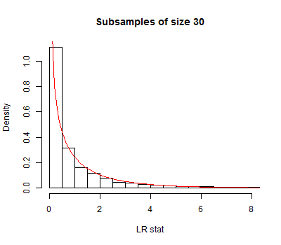
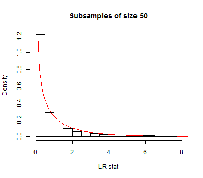
Figure 6: Histograms for the likelihood ratio test statistic for 5000 subsamples of size 30 and 50, respectively. The superimposed red line depicts the $\chi^{2}_{1}$ density.

For each subsample, we first fit the sub-model corresponding to the mixed graph depicted in Figure 5 without the edge PIP2 $\rightarrow$ PIP3. For this procedure, we initialize the free entries of $B$ using least squares regression estimates (i.e., fitting the model that ignores the error correlations). We then calculate the covariance between the regression residuals to estimate the non-zero elements of $\Omega$. Although the sample covariance of the regression residuals is positive definite, the resulting matrix which also encodes the structural zeros may not be. To ensure that $\Omega$ is positive definite, we scale the off diagonal elements such that $\sum_{i\neq j}|\omega_{ij}|=.9\times\omega_{ii}$ so that the resulting matrix is diagonally dominant. After the BCD algorithm converges to a stationary point in the sub-model, we take the fitted values $\hat{B}$ and $\hat{\Omega}$ to initialize the algorithm run on the model that includes the additional PIP2 $\rightarrow$ PIP3 edge. We evaluate the likelihood function at each of the two maxima and formulate the corresponding likelihood ratio test statistic. The choice of $\hat{B}$ and $\hat{\Omega}$ as initial values for estimating the larger model guarantees that the test statistics are non-negative.

Histograms for the subsampled log-likelihood ratio statistics are shown in Figure 6. The empirical distributions for $b=30$ and $b=50$ are seen to be similar to one another and also rather close to a $\chi^{2}_{1}$ distribution. The observed test statistic for the full data has empirical p-value of 0.76 and 0.73 for $b=30$ and $b=50$ respectively. These p-values are slightly smaller than the p-value of 0.78 from $\chi^{2}_{1}$ approximation. Altogether there is little evidence to reject the sub-model in favor of the more complicated cyclic model.

5.2 Simulated data

We now demonstrate how the BCD algorithm behaves on different types of mixed graphs. We consider the existing R package ‘sem’ (Fox, 2006) as an alternative and compare the performance of these algorithms for maximum likelihood estimation on simulated data.

To simulate a mixed graph, we begin with the empty graph on $V$ nodes. For $0\leq k\leq V$, we add directed edges $1\to 2\to\cdots\to(k-1)\to k\to 1$, creating a directed cycle of length $k$. For all $p(p-1)/2-(k-1)$ remaining pairs of nodes $(i,j)$ with $i<j$, we generate independent uniform random variables $U_{ij}\sim U(0,1)$. If $U_{ij}\leq d$, we introduce the directed edge $i\to j$. Alternatively, if $d<U_{ij}\leq b+d$, we introduce the bi-directed edge $i\leftrightarrow j$. If $U_{ij}>b+d$, there is no edge between $i$ and $j$. After all edges have been determined, we randomly permute the node labels. This construction ensures that the resulting mixed graph $G$ has the following properties:

1. $G$ has a unique cycle of length $k$;

2. $G$ is bow-free and simple.

For this simulation, we use 24 different configurations of $(V,N,k,d,b)$, where $N$ is the sample size. We examine graphs of size $V=10$ and $V=20$ and $N=3V/2$ and $N=10V$ observations. In each of these 4 configurations, we consider 3 distinct choices of the maximum cycle length: $k=0$, $V/5$, and $2V/5$. For each combination of $(V,N,k)$, we let $d=0.1$ and $d=0.2$, fixing $b=d/2$ in each case. Note that in the case of $k=0$, every generated graph will be acyclic and simple, the class of mixed graphs considered by Drton, Eichler and Richardson (2009).

				Convergence		Both	Both	Running time
$V$	$N$	$k$	$d$	BCD	SEM	converge	agree	BCD	SEM
10	15	0	0.1	1000	991	991	932	3.8	24.1
10	15	0	0.2	1000	949	949	884	9.5	31.8
10	15	2	0.1	1000	479	479	456	10.7	28.7
10	15	2	0.2	1000	559	559	518	16.0	36.2
10	15	4	0.1	997	672	672	637	10.7	30.5
10	15	4	0.2	997	553	553	520	16.7	38.0
10	100	0	0.1	1000	996	996	985	6.5	30.9
10	100	0	0.2	1000	991	991	991	20.9	53.3
10	100	2	0.1	1000	517	517	517	40.1	48.0
10	100	2	0.2	1000	635	635	635	51.5	58.9
10	100	4	0.1	999	726	726	725	33.4	50.2
10	100	4	0.2	998	688	688	688	46.3	63.0
20	30	0	0.1	1000	989	989	971	54.0	324.7
20	30	0	0.2	1000	921	921	881	166.7	550.5
20	30	4	0.1	999	836	836	824	77.3	319.5
20	30	4	0.2	998	731	731	701	197.0	652.6
20	30	8	0.1	1000	709	709	696	97.0	342.2
20	30	8	0.2	999	534	534	505	237.5	766.3
20	200	0	0.1	1000	998	998	993	119.8	330.1
20	200	0	0.2	1000	983	983	958	299.0	585.4
20	200	4	0.1	1000	847	847	829	199.5	356.8
20	200	4	0.2	999	806	806	773	359.6	712.3
20	200	8	0.1	999	765	765	755	257.6	409.8
20	200	8	0.2	1000	659	659	630	471.7	851.4

Table 1: Data simulated from a random distribution in a randomly generated mixed graph model is fit to the model using BCD and the quasi-Newton method invoked by ‘sem’. Each row summarizes 1000 simulations. ‘Both agree’ counts the cases with ML estimates equal up to small tolerance. Running time is average CPU time (in milliseconds) for the cases in which both algorithms converged and agreed.

In each simulation, we generate a random mixed graph $G$ according to the procedure above. We then select a random distribution from the corresponding normal model $\mathbf{N}(G)$ by taking the covariance matrix to be $\Sigma=(I-B)^{-1}\Omega(I-B)^{-T}$ for $B\in\mathbf{B}(G)$ and $\Omega\in\mathbf{\Omega}(G)$ selected as follows. We set all free, off-diagonal entries of $B$ and $\Omega$ to independent realizations from a $\mathcal{N}(0,1)$ distribution. The diagonal entries of $\Omega$ are chosen as one more than the sum of the absolute values of the entries in the corresponding row of $\Omega$ plus a random draw from a $\chi^{2}_{1}$ distribution. Hence, $\Omega$ is diagonally dominant and positive definite. The model $\mathbf{N}(G)$ is then fit to a sample of size $N$ that is generated from the selected distribution. We use the routine ‘sem’ and our BCD algorithm. The BCD algorithm isallowed to run for a maximum of 5000 iterations, at which point divergence was assumed. The BCD algorithm is initialized using the procedure described in Section 5.1. The ‘sem’ method is initialized by default using a modification of the procedure described by McDonald and Hartmann (1992).

Each row of Table 1 corresponds to 1000 simulations at a configuration of $(V,N,k,d,b)$. In particular, we record how often each algorithm converges. The columns ‘both converge’ and ‘both agree’ report the number of simulations for which both algorithms converged, and the number of these simulations for which the resulting estimates were equal up to a small tolerance. For the routine ‘sem’, which uses a generic ‘nlm’ Newton optimizer, it is not uncommon that convergence occurs but yields estimates that are not positive definite. In these cases, we consider the algorithm to have not converged.

The last two columns show the average CPU running times (in milliseconds) over simulations for which both methods converged and agreed. We caution that these times are not directly comparable, since ‘sem’ computes a number of other quantities of interest in addition to the maximum likelihood estimate. However, the BCD algorithm is up to 6 times faster than ‘sem’ in some instances. One potential reason is that when the graph is relatively sparse, many of the nodes may only require a single BCD update.

6 Discussion

This work gives is an extension of the RICF algorithm from Drton, Eichler and Richardson (2009) to cyclic models. The RICF algorithm and its BCD extension iteratively perform partial maximizations of the likelihood function via joint updates to the parameter matrices $B$ and $\Omega$. Each update problem admits a unique solution. Like its predecessor, the generalized algorithm is guaranteed to produce feasible positive definite covariance matrices after every iteration. Moreover, any accumulation point of the sequence of estimated covariance matrices is necessarily either a local maximum or a saddle point of the likelihood function.

Despite these desirable properties, the general scope of this algorithm to cyclic models is not without limitations. As with any iterative maximization procedure, there is no guarantee that convergence of the algorithm is to a global maximum, due to possible multi-modality of the likelihood function. In addition, for certain models the algorithm may be ill-defined, due to collinearity of the covariates and pseudo-covariates in our update step. However, we show that the models for which this occurs are non-identifiable. Moreover, we give necessary and sufficient graphical conditions for generically well defined updates, which were not previously known for the acyclic case.

In some of our simulated examples the BCD algorithm, which does not use any overall second-order information, needed many iterations to meet a convergence criterion. It is possible that in those cases a hybrid method that also consider quasi-Newton steps would converge more quickly. Nevertheless, our numerical experiments in Section 5.2 show that the BCD algorithm is competitive in terms of computation time with the generic optimization tools as used in the R package ‘sem’ all the while alleviating convergence problems.

Appendix A Proofs for claims in Section 2

A.1 Proof of Lemma 1

Lemma 1.

Let $B=(\beta_{ij})\in\mathbf{B}(G)$ for a mixed graph $G$. Then

$$\det{(I-B)}\ =\sum_{\sigma\in\mathbf{S}_{V}(G)}(-1)^{n(\sigma)}\prod_{i\in V(\sigma)}\beta_{\sigma(i),i}.$$

Proof.

By the Leibniz formula,

$$\det(I-B)\;=\;\sum_{\sigma\in\mathbf{S}_{V}}\text{sgn}(\sigma)\prod_{i\in V}(I-B)_{\sigma(i),i}\;=\;\sum_{\sigma\in\mathbf{S}_{V}(G)}\text{sgn}(\sigma)\prod_{i\in V}(I-B)_{\sigma(i),i}.$$ (A.1)

The second equality in (A.1) holds because for all $\sigma\notin\mathbf{S}_{V}(G)$ there exists an index $i$ with $\sigma(i)\not=i$ and $i\to\sigma(i)\not\in E_{\to}$, which implies that $(I-B)_{\sigma(i),i}=-B_{\sigma(i),i}=0$ for $B\in\mathbf{B}(G)$. For a permutation $\sigma\in\mathbf{S}_{V}(G)$, and a cycle $\gamma\in\mathcal{C}(\sigma)$, define $V(\gamma)\subseteq V$ to be the set of nodes contained in the cycle $\gamma$. We may then rewrite (A.1) as

$$\sum_{\sigma\in\mathbf{S}_{V}(G)}\text{sgn}(\sigma)\prod_{i\in V}(I-B)_{\sigma(i),i} =\sum_{\sigma\in\mathbf{S}_{V}(G)}\prod_{\gamma\in\mathcal{C}(\sigma)}\left(\text{sgn}(\gamma)\prod_{i\in V(\gamma)}(I-B)_{\sigma(i),i}\right)$$

$$=\sum_{\sigma\in\mathbf{S}_{V}(G)}\prod_{\gamma\in\mathcal{C}_{2}(\sigma)}\left(\text{sgn}(\gamma)(-1)^{V(\gamma)}\prod_{i\in V(\gamma)}\beta_{\sigma(i),i}\right)$$

$$=\sum_{\sigma\in\mathbf{S}_{V}(G)}(-1)^{n(\sigma)}\prod_{i\in V(\sigma)}\beta_{\sigma(i),i}.$$ (A.2)

The last equation (A.2) is obtained from the fact that $\text{sgn}(\gamma)(-1)^{V(\gamma)}=-1$ for every cycle $\gamma\in\mathcal{C}_{2}(\sigma)$. This follows from noting that the sign of every even-length cycle is -1 and the sign of every odd-length cycle is 1. ∎

A.2 Derivation of the likelihood equations

Recall that the likelihood function for normal structural equation models takes the form

$$\ell_{G,Y}(B,\Omega) =\frac{N}{2}\log\det\left[(I-B)^{T}\Omega^{-1}(I-B)\right]-\frac{N}{2}\text{tr}\left[(I-B)^{T}\Omega^{-1}(I-B)S\right]$$

$$=\frac{N}{2}\log\det\left[(I-B)^{T}(I-B)\right]-\frac{N}{2}\log\det(\Omega)-\frac{N}{2}\text{tr}\left[(I-B)^{T}\Omega^{-1}(I-B)S\right].$$

Furthermore, recall that $\beta$ and $\omega$ are the vectors of free parameters in $B$ and $\Omega$ respectively. These vectors satisfy $\text{vec}(B)=P\beta$ and $\text{vec}(\Omega)=Q\omega$.

The first derivatives of the log-likelihood function with respect to $\beta$ and $\omega$ are

$$\frac{\partial\ell_{G,Y}(B,\Omega)}{\partial\beta} =\frac{\partial P\beta}{\partial\beta}\times\frac{\partial\ell_{G,Y}(B,\Omega)}{\partial\text{vec}(B)}$$

$$=P^{T}\ \text{vec}\left(\frac{\partial\ell_{G,Y}(B,\Omega)}{\partial B}\right)$$

$$=-\frac{N}{2}P^{T}\ \text{vec}\left[2(I-B)^{-T}\right.$$

$$\qquad\qquad\qquad\left.+\frac{\partial}{\partial B}\text{tr}\left(\Omega^{-1}S-B^{T}\Omega^{-1}S-\Omega^{-1}BS+B^{T}\Omega^{-1}BS\right)\right]$$

$$=-\frac{N}{2}P^{T}\ \text{vec}\left[2(I-B)^{-T}-2\Omega^{-1}S+\frac{\partial}{\partial B}\text{tr}\left(BSB^{T}\Omega^{-1}\right)\right]$$

$$=-\frac{N}{2}P^{T}\ \text{vec}\left[2(I-B)^{-T}-2\Omega^{-1}(I-B)S\right]$$

$$=NP^{T}\ \text{vec}\left[\Omega^{-1}(I-B)S-(I-B)^{-T}\right],$$

$$\frac{\partial\ell_{G,Y}(B,\Omega)}{\partial\omega} =\frac{\partial Q\omega}{\partial\omega}\times\frac{\partial\ell_{G,Y}(B,\Omega)}{\partial\text{vec}(\Omega)}$$

$$=Q^{T}\ \text{vec}\left(\frac{\partial\ell_{G,Y}(B,\Omega)}{\partial\Omega}\right)$$

$$=-\frac{N}{2}Q^{T}\ \text{vec}\left[\Omega^{-1}-\Omega^{-1}(I-B)S(I-B)^{T}\Omega^{-1}\right].$$

∎

Appendix B Proofs of claims in Section 3

B.1 Proof of Lemma 4

Lemma 4.

In (3.9), the vector $c$ is orthogonal to the kernel of $X$.

Proof.

The kernel of $X$ is orthogonal to the span of $X^{T}$. Hence, we have to show that

$$c=\begin{pmatrix}0\\ c_{i,{\rm pa}(i)}\end{pmatrix}\;\in\;\operatorname{span}\left(\begin{pmatrix}Z_{{\rm sib}(i)}\\ Y_{{\rm pa}(i)}\end{pmatrix}\right).$$

To be clear, the $N$ columns of the displayed matrix span a subspace of $\mathbb{R}^{{\rm sib}(i)}\times\mathbb{R}^{{\rm pa}(i)}$. We will in fact show something stronger, namely,

$$c=\begin{pmatrix}0\\ c_{i,{\rm pa}(i)}\\ -c_{i,0}\end{pmatrix}\;\in\;\operatorname{span}\left(\begin{pmatrix}Z_{{\rm sib}(i)}\\ Y_{{\rm pa}(i)}\\ Y_{i}\end{pmatrix}\right).$$

For notational convenience, let

$$\Delta\;:=\;\Omega^{-1}_{-i,-i}(I-B)_{-i}.$$ (B.1)

Then

$$\begin{pmatrix}Z_{{\rm sib}(i)}\\ Y_{{\rm pa}(i)}\\ Y_{i}\end{pmatrix}=\begin{pmatrix}0&\Delta_{{\rm sib}(i),{\rm pa}(i)}&\Delta_{{\rm sib}(i),V\setminus({\rm pa}(i)\cup\{i\})}\\ 0&I_{{\rm pa}(i)}&0\\ 1&0&0\end{pmatrix}\begin{pmatrix}Y_{i}\\ Y_{{\rm pa}(i)}\\ Y_{V\setminus({\rm pa}(i)\cup\{i\})}\end{pmatrix}.$$

Since the data matrix $Y$ is assumed to have full rank, it suffices to show that there is a vector $w\in\mathbb{R}^{V}$ such that

$$\begin{pmatrix}0&\Delta_{{\rm sib}(i),{\rm pa}(i)}&\Delta_{{\rm sib}(i),V\setminus({\rm pa}(i)\cup\{i\})}\\ 0&I_{{\rm pa}(i)}&0\\ 1&0&0\end{pmatrix}w\;=\;\begin{pmatrix}0\\ c_{i,{\rm pa}(i)}\\ -c_{i,0}\end{pmatrix}.$$ (B.2)

Consider any node $p\in{\rm pa}(i)$. For a permutation $\sigma\in\mathbf{S}_{V}$, i.e., a permutation of the vertex set $V$, let $\gamma_{i}(\sigma)$ be the permutation cycle containing $i$. Then, from Lemma 1, the vector $c$ has the coordinate indexed by $p$ equal to

$$c_{p} \;=\;\sum_{\begin{subarray}{c}\sigma\in\textbf{S}_{V}(G)\\ \sigma:\sigma(p)=i\end{subarray}}(-1)^{n(\sigma)}\prod_{j\in V(\gamma_{i}(\sigma))\setminus\{p\}}\beta_{\sigma(j),j}\prod_{\gamma\in\mathcal{C}_{2}(\sigma)\setminus\{\gamma_{i}(\sigma)\}}\prod_{k\in V(\gamma)}\beta_{\sigma(k),k}\,.$$

Let $\Psi_{i}$ be the set of all directed cycles in the graph $G$ that contain node $i$. For later convenience, we also include in $\Psi_{i}$ a self-loop $i\to i$. If $\gamma\in\Psi_{i}$, then write $P^{\gamma}_{i:k}$ for the product of coefficients $\beta_{lj}$ for edges $j\to l$ that lie on the directed path from $i$ to $k$ that is part of cycle $\gamma$, with $P^{\gamma}_{i:i}=1$. We set $P^{\gamma}_{i:k}=0$ if $k\not\in\gamma$. Then

$$c_{p} \;=\;\sum_{\gamma\in\Psi_{i}}P^{\gamma}_{i:p}\left(\sum_{\begin{subarray}{c}\sigma\in\textbf{S}_{V}(G)\\ \sigma:\gamma\subseteq\sigma\end{subarray}}(-1)^{n(\sigma)}\prod_{\begin{subarray}{c}\gamma^{\prime}\in\mathcal{C}_{2}(\sigma)\\ \gamma^{\prime}\neq\gamma\end{subarray}}\prod_{j\in V(\gamma^{\prime})}\beta_{\sigma(j),j}\right)\;=:\;\sum_{\gamma\in\Psi_{i}}P^{\gamma}_{i:p}\xi_{\gamma}.$$ (B.3)

Similarly, we have

$$c_{i,0}\;=\;-\sum_{\begin{subarray}{c}\sigma\in\textbf{S}_{V}(G)\\ \sigma:\sigma(i)=i\end{subarray}}(-1)^{n(\sigma)}\prod_{\gamma\in\mathcal{C}_{2}(\sigma)\setminus\{(i)\}}\prod_{k\in V(\gamma)}\beta_{\sigma(k),k}\,.$$

The negative sign in front is due to the fact that in the matrix $I-B$ the off-diagonal entries are negated but the diagonal entries are not. Having included the self-loop $i\to i$ in $\Psi_{i}$, we obtain that

$$c_{i,0}\;=\;-\sum_{\gamma\in\Psi_{i}}P^{\gamma}_{i:i}\xi_{\gamma}\;=\;-\sum_{\gamma\in\Psi_{i}}\xi_{\gamma}.$$ (B.4)

Using the sums $\xi_{\gamma}$ from (B.3), define $w$ to be the vector with coordinates

$$w_{k}=\sum_{\gamma\in\Psi_{i}}P^{\gamma}_{i:k}\xi_{\gamma},\quad k\in V.$$ (B.5)

By (B.3) and (B.4), the vector $w$ satisfies the equations in (B.2) that are indexed by ${\rm pa}(i)\cup\{i\}$. We now show that it also satisfies those indexed by ${\rm sib}(i)$.

Let $k\in V\setminus\{i\}$. Since every directed path from $i$ to $k$ passes through one of the parents of $k$, we have

$$P^{\gamma}_{i:k}\;=\;\sum_{p\in{\rm pa}(k)}P^{\gamma}_{i:p}\beta_{kp}$$

for any cycle $\gamma\in\Psi_{i}$ that contains $k$. Therefore,

$$\left((I-B)_{-i}w\right)_{k}=w_{k}-\sum_{p\in{\rm pa}(k)}\beta_{kp}w_{p}=\sum_{\gamma\in\Psi_{i}}P^{\gamma}_{i:k}\xi_{\gamma}-\sum_{p\in{\rm pa}(k)}\beta_{kp}\sum_{\gamma\in\Psi_{i}}P^{\gamma}_{i:p}\xi_{\gamma}=0.$$

In other words, $w$ is in the kernel of $(I-B)_{-i}$. This kernel is contained in the kernel of $\Delta_{{\rm sib}}$, which yields (B.2). ∎

B.2 Proof of Lemma 5

Lemma 5.

For constants $a,b,c_{0},c_{1}\in\mathbb{R}$ with $c_{1}\neq 0$, define the function

$$f(x)=\frac{(a-x)^{2}+b^{2}}{(c_{0}+c_{1}x)^{2}},\qquad x\in\mathbb{R}\setminus\left\{-c_{0}/c_{1}\right\}.$$

1. If $c_{0}+ac_{1}\neq 0$, then $f$ is uniquely minimized by

   $$x=\frac{ac_{0}+a^{2}c_{1}+b^{2}c_{1}}{c_{0}+ac_{1}}=a+\frac{b^{2}c_{1}}{c_{0}+ac_{1}}.$$

2. If $c_{0}+ac_{1}=0$ and $b=0$, then $f$ is constant and equal to $1/c_{1}^{2}$.

3. If $c_{0}+ac_{1}=0$ and $b^{2}>0$, then $f$ does not achieve its minimum, and $\inf f=\lim_{x\to\pm\infty}f(x)=1/c_{1}^{2}$.

Proof.

The lemma is concerned with the univariate rational function

$$f(x)=\frac{(a-x)^{2}+b^{2}}{(c_{i,0}+c_{1}x)^{2}},\qquad x\in\mathbb{R},$$

where $a,b,c_{i,0},c_{1}\in\mathbb{R}$ are constants with $c_{1}\neq 0$. The function $f$ is defined everywhere except at the point $x=-c_{i,0}/c_{1}$. The limits of $f$ are

$$\lim_{x\to\infty}f(x)=\lim_{x\to-\infty}f(x)=\frac{1}{c_{1}^{2}}.$$ (B.6)

Note that

$$f^{\prime}(x)=-\frac{2(ac_{i,0}+a^{2}c_{1}+b^{2}c_{1}-c_{i,0}x-ac_{1}x)}{(c_{i,0}+c_{1}x)^{3}}.$$ (B.7)

Equating (B.7) to zero and solving results in one critical point:

$$x^{\star}=\frac{ac_{i,0}+a^{2}c_{1}+b^{2}c_{1}}{c_{i,0}+ac_{1}},$$ (B.8)

which is finite if $c_{i,0}+ac_{1}\neq 0$. Moreover, observe that

$$f(x^{\star})=\frac{b^{2}}{(c_{i,0}+ac_{1})^{2}+b^{2}c_{1}^{2}}<\frac{1}{c_{1}^{2}}.$$ (B.9)

The second derivative of $f$ is given by

$$f^{\prime\prime}(x)=\frac{2(c_{i,0}^{2}+4ac_{i,0}c_{1}+3a^{2}c_{1}^{2}+3b^{2}c_{1}^{2}-2c_{i,0}c_{1}x-2ac_{1}^{2}x)}{(c_{i,0}+c_{1}x)^{4}},$$

from which it is revealed that

$$f^{\prime\prime}(x^{\star})=\frac{2(c_{i,0}+ac_{1})^{4}}{\left((c_{i,0}+ac_{1})^{2}+b^{2}c_{1}^{2}\right)^{3}}>0.$$

Hence, we see that $x^{\star}$ in (B.8) is the unique critical point and is a local minimum. Moreover, from (B.6) and (B.9), we see that $x^{\star}$ must be the global minimum. If instead $c_{i,0}+ac_{1}=0$ and $b\not=0$, then (B.8) reveals that there are no critical points, and at the pole we have $\lim_{x\to-c_{i,0}/c_{1}}f(x)=\infty$. It thus follows that $f$ achieves its minimum at $x=\pm\infty$. The case of $c_{i,0}+ac_{1}=0$ and $b=0$ is clear. ∎

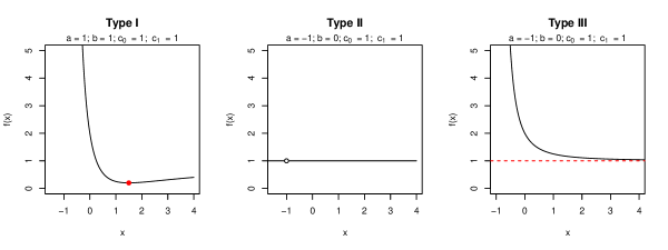
Figure 7: Examples of functions from the three cases in Lemma 5. A unique minimum is achieved only in Type I (indicated by the point).

B.3 Proof of claim in Remark 3

We use the notation from the proof of Lemma 4. Since $Y_{i}^{T}$ is in the span of $X$, we have $y_{0}^{2}=0$ and the least squares vector $\hat{\alpha}$ satisfies that

$$Y_{i}=e_{i}^{T}Y=\hat{\alpha}^{T}\begin{pmatrix}Z_{{\rm sib}(i)}\\ Y_{{\rm pa}(i)}\end{pmatrix}=\hat{\alpha}^{T}\begin{pmatrix}\Delta_{{\rm sib}(i),{\rm pa}(i)}&\Delta_{{\rm sib}(i),V\setminus{\rm pa}(i)}\\ I_{{\rm pa}(i)}&0\end{pmatrix}\begin{pmatrix}Y_{{\rm pa}(i)}\\ Y_{V\setminus{\rm pa}(i)}\end{pmatrix},$$

where $e_{i}$ is the $i$-th canonical basis vector. Since $Y$ has full rank, it follows that

$$e_{i}^{T}\;=\;\hat{\alpha}^{T}\begin{pmatrix}\Delta_{{\rm sib}(i),{\rm pa}(i)}&\Delta_{{\rm sib}(i),V\setminus{\rm pa}(i)}\\ I_{{\rm pa}(i)}&0\end{pmatrix}.$$

In the proof of Lemma 4, we constructed a vector $w\in\mathbb{R}^{V}$ such that

$$c=\begin{pmatrix}0\\ c_{i,{\rm pa}(i)}\\ -c_{i,0}\end{pmatrix}=\begin{pmatrix}0&\Delta_{{\rm sib}(i),{\rm pa}(i)}&\Delta_{{\rm sib}(i),V\setminus{\rm pa}(i)}\\ 0&I_{{\rm pa}(i)}&0\\ 1&0&0\end{pmatrix}w.$$

We find that

$$c^{T}\hat{\alpha}^{T}=\langle\begin{pmatrix}\Delta_{{\rm sib}(i),{\rm pa}(i)}&\Delta_{{\rm sib}(i),V\setminus{\rm pa}(i)}\\ I_{{\rm pa}(i)}&0\end{pmatrix}w,\hat{\alpha}\rangle=\langle w,e_{i}\rangle=w_{i}=-c_{i,0}.$$

Appendix C Proofs of claims in Section 4

C.1 Proof of Proposition 2

Proposition 2.

Let $G=(V,E_{\to},E_{\leftrightarrow})$ be a mixed graph, and let $i\in V$. Then the following two statements are equivalent:

1. Condition (A1)_i holds for generic triples $(Y,B,\Omega)\in\mathbb{R}^{V\times N}\times\mathbf{B}(G)\times\mathbf{\Omega}(G)$.

2. The induced subgraph $G_{-i}$ contains a system of half-collider paths from a subset of $V\setminus({\rm pa}(i)\cup\{i\})$ to ${\rm sib}(i)$ such that the bi-directed portions are pairwise disjoint.

Proof.

For notational convenience, let

$$\Lambda\;:=\;(I-B)_{-i}\qquad\text{and}\qquad\Delta\;:=\;\Omega^{-1}_{-i,-i}\Lambda=\Omega^{-1}_{-i,-i}(I-B)_{-i}.$$

Then

$$\begin{pmatrix}Z_{{\rm sib}(i)}\\ Y_{{\rm pa}(i)}\\ Y_{i}\end{pmatrix}=\begin{pmatrix}0&\Delta_{{\rm sib}(i),{\rm pa}(i)}&\Delta_{{\rm sib}(i),V\setminus({\rm pa}(i)\cup\{i\})}\\ 0&I_{{\rm pa}(i)}&0\\ 1&0&0\end{pmatrix}\begin{pmatrix}Y_{i}\\ Y_{{\rm pa}(i)}\\ Y_{V\setminus({\rm pa}(i)\cup\{i\})}\end{pmatrix}.$$ (C.1)

$(a)\Longrightarrow(b)$. If the matrix above has full row rank, then $rk\left(\Delta_{{\rm sib}(i),V\setminus\{{\rm pa}(i)\cup i\}}\right)=|{\rm sib}(i)|=S_{i}$. This implies that there exists a $S_{i}\times S_{i}$ submatrix of $\Delta_{{\rm sib}(i),V\setminus\left({\rm pa}(i)\cup\{i\}\right)}$ which has full rank. Let that full rank sub-matrix be $\Delta_{{\rm sib}(i),\tilde{V}}$ where $\tilde{V}\subseteq V\setminus\{{\rm pa}(i)\cup i\}$ where $|\tilde{V}|=S_{i}$. By the Cauchy-Binet formula, we have

$$\det\Delta_{{\rm sib}(i),\tilde{V}}=\sum_{A\in\left\{V\setminus i\atop S_{i}\right\}}\det\left[\Omega^{-1}_{-i,-i}\right]_{{\rm sib}(i),A}\det\Lambda_{A,\tilde{V}}.$$

Since $\det\Delta_{{\rm sib}(i),\tilde{V}}\neq 0$ by construction, there must exist a set $A\subseteq V\setminus\{i\}$ with $|A|=S_{i}$ for which both $\det[\Omega^{-1}_{-i,-i}]_{{\rm sib}(i),A}\neq 0$ and $\det\Lambda_{A,\tilde{V}}\neq 0$.

Let $D$ be a $\mathbb{R}^{V-1\times V-1}$ diagonal matrix with $\left(\sqrt{\omega_{11}},\ldots\sqrt{\omega_{i-1,i-1}},\sqrt{\omega_{i+1,i+1}}\ldots\sqrt{\omega_{VV}}\right)$ on the diagonal. Let $I-W$ be the correlation matrix corresponding to $\Omega_{-i,-i}$, so that $D(I-W)D=\Omega_{-i,-i}$ and $(I-W)^{-1}=D\Omega^{-1}_{-i,-i}D$. Then, $\det[\Omega^{-1}_{-i,-i}]_{{\rm sib}(i),A}\neq 0$ implies that

$$0 \neq\det D_{{\rm sib}(i),{\rm sib}(i)}\det[\Omega^{-1}_{-i,-i}]_{{\rm sib}(i),A}\det D_{A,A}$$

$$=\sum_{B,C\in{V\setminus i\choose S_{i}}}\det D_{{\rm sib}(i),B}\det[\Omega^{-1}_{-i,-i}]_{B,C}\det D_{C,A}$$

$$=\det\left[D\Omega^{-1}_{-i,-i}D\right]_{{\rm sib}(i),A}$$

$$=\det\left[(I-W)^{-1}\right]_{{\rm sib}(i),A},$$

where the first equality holds because $\det D_{J,K}\neq 0$ iff $J=K$ since $D$ is diagonal. Applying Corollary 3.8 from Sullivant, Talaska and Draisma (2010), we see that $\det\left[(I-W)^{-1}\right]_{{\rm sib}(i),A}\neq 0$ implies that there exists a system $\mathcal{P}$ of vertex disjoint bi-directed paths from ${\rm sib}(i)$ to $A$.

A Leibniz expansion of $\det\Lambda_{A,\tilde{V}}$ shows that $\det\Lambda_{A,\tilde{V}}\not=0$ implies that the graph contains a matching of $\tilde{V}$ and $A$. In other words, we can enumerate the sets as $\tilde{V}=\{v_{1},\dots,v_{S_{i}}\}$ and $A=\{a_{1},\dots,a_{S_{i}}\}$ such that $v_{s}=a_{s}$ or $v_{s}\in{\rm pa}(a_{s})$ for $s=1,\dots,S_{i}$. Since we have the system $\mathcal{P}$ of vertex disjoint bi-directed paths from ${\rm sib}(i)$ to $A$, there is thus a system of half-collider paths with pairwise disjoint bi-directed portions. The paths are fully contained in $\mathcal{G}_{-i}$ because we considered $\Omega_{-i,-i}$ and $\tilde{V}\subseteq V\setminus\left({\rm pa}(i)\cup\{i\}\right)$.

$(a)\Longleftarrow(b)$. When $Y$ is full rank (which is true for generic $Y$ when $N\geq|V|$), a drop in the row rank of the matrix displayed in (C.1) is equivalent to a drop in rank of $\Delta_{{\rm sib}(i),V\setminus\left({\rm pa}(i)\cup\{i\}\right)}$. We show that given a set of nodes $\tilde{V}$ that satisfies the assumed graphical condition, the matrix $\Delta_{{\rm sib}(i),V\setminus\left({\rm pa}(i)\cup\{i\}\right)}$ is generically of full rank since there is an $S_{i}\times S_{i}$ minor which only vanishes on a set of pairs $(B,\Omega)$ with Lebesgue measure 0. Here, $|\tilde{V}|=|{\rm sib}(i)|=S_{i}$. In what follows we consider systems of half-collider paths from $\tilde{V}$ to ${\rm sib}(i)$. We always index the paths as $\pi^{s}$ where $s$ is the endpoint in ${\rm sib}(i)$. We write $v_{s}$ for the other endpoint of $\pi^{s}$, so $v_{s}\in\tilde{V}$.

First, given a valid half-collider path system $\mathcal{P}=\{\pi^{s}\}_{s\in{\rm sib}(i)}$, we claim that there exists an ordering $\prec$ of ${\rm sib}(i)$ and a system of half-collider paths $\mathcal{\hat{P}}=\{\hat{\pi}^{s}\}_{s\in{\rm sib}(i)}$ such that $r\prec s$ implies that the first node of $\hat{\pi}^{s}$ is not in the bi-directed portion of $\hat{\pi}^{r}$. Note that if the first node of a half-collider path is the tail of a directed edge, it can still appear in the bi-directed portion of another path in a valid path system. Suppose that the specified ordering does not exist. Then there is a set of nodes $G_{\text{cycle}}=\{g_{1},g_{2}\dots g_{q}\}\subseteq{\rm sib}(i)$ where the first node of $\pi^{g_{k}}$ is in the bi-directed portion of $\pi^{g_{k-1}}$ for $k>1$ and the first node of $\pi^{g_{1}}$ is in the bi-directed portion of $\pi^{g_{q}}$. Then this implies that for each $g_{i}\in G_{\text{cycle}}$, there exists some node in the half-collider path $\pi^{g_{i}}$ closer to $g_{i}$ which is not in ${\rm pa}(i)$, namely the first node of $\pi^{g-1}$. Thus, simply removing the first directed edge of each of the half-collider paths produces a valid system $\mathcal{\hat{P}}$ that can be ordered as claimed. For the remainder of the proof, we assume without loss of generality that the considered system of half-collider paths $\mathcal{P}$ has the desired ordering.

Consider the $S_{i}\times S_{i}$ sub-matrix $\Delta_{{\rm sib}(i),\tilde{V}}$, and note that the determinant of $\Delta_{{\rm sib}(i),\tilde{V}}$ is a rational function of the elements of $\Omega$ and $B$. To show that both the numerator and denominator only vanish on a null set, we appeal to Lemma 1 from Okamoto (1973) which states that the zero set of a nonzero polynomial is a null set. To show that the numerator and denominator are not 0 everywhere, consider the point $\left(\Omega^{\dagger},B^{\dagger}\right)$ whose coordinates are specified as follows:

• Set all diagonal entries $\omega_{kk}^{\dagger}$ to 1;

• Set $\omega_{jk}^{\dagger}>0$ (but sufficiently small so that $\Omega$ is positive definite) if and only if $j\leftrightarrow k\in\pi^{s}$ for some $s\in{\rm sib}(i)$;

• Set $\beta_{kv_{s}}^{\dagger}=-1$ if and only if $k\leftarrow v_{s}\in\pi_{s}$;

• Set all other parameters to 0.

Note that the support of $\left(\Omega^{\dagger},B^{\dagger}\right)$ matches the edges of the half-collider paths in $\mathcal{P}$. Let $\delta^{\dagger}_{jk}$ and $\lambda^{\dagger}_{jk}$ be the entries of the matrices $\Delta_{{\rm sib}(i),\tilde{V}}$ and $\Lambda$ constructed from $\left(\Omega^{\dagger},B^{\dagger}\right)$. Let $\omega^{\star}_{jk}$ be the entries of $(\Omega^{\dagger}_{-i,-i})^{-1}$. Then

$$0\neq\tilde{\delta}^{\dagger}_{sv_{s}}=\sum_{k\in V\setminus i}\omega^{\star}_{sk}\lambda^{\dagger}_{kv_{s}}=\begin{cases}\omega^{\star}_{ss}&\mbox{ if }v_{s}=s,\\ \omega^{\star}_{sm}&\mbox{ if the first edge in $\pi^{s}$ is $v_{s}\rightarrow m$},\\ \omega^{\star}_{sv_{s}}&\mbox{ if the first edge in $\pi^{s}$ is bi-directed}.\end{cases}$$

For any $r\neq s$,

$$\delta^{\dagger}_{sv_{r}}=\sum_{k\in V\setminus i}\omega^{\star}_{sk}\lambda^{\dagger}_{kv_{s}}=\begin{cases}\omega^{\star}_{sa_{r}}&\mbox{ if the first node of $\pi^{r}$ is in $\pi^{s}$},\\ 0&\mbox{ else}.\end{cases}$$

By the assumed ordering of ${\rm sib}(i)$, if the first node of $\pi_{r}$ lies on $\pi_{s}$ then $s\succ r$. Therefore, there is a permutation of the rows and columns of $\Delta_{{\rm sib}(i),\tilde{V}}$ that makes the matrix upper triangular with $\delta^{\dagger}_{s\hat{v}_{s}}$ on the diagonal. Hence, the determinant is

$$\det\Delta^{\dagger}_{{\rm sib}(i),\tilde{V}}=\prod_{s}\tilde{\delta}^{\dagger}_{s\hat{v}_{s}}\neq 0.$$

It follows that the determinant of $\Delta_{{\rm sib}(i),\tilde{V}}$ is nonzero almost everywhere. The assumed graphical condition thus implies that the matrix in (C.1) has generically full rank. ∎

C.2 Proof of Theorem 3

Theorem 3.

For a mixed graph $G=(V,E_{\to},E_{\leftrightarrow})$, the following two statements are equivalent:

1. For all $i\in V$, the induced subgraph $G_{-i}$ contains a system of half-collider paths from a subset of $V\setminus({\rm pa}(i)\cup\{i\})$ to ${\rm sib}(i)$ such that the bi-directed portions are pairwise disjoint.

2. For generic triples $(Y,B_{0},\Omega_{0})\in\mathbb{R}^{V\times N}\times\mathbf{B}(G)\times\mathbf{\Omega}(G)$, any finite number of iterations of the BCD algorithm for $\ell_{G,Y}$ have unique and feasible block updates when $(B_{0},\Omega_{0})$ is used as starting value.

Proof.

If the graphical condition (a) fails then, by Proposition 2 and Theorem 2, there exists a node $i\in V$ at which the BCD algorithm does not have a unique and feasible update, irrespective of the choice of $(Y,B_{0},\Omega_{0})$.

Conversely, suppose condition (a) holds. Let $i(t)$ be the node considered in step $t$ of the BCD algorithm, and let $(B_{t},\Omega_{t})$ be the pair of parameter matrices after the $t$-th block update. By Theorem 2, each pair $(B_{t},\Omega_{t})$ is a rational function of the input triple $(Y,B_{t-1},\Omega_{t-1})$. For $i=i(t)$, the conditions (A1)_i and (A2)_i from Proposition 2 are rational conditions on $(Y,B_{t-1},\Omega_{t-1})$. Therefore, for any $T\geq 1$ there is a rational function $f_{T}(Y,B,\Omega)$ such that $f_{T}(Y,B_{0},\Omega_{0})\not=0$ if and only if the BCD updates at $i(1),\dots,i(T)$ all have unique feasible solutions. By Okamoto (1973, Lemma 1), it now suffices to show that there exists a triple $(Y,B_{0},\Omega_{0})$ such that when started at $(B_{0},\Omega_{0})$ the BCD updates at $i(t)$, $t\leq T$, all have unique and feasible solutions.

When condition (a) holds and $Y$ is full rank, (A1)_i holds for generic $\Omega$ and $B$ for all $i\in V$. Thus, we may pick $\Omega_{0}$ and $B_{0}$ such that (A1)_i holds for every $i\in V$. Now choose $Y$ as in the proof of Proposition 3, with $(I-B_{0})^{-1}\Omega_{0}(I-B_{0})^{-T}=\frac{1}{N}YY^{T}$. Then as shown when proving Proposition 3, condition (A2)_i holds for every $i\in V$. By Proposition 2, the first BCD update problem has a unique feasible solution. This solution is $(B_{1},\Omega_{1})=(B_{0},\Omega_{0})$ because $(B_{0},\Omega_{0})$ is a global maximizer of the likelihood function by definition of $Y$. By induction, we have $(B_{t},\Omega_{t})=(B_{0},\Omega_{0})$ at all steps $t$. Consequently, for the triple $(Y,B_{0},\Omega_{0})$, any finite number of BCD updates have unique and feasible solutions, as we needed to show. ∎

C.3 Verifying graphical condition in polynomial time

Proposition 5.

For any mixed graph $G=(V,E_{\to},E_{\leftrightarrow})$, condition (a) in Theorem 3 can be checked in $\mathcal{O}(|V|^{5})$ operations.

Proof.

In order to show that condition (a) from Theorem 3 can be checked in $\mathcal{O}(|V|^{5})$ operations, it suffices to show that the condition imposed at each node $i\in V$ can be checked in $\mathcal{O}(|V|^{4})$ operations. So fix an arbitrary node $i\in V$.

If ${\rm pa}(i)\bigcap{\rm sib}(i)=\emptyset$, the condition is trivially satisfied by taking the set $\tilde{V}={\rm sib}(i)$. If ${\rm pa}(i)\bigcap{\rm sib}(i)\not=\emptyset$ (i.e., $j\rightarrow i\in E_{\rightarrow}$ and $j\leftrightarrow i\in E_{\leftrightarrow}$ for some $j\in V$), we can check the condition by considering a relevant flow network $\hat{G}_{i}$ which captures all half-collider paths to ${\rm sib}(i)$. In this network, we include a sink node connected to each node in ${\rm sib}(i)$ and a source node connected to each “allowable” node, that is, any node $j\not\in{\rm pa}(i)$ that can reach ${\rm sib}(i)$ through a half-collider path. In this network $\hat{G}_{i}$, the half-collider path criterion of Theorem 3 is satisfied if and only if the maximum flow from the source to the sink is equal to $|{\rm sib}(i)|$.

More specifically, the flow network $\hat{G}_{i}$ is constructed as follows:

1. Include a source $q$ and a sink $t$.

2. Let $C\subseteq V\setminus\{i\}$ be the set of all nodes with a bi-directed path to $i$ in ${G}$.

   1. Add a node $b(j)$ to $\hat{G}_{i}$ for each $j\in C$.

   2. For all $j,k\in C$ with $j\leftrightarrow k\in E_{\leftrightarrow}$, add edges $b(j)\rightarrow b(k)$ and $b(k)\rightarrow b(j)$ to $\hat{G}_{i}$.

   3. For each $j\in C\setminus{\rm pa}(i)$, if $j\in{\rm pa}(C)$, then include node $q(j)$ and add edges $q\rightarrow q(j)\rightarrow b(j)$ to $\hat{G}_{i}$. If $j\not\in{\rm pa}(C)$, then add edge $q\rightarrow b(j)$ to $\hat{G}_{i}$.

   4. For each $j\in{\rm pa}(C)\setminus\left({\rm pa}(i)\cup\{i\}\right)$, add node $d(j)$ and edges $d(j)\rightarrow b(m)$ for all $m\in C$ with $j\in{\rm pa}(m)$. If $j\in C$ then add edge $q(j)\rightarrow d(j)$, and if $j\not\in C$, add edge $q\rightarrow d(j)$.

   5. For each $j\in{\rm sib}(i)\cap C$, add edge $b(j)\rightarrow t$.

3. Let the capacity of $q$ and $t$ be $|{\rm sib}(i)|$. Let all other node capacities be 1. Set all edge capacities to 1.

The network $\hat{G}_{i}$ includes a directed path from source $q$ to sink $t$ to represent each valid half-collider path from $V\setminus\left({\rm pa}(i)\cup\{i\}\right)$ to $s\in{\rm sib}(i)$. In doing so, it is important to keep track of whether a nodes is in the bi-directed part of one half-collider path and the directed part of another half-collider path. To capture the directed and bi-directed roles of a node, respectively, we represent any node $j\in C\cap{\rm pa}(C)\setminus\left({\rm pa}(i)\cup\{i\}\right)$ with the two nodes $d(j)$ and $b(j)$ in $\hat{G}_{i}$. However, in order to ensure that each node $j$ is the beginning node for only one half-collider path in the path system (so that $\tilde{V}$ has cardinality $|{\rm sib}(i)|$), a bottleneck node $q(j)$ is included to ensure that at most 1 total unit of flow “originates” at the representations of $j$.

As shown in Lemma 6 below, the graphical condition can be checked by solving the maximum flow problem for $\hat{G}_{i}$. The standard max flow problem (with edge capacities but not node capacities) can be solved in $\mathcal{O}(|\hat{V}|^{2}|\hat{E}|)$, where $\hat{V}$ and $\hat{E}$ are the vertex and edge set of the network, respectively; see Edmonds and Karp (1970). To encode the node capacity constraints, we augment our network so that each node has an additional in/out node with a single edge pointing to/from the original node with the original node capacity. In the constructed network $|\hat{V}|\leq 5|V|$ and $|\hat{E}|\leq|\hat{V}|^{2}$ so the max flow problem for each individual node is $\mathcal{O}(|V|^{4})$, as was our claim. ∎

Lemma 6.

In the given mixed graph $G$, there exists a set of $|{\rm sib}(i)|$ nodes $\tilde{V}\subseteq V\setminus({\rm pa}(i)\cup\{i\})$ such that there is a system of half-collider paths $\mathcal{P}$ from $\tilde{V}$ to ${\rm sib}(i)$ where the bi-directed components are vertex distinct and do not include $i$, if and only if the constructed network $\hat{G}_{i}$ has maximum flow from source $q$ to sink $t$ of $|{\rm sib}(i)|$.

Proof.

Suppose there exists a system of half-collider paths $\mathcal{P}$ that satisfies the given condition. Then there is a corresponding system of paths from source $q$ to source $t$ in $\hat{G}_{i}$ with flow 1 over each edge. Since the bi-directed components are vertex distinct and each node in $\tilde{V}$ is distinct, we do not use any of the nodes in $\hat{G}_{i}$ more than once so none of the node or edge capacities are exceeded. Since there are $|{\rm sib}(i)|$ half-collider paths, the total flow is also $|{\rm sib}(i)|$.

Conversely, suppose the maximum flow on $\hat{G}_{i}$ is $|{\rm sib}(i)|$. Because each capacity is integer valued, the flow can be decomposed into a system $\mathcal{P}$ of directed paths with integer flow (Fulkerson, 1962). By construction, each path in $\mathcal{P}$ is a valid half-collider path which begins at some node $j\not\in\left({\rm pa}(i)\cup\{i\}\right)$ and ends at some $s\in{\rm sib}(i)$. In addition, since $q(j)$ only has capacity 1, the edges $q(j)\rightarrow d(j)$ and $q(j)\rightarrow b(j)$ cannot simultaneously be utilized in $\mathcal{P}$. Thus, each edge which carries flow from the source $q$ represents a distinct node in $V\setminus\left({\rm pa}(i)\cup\{i\}\right)$ and $|\tilde{V}|=|{\rm sib}(i)|$. Because there are only $|{\rm sib}(i)|$ edges to the sink, each connected to some node representing $s\in{\rm sib}(i)$, there is a half-collider path to each $s\in{\rm sib}(i)$. Finally, since the capacity of each node in $\hat{G}_{i}$ is one, each node $b(j)$ only appears once in the system which makes the bi-directed portions vertex distinct. ∎

References

- Anderson (2003) {bbook}[author] \bauthor\bsnmAnderson, \bfnmT. W.\binitsT. W. (\byear2003). \btitleAn introduction to multivariate statistical analysis, \beditionthird ed. \bseriesWiley Series in Probability and Statistics. \bpublisherWiley-Interscience [John Wiley & Sons], Hoboken, NJ. \bmrnumber1990662 \endbibitem
- Bollen (1989) {bbook}[author] \bauthor\bsnmBollen, \bfnmKenneth A.\binitsK. A. (\byear1989). \btitleStructural equations with latent variables. \bseriesWiley Series in Probability and Mathematical Statistics: Applied Probability and Statistics. \bpublisherJohn Wiley & Sons Inc., \baddressNew York. \bnoteA Wiley-Interscience Publication. \bmrnumberMR996025 (90k:62001) \endbibitem
- Chaudhuri, Drton and Richardson (2007) {barticle}[author] \bauthor\bsnmChaudhuri, \bfnmSanjay\binitsS., \bauthor\bsnmDrton, \bfnmMathias\binitsM. and \bauthor\bsnmRichardson, \bfnmThomas S\binitsT. S. (\byear2007). \btitleEstimation of a covariance matrix with zeros. \bjournalBiometrika \bvolume94 \bpages199–216. \endbibitem
- Colombo et al. (2012) {barticle}[author] \bauthor\bsnmColombo, \bfnmDiego\binitsD., \bauthor\bsnmMaathuis, \bfnmMarloes H.\binitsM. H., \bauthor\bsnmKalisch, \bfnmMarkus\binitsM. and \bauthor\bsnmRichardson, \bfnmThomas S.\binitsT. S. (\byear2012). \btitleLearning high-dimensional directed acyclic graphs with latent and selection variables. \bjournalAnn. Statist. \bvolume40 \bpages294–321. \endbibitem
- Drton (2009) {barticle}[author] \bauthor\bsnmDrton, \bfnmMathias\binitsM. (\byear2009). \btitleLikelihood ratio tests and singularities. \bjournalAnn. Statist. \bvolume37 \bpages979–1012. \endbibitem
- Drton, Eichler and Richardson (2009) {barticle}[author] \bauthor\bsnmDrton, \bfnmMathias\binitsM., \bauthor\bsnmEichler, \bfnmMichael\binitsM. and \bauthor\bsnmRichardson, \bfnmThomas S.\binitsT. S. (\byear2009). \btitleComputing maximum likelihood estimates in recursive linear models with correlated errors. \bjournalJ. Mach. Learn. Res. \bvolume10 \bpages2329–2348. \bmrnumber2563984 (2012d:62211) \endbibitem
- Drton and Maathuis (2017) {barticle}[author] \bauthor\bsnmDrton, \bfnmMathias\binitsM. and \bauthor\bsnmMaathuis, \bfnmMarloes\binitsM. (\byear2017). \btitleStructure learning in graphical modeling. \bjournalAnnual Review of Statistics and Its Application. \bnotein press. \endbibitem
- Drton and Richardson (2004) {barticle}[author] \bauthor\bsnmDrton, \bfnmMathias\binitsM. and \bauthor\bsnmRichardson, \bfnmThomas S\binitsT. S. (\byear2004). \btitleMultimodality of the likelihood in the bivariate seemingly unrelated regressions model. \bjournalBiometrika \bvolume91 \bpages383–392. \endbibitem
- Drton, Sturmfels and Sullivant (2009) {bbook}[author] \bauthor\bsnmDrton, \bfnmMathias\binitsM., \bauthor\bsnmSturmfels, \bfnmBernd\binitsB. and \bauthor\bsnmSullivant, \bfnmSeth\binitsS. (\byear2009). \btitleLectures on algebraic statistics. \bseriesOberwolfach Seminars \bvolume39. \bpublisherBirkhäuser Verlag, \baddressBasel. \bdoi10.1007/978-3-7643-8905-5 \bmrnumber2723140 (2012d:62004) \endbibitem
- Edmonds and Karp (1970) {bincollection}[author] \bauthor\bsnmEdmonds, \bfnmJack\binitsJ. and \bauthor\bsnmKarp, \bfnmRichard M.\binitsR. M. (\byear1970). \btitleTheoretical improvements in algorithmic efficiency for network flow problems. In \bbooktitleCombinatorial Structures and their Applications (Proc. Calgary Internat. Conf., Calgary, Alta., 1969) \bpages93–96. \bpublisherGordon and Breach, New York. \bmrnumber0266680 \endbibitem
- Fox (2006) {barticle}[author] \bauthor\bsnmFox, \bfnmJohn\binitsJ. (\byear2006). \btitleTeacher’s corner: Structural equation modeling with the sem package in R. \bjournalStructural equation modeling \bvolume13 \bpages465–486. \endbibitem
- Fox (2014) {bphdthesis}[author] \bauthor\bsnmFox, \bfnmChristopher\binitsC. (\byear2014). \btitleInterpretation and inference of linear structural equation models \btypePhD thesis, \bpublisherUniversity of Chicago. \endbibitem
- Foygel, Draisma and Drton (2012) {barticle}[author] \bauthor\bsnmFoygel, \bfnmRina\binitsR., \bauthor\bsnmDraisma, \bfnmJan\binitsJ. and \bauthor\bsnmDrton, \bfnmMathias\binitsM. (\byear2012). \btitleHalf-trek criterion for generic identifiability of linear structural equation models. \bjournalAnn. Statist. \bvolume40 \bpages1682–1713. \endbibitem
- Fulkerson (1962) {bbook}[author] \bauthor\bsnmFulkerson, \bfnmDelbert Ray\binitsD. R. (\byear1962). \btitleFlows in networks. \bpublisherPrinceton University Press. \endbibitem
- Grace et al. (2016) {barticle}[author] \bauthor\bsnmGrace, \bfnmJames B.\binitsJ. B., \bauthor\bsnmAnderson, \bfnmT. Michael\binitsT. M., \bauthor\bsnmSeabloom, \bfnmEric W.\binitsE. W., \bauthor\bsnmBorer, \bfnmElizabeth T.\binitsE. T., \bauthor\bsnmAdler, \bfnmPeter B.\binitsP. B., \bauthor\bsnmHarpole, \bfnmW. Stanley\binitsW. S., \bauthor\bsnmHautier, \bfnmYann\binitsY., \bauthor\bsnmHillebrand, \bfnmHelmut\binitsH., \bauthor\bsnmLind, \bfnmEric M.\binitsE. M., \bauthor\bsnmPärtel, \bfnmMeelis\binitsM., \bauthor\bsnmBakker, \bfnmJonathan D.\binitsJ. D., \bauthor\bsnmBuckley, \bfnmYvonne M.\binitsY. M., \bauthor\bsnmCrawley, \bfnmMichael J.\binitsM. J., \bauthor\bsnmDamschen, \bfnmEllen I.\binitsE. I., \bauthor\bsnmDavies, \bfnmKendi F.\binitsK. F., \bauthor\bsnmFay, \bfnmPhilip A.\binitsP. A., \bauthor\bsnmFirn, \bfnmJennifer\binitsJ., \bauthor\bsnmGruner, \bfnmDaniel S.\binitsD. S., \bauthor\bsnmHector, \bfnmAndy\binitsA., \bauthor\bsnmKnops, \bfnmJohannes M. H.\binitsJ. M. H., \bauthor\bsnmMacDougall, \bfnmAndrew S.\binitsA. S., \bauthor\bsnmMelbourne, \bfnmBrett A.\binitsB. A., \bauthor\bsnmMorgan, \bfnmJohn W.\binitsJ. W., \bauthor\bsnmOrrock, \bfnmJohn L.\binitsJ. L., \bauthor\bsnmProber, \bfnmSuzanne M.\binitsS. M. and \bauthor\bsnmSmith, \bfnmMelinda D.\binitsM. D. (\byear2016). \btitleIntegrative modelling reveals mechanisms linking productivity and plant species richness. \bjournalNature \bvolume529 \bpages390–393. \endbibitem
- Harary (1962) {barticle}[author] \bauthor\bsnmHarary, \bfnmFrank\binitsF. (\byear1962). \btitleThe determinant of the adjacency matrix of a graph. \bjournalSIAM Rev. \bvolume4 \bpages202–210. \bmrnumber0144330 \endbibitem
- Hoyle (2012) {bbook}[author] \beditor\bsnmHoyle, \bfnmRick H.\binitsR. H., ed. (\byear2012). \btitleHandbook of structural equation modeling. \bpublisherGuilford Press, \baddressNew York. \endbibitem
- Kline (2015) {bbook}[author] \bauthor\bsnmKline, \bfnmRex B.\binitsR. B. (\byear2015). \btitlePrinciples and practice of structural equation modeling, \bedition4th ed. \bpublisherGuilford Press, \baddressNew York. \endbibitem
- Lacerda et al. (2008) {binproceedings}[author] \bauthor\bsnmLacerda, \bfnmGustavo\binitsG., \bauthor\bsnmSpirtes, \bfnmPeter\binitsP., \bauthor\bsnmRamsey, \bfnmJoseph\binitsJ. and \bauthor\bsnmHoyer, \bfnmPatrik\binitsP. (\byear2008). \btitleDiscovering cyclic causal models by independent components analysis. In \bbooktitleProceedings of the Twenty-Fourth Conference Annual Conference on Uncertainty in Artificial Intelligence (UAI-08) \bpages366–374. \bpublisherAUAI Press, \baddressCorvallis, Oregon. \endbibitem
- Lauritzen (1996) {bbook}[author] \bauthor\bsnmLauritzen, \bfnmSteffen L.\binitsS. L. (\byear1996). \btitleGraphical models. \bpublisherOxford University Press. \endbibitem
- McDonald and Hartmann (1992) {barticle}[author] \bauthor\bsnmMcDonald, \bfnmRoderick P\binitsR. P. and \bauthor\bsnmHartmann, \bfnmWolfgang M\binitsW. M. (\byear1992). \btitleA procedure for obtaining initial values of parameters in the RAM model. \bjournalMultivariate Behavioral Research \bvolume27 \bpages57–76. \endbibitem
- Mooij and Heskes (2013) {binproceedings}[author] \bauthor\bsnmMooij, \bfnmJoris M.\binitsJ. M. and \bauthor\bsnmHeskes, \bfnmTom\binitsT. (\byear2013). \btitleCyclic causal discovery from continuous equilibrium data. In \bbooktitleProceedings of the 29th Annual Conference on Uncertainty in Artificial Intelligence (UAI-13) (\beditor\bfnmAnn\binitsA. \bsnmNicholson and \beditor\bfnmPadhraic\binitsP. \bsnmSmyth, eds.) \bpages431–439. \bpublisherAUAI Press. \endbibitem
- Narayanan (2012) {barticle}[author] \bauthor\bsnmNarayanan, \bfnmA.\binitsA. (\byear2012). \btitleA review of eight software packages for structural equation modeling. \bjournalThe American Statistician \bvolume66 \bpages129-138. \endbibitem
- Nowzohour, Maathuis and Bühlmann (2015) {barticle}[author] \bauthor\bsnmNowzohour, \bfnmChristopher\binitsC., \bauthor\bsnmMaathuis, \bfnmMarloes\binitsM. and \bauthor\bsnmBühlmann, \bfnmPeter\binitsP. (\byear2015). \btitleStructure learning with bow-free acyclic path diagrams. \bjournalArXiv e-prints. \endbibitem
- Okamoto (1973) {barticle}[author] \bauthor\bsnmOkamoto, \bfnmMasashi\binitsM. (\byear1973). \btitleDistinctness of the eigenvalues of a quadratic form in a multivariate sample. \bjournalAnn. Statist. \bvolume1 \bpages763–765. \bmrnumberMR0331643 (48 ##9975) \endbibitem
- Park and Raskutti (2016) {barticle}[author] \bauthor\bsnmPark, \bfnmGunwoong\binitsG. and \bauthor\bsnmRaskutti, \bfnmGarvesh\binitsG. (\byear2016). \btitleIdentifiability assumptions and algorithm for directed graphical models with feedback. \bjournalArXiv e-prints. \endbibitem
- Pearl (2009) {bbook}[author] \bauthor\bsnmPearl, \bfnmJudea\binitsJ. (\byear2009). \btitleCausality, \beditionSecond ed. \bpublisherCambridge University Press, \baddressCambridge. \bnoteModels, reasoning, and inference. \bmrnumber2548166 (2010i:68148) \endbibitem
- Politis, Romano and Wolf (1999) {bbook}[author] \bauthor\bsnmPolitis, \bfnmDimitris N.\binitsD. N., \bauthor\bsnmRomano, \bfnmJoseph P.\binitsJ. P. and \bauthor\bsnmWolf, \bfnmMichael\binitsM. (\byear1999). \btitleSubsampling. \bpublisherSpringer, New York. \endbibitem
- Richardson (1996) {binproceedings}[author] \bauthor\bsnmRichardson, \bfnmThomas\binitsT. (\byear1996). \btitleA discovery algorithm for directed cyclic graphs. In \bbooktitleProceedings of the Twelfth Conference Annual Conference on Uncertainty in Artificial Intelligence (UAI-96) \bpages454–461. \bpublisherMorgan Kaufmann, \baddressSan Francisco, CA. \endbibitem
- Richardson (1997) {barticle}[author] \bauthor\bsnmRichardson, \bfnmT. S.\binitsT. S. (\byear1997). \btitleA characterization of Markov equivalence for directed cyclic graphs. \bjournalInternational Journal of Approximate Reasoning \bvolume17 \bpages107–162. \endbibitem
- Rosseel (2012) {barticle}[author] \bauthor\bsnmRosseel, \bfnmYves\binitsY. (\byear2012). \btitlelavaan: An R package for structural equation modeling. \bjournalJournal of Statistical Software \bvolume48 \bpages1–36. \bdoi10.18637/jss.v048.i02 \endbibitem
- Sachs et al. (2005) {barticle}[author] \bauthor\bsnmSachs, \bfnmKaren\binitsK., \bauthor\bsnmPerez, \bfnmOmar\binitsO., \bauthor\bsnmPe’er, \bfnmDana\binitsD., \bauthor\bsnmLauffenburger, \bfnmDouglas A\binitsD. A. and \bauthor\bsnmNolan, \bfnmGarry P\binitsG. P. (\byear2005). \btitleCausal protein-signaling networks derived from multiparameter single-cell data. \bjournalScience \bvolume308 \bpages523–529. \endbibitem
- Silva (2013) {bincollection}[author] \bauthor\bsnmSilva, \bfnmRicardo\binitsR. (\byear2013). \btitleA MCMC approach for learning the structure of Gaussian acyclic directed mixed graphs. In \bbooktitleStatistical Models for Data Analysis (\beditor\bfnmPaolo\binitsP. \bsnmGiudici, \beditor\bfnmSalvatore\binitsS. \bsnmIngrassia and \beditor\bfnmMaurizio\binitsM. \bsnmVichi, eds.) \bpages343–351. \bpublisherSpringer. \endbibitem
- Spirtes (1995) {binproceedings}[author] \bauthor\bsnmSpirtes, \bfnmP.\binitsP. (\byear1995). \btitleDirected cyclic graphical representations of feedback models. In \bbooktitleUncertainty in Artificial Intelligence: Proceedings of the Conference (\beditor\bfnmP.\binitsP. \bsnmBesnard and \beditor\bfnmS.\binitsS. \bsnmHanks, eds.) \bpages491–498. \bpublisherMorgan Kaufmann, \baddressSan Francisco. \endbibitem
- Spirtes, Glymour and Scheines (2000) {bbook}[author] \bauthor\bsnmSpirtes, \bfnmPeter\binitsP., \bauthor\bsnmGlymour, \bfnmClark\binitsC. and \bauthor\bsnmScheines, \bfnmRichard\binitsR. (\byear2000). \btitleCausation, prediction, and search, \beditionsecond ed. \bseriesAdaptive Computation and Machine Learning. \bpublisherMIT Press, \baddressCambridge, MA. \bnoteWith additional material by David Heckerman, Christopher Meek, Gregory F. Cooper and Thomas Richardson, A Bradford Book. \bmrnumber1815675 (2001j:62009) \endbibitem
- StataCorp (2013) {bmanual}[author] \bauthor\bsnmStataCorp (\byear2013). \btitleSTATA structural equation modeling reference manual. \bpublisherStataCorp LP, \baddressCollege Station, TX. \bnoteRelease 13. \endbibitem
- Steiger (2001) {barticle}[author] \bauthor\bsnmSteiger, \bfnmJ. H.\binitsJ. H. (\byear2001). \btitleDriving fast in reverse. \bjournalJ. Amer. Statist. Assoc. \bvolume96 \bpages331–338. \endbibitem
- Sullivant, Talaska and Draisma (2010) {barticle}[author] \bauthor\bsnmSullivant, \bfnmSeth\binitsS., \bauthor\bsnmTalaska, \bfnmKelli\binitsK. and \bauthor\bsnmDraisma, \bfnmJan\binitsJ. (\byear2010). \btitleTrek separation for Gaussian graphical models. \bjournalAnn. Statist. \bvolume38 \bpages1665–1685. \bdoi10.1214/09-AOS760 \bmrnumber2662356 (2011f:62076) \endbibitem
- R Development Core Team (2011) {bmanual}[author] \bauthor\bsnmR Development Core Team (\byear2011). \btitleR: A Language and Environment for Statistical Computing \bpublisherR Foundation for Statistical Computing, \baddressVienna, Austria \bnoteISBN 3-900051-07-0. \endbibitem
- Wermuth (2011) {barticle}[author] \bauthor\bsnmWermuth, \bfnmNanny\binitsN. (\byear2011). \btitleProbability distributions with summary graph structure. \bjournalBernoulli \bvolume17 \bpages845–879. \bdoi10.3150/10-BEJ309 \bmrnumber2817608 \endbibitem
- Wright (1921) {barticle}[author] \bauthor\bsnmWright, \bfnmSewall\binitsS. (\byear1921). \btitleCorrelation and causation. \bjournalJ. Agricultural Research \bvolume20 \bpages557–585. \endbibitem
- Wright (1934) {barticle}[author] \bauthor\bsnmWright, \bfnmSewall\binitsS. (\byear1934). \btitleThe method of path coefficients. \bjournalAnn. Math. Statist. \bvolume5 \bpages161–215. \endbibitem